Optimum Sleep–Wake Scheduling of Sensors
for Quickest Event Detection in
Small Extent Wireless Sensor Networks

Abstract

We consider the problem of quickest event detection with ${\sf sleep}$–${\sf wake}$ scheduling in small extent wireless sensor networks in which, at each time slot, each sensor node in the ${\sf awake}$ state observes a sample and communicates the information to the fusion centre. The sensor nodes in the ${\sf sleep}$ state do not sample or communicate any information to the fusion centre, thereby conserving energy. At each time slot, the fusion centre, after having received the samples from the sensor nodes in the ${\sf awake}$ state, makes a decision to ${\sf stop}$ (and thus declare that the event has occurred) or to ${\sf continue}$ observing. If it decides to ${\sf continue}$, the fusion centre also makes the decision of choosing the number of sensor nodes to be in the ${\sf awake}$ state in the next time slot. We consider three alternative approaches to the problem of choosing the number of sensor nodes to be in the ${\sf awake}$ state in time slot $k+1$, based on the information available at time slot $k$, namely,

1. optimal control of $M_{k+1}$, the number of sensor nodes to be in the awake state in time slot $k+1$,

2. optimal control of $q_{k+1}$, the probability of a sensor node to be in the awake state in time slot $k+1$, and

3. optimal probability $q$ that a sensor node is in the awake state in any time slot.

In each case, we formulate the problem as a sequential decision process. We show that a sufficient statistic for detecting the event and choosing an optimal control at time $k$ is the a posteriori probability of change $\Pi_{k}$. Also, we show that the optimal stopping rule is a threshold rule on the a posteriori probability of change. We provide a partial characterisation of the optimal policies for choosing $M_{k+1}$ or $q_{k+1}$, and then explore these policies numerically. The optimal policy for $M_{k+1}$ can keep very few sensors ${\sf awake}$ during the prechange phase and then quickly increase the number of sensors in the ${\sf awake}$ state when a change is “suspected.” Among the three ${\sf sleep}$–${\sf wake}$ algorithms described, we observe that the total cost is minimum for the optimum control of $M_{k+1}$ and is maximum for the optimum control on $q$.

I Introduction

Event detection (e.g., physical intrusion of a human into a secure region) is an important application of wireless sensor networks ($\mathsf{WSN}$s). Events for which such a $\mathsf{WSN}$ is deployed are typically rare events, and hence, much of the energy of the sensor nodes gets drained away in the pre–event period. As sensor nodes are energy–limited devices, this reduces the utility of the sensor network. Thus, in addition to the problem of quickest event detection, we are also faced with the problem of increasing the lifetime of sensor nodes which we address in this paper by means of optimal ${\sf sleep}$–${\sf wake}$ scheduling of sensor nodes.

A sensor node can be in one of two states, the ${\sf sleep}$ state or the ${\sf awake}$ state. A node in the ${\sf sleep}$ state conserves energy by switching to a low–power state. In the ${\sf awake}$ state, a sensor node can make measurements, perform some computations, and then communicate information to the fusion centre. For enhancing the utility and the lifetime of the network, it is essential to have optimal ${\sf sleep}$–${\sf wake}$ scheduling for the sensor nodes, while achieving the measurement and the inference objective of the $\mathsf{WSN}$.

We are interested in the quickest detection of an event with a minimal number of sensors in the ${\sf awake}$ state. A common approach to this problem is by having a fixed deterministic duty cycle for the ${\sf sleep}$–${\sf wake}$ activity. However, the duty cycle approach does not make use of the prior information about the event, nor the observations made by the sensors, and hence is not optimal.

Hence, in this paper, we formulate the problem as one of optimum sequential change detection. In the classical change detection problem [1], the decision maker after having observed each sample, has to make a decision to ${\sf stop}$, or to ${\sf continue}$ observing the next sample. In such a situation, the decision maker is concerned only about minimising the detection delay while keeping the probability of false alarm bounded from above by $\alpha$, a parameter of interest. However, in the kind of ${\sf WSN}$ application described above, there is an additional cost associated with generating an observation and communicating it to the decision maker, which we incorporate in our formulation. To the best of our knowledge, our work is the first to look at the problem of joint design of optimal change detection and ${\sf sleep}$–${\sf wake}$ scheduling.

I-A Summary of Contributions

We summarise the main contributions of this paper below.

1. We provide a model for the ${\sf sleep}$–${\sf wake}$ scheduling of sensors by taking into account the cost per observation (which is the ${\sf sensing+computation+communication}$ cost) per sensor in the ${\sf awake}$ state and formulate the joint ${\sf sleep}$–${\sf wake}$ scheduling and quickest event detection problem subject to a false alarm constraint, in the Bayesian framework, as an optimal control problem. We show that the problem can be modelled as a partially observable Markov decision process (POMDP).

2. We obtain an average delay optimum stopping rule for event detection and show that the stopping rule is a threshold rule on the a posteriori probability of change.

3. Also, at each time slot $k$, we obtain the optimal strategy for choosing the optimum number of sensors to be in the ${\sf awake}$ state in time slot $k+1$ based on the sensor observations until time $k$, for each of the control strategies described as follows:

   1. control of $M_{k+1}$, the number of sensors to be in the ${\sf awake}$ state in time slot $k+1$,

   2. control of $q_{k+1}$, the probability of a sensor to be in the ${\sf awake}$ state in slot $k+1$, and

   3. constant probability $q$ of a sensor in the ${\sf awake}$ state in any time slot.

I-B Discussion of the Related Literature

In this section, we discuss the most relevant literature on energy–efficient detection. Censoring was proposed by Rago et al. in [2] as a means to achieve energy–efficiency. Binary hypothesis testing with energy constraints was formulated by Appadwedula et al. in [3]. These schemes find the “information content” in any observation, and uninformative observations are not sent to the fusion centre. Thus, censoring saves only the communication cost of an observation. In our work, by making a sensor go to the ${\sf sleep}$ state, we save the ${\sf sensing+computation+communication}$ cost of making an observation.

In related work [4], Wu et al. proposed a low duty cycle strategy for ${\sf sleep}$–${\sf wake}$ scheduling for sensor networks employed for data monitoring (data collection) applications. In the case of sequential event detection, duty cycle strategies are not optimal, and it would be beneficial to adaptively turn the sensor nodes to the ${\sf sleep}$ or ${\sf awake}$ state based on the prior information, and the observations made during the decision process, which is the focus of this paper.

In [5], Zacharias and Sundaresan studied the problem of event detection in a ${\sf WSN}$ with physical layer fusion and power control at the sensors for energy–efficiency. Their Markov decision process (MDP) framework is similar to ours. However, in [5], all the sensor nodes are in the ${\sf awake}$ state at all time. In our work, we seek an optimal state dependent policy for determining how many sensors to be kept in the ${\sf awake}$ state, while achieving the inference objectives (detection delay and false alarm).

I-C Outline of the paper

The rest of the paper is organised as follows. In Section II, we formulate the ${\sf sleep}$–${\sf wake}$ scheduling problem for quickest event detection. We describe various costs associated with the event detection problem. Also, we outline various control strategies for ${\sf sleep}$–${\sf wake}$ scheduling of sensor nodes. In Section III, we discuss the optimal ${\sf sleep}$–${\sf wake}$ scheduling problem that minimises the detection delay when there is a feedback from the decision maker (in this case, the fusion centre) to the sensors. In particular, the feedback could be the number of sensors to be in the ${\sf awake}$ state or the probability of a sensor to be in the ${\sf awake}$ state in the next time slot. We show that the a posteriori probability of change is sufficient for stopping and for controlling the number of sensors to be in the ${\sf awake}$ state. In Section IV, we discuss an optimal open loop ${\sf sleep}$–${\sf wake}$ scheduler that minimises the detection delay where there is no feedback from the fusion centre and the sensor nodes. We obtain the optimal probability with which a sensor node is in the ${\sf awake}$ state at any time slot. In Section V, we provide numerical results for the ${\sf sleep}$–${\sf wake}$ scheduling algorithms we obtain. Section VI summarises the results in this paper.

II Problem Formulation

In this section, we describe the problem of quickest event detection with a cost for taking observations and set up the model. We consider a WSN comprising $n$ unimodal sensors (i.e., all the sensors have the same sensing modality, e.g., acoustic, vibration, passive infrared (PIR), or magnetic) deployed in a region $\mathcal{A}$ for an intrusion detection application. We consider a small extent network, i.e., the region $\mathcal{A}$ is covered by the sensing coverage of each of the sensors. An event (for example, a human “intruder” entering a secure space) happens at a random time. The problem is to detect the event as early as possible with an optimal ${\sf sleep}$–${\sf wake}$ scheduling of sensors subject to a false alarm constraint.

We consider a discrete time system and the basic unit of time is one slot. The slots are indexed by non–negative integers. A time slot is assumed to be of unit length, and hence, slot $k$ refers to the time interval $[k,k+1)$. We assume that the sensor network is time synchronised (see, [6] for achieving time synchrony). An event occurs at a random time $T\in\mathbb{Z}_{+}$ and persists from there on for all $k\geqslant T$. The prior distribution of $T$ (the time slot at which the event happens) is given by

$$\mathsf{P}\left\{T=k\right\} =\left\{\begin{array}[]{ll}\rho,&\ \text{ if }k=0\\ (1-\rho)(1-p)^{k-1}p,&\ \text{ if }k>0,\end{array}\right.$$

where $0<p\leq 1$ and $0\leq\rho\leq 1$ represents the probability that the event happened even before the observations are made. We say that the state of nature, $\Theta_{k}$ is 0 before the occurrence of the event (i.e., $\Theta_{k}=0$ for $k<T$) and 1 after the occurrence of the event (i.e., $\Theta_{k}=1$ for $k\geq T$).

At any time $k\in{\mathbb{Z}}_{+}$, the state of nature $\Theta_{k}$ can not be observed directly and can be observed only partially through the sensor observations. The observations are obtained sequentially starting from time slot $k=1$ onwards. Before the event takes place, i.e., for $1\leq k<T$, sensor $i$ observes $X_{k}^{(i)}\in\mathbb{R}$ the distribution of which is given by $F_{0}(\cdot)$, and after the event takes place, i.e., for $k\geq T$, sensor $i$ observes $X_{k}^{(i)}\in\mathbb{R}$ the distribution of which is given by $F_{1}(\cdot)\neq F_{0}(\cdot)$ (because of the small extent network, at time $T$, the observations of all the sensors switch their distribution to the postchange distribution $F_{1}(\cdot)$). The corresponding probability density functions (pdfs) are given by $f_{0}(\cdot)$ and $f_{1}(\cdot)\neq f_{0}(\cdot)$. Conditioned on the state of nature, i.e., given the change point $T$, the observations $X_{k}^{(i)}$s are independent across sensor nodes and across time. The event and the observation models are essentially the same as in the classical change detection problem, [7] and [8].

The observations are transmitted to a fusion centre. It is assumed that the communication between the sensors and the fusion centre is error–free and completes before the next measurements are taken. At time $k$, let ${\cal M}_{k}=\{i_{k,1},i_{k,2},\cdots,i_{k,M_{k}}\}\subseteq\{1,2,\cdots,n\}$ be the set of sensor nodes that are in the ${\sf awake}$ state, and the fusion centre receives a vector of $M_{k}$ observations ${\bf Y}_{k}={\bf X}^{{\cal M}_{k}}_{k}:=\big{[}X_{k}^{(i_{k,1})},X_{k}^{(i_{k,2})},\cdots,X_{k}^{(i_{k,M_{k}})}\big{]}$. At time slot $k$, based on the observations so far ${\bf Y}_{[1:k]}$, the distribution of $T$, $f_{0}(\cdot)$, and $f_{1}(\cdot)$, the fusion centre

1. makes a decision on whether to raise an alarm or to continue sampling, and

2. if it decides to continue sampling, it determines the number of sensors that must be in the ${\sf awake}$ state in time slot $k+1$.

Let $D_{k}\in\{0,1\}$ be the decision made by the fusion centre to “${\sf continue}$ ${\sf sampling}$” in time slot $k+1$ (denoted by 0) or “${\sf stop}$ ${\sf and}$ ${\sf raise}$ ${\sf an}$ ${\sf alarm}$” (denoted by 1). If $D_{k}=0$, the fusion centre controls the set of sensors to be in the ${\sf awake}$ state in time slot $k+1$, and if $D_{k}=1$, the fusion centre chooses ${\cal M}_{k+1}=\emptyset$. Let $A_{k}\in\mathcal{A}$ be the decision (or control or action) made by the fusion centre after having observed ${\bf Y}_{k}$ at time $k$. We note that $A_{k}$ also includes the decision $D_{k}$. Also, the action space $\mathcal{A}$ depends on the feedback strategy between the fusion centre and the sensor nodes which we discuss in detail in Section III. Let ${\bf I}_{k}:=[{\bf Y}_{[1:k]},A_{[0,k-1]}]$ be the information available to the decision maker at the beginning of slot $k$. The action or control $A_{k}$ chosen at time $k$ depends on the information ${\bf I}_{k}$ (i.e., $A_{k}$ is ${\bf I}_{k}$ measurable).

The costs involved are i) $\lambda_{s}$, the cost due to $\mathsf{(sampling+computation+communication)}$ per observation per sensor, ii) $\lambda_{f}$, the cost of false alarm, and iii) the detection delay, defined as the delay between the occurrence of the event and the detection, i.e., $(\tau-T)^{+}$, where $\tau$ is the time instant at which the decision maker stops sampling and raises an alarm. Let $c_{k}:\{0,1\}\times\{(0,0),(0,1),\cdots,(0,n),(1,0)\}\to{\mathbb{R}}_{+}$ be the cost incurred at time slot $k$. For $k\leqslant\tau$, the one step cost function is defined (when the state of nature is $\Theta_{k}$, the decision made is $D_{k}$, and the number of sensors in the ${\sf awake}$ state in the next time slot is $M_{k+1}$) as

$$c_{k}(\Theta_{k},D_{k},M_{k+1})$$ (5)

$$:= \left\{\begin{array}[]{ll}\lambda_{s}M_{k+1},&\text{if}\ \Theta_{k}=0,D_{k}=0\\ \lambda_{f},&\text{if}\ \Theta_{k}=0,D_{k}=1\\ 1+\lambda_{s}M_{k+1},&\text{if}\ \Theta_{k}=1,D_{k}=0\\ 0,&\text{if}\ \Theta_{k}=1,D_{k}=1\end{array}\right.$$

and for $k>\tau$, $c_{k}(\cdot,\cdot,\cdot):=0$. Note that in the above definition of the cost function, if the decision $D_{k}$ is 1, then $M_{k+1}$ is always 0. For time $k\leqslant\tau$, the cost $c_{k}(\Theta_{k},D_{k},M_{k+1})$ can be written as

$$c_{k}(\Theta_{k},D_{k},M_{k+1}) = \lambda_{f}\cdot{\bf 1}_{\{\Theta_{k}=0\}}{\bf 1}_{\{D_{k}=1\}}$$ (6)

$$+\left({\bf 1}_{\{\Theta_{k}=1\}}+\lambda_{s}M_{k+1}\right){\bf 1}_{\{D_{k}=0\}}.$$

We are interested in obtaining a quickest detection procedure that minimises the mean detection delay and the cost of observations by sensor nodes in the ${\sf awake}$ state subject to the constraint that the probability of false alarm is bounded by $\alpha$, a desired quantity. We thus have a constrained optimization problem,

$$\text{minimise}\hskip 28.45274pt\mathsf{E}\!\left[(\tau-T)^{+}+\lambda_{s}\sum_{k=1}^{\tau}M_{k}\right]\ \ \ \ \$$ (7)

$$\text{subject to}\hskip 22.76219pt\mathsf{P}\left\{\tau<T\right\}\leq\alpha$$

where $\tau$ is a stopping time with respect to the sequence ${\bf I}_{1},{\bf I}_{2},\cdots$. The above problem would also arise if we imposed a total energy constraint on the sensors until the stopping time (in which case, $\lambda_{s}$ can be thought of as the Lagrange multiplier that relaxes the energy constraint). Let $\lambda_{f}$ be the cost of false alarm. The expected total cost (or the Bayes risk) when the stopping time is $\tau$ is given by

$$R(\tau) = \lambda_{f}\mathsf{P}\left\{\tau<T\right\}+\mathsf{E}\!\left[(\tau-T)^{+}+\lambda_{s}\sum_{k=1}^{\tau}M_{k}\right]$$

$$= \mathsf{E}\!\left[\lambda_{f}{\bf 1}_{\left\{\Theta_{\tau}=0\right\}}+\sum_{k=0}^{\tau-1}\left({\bf 1}_{\left\{\Theta_{k}=1\right\}}+\lambda_{s}M_{k+1}\right)\right]$$

$$= \mathsf{E}\!\left[c_{\tau}(\Theta_{\tau},1,0)+\sum_{k=0}^{\tau-1}c_{k}(\Theta_{k},0,M_{k+1})\right]$$

$$= \mathsf{E}\!\left[\sum_{k=0}^{\tau}c_{k}(\Theta_{k},D_{k},M_{k+1})\right]$$

$$\stackrel{{\scriptstyle(a)}}{{=}} \mathsf{E}\!\left[\sum_{k=0}^{\infty}c_{k}(\Theta_{k},D_{k},M_{k+1})\right]$$

$$\stackrel{{\scriptstyle(b)}}{{=}} \sum_{k=0}^{\infty}\mathsf{E}\!\left[c_{k}(\Theta_{k},D_{k},M_{k+1})\right]$$ (9)

where step $(a)$ follows from $c_{k}(\cdot,\cdot,\cdot)=0$ for $k>\tau$, and step $(b)$ follows from the monotone convergence theorem. Note that $\lambda_{f}$ is a Lagrange multiplier and is chosen such that the false alarm constraint is satisfied with equality, i.e., $\mathsf{P_{FA}}=\alpha$ (see [7]).

We note that the stopping time $\tau$ is related to the control sequence $\{A_{k}\}$ in the following manner. For any stopping time $\tau$, there exists a sequence of functions (also called a policy) $\nu=(\nu_{1},\nu_{2},\cdots)$ such that for any $k$, when $\tau=k$, $D_{k^{\prime}}=\nu_{k^{\prime}}({\bf I}_{k^{\prime}})=0$ for all $k^{\prime}<k$ and $D_{k^{\prime}}=\nu_{k^{\prime}}({\bf I}_{k^{\prime}})=1$ for all $k^{\prime}\geqslant k$. Thus, the unconstrained expected cost given by Eqn. II is

$$R(\tau) = \sum_{k=0}^{\infty}\mathsf{E}\!\left[c_{k}(\Theta_{k},D_{k},M_{k+1})\right]$$

$$= \sum_{k=0}^{\infty}\mathsf{E}\!\left[c_{k}(\Theta_{k},\nu_{k}({\bf I}_{k}),M_{k+1})\right]$$

$$= \sum_{k=0}^{\infty}\mathsf{E}\!\left[\mathsf{E}\!\left[c_{k}(\Theta_{k},\nu_{k}({\bf I}_{k}),M_{k+1})\mid{\bf I}_{k}\right]\right]$$

$$\stackrel{{\scriptstyle(a)}}{{=}} \mathsf{E}\!\left[\sum_{k=0}^{\infty}\mathsf{E}\!\left[c_{k}(\Theta_{k},\nu_{k}({\bf I}_{k}),M_{k+1})\mid{\bf I}_{k}\right]\right]$$

$$= \mathsf{E}\!\left[\sum_{k=0}^{\tau}\mathsf{E}\!\left[c_{k}(\Theta_{k},\nu_{k}({\bf I}_{k}),M_{k+1})\mid{\bf I}_{k}\right]\right]$$

where step $(a)$ above follows from the monotone convergence theorem. From Eqn. 6, it is clear that for $k\leqslant\tau$

$$\mathsf{E}\!\left[c_{k}(\Theta_{k},\nu_{k}({\bf I}_{k}),M_{k+1})\mid{\bf I}_{k}\right]$$

$$= \mathsf{E}\!\left[\lambda_{f}\cdot{\bf 1}_{\{\Theta_{k}=0\}}\cdot{\bf 1}_{\{\nu_{k}({\bf I}_{k})=1\}}\right]$$

$$+\mathsf{E}\!\left[\left({\bf 1}_{\{\Theta_{k}=1\}}+\lambda_{s}M_{k+1}\right)\cdot{\bf 1}_{\{\nu_{k}({\bf I}_{k})=0\}}\mid{\bf I}_{k}\right]$$

$$= \lambda_{f}\cdot\mathsf{E}\!\left[{\bf 1}_{\{\Theta_{k}=0\}}\mid{\bf I}_{k}\right]\cdot{\bf 1}_{\{\nu_{k}({\bf I}_{k})=1\}}$$

$$+\left(\mathsf{E}\!\left[{\bf 1}_{\{\Theta_{k}=1\}}\mid{\bf I}_{k}\right]+\lambda_{s}\cdot\mathsf{E}\!\left[M_{k+1}\mid{\bf I}_{k}\right]\right)\cdot{\bf 1}_{\{\nu_{k}({\bf I}_{k})=0\}}$$

For $k\leqslant\tau$, define the a posteriori probability of the change having occurred at or before time slot $k$, $\Pi_{k}:=\mathsf{E}\!\left[{\bf 1}_{\{\Theta_{k}=1\}}\big{\arrowvert}{\bf I}_{k}\right]$, and hence, we have

$$\mathsf{E}\!\left[c_{k}(\Theta_{k},\nu_{k}({\bf I}_{k}),M_{k+1})\mid{\bf I}_{k}\right]$$ (11)

$$= \lambda_{f}\cdot(1-\Pi_{k}){\bf 1}_{\{\nu_{k}({\bf I}_{k})=1\}}$$

$$+\left(\Pi_{k}+\lambda_{s}\cdot\mathsf{E}\!\left[M_{k+1}\mid{\bf I}_{k}\right]\right){\bf 1}_{\{\nu_{k}({\bf I}_{k})=0\}}.$$

Thus, we can write the Bayesian risk given in Eqn. II as

$$R(\tau)=\mathsf{E}\!\left[\lambda_{f}\cdot(1-\Pi_{\tau})+\sum_{k=0}^{\tau-1}\left(\Pi_{k}+\lambda_{s}\mathsf{E}\!\left[M_{k+1}\mid{\bf I}_{k}\right]\right)\right]$$ (12)

We are interested in obtaining an optimal stopping time $\tau$ and an optimal control of the number of sensors in the ${\sf awake}$ state. Thus, we have the following problem,

$$\text{minimise}\ \mathsf{E}\!\left[\lambda_{f}\cdot(1-\Pi_{\tau})+\sum_{k=0}^{\tau-1}\left(\Pi_{k}+\lambda_{s}\mathsf{E}\!\left[M_{k+1}\mid{\bf I}_{k}\right]\right)\right]$$ (13)

We consider the following possibilities for the problem defined in Eqn. 13.

1. Closed loop control on $M_{k+1}$: At time slot $k$, the fusion centre makes a decision on $M_{k+1}$, the number of sensors in the ${\sf awake}$ state in time slot $k+1$, based on the information available (at the fusion centre) up to time slot $k$. The decision is then fed back to the sensors via a feedback channel. Thus, the problem becomes

   $$\min_{\tau,M_{1},M_{2},\cdots,M_{\tau}}\mathsf{E}\!\left[\lambda_{f}(1-\Pi_{\tau})+\sum_{k=0}^{\tau-1}\left(\Pi_{k}+\lambda_{s}M_{k+1}\right)\right]$$ (14)

2. Closed loop control on $q_{k+1}$: At time slot $k$, the fusion centre makes a decision on $q_{k+1}$, the probability that a sensor is in the ${\sf awake}$ state at time slot $k+1$ based on the information ${\bf I}_{k}$. $q_{k+1}$ is then broadcast via a feedback channel to the sensors. Thus, given ${\bf I}_{k}$, the number of sensors in the ${\sf awake}$ state $M_{k+1}$, at time slot $k+1$, is Bernoulli distributed with parameters $(n,q_{k+1})$ and $\mathsf{E}\!\left[M_{k+1}\mid{\bf I}_{k}\right]=nq_{k+1}$. Thus, the problem defined in Eqn. 13 becomes

   $$\min_{\tau,q_{1},q_{2}\cdots,q_{\tau}}\mathsf{E}\!\left[\lambda_{f}(1-\Pi_{\tau})+\sum_{k=0}^{\tau-1}\left(\Pi_{k}+\lambda_{s}nq_{k+1}\right)\right]$$ (15)

3. Open loop control on $q$: Here, there is no feedback between fusion centre and the sensor nodes. At time slot $k$, each sensor node is in the ${\sf awake}$ state with probability $q$. Note that $M_{k}$, the number of sensors in the ${\sf awake}$ state at time slot $k$ is Bernoulli distributed with parameters $(n,q)$. Also note that $\{M_{k}\}$ process is i.i.d. and $\mathsf{E}\!\left[M_{k+1}\mid{\bf I}_{k}\right]=nq$ (also, $M_{k+1}$ is independent of the information vector ${\bf I}_{k}$). Note that the probability $q$ is constant over time. Thus, the problem defined in Eqn. 13 becomes

   $$\min_{\tau}\mathsf{E}\!\left[\lambda_{f}(1-\Pi_{\tau})+\sum_{k=0}^{\tau-1}\left(\Pi_{k}+\lambda_{s}nq\right)\right]$$ (16)

   Here, $q$ is chosen (at time $k=0$) such that it minimises the above cost.

Note that the first two scenarios require a feedback channel between the fusion centre and the sensors whereas the last scenario does not require a feedback channel.

In Section III, we formulate the optimization problem defined in Eqns. 14 and 15 in the framework of MDP and study the optimal closed loop ${\sf sleep}$–${\sf wake}$ scheduling policies. In Section IV, we formulate the optimization problem defined in Eqn. 16 in the MDP framework and obtain the optimal probability $q$ of a sensor in the ${\sf awake}$ state.

III Quickest Change Detection with Feedback

In this section, we study the ${\sf sleep}$–${\sf wake}$ scheduling problem when there is feedback from the fusion centre to the sensors.

At time slot $k$, the fusion centre receives a $M_{k}$–vector of observations ${\bf Y}_{k}$, and computes $\Pi_{k}$. Recall that $\Pi_{k}=\mathsf{P}\left\{T\leq k\Big{\arrowvert}{\bf I}_{k}\right\}$ is the a posteriori probability of the event having occurred at or before time slot $k$. For the event detection problem, a sufficient statistic for the sensor observations at time slot $k$ is given by $\Pi_{k}$ (see [11] and page 244, [12]). When an alarm is raised, the system enters into a terminal state ‘$\mathsf{t}$’. Thus, the state space of the $\{\Pi_{k}\}$ process is ${\mathcal{S}}=[0,1]\cup\{\mathsf{t}\}$. Note that $\Pi_{k}$ is also called the information state of the system.

In the rest of the section, we explain the MDP formulation that yields the closed loop ${\sf sleep}$–${\sf wake}$ scheduling algorithms.

III-A Control on the number of sensors in the ${\sf awake}$ state

In this subsection, we are interested in obtaining an optimal control on $M_{k+1}$, the number of sensors in the ${\sf awake}$ state, based on the information we have at time slot $k$.

At time slot $k$, after having observed ${\bf X}^{{\cal M}_{k}}_{k}$, the fusion centre computes the sufficient statistic $\Pi_{k}$. Based on $\Pi_{k}$, the fusion centre makes a decision to ${\sf stop}$ or to ${\sf continue}$ sampling. If the decision is to ${\sf continue}$ at time slot $k+1$, the fusion centre (which also acts as a controller) chooses $M_{k+1}$, the number of sensors to be in the ${\sf awake}$ state at time slot $k+1$. The fusion centre also keeps track of the residual energy in the sensor nodes, based on which it chooses the set of sensor nodes ${\cal M}_{k+1}$ that must be in the ${\sf awake}$ state in time slot $k+1$. Since, the prechange and the postchange pdfs of the observations are the same for all the sensor nodes and at any time, the sensor observations are conditionally independent across sensors, any observation vector of size $m$ has the same pdf and hence, for decision making, it is sufficient to look at only the number of sensors in the ${\sf awake}$ state $M_{k+1}$, i.e., the indices of the sensor nodes that are in the ${\sf awake}$ state are not required for detection (we assume that the fusion centre chooses the sequence ${\cal M}_{1},{\cal M}_{2},\cdots$ in such a way that the rate at which the sensor nodes drain their energy is the same). Thus, the set of controls at time slot $k$ is given by ${\mathcal{A}}=\bigg{\{}(\mathsf{stop},0),\bigcup_{m\in\{0,1,\cdots,n\}}(\mathsf{continue},m)\bigg{\}}$ $=\big{\{}(1,0),(0,0),(0,1),\cdots,(0,n)\big{\}}$.

We show that $\Pi_{k}$ can be computed in a recursive manner from the previous state $\Pi_{k-1}$, the previous action $A_{k-1}$, and the current observation ${\bf X}^{{\cal M}_{k}}_{k}$ as,

$$\Pi_{k}$$ (20)

$$= {\Phi}(\Pi_{k-1},A_{k-1},{\bf X}^{{\cal M}_{k}}_{k})$$

$$:= \left\{\begin{array}[]{ll}{\sf t},&\text{if}\ \Pi_{k-1}={\sf t}\\ {\sf t},&\text{if}\ A_{k-1}=1\\ \frac{\widetilde{\Pi}_{k-1}\phi_{1}\left({\bf X}^{{\cal M}_{k}}_{k}\right)}{\phi_{2}\left({\bf X}^{{\cal M}_{k}}_{k};\widetilde{\Pi}_{k-1}\right)},&\text{if}\ \Pi_{k-1}\in[0,1],A_{k-1}=(0,M_{k})\end{array}\right.$$

where

$$\widetilde{\Pi}_{k} := \Pi_{k}+(1-\Pi_{k})p,$$

$$\phi_{0}\left({\bf X}_{k}^{{\cal M}_{k}}\right) := \prod_{i\in{\cal M}_{k}}f_{0}(X_{k}^{(i)}),$$

$$\phi_{1}\left({\bf X}_{k}^{{\cal M}_{k}}\right) := \prod_{i\in{\cal M}_{k}}f_{1}(X_{k}^{(i)}),$$

$$\phi_{2}\left({\bf X}_{k}^{{\cal M}_{k}};\widetilde{\Pi}\right) := \widetilde{\Pi}\phi_{1}\left({\bf X}_{k}^{{\cal M}_{k}}\right)+(1-\widetilde{\Pi})\phi_{0}\left({\bf X}_{k}^{{\cal M}_{k}}\right)\ \ \ \ \$$ (21)

Thus, the a posteriori probability process $\{\Pi_{k}\}$ is a controlled Markov process. Note that $\widetilde{\Pi}_{k}=\Pi_{k}+(1-\Pi_{k})p=\mathsf{E}\!\left[\Pi_{k+1}\right]$ before ${\bf X}_{k+1}^{{\cal M}_{k+1}}$ is observed. Motivated by the structure of the cost given in Eqn. 11, we define the one stage cost function $\widetilde{c}:\mathcal{S}\times\mathcal{A}\to\mathbb{R}_{+}$ when the (state, action) pair is $(s,a)$ as

$$\widetilde{c}(s,a) = \left\{\begin{array}[]{ll}\lambda_{f}\left(1-\pi\right),&\text{if}\ s=\pi\in[0,1],a=(1,0)\\ \pi+\lambda_{s}m,&\text{if}\ s=\pi\in[0,1],a=(0,m)\\ 0,&\text{if}\ s=\mathsf{t}.\end{array}\right.$$

Since $M_{k+1}$ is chosen based on the information ${\bf I}_{k}$, there exists a function $\nu_{k}^{\prime}$ such that $M_{k+1}=\nu_{k}^{\prime}({\bf I}_{k})$. Thus, the action or control at time $k$ is given by $\mu_{k}({\bf I}_{k})=\left(\nu_{k}({\bf I}_{k}),\nu_{k}^{\prime}({\bf I}_{k})\right)$. Hence, we can write the Bayesian risk given in Eqn. II for a policy $\mu=(\mu_{1},\mu_{2},\cdots)$ as

$$R(\tau) = \mathsf{E}\!\left[\sum_{k=0}^{\infty}\widetilde{c}\left(\Pi_{k},\mu_{k}({\bf I}_{k})\right)\right]$$ (23)

$$= \mathsf{E}\!\left[\sum_{k=0}^{\infty}\widetilde{c}\left(\Pi_{k},\widetilde{\mu}_{k}({\Pi}_{k})\right)\right]$$

Since $\Pi_{k}$ is a sufficient statistic for ${\bf I}_{k}$, for any policy $\mu_{k}$ there exists a corresponding policy $\widetilde{\mu}_{k}$ such that $\widetilde{\mu}_{k}(\Pi_{k})={\mu}_{k}({\bf I}_{k})$, and hence, the last step in the above equation follows (see page 244, [12]) Since, the one stage cost and the density function $\phi_{2}({\bf y};\widetilde{\Pi}_{k-1})$ are time invariant, it is sufficient to consider the class of stationary policies (see Proposition 2.2.2 of [13]). Let $\widetilde{\mu}:\mathcal{S}\to\mathcal{A}$ be a stationary policy. Hence, the cost of using the policy $\widetilde{\mu}$ is given by

$$J_{\widetilde{\mu}}(\pi_{0}) = \mathsf{E}\!\left[\sum_{k=0}^{\infty}\widetilde{c}(\Pi_{k},\widetilde{\mu}(\Pi_{k}))\bigg{\arrowvert}\Pi_{0}=\pi_{0}\right],$$

and hence, the minimal cost among the class of stationary policies is given by

$$J^{*}(\pi_{0}) = \min_{\widetilde{\mu}}\mathsf{E}\!\left[\sum_{k=0}^{\infty}\widetilde{c}(\Pi_{k},\widetilde{\mu}(\Pi_{k}))\bigg{\arrowvert}\Pi_{0}=\pi_{0}\right].$$

The dynamic program (DP) that solves the above problem is given by the Bellman’s equation,

$$J^{*}(\pi) = \min\bigg{\{}\widetilde{c}(\pi,1),H_{J^{*}}(\pi)\bigg{\}}$$ (24)

where the function $H_{J^{*}}:[0,1]\to\mathbb{R}_{+}$ is defined as

$$H_{J^{*}}(\pi)$$ (25)

$$:= \min_{0\leq m\leq n}\left\{\widetilde{c}(\pi,(0,m))+\mathsf{E}_{\phi_{2}({\bf y};\tilde{\pi})}\!\left[J^{*}\left(\Phi(\pi,(0,m),{\bf Y})\right)\right]\right\}\ \ \ \$$

where ${\bf Y}$ and ${\bf y}$ are $m$–vectors. The notation ${\mathsf{E}}_{\phi_{2}({\bf y};\tilde{\pi})}[\cdot]$ means that the expectation is taken with respect to the pdf $\phi_{2}({\bf y};\tilde{\pi})$ (recall Eqn. III-A for the definition of $\phi_{2}({\bf y};\tilde{\pi})$). Thus, Eqn. 24 can be written as

$$J^{*}(\pi) = \min\left\{\lambda_{f}\cdot\big{(}1-\pi\big{)},\pi+A_{J^{*}}\big{(}\pi\big{)}\right\}$$ (26)

where the function $A_{J^{*}}:[0,1]\to\mathbb{R}_{+}$ is defined as

$$A_{J^{*}}(\pi)=\min_{0\leq m\leq n}\left\{\lambda_{s}m+\mathsf{E}_{\phi_{2}({\bf y};\tilde{\pi})}\!\left[J^{*}\left(\frac{\tilde{\pi}\cdot\phi_{1}({\bf Y})}{\phi_{2}({\bf Y};\tilde{\pi})}\right)\right]\right\}$$ (27)

The optimal policy $\mu^{*}$ that achieves $J^{*}$ gives the optimal stopping rule, $\tau^{*}$, and the optimal number of sensors in the ${\sf awake}$ state, $M_{1}^{*},M_{2}^{*},\cdots,M_{\tau^{*}}^{*}$.

We now establish some properties of the minimum total cost function $J^{*}$.

Theorem 1

The total cost function $J^{*}({\pi})$ is concave in $\pi$.

Also, we establish some properties of the optimal policy $\mu^{*}$ (which maps the a posteriori probability of change $\Pi_{k}$ to the action space ${\cal A}$) in the next theorem.

Theorem 2

The optimal stopping rule is given by the following threshold rule where the threshold is on the a posteriori probability of change,

$$\tau^{*} = \inf\{k:\Pi_{k}\geqslant\Gamma\},$$ (28)

for some $\Gamma\in[0,1]$. The threshold $\Gamma$ depends on the probability of false alarm constraint, $\alpha$ (among other parameters like the distribution of $T$, $f_{0}$, $f_{1}$).

Theorem 2 addresses only the stopping time part of the optimal policy $\mu^{*}$. We now explore the structure of the optimal closed loop control policy for $M^{*}:[0,1]\to\mathbb{Z}_{+}$, the optimal number of sensors in the ${\sf awake}$ state in the next time slot. At time $k$, based on the (sufficient) statistic $\Pi_{k}$, the fusion centre chooses $M^{*}_{k+1}=M^{*}(\Pi_{k})$ number of sensor nodes in the ${\sf awake}$ state. For each $0\leq m\leq n$, we define the functions $B_{J^{*}}^{(m)}:[0,1]\to\mathbb{R}_{+}$ and $A_{J^{*}}^{(m)}:[0,1]\to\mathbb{R}_{+}$ as

$$B_{J^{*}}^{(m)}(\pi) := {\mathsf{E}}_{\phi_{2}({\bf y};\tilde{\pi})}\left[J^{*}\left(\frac{\tilde{\pi}\cdot\phi_{1}({\bf Y})}{\phi_{2}({\bf Y};\tilde{\pi})}\right)\right],$$

$$\text{and }A_{J^{*}}^{(m)}(\pi) := \lambda_{s}m+B_{J^{*}}^{(m)}({\pi}).$$

We have shown in the proof of Theorem 1 that for any $m=0,1,2,\cdots,n$, the functions $B_{J^{*}}^{(m)}(\pi)$ and $A_{J^{*}}^{(m)}(\pi)$ are concave in $\pi$.

Theorem 3

For any $\pi\in[0,1]$, the functions $B_{J^{*}}^{(m)}(\pi)$ monotonically decrease with $m$.

Remark: By increasing the number of sensor nodes in the ${\sf awake}$ state, i.e., by increasing $m$, we expect that the a posteriori probability of change will get closer to 1 or closer to 0 (depending on whether the change has occurred or not). In either case, the one stage cost decreases, and hence, we expect that the functions $B_{J^{*}}^{(m)}(\pi)$ monotonically decrease with $m$.

At time $k$, $B_{J^{*}}^{(m)}(\Pi_{k})$ can be thought of as the cost–to–go function from slot $k+1$ onwards (having used $m$ sensor nodes at time $k+1$). Note that $A_{J^{*}}^{(m)}(\pi)$ has two components, the first component $\lambda_{s}m$ increases with $m$ and (from Theorem 3) the second component decreases with $m$. As $m$ takes values in a finite set $\{0,1,2,\cdots,n\}$, for each $\pi$, there exists an optimal $M^{*}(\pi)$ for which $A_{J^{*}}^{(M^{*}(\pi))}(\pi)$ is minimum. For any given $\pi\in[0,1]$, we define the differential cost $d:\{1,2,\cdots,n\}\to\mathbb{R}_{+}$ as

$$d(m;\pi) = B_{J^{*}}^{(m-1)}(\pi)-B_{J^{*}}^{(m)}(\pi).$$ (29)

Note that for any $1\leq m\leq n$, $d(m;\pi)$ is bounded and continuous in $\pi$ (as $B_{J^{*}}^{(m)}$s are bounded and concave in $\pi$). Also note that $d(m;1)=0$ as $B_{J^{*}}^{(m-1)}(1)=B_{J^{*}}^{(m)}(1)=0$. We are interested in $d(m;\pi)$ for $\pi\in[0,\ \Gamma)$. In Figure 1, we plot $d(m;\pi)$ against $\pi$ for $m=1,2,$ and 3 (for the set of parameters $n=10$, $\lambda_{f}=100$, $\lambda_{s}=0.5$, and $f_{0}$ and $f_{1}$ are unit variance Gaussian pdfs with means 0 and 1 respectively). We observe that $d(m;\pi)$ monotonically decreases in $m$, for each $\pi\in[0,\Gamma)$ (i.e., $d(1;\pi)\geq d(2;\pi)\geq d(3;\pi)$). We have observed this monotonicity property for different sets of experiments for the case when $f_{0}$ and $f_{1}$ belong to the Gaussian class of distributions. We conjecture that this monotonicity property of $d$ holds and state the following theorem which gives a structure for $M^{*}$, the optimal number of sensors in the ${\sf awake}$ state.

Theorem 4

If for each $\pi\in[0,\Gamma)$, $d(m;\pi)$ decreases monotonically in $m$, then the optimal number of sensors in the ${\sf awake}$ state, $M^{*}:[0,1]\rightarrow\{0,1,\cdots,n\}$ is given by

$$M^{*}(\pi) = \max\big{\{}m:d(m;\pi)\geq\lambda_{s}\big{\}}.$$

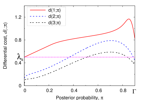
Figure 1: Differential costs, $d(\cdot;\pi)$, for $n=10$ sensors, $\lambda_{f}=100.0$, $\lambda_{s}=0.5$, $f_{0}\sim\mathcal{N}(0,1)$ and $f_{1}\sim\mathcal{N}(1,1)$.

III-B Control on the probability of a sensor in the ${\sf awake}$ state

In this subsection, we are interested in obtaining an optimal control on $q_{k+1}$, the probability of a sensor in the ${\sf awake}$ state, based on the information we have at time slot $k$, instead of determining the number of sensors that must be in the ${\sf awake}$ state in the next slot.

At time slot $k$, after having observed ${\bf X}_{k}^{{\cal M}_{k}}$, the fusion centre computes the sufficient statistic $\Pi_{k}$, based on which it makes a decision to ${\sf stop}$ or to ${\sf continue}$ sampling. If the decision is to ${\sf continue}$ at time slot $k+1$, the fusion centre (also acts as a controller) chooses $q_{k+1}$, the probability of a sensor to be in the ${\sf awake}$ state at time slot $k+1$. Thus, the set of controls at time slot $k$ is given by $\mathcal{A}~{}=~{}\bigg{\{}(\mathsf{stop},0),\cup_{q\in[0,1]}(\mathsf{continue},q)\bigg{\}}$ = $\bigg{\{}1,\cup_{q\in[0,1]}(0,q)\bigg{\}}=\{(1,0),\{0\}\times[0,1]\}$.

When the control $A_{k}=(0,q_{k+1})$ is chosen, $M_{k+1}$, the number of sensors in the ${\sf awake}$ state at time slot $k+1$ is Bernoulli distributed with parameters $(n,q_{k+1})$. Let $\gamma_{m}(q_{k+1})$ be the probability that $m$ sensors are in the ${\sf awake}$ state at time slot $k+1$. $\gamma_{m}(q_{k+1})$ is given by

$$\gamma_{m}(q_{k+1}) = \binom{n}{m}q_{k+1}^{m}(1-q_{k+1})^{n-m}.$$ (30)

The information state at time slot $k$ $\Pi_{k}$, can be computed in a recursive manner from $\Pi_{k-1}$, $A_{k-1}$ and ${\bf X}_{k}^{{\cal M}_{k}}$ using Eqn. 20. Thus, it is clear that the $\{\Pi_{k}\}$ process is a controlled Markov process, the state space of the process being $\mathcal{S}=[0,1]\cup\{{\sf t}\}$. Motivated by the cost function given in Eqn. 11, define the one stage cost function $\widetilde{c}\left(s,a\right)$ when the (state,action) pair is $(s,a)$ as

$$\widetilde{c}\left(s,a\right) = \left\{\begin{array}[]{ll}\lambda_{f}(1-\pi),&\text{if}\ s=\pi\in[0,1],a=(1,0)\\ \pi+\lambda_{s}nq,&\text{if}\ s=\pi\in[0,1],a=(0,q)\\ 0,&\text{if}\ s=\mathsf{t}.\end{array}\right.$$

Since, the one stage cost and the density function $\phi_{2}({\bf y};\widetilde{\Pi}_{k-1})$ are time invariant, it is sufficient to consider the class of stationary policies (see Proposition 2.2.2 of [13]). Let $\widetilde{\mu}:\mathcal{S}\to\mathcal{A}$ be a stationary policy. Hence, the cost of using the policy $\widetilde{\mu}$ is given by

$$J_{\widetilde{\mu}}(\pi_{0}) = \mathsf{E}\!\left[\sum_{k=0}^{\infty}\widetilde{c}(\Pi_{k},\widetilde{\mu}(\Pi_{k}))\bigg{\arrowvert}\Pi_{0}=\pi_{0}\right],$$

and hence the minimal cost among the class of stationary policies is given by

$$J^{*}(\pi_{0}) = \min_{\widetilde{\mu}}\mathsf{E}\!\left[\sum_{k=0}^{\infty}\widetilde{c}(\Pi_{k},\widetilde{\mu}(\Pi_{k}))\bigg{\arrowvert}\Pi_{0}=\pi_{0}\right].$$

The DP that solves the above problem is given by the Bellman’s equation,

$$J^{*}(\pi) = \min\left\{\widetilde{c}(\pi,1),H_{J^{*}}(\pi)\right\}$$

where $H_{J^{*}}:[0,1]\to{\mathbb{R}}_{+}$ is defined as

$$H_{J^{*}}(\pi)$$

$$:= \min_{0\leq q\leq 1}\left\{\widetilde{c}(\pi,(0,q))+\sum_{m=0}^{n}\gamma_{m}(q)\mathsf{E}_{\phi_{2}({\bf y};\tilde{\pi})}\!\left[J^{*}\big{(}\Phi(\pi,(0,m),{\bf Y}\big{)}\right]\right\}$$

where ${\bf Y}$ and ${\bf y}$ are $m$–vectors. Recall that the expectation is taken with respect to the pdf $\phi_{2}({\bf y};\tilde{\pi})$. The Bellman’s equation can be written as

$$J^{*}(\pi) = \min\left\{\lambda_{f}\cdot\big{(}1-\pi\big{)},\pi+A_{J^{*}}\big{(}\pi\big{)}\right\}$$ (32)

where the function $A_{J^{*}}:[0,1]\to\mathbb{R}_{+}$ is defined as

$$A_{J^{*}}(\pi)$$

$$= \min_{q\in[0,1]}\left\{\lambda_{s}nq+\sum_{m=0}^{n}\gamma_{m}(q)\mathsf{E}_{\phi_{2}({\bf y};\tilde{\pi})}\!\left[J^{*}\left(\frac{\tilde{\pi}\cdot\phi_{1}({\bf Y})}{\phi_{2}({\bf Y};\tilde{\pi})}\right)\right]\right\}.$$

The optimal policy $\mu^{*}$ gives the optimal stopping time $\tau^{*}$, and the optimal probabilities, $q_{k}^{*},\ k~{}=~{}1,2,\cdots,\tau^{*}$. The structure of the optimal policy is shown in the following theorems.

Theorem 5

The total cost function $J^{*}(\pi)$ is concave in $\pi$.

Theorem 6

The optimal stopping rule is a threshold rule where the threshold is on the a posteriori probability of change,

$$\tau^{*} = \inf\{k:\Pi_{k}\geqslant\Gamma\},$$

for some $\Gamma\in[0,1]$. The threshold $\Gamma$ depends on the probability of false alarm constraint, $\alpha$ (among other parameters like the distribution of $T$, $f_{0}$, $f_{1}$).

IV Quickest Change Detection without Feedback

In this section, we study the ${\sf sleep}$–${\sf wake}$ scheduling problem defined in Eqn. 16. Open loop control is applicable to the systems in which there is no feedback channel from the fusion centre (controller) to the sensors. Here, at any time slot $k$, a sensor chooses to be in the ${\sf awake}$ state with probability $q$ independent of other sensors. Hence, $\{M_{k}\}$, the number of sensors in the ${\sf awake}$ state at time slot $k$ is i.i.d. Bernoulli distributed with parameters $(n,q)$. Let $\gamma_{m}$ be the probability that $m$ sensors are in the ${\sf awake}$ state. $\gamma_{m}$ is given by

$$\gamma_{m} = \binom{n}{m}q^{m}(1-q)^{n-m}$$ (33)

We choose $q$ that minimises the Bayesian cost given by Eqn. 16.

At time slot $k$, the fusion centre receives a vector of observation ${\bf X}_{k}^{{\cal M}_{k}}$ and computes $\Pi_{k}$. In the open loop scenario, the state space is $\mathcal{S}=\big{\{}[0,1]\cup\{\mathsf{t}\}\big{\}}$. The set of actions is given by $\mathcal{A}=\{\mathsf{stop},\mathsf{continue}\}=\{1,0\}$ where ‘1’ represents ${\sf stop}$ and ‘0’ represents ${\sf continue}$. Note that $\Pi_{k}$ can be computed from $\Pi_{k-1},A_{k-1}$, and ${\bf X}_{k}^{{\cal M}_{k}}$ in the same way as shown in Eqn. 20. Thus, $\{\Pi_{k}\}$, $k\in\mathbb{Z}_{+}$ is a controlled Markov process. Motivated by the structure of the cost given in Eqn. 11, we define the one stage cost function $\widetilde{c}:\mathcal{S}\times\mathcal{A}\to\mathbb{R}_{+}$ when the (state, action) pair is $(s,a)$ as

$$\widetilde{c}(s,a) = \left\{\begin{array}[]{ll}\lambda_{f}(1-\pi),&\text{if}\ s=\pi\in[0,1],a=1\\ \pi+\lambda_{s}nq,&\text{if}\ s=\pi\in[0,1],a=0\\ 0,&\text{if}\ s=\mathsf{t}.\end{array}\right.$$

Since, the one stage cost and the density function $\phi_{2}({\bf y};\widetilde{\Pi}_{k-1})$ are time invariant, it is sufficient to consider the class of stationary policies (see Proposition 2.2.2 of [13]). Let $\widetilde{\mu}:\mathcal{S}\to\mathcal{A}$ be a stationary policy. Hence, the cost of using the policy $\widetilde{\mu}$ is given by

$$J_{\widetilde{\mu}}(\pi_{0}) = \mathsf{E}\!\left[\sum_{k=0}^{\infty}\widetilde{c}(\Pi_{k},\widetilde{\mu}(\Pi_{k}))\bigg{\arrowvert}\Pi_{0}=\pi_{0}\right],$$

and the optimal cost under the class of stationary policies is given by

$$J^{*}(\pi_{0}) = \min_{\widetilde{\mu}}\mathsf{E}\!\left[\sum_{k=0}^{\infty}\widetilde{c}(\Pi_{k},\widetilde{\mu}(\Pi_{k}))\bigg{\arrowvert}\Pi_{0}=\pi_{0}\right]$$

The DP that solves the above equation is given by the Bellman’s equation,

$$J^{*}(\pi) = \min\bigg{\{}\widetilde{c}(\pi,1),H_{J^{*}}(\pi)\bigg{\}}$$

where $H_{J^{*}}:[0,1]\to{\mathbb{R}}_{+}$ is defined as

$$H_{J^{*}}(\pi):=\widetilde{c}(\pi,0)+\sum_{m=0}^{n}\gamma_{m}\mathsf{E}_{\phi_{2}({\bf y};\tilde{\pi})}\!\left[J^{*}\bigg{(}\Phi(\pi,(0,m),{\bf Y})\bigg{)}\right]$$

where ${\bf Y}$ and ${\bf y}$ are $m$–vectors. The above equation can be written as

$$J^{*}(\pi) = \min\left\{\lambda_{f}\cdot\big{(}1-\pi\big{)},\pi+A_{J^{*}}\big{(}{\pi}\big{)}\right\}.$$ (35)

where the function $A_{J^{*}}:[0,1]\to\mathbb{R}_{+}$ is defined as

$$A_{J^{*}}({\pi})= \lambda_{s}nq+\sum_{m=0}^{n}\gamma_{m}\mathsf{E}_{\phi_{2}({\bf y};\tilde{\pi})}\!\left[J^{*}\left(\frac{\tilde{\pi}\cdot\phi_{1}({\bf Y})}{\phi_{2}({\bf Y};\tilde{\pi})}\right)\right].$$

The optimal policy $\mu^{*}$ that achieves $J^{*}$ gives the optimal stopping rule, $\tau^{*}$. We now prove some properties of the optimal policy.

Theorem 7

The optimal total cost function $J^{*}(\pi)$ is concave in $\pi$.

Theorem 8

The optimal stopping rule is a threshold rule where the threshold is on the a posteriori probability of change,

$$\tau^{*} = \inf\{k:\Pi_{k}\geqslant\Gamma\},$$

for some $\Gamma\in[0,1]$. The threshold $\Gamma$ depends on the probability of false alarm constraint, $\alpha$ (among other parameters like the distribution of $T$, $f_{0}$, $f_{1}$).

For each $q\in[0,1]$, we compute the optimal mean detection delay ${\sf E_{DD}}$ (as a function of $q$), and then find the optimal $q^{*}$ for which the optimal mean detection delay is minimum.

V Numerical Results

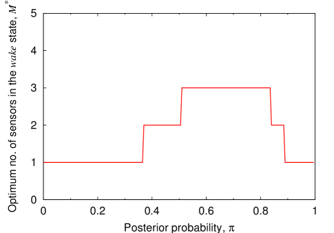
Figure 2: Optimum number of sensors in the ${\sf awake}$ state $M^{*}$ for $n=10$ sensors, $\lambda_{f}=100.0$, $\lambda_{s}=0.5$, $f_{0}\sim\mathcal{N}(0,1)$ and $f_{1}\sim\mathcal{N}(1,1)$. Note that $\Gamma=0.9$ corresponds to the threshold.

We compute the optimal policy for each of the ${\sf sleep}$–${\sf wake}$ scheduling strategies given in Eqns. 26, 32, 35 using value–iteration technique (see [12]). We consider $n=10$ sensors. The distributions of change–time $T$ is taken to be geometric $(0.01)$ (and $\pi_{0}=0$). Also, the prechange and the postchange distributions of the sensor observations are taken to be $\mathcal{N}(0,1)$ and $\mathcal{N}(1,1)$. We set the cost per observation per sensor, $\lambda_{s}$ to 0.5 and the cost of false alarm, $\lambda_{f}$ to 100.0 (this corresponds to $\alpha=$ 0.04).

• Optimal control of $M_{k+1}$:

  We compute $M^{*}$ the optimal number of sensors to be in the ${\sf awake}$ state in time slot $k+1$ as a function of the a posteriori probability of change $\pi$ (from the optimal policy $\mu^{*}$ given by Eqn.26) by the value iteration algorithm [13], [14] and plot in Figure 2. We note that in any time slot, it is not economical to use more than 3 sensors (though we have 10 sensors). Also, from Figure 2, it is clear that $M^{*}$ increases monotonically for $\pi<0.6$ and then decreases monotonically for $\pi\geq 0.6$. Note that, the region $\pi\in[0.5,\ 0.82]$ requires many sensors for optimal detection whereas the region $[0.0,\ 0.3]\cup[0.9,\ 1.0]$ requires the least number of sensors. This is due to the fact that uncertainty is more in the region $\pi\in[0.5,\ 0.82]$ whereas it is less in the region $[0.0,\ 0.3]\cup[0.9,\ 1.0]$.

  In Figure 3, we plot the trajectory of a sample path of $\Pi_{k}$ versus the time slot $k$. In our numerical experiment, the event occurs at $T=152$. When the number of sensors to be in the ${\sf awake}$ state $M_{k+1}$ is $M^{*}(\pi_{k})$ (taken from Figure 2), for a threshold of 0.9, we see that the detection happens at $\tau_{M^{*}}=161$. When $M_{k+1}=10$ sensors (no ${\sf sleep}$ scheduling), we find the detection epoch to be $\tau_{10}=153$. When $M_{k+1}=3$ sensors (we chose 3 because $M^{*}\leq 3$), the stopping happens at $\tau_{3}=156$. From the above stopping times, it is clear that the detection delay does not vary significantly in the above three cases. By having an optimal ${\sf sleep}$–$\sf wake$ scheduling, we observe that until the event occurs only one sensor is in ${\sf awake}$ state and as soon as the event occurs, the ${\sf sleep}$–$\sf wake$ scheduler ramps up the number of sensors to 3, thereby making a quick decision. Thus, the optimal ${\sf sleep}$–$\sf wake$ scheduling uses a minimal number of sensors before change and quickly ramps up the number of sensors after change for quick detection. Also, we see from Figure 3, that the $\pi_{k}$ trajectory corresponding to $M_{k+1}(\pi)=10$ (and $M_{k+1}(\pi)=3$) gives more reliable information about the event than the $\pi_{k}$ trajectory corresponding to $M_{k+1}(\pi)=M^{*}$.

  

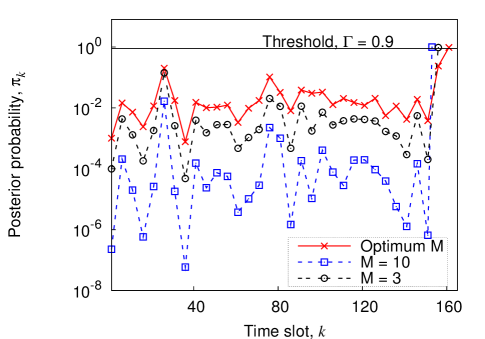
  Figure 3: A sample run of event detection with $n=10$ sensors, $\lambda_{f}=100.0$, $\lambda_{s}=0.5$, $f_{0}\sim\mathcal{N}(0,1)$ and $f_{1}\sim\mathcal{N}(1,1)$.

  

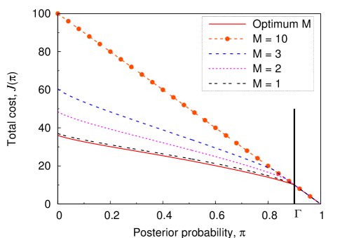
  Figure 4: Total cost $J(\pi)$ for $n=10$ sensors, $\lambda_{f}=100.0$, $\lambda_{s}=0.5$, $f_{0}\sim\mathcal{N}(0,1)$ and $f_{1}\sim\mathcal{N}(1,1)$. Note that the threshold corresponding to $M=1$ is 0.895, for $M=2$ is 0.870, for $M=3$ is 0.825, and for $M^{*}$ is $\Gamma=0.9$.

  

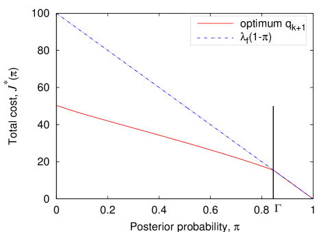
  Figure 5: Total cost $J^{*}(\pi)$ for $n=10$ sensors, $\lambda_{f}=100.0$, $\lambda_{s}=0.5$, $f_{0}\sim\mathcal{N}(0,1)$ and $f_{1}\sim\mathcal{N}(1,1)$. The dashed line $\lambda_{f}(1-\pi)$ is the cost of false alarm.

  We also plot the total cost function $J(\pi)$ for the above cases in Figure 4. Though the detection delays do not vary much, the total cost varies significantly. This is because the event happens at time slot $T=152$. In the case of $M_{k+1}=M^{*}$, it is clear from Figures 2 and 3 that only one sensor is used for the first 158 time slots. This reduces the cost by 10 times compared to the case of $M_{k+1}=10$ (in this sample path) and about 3 times compared to the case of $M_{k+1}=3$ (in this sample path). We note from Figure 4, that it is better to keep 3 sensors active all the time than keeping 10 sensors active all the time. Also, in the case of $M_{k+1}=1$, after the event occurs, the a posteriori probability takes more time to cross the threshold compared to the optimal ${\sf sleep}$–$\sf wake$ (which quickly ramps up from 1 to 3 sensors) and hence, the total cost corresponding to $M_{k+1}=1$ is slightly worse than that of $M_{k+1}=M^{*}$.

• Optimal control of $q_{k+1}$: In the case of control on $q_{k}$, we consider the same set of parameters as in the case of control on $M_{k}$. We computed the optimal policy from the DP defined in Eqn. 32 by value iteration. The optimal policy also gives the optimal probability of choosing a sensor in the ${\sf awake}$ state, $q^{*}_{k+1}$. We plot the total cost $J^{*}(\pi)$ in Figure 5. We also plot the optimum probability of a sensor in the ${\sf awake}$ state, $q^{*}(\pi)$ in Figure 6. We observe that for $\pi\leq 0.72$, $q^{*}(\pi)$ is an increasing function of $\pi$, and for $\pi>0.72$, $q^{*}(\pi)$ decreases with $\pi$. This agrees well with the intuition for the optimal control on $M_{k+1}$.

  

  Figure 6: Optimum probability of a sensor in the ${\sf awake}$ state, $q_{k+1}^{*}(\pi)$ for $n=10$ sensors, $\lambda_{f}=100.0$, $\lambda_{s}=0.5$, $f_{0}\sim\mathcal{N}(0,1)$ and $f_{1}\sim\mathcal{N}(1,1)$.

  

  Figure 7: Total cost $J^{*}(0)$ for $n=10$ sensors, $\lambda_{f}=100.0$, $f_{0}\sim\mathcal{N}(0,1)$ and $f_{1}\sim\mathcal{N}(1,1)$.

• Open loop control on $q$:

  We consider the same set of parameters for the case of open loop control on $q$. We obtain $J^{*}(0)$ for various values of $q$ and plotted in the Figure 7. We obtain the plot for $\lambda_{s}=0.5$ and for $\lambda_{s}=0.0$. In the special case of $q=1$, i.e., having $M_{k+1}=10$ sensors, and with $\lambda_{s}=0.5$, we observe that the total cost is 100 which matches with the corresponding cost in Figure 4. Also, in the limiting case of $q\to 0$, all the sensor nodes are in the ${\sf sleep}$ state at all time slots, and the detection happens only based on Bayesian update (i.e., based on the prior distribution of $T$). Thus at $q=0$, the total cost is the same (which is 73) for $\lambda_{s}=0.5$ and $\lambda_{s}=0.0$ which is also evident from Figure 7.

  Note that when $\lambda_{s}>0$, for low values of $q$, the detection delay cost dominates over the observation costs in $J^{*}(0)$ and for high values of $q$, the observation costs dominate over the detection delay cost. Thus, there is a trade–off between the detection delay cost and the observation costs as $q$ varies. This is captured in the Figure 7. Note that the Bayesian cost is optimal at $q=0.15$. When $\lambda_{s}=0$, as $q$ increases the detection delay decreases. Hence, we see the monotonically decreasing trend for $\lambda_{s}=0.0$.

From Figures 4, 5, and 7, we note that the total cost $J(\pi)$ is the least for optimal control on $M_{k+1}$. Also, we note that in the open loop control case, the least total cost $J^{*}(0)=55$ is achieved when the attempt probability, $q$ is $0.15$ (see Figure 7; this corresponds to an average of 1.5 sensors being active). It is to be noted that this cost is larger than that achieved by the optimal closed loop policies ($J^{*}(0)=50$ for the closed loop control on $q_{k+1}$ and $J^{*}(0)=38$ for the closed loop control on $M_{k+1}$). From Figures 3 and 2, we see that when $M_{k+1}(\pi)=M^{*}(\pi)$, the switching of the sensors between ${\sf sleep}$ and ${\sf awake}$ states happen only in 2 slots out of 161 slots. Otherwise only 1 sensor is on.

VI Conclusion

In this paper, we formulated the problem of jointly optimal ${\sf sleep}$–${\sf wake}$ scheduling and event detection in a sensor network that minimises the detection delay and the usage of sensing/communication resources. We have set out to solve the problem in Eqn. 13. We have derived the optimal control for three approaches using the theory of MDP. We showed the existence of the optimal policy and obtained some structural results.

We prescribe the ${\sf sleep}$–${\sf wake}$ scheduling policies as follows: When there is a feedback between the fusion centre and the sensors and if the feedback is unicast, it is optimal to use the control on $M_{k+1}$ policy; when the feedback is only broadcast, then it is optimal to use the control on $q_{k+1}$. If there is no feedback between the fusion centre and the sensors, we prescribe the open loop control on $q$ policy.

Proof of Theorem 1

We use the following Lemma to prove Theorem 1.

Lemma 1

If $f:[0,1]\to\mathbb{R}$ is concave, then for any ${\bf x}\in{\mathbb{R}}^{m}$ (for any $m\in\mathbb{Z}_{+}$), the function $h:[0,1]\to\mathbb{R}$ defined by

$$h(y) ={\mathsf{E}}_{\phi_{2}({\bf x};y)}\left[f\left(\frac{y\phi_{1}({\bf X})}{y\phi_{1}({\bf X})+(1-y)\phi_{0}({\bf X})}\right)\right]$$

is concave in $y$, where $\phi_{1}({\bf x})$ and $\phi_{0}({\bf x})$ are pdfs on ${\bf X}$, and $\phi_{2}({\bf x};y)=y\phi_{1}({\bf x})+(1-y)\phi_{0}({\bf x})$.

Proof For any given ${\bf x}$, define the function $h_{1}:[0,1]\to\mathbb{R}$ as

$$h_{1}(y;{\bf x})$$

$$:= f\left(\frac{y\phi_{1}({\bf x})}{y\phi_{1}({\bf x})+(1-y)\phi_{0}({\bf x})}\right)\Big{[}y\phi_{1}({\bf x})+(1-y)\phi_{0}({\bf x})\Big{]}.$$

As ${\mathsf{T}}:=\int\cdots\ d{\bf x}$ is a linear operator and $h(y)=\mathsf{T}h_{1}(y;{\bf x})$, it is sufficient to show that $h_{1}(y;{\bf x})$ is concave in $y$. If $f(y)$ is concave then (see [15])

$$f(y) =\inf_{(a_{i},b_{i})\in I}\big{\{}a_{i}y+b_{i}\big{\}}$$

where $I=\{(a,b)\in\mathbb{R}^{2}:ay+b\geq f(y),y\in[0,1]\}$. Hence,

$$h_{1}(y;{\bf x})$$

$$= f\left(\frac{y\phi_{1}({\bf x})}{y\phi_{1}({\bf x})+(1-y)\phi_{0}({\bf x})}\right)\Big{[}y\phi_{1}({\bf x})+(1-y)\phi_{0}({\bf x})\Big{]}$$

$$= \inf_{(a_{i},b_{i})\in I}\left\{a_{i}\left(\frac{y\phi_{1}({\bf x})}{y\phi_{1}({\bf x})+(1-y)\phi_{0}({\bf x})}\right)+b_{i}\right\}$$

$$\cdot\Big{[}y\phi_{1}({\bf x})+(1-y)\phi_{0}({\bf x})\Big{]}$$

$$= \inf_{(a_{i},b_{i})\in I}\left\{a_{i}y\phi_{1}({\bf x})+b_{i}\Big{[}y\phi_{1}({\bf x})+(1-y)\phi_{0}({\bf x})\Big{]}\right\}$$

$$= \inf_{(a_{i},b_{i})\in I}\left\{\Big{(}(a_{i}+b_{i})\phi_{1}({\bf x})-b_{i}\phi_{0}({\bf x})\Big{)}y+b_{i}\phi_{0}({\bf x})\right\}$$

which is an infimum of a collection of affine functions of $y$. This implies that $h_{1}(y;{\bf x})$ is concave in $y$ (see [15]). $\hfill\blacksquare$

The optimal total cost function $J^{*}(\pi)$ can be computed using a value iteration algortithm. Here, we first consider a finite $K$–horizon problem and then we let $k\to\infty$, to obtain the infinite horizon problem.

Note that the cost–to–go function, $J_{K}^{K}(\pi)=\lambda_{f}\cdot\big{(}1-\pi\big{)}$ is concave in $\pi$. Hence, by Lemma 1, we see that the cost–to–go functions $J_{K-1}^{K}(\pi),$ $J_{K-2}^{K}(\pi),$ $\cdots,J_{0}^{K}(\pi)$ are concave in $\pi$. Hence for $0\leq\lambda\leq 1$,

$$J^{*}(\pi) =\lim_{K\rightarrow\infty}J^{K}_{0}(\pi)$$

$$J^{*}(\lambda\pi_{1}+(1-\lambda)\pi_{2}) =\lim_{K\rightarrow\infty}J^{K}_{0}\Big{(}\lambda\pi_{1}+(1-\lambda)\pi_{2}\Big{)}$$

$$\geq\lim_{K\rightarrow\infty}\lambda J^{K}_{0}(\pi_{1})+\lim_{K\rightarrow\infty}(1-\lambda)J^{K}_{0}(\pi_{2})$$

$$=\lambda J^{*}(\pi_{1})+(1-\lambda)J^{*}(\pi_{2})$$

It follows that $J^{*}(\pi)$ is concave in $\pi$. $\hfill\blacksquare$

Proof of Theorem 2

Define the maps $C:[0,1]\to\mathbb{R}_{+}$ and $H:[0,1]\to\mathbb{R}_{+}$, as

$$C(\pi) :=\lambda_{f}\cdot\big{(}1-\pi\big{)}$$

$$H(\pi) :=\pi+A_{J^{*}}(\pi)$$

Note that $C(1)=0$, $H(1)=1$, $C(0)=\lambda_{f}$ and $H(0)=A_{J^{*}}(0)$. Note that

$$A_{J^{*}}(0)$$

$$= \min_{0\leq m\leq n}\left\{\lambda_{s}m+{\mathsf{E}}_{\phi_{2}({\bf X}^{({m})};p)}\left[J^{*}\left(\frac{{p}\cdot\phi_{1}({\bf X}^{(m)})}{\phi_{2}({\bf X}^{(m)};p)}\right)\right]\right\}$$

$$\leq \min_{0\leq m\leq n}\left\{\lambda_{s}m+J^{*}\left({\mathsf{E}}_{\phi_{2}({\bf X}^{({m})};p)}\left[\frac{p\cdot\phi_{1}({\bf X}^{(m)})}{\phi_{2}({\bf X}^{(m)};p)}\right]\right)\right\}$$

$$= \min_{0\leq m\leq n}\left\{\lambda_{s}m+J^{*}\left(p\right)\right\}$$

$$= J^{*}\left(p\right)$$

$$\leq \lambda_{f}\cdot\big{(}1-p\big{)}\ \ \ \text{(from Eqn.~{}16)}$$

The inequality in the second step is justified using Jensen’s inequality and the inequality in the last step follows from the definition of $J^{*}$.

Note that $H(1)-C(1)>0$ and $H(0)-C(0)<0$. As the function $H(\pi)-C(\pi)$ is concave, by the intermediate value theorem, there exists $\Gamma\in[0,1]$ such that $H(\Gamma)=C(\Gamma)$. This $\Gamma$ is unique as $H(\pi)=C(\pi)$ for at most two values of $\pi$. If in the interval $[0,1]$, there are two distinct values of $\pi$ for which $H(\pi)=C(\pi)$, then the signs of $H(0)-C(0)$ and $H(1)-C(1)$ should be the same. Hence, the optimal stopping rule is given by

$$\tau^{*} =\inf\left\{k:\Pi_{k}\geq\Gamma\right\}$$

where the threshold $\Gamma$ is given by $\Gamma+A_{J^{*}}(\Gamma)=\lambda_{f}\cdot\big{(}1-\Gamma\big{)}$.

$\hfill\blacksquare$

Proof of Theorem 3

Define

$$\phi_{j}({\bf x}^{(m)}) := \prod_{i=1}^{m}f_{j}(x^{(i)}),\ j=0,1.$$

$${\bf x}^{(l)} := (x^{(1)},x^{(2)},\cdots,x^{(m)},x^{(m+1)},\cdots,x^{(l)})$$

$${\bf u} := (x^{(1)},x^{(2)},\cdots,x^{(m)})$$

$${\bf v} := (x^{(m+1)},x^{(m+2)},\cdots,x^{(l)})$$

$$\hat{\pi} := \frac{\tilde{\pi}\phi_{1}({\bf u})}{\tilde{\pi}\phi_{1}({\bf u})+(1-\tilde{\pi})\phi_{0}({\bf u})}$$

Note that

$$B_{J^{*}}^{(l)}({\pi})$$

$$= \int_{{\mathbb{R}^{l}}}J^{*}\left(\frac{{\tilde{\pi}}\cdot\phi_{1}({\bf x}^{(l)})}{\phi_{2}({\bf x}^{(l)};\tilde{\pi})}\right)\Big{[}\phi_{2}({\bf x}^{({l})};\tilde{\pi})\Big{]}\ d{\bf x}^{(l)}$$

$$= \int_{{\mathbb{R}^{m}}}\int_{\mathbb{R}^{l-m}}J^{*}\left(\frac{\hat{\pi}\phi_{1}({\bf v})}{\phi_{2}({\bf{v}};\hat{\pi})}\right)\phi_{2}({\bf{v}};\hat{\pi})\ d{\bf v}\phi_{2}({\bf{u}};\tilde{\pi})\ d{\bf u}$$

$$\leq \int_{{\mathbb{R}^{m}}}J^{*}\left(\int_{\mathbb{R}^{l-m}}\frac{\hat{\pi}\phi_{1}({\bf v})}{\phi_{2}({\bf{v}};\hat{\pi})}\Big{[}\phi_{2}({\bf{v}};\hat{\pi})\Big{]}d{\bf v}\right)\phi_{2}({\bf{u}};\tilde{\pi})\ d{\bf u}$$

$$= \int_{{\mathbb{R}^{m}}}J^{*}\left(\hat{\pi}\right)\phi_{2}({\bf{u}};\tilde{\pi})d{\bf u}$$

$$= B_{J^{*}}^{(m)}({\pi})$$

As $J^{*}$ is concave, the inequality in the second line follows from Jensen’s inequality. Hence proved. $\hfill\blacksquare$

Proof of Theorem 4

Eqn. 27 and the monotone property of $d(m;.)$ proves the theorem. $\hfill\blacksquare$

Proof of Theorem 5

Follows from the proof of Theorem 1. $\hfill\blacksquare$

Proof of Theorem 6

Follows from the proof of Theorem 2. $\hfill\blacksquare$

Proof of Theorem 7

Follows from the proof of Theorem 1. $\hfill\blacksquare$

Proof of Theorem 8

Follows from the proof of Theorem 2. $\hfill\blacksquare$

References

- [1] A. N. Shiryaev, “On optimum methods in quickest detection problems,” Theory of Probability and its Applications, vol. 8, no. 1, pp. 22–46, 1963.
- [2] C. Rago, P. Willet, and Y. Bar-Shalom, “Censoring sensors: A low communication-rate scheme for distributed detection,” IEEE Transactions on Aerospace and Electronic Systems, vol. 32, no. 2, pp. 554–568, April 1996.
- [3] S. Appadwedula, V. V. Veeravalli, and D. L. Jones, “Energy-efficient detection in sensor networks,” IEEE J. Sel. Areas Commun., vol. 23, no. 4, pp. 693–702, April 2005.
- [4] Y. Wu, S. Fahmy, and N. B. Shroff, “Energy efficient sleep/wake scheduling for multi-hop sensor networks: Non-convexity and approximation algorithm,” in Infocom, Alaska, USA, May 2007.
- [5] L. Zacharias and R. Sundaresan, “Decentralized sequential change detection using physical layer fusion,” in IEEE ISIT, Nice, France, Jun. 2007.
- [6] R. Solis, V. S. Borkar, and P. R. Kumar, “A new distributed time synchronization protocol for multihop wireless networks,” in 45th IEEE Conference on Decision and Control (CDC’06), December 2006.
- [7] A. N. Shiryaev, Optimal Stopping Rules. New York: Springer, 1978.
- [8] V. V. Veeravalli, “Decentralized quickest change detection,” IEEE Transactions on Information theory, vol. 47, no. 4, pp. 1657–1665, May 2001.
- [9] V. K. Prasanthi and A. Kumar, “Optimizing delay in sequential change detection on ad hoc wireless sensor networks,” in IEEE SECON, VA, USA, Sep. 2006.
- [10] K. Premkumar, V. K. Prasanthi, and A. Kumar, “Delay optimal event detection on ad hoc wireless sensor networks,” ACM Transactions on Sensor Networks, to appear.
- [11] E. L. Lehmann and G. Casella, Theory of Point Estimation. New York: Springer–Verlag, 1998.
- [12] D. P. Bertsekas, Dynamic Programming and Optimal Control, 2nd ed. Athena Scientific, 2000, vol. I.
- [13] ——, Dynamic Programming and Optimal Control, 3rd ed. Athena Scientific, 2007, vol. II.
- [14] O. Hernández-Lerma and J. B. Lasserre, Discrete–Time Markov Control Processes:Basic Optimality Criteria. New York: Springer–Verlag, 1996.
- [15] R. T. Rockafellar, Convex Analysis. Princeton, New Jersy: Princeton University Press, 1997.