Canonical Quantization for a Relativistic Neutral Scalar Field
in Non-equilibrium Thermo Field Dynamics

Abstract

A relativistic neutral scalar field is investigated in non-equilibrium thermo field dynamics. The canonical quantization is applied to the fields out of equilibrium. Because the thermal Bogoliubov transformation becomes time-dependent, the equations of motion for the ordinary unperturbed creation and annihilation operators are modified. This forces us to introduce a thermal counter term in the interaction Hamiltonian which generates additional radiative corrections. Imposing the self-consistency renormalization condition on the total radiative corrections, we obtain the quantum Boltzmann equation for the relativistic scalar field.

1 Introduction

A scattering process is described by a relativistic quantum field theory at high energy. The quantum field theory has to be extended to study an out of equilibrium system for a relativistic field. There are several formalisms to introduce a thermal property in the quantum field theory, for example, thermo field dynamics, closed time path formalism and Langevin equation[1, 2, 3]. The thermo field dynamics (TFD) is a real time formalism based on the canonical quantization.[4, 5, 7, 6] In TFD the thermal Bogoliubov transformation is introduced with particle number density and the thermal Bogoliubov transformed oscillator defines the so-called thermal vacuum state. The thermal average of a dynamical operator is represented as an expectation value in the thermal vacuum state.

Much attention has been paid to generalize it for an out of equilibrium system and derive the time evolution equation for a particle number distribution. The non-equilibrium thermo field dynamics (NETFD) is constructed by extending the thermal Bogoliubov transformation in Ref. netfd1. The Boltzmann-like equation for a non-relativistic particle is found by the time evolution equation for the expectation value of the particle number operator with perturbed oscillators in Ref. matsumoto3.

In NETFD the thermal counter term is introduced from the consistency of the time evolution for an ordinary oscillator and the thermal Bogoliubov transformed one [10, 11, 12]. The Boltzmann equation is derived from the self-consistency renormalization condition which is imposed on the quantum corrections with the thermal counter term.[13, 14] The method was extended to an inhomogeneous system with diffusion.[15, 16] Recently NETFD is applied to evaluate the Bose-Einstein condensation in trapped cold atom systems.[17, 18, 19, 20]

NETFD for a relativistic field is necessary to study the thermalization process of quarks and gluons in ultrarelativistic heavy ion collisions. An out of equilibrium system for a relativistic field is also essential in critical phenomena at early universe. Several works have been done for a relativistic field in NETFD[21, 22]. However, the canonical formalism of NETFD has not been fully established for a relativistic field yet. Thus we have launched our plan to make a systematic study of the canonical quantization in NETFD based on the thermal Bogoliubov transformation.

In this paper we focus on a relativistic neutral scalar field and investigate the canonical quantization in a homogeneous system. In §2 we briefly review TFD for a scalar field. The thermal Bogoliubov transformation is made time-dependent for an out of equilibrium system in NETFD, in accordance with time-dependent particle number distribution. In §3 we discuss how to decompose the neutral scalar field. In §4 the scalar field is quantized in the canonical formalism. We introduce the thermal counter term and calculate the scalar propagator. The self-consistency condition is introduced from the structure of the scalar propagator. The time evolution equation is obtained from the self-consistency renormalization condition. In §5 it is confirmed that the self-consistency condition implies the correspondence between the thermal Bogoliubov parameter and the particle number density, given by an expectation of the Heisenberg number density operator. We impose the condition on the neutral scalar field with self-interactions. Concluding remarks are given in §6.

2 Non-equilibrium thermo field dynamics

There are several real time formalisms to introduce thermal dynamics in a quantum field theory. TFD is one of the real time formalisms based on the canonical quantization. In TFD the statistical average of an observable quantity is represented as an expectation value of the observable operator under a pure state called thermal vacuum. The ordinary oscillator operators, after each degree of freedom is doubled as below, are related to new oscillator ones through a Bogoliubov transformation whose annihilation operator annihilates the thermal vacuum. The thermal Bogoliubov transformation is made time-dependent to deal with a non-equilibrium state in NETFD. In this section we briefly review the framework of NETFD.

In TFD the thermal degree of freedom is introduced by doubling the Fock space which is spanned by ordinary annihilation, creation operators, $(a\ \ a^{\dagger})$, and tilde ones, $(\tilde{a}\ \ \tilde{a}^{\dagger})$. For a bosonic field the operators satisfy the commutation relations,

$$[a_{p},a_{k}^{\dagger}]=(2\pi)^{3}\delta^{(3)}(\mbox{\boldmath$p$}-\mbox{\boldmath$k$}),$$ (1)

$$[\tilde{a}_{p},\tilde{a}_{k}^{\dagger}]=(2\pi)^{3}\delta^{(3)}(\mbox{\boldmath$p$}-\mbox{\boldmath$k$}),$$ (2)

$$[a_{p},\tilde{a}_{k}^{\dagger}]=0,\ \ [a_{p},\tilde{a}_{k}]=0.$$ (3)

We define the tilde conjugation rules by

$$(A_{1}A_{2})^{\sim}=\tilde{A_{1}}\tilde{A_{2}},$$ (4)

$$(c_{1}A_{1}+c_{2}A_{2})^{\sim}=c_{1}^{\ast}\tilde{A}_{1}+c_{2}^{\ast}\tilde{A}_{2},$$ (5)

$$(\tilde{A})^{\sim}=A,$$ (6)

where $A_{1}$ and $A_{2}$ mean any operators, and $c_{1}$ and $c_{2}$ are c-numbers.

Time evolution for the tilde operator is generated by the tilde conjugate of a usual Hamiltonian. The tilde-Hamiltonian, $\tilde{H}$, is constructed only from the tilde-operators. The time evolution of whole a physical system is described by a hat-Hamiltonian,

$$\hat{H}\equiv H-\tilde{H}.$$ (7)

To develop the canonical quantization in NETFD it is more convenient to rewrite the annihilation and creation operators by the transformation called the time-dependent thermal Bogoliubov transformation,

$$\xi_{p}^{\alpha}(t)=B(n_{p}(t))^{\alpha\beta}a_{p}^{\beta}(t),$$ (8)

$$\bar{\xi}_{p}^{\alpha}(t)=\bar{a}_{p}^{\beta}(t)B^{-1}(n_{p}(t))^{\beta\alpha},$$ (9)

where the upper indices, $\alpha$ and $\beta$, represent the thermal doublets,

$$a_{p}^{\alpha}=\left(\begin{array}[]{c}a_{p}\\ \tilde{a}_{p}^{\dagger}\end{array}\right),\ \ \ \bar{a}_{p}^{\alpha}=\left(\begin{array}[]{cc}a_{p}^{\dagger}&-\tilde{a}_{p}\end{array}\right),$$ (13)

$$\xi_{p}^{\alpha}=\left(\begin{array}[]{c}\xi_{p}\\ \tilde{\xi}_{p}^{\dagger}\end{array}\right),\ \ \ \bar{\xi}_{p}^{\alpha}=\left(\begin{array}[]{cc}\xi_{p}^{\dagger}&-\tilde{\xi}_{p}\end{array}\right).$$ (17)

The thermal Bogoliubov matrices, $B$ and $B^{-1}$, are chosen as

$$B(n_{p}(t))=\left(\begin{array}[]{cc}1+n_{p}(t)&-n_{p}(t)\\ -1&1\\ \end{array}\right),$$ (20)

$$B^{-1}(n_{p}(t))=\left(\begin{array}[]{cc}1&n_{p}(t)\\ 1&1+n_{p}(t)\\ \end{array}\right),$$ (23)

so that the Dyson-Wick formalism can be used.[23] Since we work in the interaction picture, the operators, $\xi_{p}(t)$ and $a_{p}(t)$, depend on time. In a particular case of equilibrium, the Bogoliubov parameter $n_{p}$ is time-independent and is taken to be the Bose-Einstein distribution. The time dependence of the transformed oscillators is given by

$$\xi_{p}^{\alpha}(t_{x})=\xi_{p}^{\alpha}e^{-i\omega_{p}t_{x}},$$ (24)

$$\bar{\xi}_{p}^{\alpha}(t_{x})=\bar{\xi}_{p}^{\alpha}e^{i\omega_{p}t_{x}},$$ (25)

where $\omega_{p}$ describes the on-shell energy for the scalar field, $\omega_{p}=\sqrt[]{\mbox{\boldmath$p$}^{2}+m^{2}}$. Though the energy, $\omega_{p}$, is not always time-independent, we confine ourselves to a system with a time-independent $\omega_{p}$, for simplicity. It should be noted that non-trivial time dependence is induced for the oscillators, $a_{p}$ and $\bar{a}_{p}$, through the time-dependent Bogoliubov parameter with momentum index, $n_{p}(t)$. For a homogeneous and isotropic system which we assume in our practical calculations below, $n_{p}(t)$ is a function of the time and the magnitude of the momentum. As will be seen in §5, the correspondence between $n_{p}(t)$ and the particle number density, given by an expectation of the Heisenberg number density operator, is shown by imposing the self-consistency renormalization condition for a non-relativistic system [4, 13, 14].

The thermal vacuum is defined by

$$\xi_{p}|\theta\rangle=\tilde{\xi}_{p}|\theta\rangle=0,$$ (26)

$$\langle\theta|\xi_{p}^{\dagger}=\langle\theta|\tilde{\xi}_{p}^{\dagger}=0.$$ (27)

The thermal vacuum state is invariant under the tilde conjugation, $(|\theta\rangle)^{\sim}=|\theta\rangle$, and $(\langle\theta|)^{\sim}=\langle\theta|$. After we perform the thermal Bogoliubov transformations (8) and (9) on the oscillators, $\xi$ and $\tilde{\xi}$, Eqs. (26) and (27) are rewritten as

$$(1+n_{p}(t))a_{p}(t)|\theta\rangle=n_{p}(t)\tilde{a}_{p}^{\dagger}(t)|\theta\rangle,$$ (28)

$$n_{p}(t)a_{p}^{\dagger}(t)|\theta\rangle=(1+n_{p}(t))\tilde{a}_{p}(t)|\theta\rangle,$$ (29)

$$\langle\theta|a_{p}(t)=\langle\theta|\tilde{a}_{p}^{\dagger}(t),$$ (30)

$$\langle\theta|a_{p}^{\dagger}(t)=\langle\theta|\tilde{a}_{p}(t).$$ (31)

Note that the thermal bra and ket vacua are not symmetric due to the choice of the thermal Bogoliubov matrices in Eqs. (20) and (23). From Eqs. (30) and (31) we can show that the interaction hat-Hamiltonian, $\hat{H}_{int}$, satisfies the following condition [4],

$$\langle\theta|\hat{H}_{int}=0,$$ (32)

(but $\hat{H}_{int}|\theta\rangle\neq 0$), which enables us to use the Dyson-Wick formalism. As is known, the Bogoliubov transformation keeps the commutation relations. Thus the transformed operators, $\xi$ and $\tilde{\xi}$, satisfy the commutation relations.

$$[\xi_{p},\xi_{k}^{\dagger}]=(2\pi)^{3}\delta^{(3)}(\mbox{\boldmath$p$}-\mbox{\boldmath$k$}),$$ (33)

$$[\tilde{\xi}_{p},\tilde{\xi}_{k}^{\dagger}]=(2\pi)^{3}\delta^{(3)}(\mbox{\boldmath$p$}-\mbox{\boldmath$k$}),$$ (34)

$$[\xi_{p},\tilde{\xi}_{k}^{\dagger}]=0,\ \ [\xi_{p},\tilde{\xi}_{k}]=0.$$ (35)

A scalar field is quantized under these commutation relations. It should be noticed that physical observables are constructed by the original operators, $a$ and $a^{\dagger}$. We would like to evaluate the expectation value for such operators under the thermal vacuum, $|\theta\rangle$.

3 Relativistic neutral scalar field in NETFD

In the previous section we have introduced the bosonic operators, $a_{p}$ and $\xi_{p}$. A scalar field can be represented by either of these operators. Since the thermal Bogoliubov transformation does not depend on the time variable in equilibrium, the time dependence of both the operators is described by the same Hamiltonian in the interaction picture. On the other hand, the time-dependent Bogoliubov transformation induces a discrepancy between the time evolution for $a_{p}$ and $\xi_{p}$ in NETFD. We introduce a decomposition of the scalar field in terms of the operator $a_{p}$ in a consistent manner.

A neutral scalar field can be represented by the operators, $\xi_{p}$ and $\bar{\xi}_{p}$, in the interaction picture,

$$\phi_{\xi}^{\alpha}(x)\equiv\int\frac{d^{3}\mbox{\boldmath$p$}}{(2\pi)^{3}}\frac{1}{\sqrt{2\omega_{p}}}(\xi_{p}^{\alpha}(t_{x})e^{i\mbox{\boldmath$p$}\cdot\mbox{\boldmath$x$}}+(\tau_{3}\bar{\xi}_{p}(t_{x})^{T})^{\alpha}e^{-i\mbox{\boldmath$p$}\cdot\mbox{\boldmath$x$}}),$$ (36)

$$\bar{\phi}_{\xi}^{\alpha}(x)\equiv\int\frac{d^{3}\mbox{\boldmath$p$}}{(2\pi)^{3}}\frac{1}{\sqrt{2\omega_{p}}}(\bar{\xi}_{p}^{\alpha}(t_{x})e^{-i\mbox{\boldmath$p$}\cdot\mbox{\boldmath$x$}}+(\xi_{p}(t_{x})^{T}\tau_{3})^{\alpha}e^{i\mbox{\boldmath$p$}\cdot\mbox{\boldmath$x$}}),$$ (37)

where $\tau_{3}$ is the third Pauli matrix acting on thermal indices. The canonical conjugates for the fields, $\phi_{\xi}$ and $\bar{\phi}_{\xi}$, are given by

$$\pi_{\xi}^{\alpha}(x)\equiv(-i)\int\frac{d^{3}\mbox{\boldmath$p$}}{(2\pi)^{3}}\sqrt{\frac{\omega_{p}}{2}}(\xi_{p}^{\alpha}(t_{x})e^{i\mbox{\boldmath$p$}\cdot\mbox{\boldmath$x$}}-(\tau_{3}\bar{\xi}_{p}(t_{x})^{T})^{\alpha}e^{-i\mbox{\boldmath$p$}\cdot\mbox{\boldmath$x$}}),$$ (38)

$$\bar{\pi}_{\xi}^{\alpha}(x)\equiv(-i)\int\frac{d^{3}\mbox{\boldmath$p$}}{(2\pi)^{3}}\sqrt{\frac{\omega_{p}}{2}}(-\bar{\xi}_{p}^{\alpha}(t_{x})e^{-i\mbox{\boldmath$p$}\cdot\mbox{\boldmath$x$}}+(\xi_{p}(t_{x})^{T}\tau_{3})^{\alpha}e^{i\mbox{\boldmath$p$}\cdot\mbox{\boldmath$x$}}).$$ (39)

These fields satisfy the canonical commutation relations at the equal time,

$$[\phi_{\xi}^{\alpha}(t,\mbox{\boldmath$x$}),\pi_{\xi}^{\beta}(t,\mbox{\boldmath$y$})]=i\delta^{(3)}(\mbox{\boldmath$x$}-\mbox{\boldmath$y$})\tau_{3}^{\alpha\beta},$$ (40)

$$[\bar{\phi}_{\xi}^{\alpha}(t,\mbox{\boldmath$x$}),\pi_{\xi}^{\beta}(t,\mbox{\boldmath$y$})]=i\delta^{(3)}(\mbox{\boldmath$x$}-\mbox{\boldmath$y$})\delta^{\alpha\beta}.$$ (41)

It is straightforward to quantize the scalar fields, $\phi_{\xi}$ and $\bar{\phi}_{\xi}$, under the thermal vacuum in a canonical formalism. However, a canonical formalism is necessary for a scalar field written by the operators $a$ and $\bar{a}$ in order to evaluate physical observables.

The time dependence of the operators, $a_{p}$ and $\bar{a}_{p}$, can be fixed by the time evolution equations for the operators, $\xi_{p}$ and $\bar{\xi}_{p}$. Differentiating Eqs. (24) and (25) with respect to the time variable, we obtain the time evolution equations for the operators, $\xi_{p}$ and $\bar{\xi}_{p}$,

$$\partial_{t_{x}}\xi_{p}^{\alpha}(t_{x})=-i\omega_{p}\xi_{p}^{\alpha}(t_{x}),$$ (42)

$$\partial_{t_{x}}\bar{\xi}_{p}^{\alpha}(t_{x})=i\omega_{p}\bar{\xi}_{p}^{\alpha}(t_{x}).$$ (43)

Applying the thermal Bogoliubov transformation (8) for the operator $\xi$ in Eq. (42), we obtain a time evolution equation for the operator, $a$,

$$\partial_{t_{x}}a_{p}^{\alpha}(t_{x})=-i(\omega_{p}-i\dot{n}_{p}(t_{x})T_{0})^{\alpha\beta}a_{p}^{\beta}(t_{x}),$$ (44)

where the matrix, $T_{0}$, is

$$T_{0}=\left(\begin{array}[]{cc}1&-1\\ 1&-1\\ \end{array}\right).$$ (47)

We note that ${T_{0}}^{2}=0$. From Eq. (44) it is found that the energy eigenvalue for the operator, $a$, relies on the time derivative of the thermal Bogoliubov parameter and written as

$$\Omega_{p}^{\alpha\beta}(t_{x})\equiv\omega_{p}\delta^{\alpha\beta}-i\dot{n}_{p}(t_{x})T_{0}^{\alpha\beta}.$$ (48)

Hence we write the time evolution for the positive frequency part of the scalar field as

$$a_{p}^{\alpha}(t_{x})={\rm exp}\left\{-i\int_{-\infty}^{t_{x}}dt_{s}\Omega_{p}(t_{s})\right\}^{\alpha\beta}a_{p}^{\beta}.$$ (49)

We obtain the differential equation for the operator, $\bar{a}$, by the thermal Bogoliubov transformation (9) for Eq. (43),

$$\partial_{t_{x}}\bar{a}_{p}^{\alpha}(t_{x})=\bar{a}_{p}^{\beta}(t_{x})i(\omega_{p}-i\dot{n}_{p}(t_{x})T_{0})^{\beta\alpha}.$$ (50)

The time dependence for the negative frequency part of the scalar field is represented as

$$\bar{a}_{p}^{\alpha}(t_{x})=\bar{a}_{p}^{\beta}\ {\rm exp}\left\{i\int_{-\infty}^{t_{x}}dt_{s}\Omega_{p}(t_{s})\right\}^{\beta\alpha}.$$ (51)

The positive and negative frequency parts rely on the same energy eigenvalue.

Both the operators, $a_{p}$ and $\bar{a}_{p}$ are organized into the positive and negative frequency parts of neutral scalar fields,

$$\phi_{a}^{\alpha}(x)\equiv\int\frac{d^{3}\mbox{\boldmath$p$}}{(2\pi)^{3}}\frac{1}{\sqrt{2\omega_{p}}}\left\{a_{p}^{\alpha}(t_{x})e^{i\mbox{\boldmath$p$}\cdot\mbox{\boldmath$x$}}+(\tau_{3}\bar{a}_{p}(t_{x})^{T})^{\alpha}\ e^{-i\mbox{\boldmath$p$}\cdot\mbox{\boldmath$x$}}\right\},$$ (52)

$$\bar{\phi}_{a}^{\alpha}(x)\equiv\int\frac{d^{3}\mbox{\boldmath$p$}}{(2\pi)^{3}}\frac{1}{\sqrt{2\omega_{p}}}\left\{\bar{a}_{p}^{\alpha}(t_{x})e^{-i\mbox{\boldmath$p$}\cdot\mbox{\boldmath$x$}}+(a_{p}(t_{x})^{T}\tau_{3})^{\alpha}e^{i\mbox{\boldmath$p$}\cdot\mbox{\boldmath$x$}}\right\}.$$ (53)

Due to the non-Hermiticity of Eqs. (49) and (51), the neutral scalar fields (52) and (53) are not invariant under the time-reversal transformation. The canonical conjugate fields, $\pi_{a}^{\alpha}$ and $\bar{\pi}_{a}^{\alpha}$, are decomposed into

$$\pi_{a}^{\alpha}(x)\equiv(-i)\int\frac{d^{3}\mbox{\boldmath$p$}}{(2\pi)^{3}}\sqrt{\frac{\omega_{p}}{2}}\left\{a_{p}^{\alpha}(t_{x})\ e^{i\mbox{\boldmath$p$}\cdot\mbox{\boldmath$x$}}-(\tau_{3}\bar{a}_{p}(t_{x})^{T})^{\alpha}\ e^{-i\mbox{\boldmath$p$}\cdot\mbox{\boldmath$x$}}\right\},$$ (54)

$$\bar{\pi}_{a}^{\alpha}(x)\equiv(-i)\int\frac{d^{3}\mbox{\boldmath$p$}}{(2\pi)^{3}}\sqrt{\frac{\omega_{p}}{2}}\left\{-\bar{a}_{p}^{\alpha}(t_{x})e^{-i\mbox{\boldmath$p$}\cdot\mbox{\boldmath$x$}}+(a_{p}(t_{x})^{T}\tau_{3})^{\alpha}e^{i\mbox{\boldmath$p$}\cdot\mbox{\boldmath$x$}}\right\}.$$ (55)

Using the commutation relations (3), we calculate the equal-time commutation relations for $\phi_{a}$ and $\pi_{a}$ and get

$$[\phi_{a}^{\alpha}(t,\mbox{\boldmath$x$}),\pi_{a}^{\beta}(t,\mbox{\boldmath$y$})]=i\delta^{(3)}(\mbox{\boldmath$x$}-\mbox{\boldmath$y$})\tau_{3}^{\alpha\beta},$$ (56)

$$[\bar{\phi}_{a}^{\alpha}(t,\mbox{\boldmath$x$}),\pi_{a}^{\beta}(t,\mbox{\boldmath$y$})]=i\delta^{(3)}(\mbox{\boldmath$x$}-\mbox{\boldmath$y$})\delta^{\alpha\beta}.$$ (57)

Thus we obtain a decomposition for the scalar field by the operators $a$ and $\bar{a}$ with an ordinary canonical commutation relations.

We construct the Hamiltonian, $\hat{H}_{Q}$, which describes the time evolution of the field, $\phi_{a}$. The equations of motion for the fields, $\phi_{a}$ and $\pi_{a}$, are derived from Eqs. (49) and (51),

$$\left(1+i\frac{\dot{n}_{|\nabla_{x}|}(t_{x})}{\hat{\omega}_{\nabla_{x}}}T_{0}\right)^{\alpha\beta}\partial_{t_{x}}\phi_{a}^{\beta}(x)=\pi_{a}^{\alpha}(x),$$ (58)

$$\partial_{t_{x}}\pi_{a}^{\alpha}(x)=-\left(1-i\frac{\dot{n}_{|\nabla_{x}|}(t_{x})}{\hat{\omega}_{\nabla_{x}}}T_{0}\right)^{\alpha\beta}(-\nabla_{x}^{2}+m^{2})\phi_{a}^{\beta}(x),$$ (59)

where we make the definition, $\hat{\omega}_{\nabla_{x}}\equiv\sqrt{-\nabla_{x}^{2}+m^{2}}$. Thus the Hamiltonian, $\hat{H}_{Q}$, is found to be

$$\hat{H}_{Q} = \int d^{3}\mbox{\boldmath$x$}\Biggl{[}\frac{1}{2}\bar{\pi}_{a}^{\alpha}(x)\left(1-i\frac{\dot{n}_{|\nabla_{x}|}(t_{x})}{\hat{\omega}_{\nabla_{x}}}T_{0}\right)^{\alpha\beta}\pi_{a}^{\beta}(x)$$ (60)

$$+\frac{1}{2}\bar{\phi}_{a}^{\alpha}(x)\left(1-i\frac{\dot{n}_{|\nabla_{x}|}(t_{x})}{\hat{\omega}_{\nabla_{x}}}T_{0}\right)^{\alpha\beta}(-\nabla_{x}^{2}+m^{2})\phi_{a}^{\beta}(x)\Biggr{]}.$$

The equations of motion (58) and (59) are reproduced from this Hamiltonian.

4 Self-consistency renormalization condition

In the previous section the Hamiltonian, $\hat{H}_{Q}$, is obtained from the equation of motion for the neutral scalar field, $\phi_{a}$. Here we regard the Hamiltonian, $\hat{H}_{Q}$, as the unperturbed part and adopt the perturbation theory. In the thermal doublet notation the quantum field theory for a neutral scalar field is defined by the Hamiltonian,

$$\hat{H}=\hat{H}_{0}+\hat{H}_{int},$$ (61)

where $\hat{H}_{0}$ and $\hat{H}_{int}$ represent the free and interaction part of the hat-Hamiltonian for neutral scalar field, respectively. The free hat-Hamiltonian is written as

$$\hat{H}_{0}=\int d^{3}\mbox{\boldmath$x$}\Biggl{[}\ \frac{1}{2}\bar{\pi}_{a}^{\alpha}(x)\pi_{a}^{\alpha}(x)+\frac{1}{2}\bar{\phi}_{a}^{\alpha}(x)(-\nabla_{x}^{2}+m^{2})\phi_{a}^{\alpha}(x)\Biggr{]}.$$ (62)

The unperturbed hat-Hamiltonian, $\hat{H}_{Q}$, is given from Eq. (60) by

$$\hat{H}_{Q}=\hat{H}_{0}-\hat{Q},$$ (63)

where $\hat{Q}$ is called the thermal counter term and is found to be

$$\hat{Q} = \int d^{3}{\mbox{\boldmath$x$}}\Biggl{[}\frac{1}{2}\bar{\pi}_{a}^{\alpha}(x)i\frac{\dot{n}_{|\nabla_{x}|}(t_{x})}{\hat{\omega}_{\nabla_{x}}}T_{0}^{\alpha\beta}\pi_{a}^{\beta}(x)$$ (64)

$$+\frac{1}{2}\bar{\phi}_{a}^{\alpha}(x)i\frac{\dot{n}_{|\nabla_{x}|}(t_{x})}{\hat{\omega}_{\nabla_{x}}}T_{0}^{\alpha\beta}(-\nabla_{x}^{2}+m^{2})\phi_{a}^{\beta}(x)\Biggr{]}.$$

So the interaction hat-Hamiltonian in NETFD, denoted by $\hat{H}_{I}$, is not $\hat{H}_{int}$ but has to include the counter term,

$$\hat{H}_{I}=\hat{H}_{int}+\hat{Q},$$ (65)

and the total Hamiltonian is rewritten as

$$\hat{H}=\hat{H}_{Q}+\hat{H}_{I}.$$ (66)

Below we develop the perturbation theory in NETFD with respect to the unperturbed Hamiltonian, $\hat{H}_{Q}$, and the interaction Hamiltonian, $\hat{H}_{I}$.

According to the Dyson-Wick formalism, we evaluate a quantum correlation function. Thus the scalar propagator is given by

$$D_{H}^{\alpha\beta}(t_{x},t_{y},\mbox{\boldmath$x$}-\mbox{\boldmath$y$})=\langle\theta|T[\phi_{a}^{\alpha}(x)\bar{\phi}_{a}^{\beta}(y)u(\infty,-\infty)]|\theta\rangle,$$ (67)

where $T$ denotes time-ordering and the operator $u(t,t^{\prime})$ is given by

$$u(t,t^{\prime})={\exp}\left(-i\int_{t^{\prime}}^{t}dt_{s}\hat{H}_{I}(t_{s})\right).$$ (68)

Below we drop the momentum label, $p$, in the propagator and the scalar field for simplicity. From (32) the thermal bra vacuum is invariant under the time evolution, $\langle\theta|u(t,t^{\prime})=\langle\theta|$.

The propagator (67) is rewritten in terms of the transformed operators, $\xi$ and $\bar{\xi}$,

$$D_{H}^{\alpha\beta}(t_{x},t_{y},\mbox{\boldmath$x$}-\mbox{\boldmath$y$})$$

$$=B^{-1}(n_{|\nabla_{x}|}(t_{x}))^{\alpha\gamma_{1}}\Bigl{[}\theta(t_{x}-t_{y})\langle\theta|\phi_{\xi,+}^{\gamma_{1}}(x)u(t_{x},t_{y})\bar{\phi}_{\xi,-}^{\gamma_{2}}(y)u(t_{y},-\infty)|\theta\rangle$$

$$~{}~{}+\theta(t_{y}-t_{x})\langle\theta|\bar{\phi}_{\xi,-}^{\gamma_{2}}(y)u(t_{y},t_{x})\phi_{\xi,+}^{\gamma_{1}}(x)u(t_{x},-\infty)|\theta\rangle\Bigl{]}B(n_{|\overleftarrow{\nabla}_{y}|}(t_{y}))^{\gamma_{2}\beta}$$

$$+B^{-1}(n_{|\nabla_{x}|}(t_{x}))^{\alpha\gamma_{1}}\Bigl{[}\theta(t_{x}-t_{y})\langle\theta|\phi_{\xi,+}^{\gamma_{1}}(x)u(t_{x},t_{y})\{\bar{\phi}_{\xi,+}(y)\tau_{3}\}^{\gamma_{2}}u(t_{y},-\infty)|\theta\rangle$$

$$~{}~{}+\theta(t_{y}-t_{x})\langle\theta|\{\bar{\phi}_{\xi,+}(y)\tau_{3}\}^{\gamma_{2}}u(t_{y},t_{x})\phi_{\xi,+}^{\gamma_{1}}(x)u(t_{x},-\infty)|\theta\rangle\Bigr{]}\{B^{-1}(n_{|\overleftarrow{\nabla}_{y}|}(t_{y}))^{T}\tau_{3}\}^{\gamma_{2}\beta}$$

$$+\{\tau_{3}B(n_{|\nabla_{x}|}(t_{x}))^{T}\}^{\alpha\gamma_{1}}\Bigl{[}\theta(t_{x}-t_{y})\langle\theta|\{\tau_{3}\phi_{\xi,-}(x)\}^{\gamma_{1}}u(t_{x},t_{y})\bar{\phi}_{\xi,-}^{\gamma_{2}}(y)u(t_{y},-\infty)|\theta\rangle$$

$$~{}~{}+\theta(t_{y}-t_{x})\langle\theta|\bar{\phi}_{\xi,-}^{\gamma_{2}}(y)u(t_{y},t_{x})\{\tau_{3}\phi_{\xi,-}(x)\}^{\gamma_{1}}u(t_{x},-\infty)|\theta\rangle\Bigr{]}B(n_{|\overleftarrow{\nabla}_{y}|}(t_{y}))^{\gamma_{2}\beta}$$

$$+\{\tau_{3}B(n_{|\nabla_{x}|}(t_{x}))^{T}\}^{\alpha\gamma_{1}}\Bigl{[}\theta(t_{x}-t_{y})\langle\theta|\{\tau_{3}\phi_{\xi,-}(x)\}^{\gamma_{1}}u(t_{x},t_{y})\{\bar{\phi}_{\xi,+}(y)\tau_{3}\}^{\gamma_{2}}u(t_{y},-\infty)|\theta\rangle$$

$$~{}~{}+\theta(t_{y}-t_{x})\langle\theta|\{\bar{\phi}_{\xi,+}(y)\tau_{3}\}^{\gamma_{2}}u(t_{y},t_{x})\{\tau_{3}\phi_{\xi,-}(x)\}^{\gamma_{1}}u(t_{x},-\infty)|\theta\rangle\Bigr{]}$$

$$~{}~{}~{}\times\{B^{-1}(n_{|\overleftarrow{\nabla}_{y}|}(t_{y}))^{T}\tau_{3}\}^{\gamma_{2}\beta},$$ (69)

where the fields $\phi_{\xi,\pm}$ and $\bar{\phi}_{\xi,\pm}$ show the positive and negative frequency parts, respectively,

$$\phi_{\xi,+}^{\alpha}(x)=\int\frac{d^{3}\mbox{\boldmath$p$}}{(2\pi)^{3}}\frac{1}{\sqrt{2\omega_{p}}}\xi_{p}^{\alpha}e^{-i\omega_{p}t_{x}}e^{i\mbox{\boldmath$p$}\cdot\mbox{\boldmath$x$}},$$ (70)

$$\phi_{\xi,-}^{\alpha}(x)=\int\frac{d^{3}\mbox{\boldmath$p$}}{(2\pi)^{3}}\frac{1}{\sqrt{2\omega_{p}}}(\tau_{3}\bar{\xi}_{p}^{T})^{\alpha}e^{i\omega_{p}t_{x}}e^{-i\mbox{\boldmath$p$}\cdot\mbox{\boldmath$x$}},$$ (71)

$$\bar{\phi}_{\xi,+}^{\alpha}(x)=\int\frac{d^{3}\mbox{\boldmath$p$}}{(2\pi)^{3}}\frac{1}{\sqrt{2\omega_{p}}}(\xi_{p}^{T}\tau_{3})^{\alpha}e^{-i\omega_{p}t_{x}}e^{i\mbox{\boldmath$p$}\cdot\mbox{\boldmath$x$}},$$ (72)

$$\bar{\phi}_{\xi,-}^{\alpha}(x)=\int\frac{d^{3}\mbox{\boldmath$p$}}{(2\pi)^{3}}\frac{1}{\sqrt{2\omega_{p}}}\bar{\xi}_{p}^{\alpha}e^{i\omega_{p}t_{x}}e^{-i\mbox{\boldmath$p$}\cdot\mbox{\boldmath$x$}}.$$ (73)

From Eqs. (26) and (27) it is found that the propagator (69) has the following structure with respect to the thermal Bogoliubov matrices, $B(n_{p}(t_{x}))$ and $B(n_{p}(t_{y}))$,

$$D_{H}^{\alpha\beta}(t_{x},t_{y},\mbox{\boldmath$x$}-\mbox{\boldmath$y$})=B^{-1}(n_{|\nabla_{x}|}(t_{x}))\left(\begin{array}[]{cc}d_{1}^{11}(x,y)&d_{1}^{12}(x,y)\\ 0&d_{1}^{22}(x,y)\end{array}\right)B(n_{|\overleftarrow{\nabla}_{y}|}(t_{y}))$$ (76)

$$+B^{-1}(n_{|\nabla_{x}|}(t_{x}))\left(\begin{array}[]{cc}d_{2}^{11}(x,y)&d_{2}^{12}(x,y)\\ d_{2}^{21}(x,y)&0\end{array}\right)B^{-1}(n_{|\overleftarrow{\nabla}_{y}|}(t_{y}))^{T}\tau_{3}$$ (79)

$$+\tau_{3}B(n_{|\nabla_{x}|}(t_{x}))^{T}\left(\begin{array}[]{cc}0&d_{3}^{12}(x,y)\\ d_{3}^{21}(x,y)&d_{3}^{22}(x,y)\end{array}\right)B(n_{|\overleftarrow{\nabla}_{y}|}(t_{y}))$$ (82)

$$+\tau_{3}B(n_{|\nabla_{x}|}(t_{x}))^{T}\left(\begin{array}[]{cc}d_{4}^{11}(x,y)&0\\ d_{4}^{21}(x,y)&d_{4}^{22}(x,y)\end{array}\right)B^{-1}(n_{|\overleftarrow{\nabla}_{y}|}(t_{y}))^{T}\tau_{3},$$ (85)

where

$$d_{1}^{\gamma_{1}\gamma_{2}}(x,y)=\theta(t_{x}-t_{y})\langle\theta|\phi_{\xi,+}^{\gamma_{1}}(x)u(t_{x},t_{y})\bar{\phi}_{\xi,-}^{\gamma_{2}}(y)u(t_{y},-\infty)|\theta\rangle$$

$$~{}~{}+\theta(t_{y}-t_{x})\langle\theta|\bar{\phi}_{\xi,-}^{\gamma_{2}}(y)u(t_{y},t_{x})\phi_{\xi,+}^{\gamma_{1}}(x)u(t_{x},-\infty)|\theta\rangle,$$ (86)

$$d_{2}^{\gamma_{1}\gamma_{2}}(x,y)=\theta(t_{x}-t_{y})\langle\theta|\phi_{\xi,+}^{\gamma_{1}}(x)u(t_{x},t_{y})\{\bar{\phi}_{\xi,+}(y)\tau_{3}\}^{\gamma_{2}}u(t_{y},-\infty)|\theta\rangle$$

$$~{}~{}+\theta(t_{y}-t_{x})\langle\theta|\{\bar{\phi}_{\xi,+}(y)\tau_{3}\}^{\gamma_{2}}u(t_{y},t_{x})\phi_{\xi,+}^{\gamma_{1}}(x)u(t_{x},-\infty)|\theta\rangle,$$ (87)

$$d_{3}^{\gamma_{1}\gamma_{2}}(x,y)=\theta(t_{x}-t_{y})\langle\theta|\{\tau_{3}\phi_{\xi,-}(x)\}^{\gamma_{1}}u(t_{x},t_{y})\bar{\phi}_{\xi,-}^{\gamma_{2}}(y)u(t_{y},-\infty)|\theta\rangle$$

$$~{}~{}+\theta(t_{y}-t_{x})\langle\theta|\bar{\phi}_{\xi,-}^{\gamma_{2}}(y)u(t_{y},t_{x})\{\tau_{3}\phi_{\xi,-}(x)\}^{\gamma_{1}}u(t_{x},-\infty)|\theta\rangle,$$ (88)

$$d_{4}^{\gamma_{1}\gamma_{2}}(x,y)=\theta(t_{x}-t_{y})\langle\theta|\{\tau_{3}\phi_{\xi,-}(x)\}^{\gamma_{1}}u(t_{x},t_{y})\{\bar{\phi}_{\xi,+}(y)\tau_{3}\}^{\gamma_{2}}u(t_{y},-\infty)|\theta\rangle$$

$$~{}~{}+\theta(t_{y}-t_{x})\langle\theta|\{\bar{\phi}_{\xi,+}(y)\tau_{3}\}^{\gamma_{2}}u(t_{y},t_{x})\{\tau_{3}\phi_{\xi,-}(x)\}^{\gamma_{1}}u(t_{x},-\infty)|\theta\rangle.$$ (89)

Performing the thermal Bogoliubov transformations for Eq. (64), we rewrite the thermal counter term $\hat{Q}$ by the transformed operators, $\xi$ and $\bar{\xi}$,

$$\hat{Q}=-i\int\frac{d^{3}\mbox{\boldmath$p$}}{(2\pi)^{3}}\dot{n}_{p}(t_{x})\tilde{\xi}_{p}^{\dagger}\xi_{p}^{\dagger}.$$ (90)

The thermal counter term satisfies $\langle\theta|\hat{Q}=0$. This condition is important, and necessary to use the Feynman diagram procedure[4, 23].

The thermal counter term can be fixed by the renormalization condition. Since Eq. (90) is proportional to $\xi^{\dagger}\tilde{\xi}^{\dagger}$, the thermal counter term appears in the inverse propagator or the self energy, and modifies, at the leading order for the propagator, only $d_{1}^{12}$ and $d_{4}^{21}$ in Eqs. (86)-(89). Substituting Eq. (90) into Eq. (85), we obtain

$$\langle\theta|T[\phi_{a}^{\alpha}(x)\bar{\phi}_{a}^{\beta}(y)u(\infty,-\infty)]|\theta\rangle-\langle\theta|T[\phi_{a}^{\alpha}(x)\bar{\phi}_{a}^{\beta}(y)]|\theta\rangle$$

$$=\int\frac{d^{3}\mbox{\boldmath$p$}}{(2\pi)^{3}}\frac{1}{2\omega_{p}}e^{-i\omega_{p}\cdot(t_{x}-t_{y})}e^{i\mbox{\boldmath$p$}\cdot(\mbox{\boldmath$x$}-\mbox{\boldmath$y$})}$$

$$~{}\times\Biggl{(}\theta(t_{x}-t_{y})\int_{-\infty}^{t_{y}}dt_{s}\dot{n}_{p}(t_{s})+\theta(t_{y}-t_{x})\int_{-\infty}^{t_{x}}dt_{s}\dot{n}_{p}(t_{s})\Biggr{)}$$

$$~{}\times B^{-1}(n_{p}(t_{x}))\left(\begin{array}[]{cc}0&1\\ 0&0\\ \end{array}\right)B(n_{p}(t_{y}))$$ (93)

$$+\int\frac{d^{3}\mbox{\boldmath$p$}}{(2\pi)^{3}}\frac{1}{2\omega_{p}}e^{i\omega_{p}\cdot(t_{x}-t_{y})}e^{-i\mbox{\boldmath$p$}\cdot(\mbox{\boldmath$x$}-\mbox{\boldmath$y$})}$$

$$~{}\times\Biggl{(}\theta(t_{x}-t_{y})\int_{-\infty}^{t_{y}}dt_{s}\dot{n}_{p}(t_{s})+\theta(t_{y}-t_{x})\int_{-\infty}^{t_{x}}dt_{s}\dot{n}_{p}(t_{s})\Biggr{)}$$

$$~{}\times\tau_{3}B(n_{p}(t_{x}))^{T}\left(\begin{array}[]{cc}0&0\\ 1&0\\ \end{array}\right)B^{-1}(n_{p}(t_{y}))^{T}\tau_{3}.$$ (96)

On the other hand, the quantum correction at the leading order is written in $2\times 2$ matrix form by using the free propagator, $D_{0}^{\alpha\beta}$, and the self-energy, $\Sigma^{\gamma_{1}\gamma_{2}}$,

$$\int d^{4}z_{1}d^{4}z_{2}D_{0}^{\alpha\gamma_{1}}(t_{x},t_{z_{1}},\mbox{\boldmath$x$}-\mbox{\boldmath$z_{1}$})i\Sigma^{\gamma_{1}\gamma_{2}}(t_{z_{1}},t_{z_{2}},\mbox{\boldmath$z_{1}$}-\mbox{\boldmath$z_{2}$})D_{0}^{\gamma_{2}\beta}(t_{z_{2}},t_{y},\mbox{\boldmath$z_{2}$}-\mbox{\boldmath$y$})$$

$$=\int d^{4}z_{1}d^{4}z_{2}B^{-1}(n_{|\nabla_{x}|}(t_{x}))$$

$$\ \ \times\left(\begin{array}[]{c}D_{0,R}^{11}(x-z_{1})i\Sigma_{R}(t_{z_{1}},t_{z_{2}},\mbox{\boldmath$z_{1}$}-\mbox{\boldmath$z_{2}$})D_{0,R}^{11}(z_{2}-y)\ \ \ \ \delta\Sigma_{B,1}(x,z_{1},z_{2},y)\\ \ \ \ \ \ \ \ \ \ \ \ \ 0\ \ \ \ \ \ \ \ \ \ D_{0,R}^{22}(x-z_{1})i\Sigma_{A}(t_{z_{1}},t_{z_{2}},\mbox{\boldmath$z_{1}$}-\mbox{\boldmath$z_{2}$})D_{0,R}^{22}(z_{2}-y)\end{array}\right)$$ (99)

$$\ \ \ \times B(n_{|\overleftarrow{\nabla}_{y}|}(t_{y}))$$

$$+\int d^{4}z_{1}d^{4}z_{2}B^{-1}(n_{|\nabla_{x}|}(t_{x}))$$

$$\ \ \times\left(\begin{array}[]{c}\delta\Sigma_{B,2}(x,z_{1},z_{2},y)\ \ \ \ -D_{0,R}^{11}(x-z_{1})i\Sigma_{R}(t_{z_{1}},t_{z_{2}},\mbox{\boldmath$z_{1}$}-\mbox{\boldmath$z_{2}$})D_{0,A}^{22}(z_{2}-y)\\ -D_{0,R}^{22}(x-z_{1})i\Sigma_{A}(t_{z_{1}},t_{z_{2}},\mbox{\boldmath$z_{1}$}-\mbox{\boldmath$z_{2}$})D_{0,A}^{11}(z_{2}-y)\ \ \ \ \ \ \ \ \ \ 0\end{array}\right)$$ (102)

$$\ \ \ \times B^{-1}(n_{|\overleftarrow{\nabla}_{y}|}(t_{y}))^{T}\tau_{3}$$

$$+\int d^{4}z_{1}d^{4}z_{2}\tau_{3}B(n_{|\nabla_{x}|}(t_{x}))^{T}$$

$$\ \ \times\left(\begin{array}[]{c}\ \ \ \ \ \ \ \ \ \ 0\ \ \ \ \ \ \ \ -D_{0,A}^{11}(x-z_{1})i\Sigma_{A}(t_{z_{1}},t_{z_{2}},\mbox{\boldmath$z_{1}$}-\mbox{\boldmath$z_{2}$})D_{0,R}^{22}(z_{2}-y)\\ -D_{0,A}^{22}(x-z_{1})i\Sigma_{R}(t_{z_{1}},t_{z_{2}},\mbox{\boldmath$z_{1}$}-\mbox{\boldmath$z_{2}$})D_{0,R}^{11}(z_{2}-y)\ \ \ \ \delta\Sigma_{B,3}(x,z_{1},z_{2},y)\end{array}\right)$$ (105)

$$\ \ \ \times B(n_{|\overleftarrow{\nabla}_{y}|}(t_{y}))$$

$$+\int d^{4}z_{1}d^{4}z_{2}\tau_{3}B(n_{|\nabla_{x}|}(t_{x}))^{T}$$

$$\ \ \times\left(\begin{array}[]{c}D_{0,A}^{11}(x-z_{1})i\Sigma_{A}(t_{z_{1}},t_{z_{2}},\mbox{\boldmath$z_{1}$}-\mbox{\boldmath$z_{2}$})D_{0,A}^{11}(z_{2}-y)\ \ \ \ \ \ \ \ 0\\ \delta\Sigma_{B,4}(x,z_{1},z_{2},y)\ \ \ \ D_{0,A}^{22}(x-z_{1})i\Sigma_{R}(t_{z_{1}},t_{z_{2}},\mbox{\boldmath$z_{1}$}-\mbox{\boldmath$z_{2}$})D_{0,A}^{22}(z_{2}-y)\end{array}\right)$$ (108)

$$\ \ \ \times B^{-1}(n_{|\overleftarrow{\nabla}_{y}|}(t_{y}))^{T}\tau_{3},$$ (109)

with

$$\delta\Sigma_{B,1}(x,z_{1},z_{2},y)$$

$$=D_{0,R}^{11}(x-z_{1})\Bigl{\{}i\Sigma^{12}(t_{z_{1}},t_{z_{2}},\mbox{\boldmath$z_{1}$}-\mbox{\boldmath$z_{2}$})+i\Sigma_{R}(t_{z_{1}},t_{z_{2}},\mbox{\boldmath$z_{1}$}-\mbox{\boldmath$z_{2}$})n_{|\overleftarrow{\nabla}_{z_{2}}|}(t_{z_{2}})$$

$$-n_{|\nabla_{z_{1}}|}(t_{z_{1}})i\Sigma_{A}(t_{z_{1}},t_{z_{2}},\mbox{\boldmath$z_{1}$}-\mbox{\boldmath$z_{2}$})\Bigr{\}}D_{0,R}^{22}(z_{2}-y),$$ (110)

$$\delta\Sigma_{B,2}(x,z_{1},z_{2},y)$$

$$=D_{0,R}^{11}(x-z_{1})\Bigl{\{}i\Sigma^{11}(t_{z_{1}},t_{z_{2}},\mbox{\boldmath$z_{1}$}-\mbox{\boldmath$z_{2}$})+i\Sigma_{R}(t_{z_{1}}-t_{z_{2}},\mbox{\boldmath$z_{1}$}-\mbox{\boldmath$z_{2}$})n_{|\overleftarrow{\nabla}_{z_{2}}|}(t_{z_{2}})$$

$$+n_{|\nabla_{z_{1}}|}(t_{z_{1}})i\Sigma_{A}(t_{z_{1}},t_{z_{2}},\mbox{\boldmath$z_{1}$}-\mbox{\boldmath$z_{2}$})\Bigr{\}}D_{0,A}^{11}(z_{2}-y),$$ (111)

$$\delta\Sigma_{B,3}(x,z_{1},z_{2},y)$$

$$=-D_{0,A}^{22}(x-z_{1})\Bigl{\{}i\Sigma^{22}(t_{z_{1}},t_{z_{2}},\mbox{\boldmath$z_{1}$}-\mbox{\boldmath$z_{2}$})+i\Sigma_{R}(t_{z_{1}},t_{z_{2}},\mbox{\boldmath$z_{1}$}-\mbox{\boldmath$z_{2}$})n_{|\overleftarrow{\nabla}_{z_{2}}|}(t_{z_{2}})$$

$$+n_{|\nabla_{z_{1}}|}(t_{z_{1}})i\Sigma_{A}(t_{z_{1}},t_{z_{2}},\mbox{\boldmath$z_{1}$}-\mbox{\boldmath$z_{2}$})\Bigr{\}}D_{0,R}^{22}(z_{2}-y),$$ (112)

$$\delta\Sigma_{B,4}(x,z_{1},z_{2},y)$$

$$=D_{0,A}^{22}(x-z_{1})\Bigl{\{}-i\Sigma^{21}(t_{z_{1}},t_{z_{2}},\mbox{\boldmath$z_{1}$}-\mbox{\boldmath$z_{2}$})-i\Sigma_{R}(t_{z_{1}},t_{z_{2}},\mbox{\boldmath$z_{1}$}-\mbox{\boldmath$z_{2}$})n_{|\overleftarrow{\nabla}_{z_{2}}|}(t_{z_{2}})$$

$$+n_{|\nabla_{z_{1}}|}(t_{z_{1}})i\Sigma_{A}(t_{z_{1}},t_{z_{2}},\mbox{\boldmath$z_{1}$}-\mbox{\boldmath$z_{2}$})\Bigr{\}}D_{0,A}^{11}(z_{2}-y).$$ (113)

An explicit form for the free propagator is given in (153). The retarded and advanced parts of the self-energy, $\Sigma_{R}$ and $\Sigma_{A}$, are defined by

$$\Sigma_{R}\equiv\Sigma^{11}+\Sigma^{12}=\Sigma^{21}+\Sigma^{22},\ \ \ \ \Sigma_{A}\equiv\Sigma^{11}-\Sigma^{21}=\Sigma^{22}-\Sigma^{12}.$$ (114)

The first and last terms in the right-hand side of Eq. (109) have the same Bogoliubov transformation structure as the first and last ones in the right-hand side of Eq. (96), respectively. Below we identify Eqs. (96) and (109) as the thermal counter terms and the contribution of quantum corrections, respectively.

H. Chu and H. Umezawa have proposed the self-consistency renormalization condition to fix the thermal counter term. The condition imposes $\langle\theta|\xi_{H,p}(t_{x})\tilde{\xi}_{H,p}(t_{x})|\theta\rangle=0$ at the equal time limit, $t_{x}\rightarrow t_{y}$ [24], where the subscript $H$ denotes the Heisenberg picture and whose implication will be seen at the top of the next section. The condition amounts to the vanishing off-diagonal elements, $d_{1}^{12}$ and $d_{4}^{21}$, in the limit. Due to the tilde conjugation rules, both the equations give an equivalent condition. Thus the self-consistency renormalization conditions reduce to a single equation. From Eqs. (96) and Eq. (109) we obtain

$$\int_{-\infty}^{t_{x}}dt_{s}\int\frac{d^{3}\mbox{\boldmath$p$}}{(2\pi)^{3}}\frac{1}{2\omega_{p}}\dot{n}_{p}(t_{s})e^{i\mbox{\boldmath$p$}\cdot(\mbox{\boldmath$x$}-\mbox{\boldmath$y$})}$$

$$~{}~{}+\lim_{t_{x}\rightarrow t_{y}}\int d^{4}z_{1}d^{4}z_{2}\delta\Sigma_{B,1}(x,z_{1},z_{2},y)=0.$$ (115)

In thermal equilibrium $\delta\Sigma_{B,1}$ and $\delta\Sigma_{B,4}$ vanish, so that these conditions are satisfied automatically. In NETFD Eq. (115) shows the time evolution for the thermal Bogoliubov parameter, ${n}_{p}(t)$.

For a practical calculation in homogeneous NETFD it is more convenient to employ the $t$-representation, while the spatial Fourier transformation is performed. Differentiating Eq. (115) with respect to $t_{x}$ and performing the spatial Fourier transformation, we obtain

$$\dot{n}_{p}(t_{x})=-2\omega_{p}\partial_{t_{x}}\Bigl{\{}\lim_{t_{x}\rightarrow t_{y}}\int dt_{z_{1}}dt_{z_{2}}\delta\Sigma_{B,1}(t_{x},t_{z_{1}},t_{z_{2}},t_{y};\mbox{\boldmath$p$})\Bigr{\}},$$ (116)

where $\delta\Sigma_{B,1}(t_{x},t_{z_{1}},t_{z_{2}},t_{y};\mbox{\boldmath$p$})$ is written by the propagator and the self-energy in the $t$-representation,

$$\delta\Sigma_{B,1}(t_{x},t_{z_{1}},t_{z_{2}},t_{y};\mbox{\boldmath$p$})=D_{0,R}^{11}(t_{x}-t_{z_{1}};\mbox{\boldmath$p$})\Bigl{\{}i\Sigma^{12}(t_{z_{1}},t_{z_{2}},\mbox{\boldmath$p$})$$

$$~{}~{}+n_{p}(t_{z_{2}})i\Sigma_{R}(t_{z_{1}},t_{z_{2}},\mbox{\boldmath$p$})-n_{p}(t_{z_{1}})i\Sigma_{A}(t_{z_{1}},t_{z_{2}},\mbox{\boldmath$p$})\Bigr{\}}D_{0,R}^{22}(t_{z_{2}}-t_{y};\mbox{\boldmath$p$}).$$ (117)

This equation corresponds to the quantum Boltzmann equation for a relativistic neutral scalar field.

5 Boltzmann equation for a neutral scalar field

The Heisenberg number density, $n_{H,p}(t)$, is defined by

$$(2\pi)^{3}\delta^{(3)}(\mbox{\boldmath$p$}-\mbox{\boldmath$k$})n_{H,p}(t)=\langle\theta|a_{H,p}^{\dagger}(t)a_{H,k}(t)|\theta\rangle.$$ (118)

It is the self-consistency condition[4, 13, 14] in the previous section that establishes the correspondence between the thermal Bogoliubov parameter, $n_{p}(t)$, and the above particle number density, $n_{H,p}(t)$. We can confirm the correspondence as follows. The interaction hat-Hamiltonian, $\hat{H}_{I}$, annihilates the bra vacuum (but not the ket vacuum in general though),

$$\langle\theta|\hat{H}_{I}=0,\qquad\hat{H}_{I}|\theta\rangle\neq 0,$$ (119)

according to the thermal state conditions Eqs. (28)-(31) and the specific form of the thermal counter term Eq. (90). The $\xi$-operators in the Heisenberg picture are defined by

$$\xi_{H,p}^{\alpha}(t)=B(n_{p}(t))^{\alpha\beta}a_{H,p}^{\beta}(t),$$ (120)

$$\bar{\xi}_{H,p}^{\alpha}(t)=\bar{a}_{H,p}^{\beta}(t)B^{-1}(n_{p}(t))^{\beta\alpha},$$ (121)

with the Bogoliubov parameter $n_{p}(t)$ (not $n_{H,p}(t)$) and satisfy

$$\langle\theta|\xi_{H,p}^{\dagger}(t)=\langle\theta|\tilde{\xi}_{H,p}^{\dagger}(t)=0,\qquad\xi_{H,p}(t)|\theta\rangle\neq 0,\qquad\tilde{\xi}_{H,p}(t)|\theta\rangle\neq 0.$$ (122)

Then it follows that

$$\langle\theta|a_{H,p}^{\dagger}(t)a_{H,k}(t)|\theta\rangle$$ (123)

$$= \langle\theta|\left\{\tilde{\xi}_{H,p}(t)+\left(1+n_{p}(t)\right)\xi^{\dagger}_{H,p}(t)\right\}\left\{\xi_{H,k}(t)+n_{k}(t)\tilde{\xi}_{H,k}^{\dagger}(t)\right\}|\theta\rangle$$

$$= \langle\theta|\tilde{\xi}_{H,p}(t)\xi_{H,k}(t)|\theta\rangle+n_{k}(t)\langle\theta|\tilde{\xi}_{H,p}(t)\tilde{\xi}_{H,k}^{\dagger}(t)|\theta\rangle,$$

which implies

$$(2\pi)^{3}\delta^{(3)}(\mbox{\boldmath$p$}-\mbox{\boldmath$k$})\bigl{(}n_{H,p}(t)-n_{p}(t)\bigr{)}=\langle\theta|\tilde{\xi}_{H,p}(t)\xi_{H,k}(t)|\theta\rangle.$$ (124)

Thus the thermal Bogoliubov parameter is equal to the Heisenberg number distribution at each instant of time under the self-consistency renormalization condition, $\langle\theta|\xi_{H,p}(t)\tilde{\xi}_{H,p}(t)|\theta\rangle=0$. In what follows we apply the self-consistency renormalization condition to the self-interacting systems of relativistic scalar field and derive the quantum Boltzmann equation for the thermal Bogoliubov parameter.

5.1 $\lambda\phi^{3}$ interaction model

First we calculate the time evolution of the thermal Bogoliubov parameter for a neutral scalar field with a three-point self-interaction. We start from the Hamiltonian,

$$\hat{H}=H-\tilde{H},$$ (125)

with

$$H=\int d^{3}\mbox{\boldmath$x$}\Bigl{[}\frac{1}{2}\bigl{\{}\pi_{a}(x)^{2}+\phi_{a}(x)(-\nabla_{x}^{2}+m^{2})\phi_{a}(x)\bigr{\}}+\frac{\lambda}{3!}\phi_{a}(x)^{3}\Bigr{]},$$ (126)

where $\phi_{a}$ and $\pi_{a}$ mean $\phi_{a}^{1}$ in Eq. (52) and $\pi_{a}^{1}$ in Eq. (54), respectively. The fields, $\phi_{a}$ and $\pi_{a}$, are also equivalent to $\bar{\phi}_{a}^{1}$ in Eq. (53) and $\bar{\pi}_{a}^{1}$ in Eq. (55). The tilde conjugate Hamiltonian, $\tilde{H}$, is described by the fields, $\tilde{\phi}_{a}$ and $\tilde{\pi}_{a}$, which are equivalent to $\phi_{a}^{2}$ and $\pi_{a}^{2}$, respectively. We evaluate the one-loop thermal self-energy by using the Feynman rules in the thermal doublet notation[25, 22]. In the $t$-representation we assign the propagator (153) to each internal line and

$$\lambda^{\alpha}=\lambda\left(\begin{array}[]{c}1\\ -1\\ \end{array}\right),$$ (129)

to each vertex.

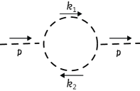
Figure 1: 1-loop thermal self-energy derived three point scalar interaction model

At the one-loop level the thermal self-energy is diagrammatically represented in Fig. 1, and is calculated as

$$i\Sigma_{B,1-loop}^{\gamma_{1}\gamma_{2}}(t_{z_{1}},t_{z_{2}};\mbox{\boldmath$p$})$$

$$=-\frac{1}{2}\int\frac{d^{3}\mbox{\boldmath$k$}_{1}}{(2\pi)^{3}}\frac{d^{3}\mbox{\boldmath$k$}_{2}}{(2\pi)^{3}}(2\pi)^{3}\delta^{(3)}(\mbox{\boldmath$p$}-\mbox{\boldmath$k$}_{1}+\mbox{\boldmath$k$}_{2})$$

$$~{}~{}\times\tau_{3}^{\gamma_{1}\delta}\lambda^{\delta}\{D_{0}(t_{z_{1}},t_{z_{2}};\mbox{\boldmath$k$}_{1})\tau_{3}\}^{\delta\gamma_{2}}\lambda^{\gamma_{2}}\{D_{0}(t_{z_{2}},t_{z_{1}};\mbox{\boldmath$k$}_{2})\tau_{3}\}^{\gamma_{2}\delta}$$

$$=-\frac{\lambda^{2}}{2}\sum^{2}_{i_{1}=1}\sum^{2}_{i_{2}=1}\int\frac{d^{3}\mbox{\boldmath$k$}_{1}}{(2\pi)^{3}}\frac{d^{3}\mbox{\boldmath$k$}_{2}}{(2\pi)^{3}}\frac{1}{4\omega_{k_{1}}\omega_{k_{2}}}(2\pi)^{3}\delta^{(3)}(\mbox{\boldmath$p$}-\mbox{\boldmath$k$}_{1}+\mbox{\boldmath$k$}_{2})$$

$$\times\Biggl{[}\theta(t_{z_{1}}-t_{z_{2}})\ e^{i(E_{k_{1},i_{1}}+E_{k_{2},i_{2}})(t_{z_{1}}-t_{z_{2}})}$$

$$\ \ \ \ \ \times\left(\begin{array}[]{cc}f_{k_{1},i_{1}}(t_{z_{2}})f_{k_{2},i_{2}}(t_{z_{2}})&-\bar{f}_{k_{1},i_{1}}(t_{z_{2}})\bar{f}_{k_{2},i_{2}}(t_{z_{2}})\\ f_{k_{1},i_{1}}(t_{z_{2}})f_{k_{2},i_{2}}(t_{z_{2}})&-\bar{f}_{k_{1},i_{1}}(t_{z_{2}})\bar{f}_{k_{2},i_{2}}(t_{z_{2}})\\ \end{array}\right)$$ (132)

$$\ \ +\theta(t_{z_{2}}-t_{z_{1}})\ e^{-i(E_{k_{1},i_{1}}+E_{k_{2},i_{2}})(t_{z_{1}}-t_{z_{2}})}$$

$$\ \ \ \ \ \times\left(\begin{array}[]{cc}f_{k_{1},i_{1}}(t_{z_{1}})f_{k_{2},i_{2}}(t_{z_{1}})&-f_{k_{1},i_{1}}(t_{z_{1}})f_{k_{2},i_{2}}(t_{z_{1}})\\ \bar{f}_{k_{1},i_{1}}(t_{z_{1}})\bar{f}_{k_{2},i_{2}}(t_{z_{1}})&-\bar{f}_{k_{1},i_{1}}(t_{z_{1}})\bar{f}_{k_{2},i_{2}}(t_{z_{1}})\\ \end{array}\right)\Biggr{]},$$ (135)

where

$$E_{q,1}=\omega_{q},\ \ E_{q,2}=-\omega_{q},$$ (136)

$$f_{q,1}(t)=n_{q}(t),\ \ \ f_{q,2}(t)=1+n_{q}(t),$$ (137)

$$\bar{f}_{q,1}(t)=1+n_{q}(t),\ \ \ \bar{f}_{q,2}(t)=n_{q}(t).$$ (138)

Thus the off-diagonal elements, (110) and (113), are given by

$$\lim_{t_{x}\rightarrow t_{y}}\int dt_{z_{1}}dt_{z_{2}}\delta\Sigma_{B,1}(t_{x},t_{z_{1}},t_{z_{2}},t_{y};\mbox{\boldmath$p$})$$

$$=\lim_{t_{x}\rightarrow t_{y}}\int dt_{z_{1}}dt_{z_{2}}\delta\Sigma_{B,4}(t_{x},t_{z_{1}},t_{z_{2}},t_{y};\mbox{\boldmath$p$})$$

$$=\int_{-\infty}^{t_{x}}dt_{s}\frac{1}{2\omega_{p}}\sum^{2}_{i_{1}=1}\sum^{2}_{i_{2}=1}\frac{\lambda^{2}}{2}\int\frac{d^{3}\mbox{\boldmath$k$}_{1}}{(2\pi)^{3}}\frac{d^{3}\mbox{\boldmath$k$}_{2}}{(2\pi)^{3}}\frac{1}{4\omega_{p}\omega_{k_{1}}\omega_{k_{2}}}(2\pi)^{3}\delta^{(3)}(\mbox{\boldmath$p$}-\mbox{\boldmath$k$}_{1}+\mbox{\boldmath$k$}_{2})$$

$$\ \ \times\frac{{\rm sin}\{(\omega_{p}+E_{k_{1},i_{1}}+E_{k_{2},i_{2}})(t_{x}-t_{s})\}}{\omega_{p}+E_{k_{1},i_{1}}+E_{k_{2},i_{2}}}$$

$$\ \times\Bigl{\{}n_{p}(t_{s})f_{k_{1},i_{1}}(t_{s})f_{k_{2},i_{2}}(t_{s})-(1+n_{p}(t_{s}))\bar{f}_{k_{1},i_{1}}(t_{s})\bar{f}_{k_{2},i_{2}}(t_{s})\Bigr{\}},$$ (139)

at the equal time limit. When the Bose distribution function is assumed for $n_{p}(t)$, Eq. (139) vanishes. It shows that the Bose distribution is a stationary solution for Eq. (116).

Inserting Eq. (139) into Eq. (116), we obtain the time evolution equation for the thermal Bogoliubov parameter,

$$\dot{n}_{p}(t_{x})=-\frac{\lambda^{2}}{2}\sum^{2}_{i_{1}=1}\sum^{2}_{i_{2}=1}\int_{-\infty}^{t_{x}}dt_{s}\int\frac{d^{3}\mbox{\boldmath$k$}_{1}}{(2\pi)^{3}}\frac{d^{3}\mbox{\boldmath$k$}_{2}}{(2\pi)^{3}}\frac{1}{4\omega_{p}\omega_{k_{1}}\omega_{k_{2}}}$$

$$~{}\times{\cos}\{(\omega_{p}+E_{k_{1},i_{1}}+E_{k_{2},i_{2}})(t_{x}-t_{s})\}(2\pi)^{3}\delta^{(3)}(\mbox{\boldmath$p$}-\mbox{\boldmath$k$}_{1}+\mbox{\boldmath$k$}_{2})$$

$$~{}\times\Bigl{\{}n_{p}(t_{s})f_{k_{1},i_{1}}(t_{s})f_{k_{2},i_{2}}(t_{s})-(1+n_{p}(t_{s}))\bar{f}_{k_{1},i_{1}}(t_{s})\bar{f}_{k_{2},i_{2}}(t_{s})\Bigr{\}}.$$ (140)

The third line of this equation has the same statistical structure as the quantum Boltzmann equation. Off-shell contribution is included through the second line of Eq. (140).

At the limit, $t_{x}\rightarrow\infty$, the second line of Eq. (139) reduces to the delta function which guarantees the energy conservation. Then the collision term of the quantum Boltzmann equation is derived from Eq. (139). It shows that time evolution for the thermal Bogoliubov parameter is described by the quantum Boltzmann equation at the limit.

5.2 $\lambda\phi^{4}$ interaction model

Next we consider a neutral scalar field with a four-point self-interaction. The model is defined by the Hamiltonian,

$$\hat{H}=H-\tilde{H},$$ (141)

with

$$H=\int d^{3}\mbox{\boldmath$x$}\Bigl{[}\frac{1}{2}\bigl{\{}\pi_{a}(x)^{2}+\phi_{a}(x)(-\nabla_{x}^{2}+m^{2})\phi_{a}(x)\bigr{\}}+\frac{\lambda}{4!}\phi_{a}(x)^{4}\Bigr{]}.$$ (142)

The numerical factor in the interaction term provides the same assignment to each vertex as in the previous model.

We calculate the thermal self-energy in this model.

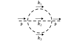
Figure 2: 2-loop thermal self-energy in $\lambda\phi^{4}$ interaction model

Since there is no momentum transfer from the external to the internal lines, the self-energy has a diagonal form at the one-loop level. Thus the self-consistency renormalization condition is satisfied for $\dot{n}_{p}(t)=0$ at one-loop level. The time evolution of the thermal Bogoliubov parameter is induced from the two-loop self-energy illustrated in Fig. 2. We compute the diagram and obtain

$$i\Sigma_{B,2-loop}^{\gamma_{1}\gamma_{2}}(t_{z_{1}},t_{z_{2}};\mbox{\boldmath$p$})$$

$$=-\frac{1}{3!}\int\frac{d^{3}\mbox{\boldmath$k$}_{1}}{(2\pi)^{3}}\frac{d^{3}\mbox{\boldmath$k$}_{2}}{(2\pi)^{3}}\frac{d^{3}\mbox{\boldmath$k$}_{3}}{(2\pi)^{3}}(2\pi)^{3}\delta^{(3)}(\mbox{\boldmath$p$}-\mbox{\boldmath$k$}_{1}-\mbox{\boldmath$k$}_{2}-\mbox{\boldmath$k$}_{3})$$

$$\times\tau_{3}^{\gamma_{1}\delta}\lambda^{\delta}\{D_{0}(t_{z_{1}},t_{z_{2}};\mbox{\boldmath$k$}_{1})\tau_{3}\}^{\delta\gamma_{2}}\{D_{0}(t_{z_{1}},t_{z_{2}};\mbox{\boldmath$k$}_{2})\tau_{3}\}^{\delta\gamma_{2}}\{D_{0}(t_{z_{1}},t_{z_{2}};\mbox{\boldmath$k$}_{3})\tau_{3}\}^{\delta\gamma_{2}}\lambda^{\gamma_{2}}$$

$$=-\frac{\lambda^{2}}{3!}\sum^{2}_{i_{1}=1}\sum^{2}_{i_{2}=1}\sum^{2}_{i_{3}=1}\int\frac{d^{3}\mbox{\boldmath$k$}_{1}}{(2\pi)^{3}}\frac{d^{3}\mbox{\boldmath$k$}_{2}}{(2\pi)^{3}}\frac{d^{3}\mbox{\boldmath$k$}_{3}}{(2\pi)^{3}}\frac{1}{8\omega_{k_{1}}\omega_{k_{2}}\omega_{k_{3}}}(2\pi)^{3}\delta^{(3)}(\mbox{\boldmath$p$}-\mbox{\boldmath$k$}_{1}-\mbox{\boldmath$k$}_{2}-\mbox{\boldmath$k$}_{3})$$

$$\times\Biggl{[}\theta(t_{z_{1}}-t_{z_{2}})e^{i(E_{k_{1},i_{1}}+E_{k_{2},i_{2}}+E_{k_{3},i_{3}})(t_{z_{1}}-t_{z_{2}})}$$ (148)

$$\times\left(\begin{array}[]{cc}f_{k_{1},i_{1}}(t_{z_{2}})f_{k_{2},i_{2}}(t_{z_{2}})f_{k_{3},i_{3}}(t_{z_{2}})&-\bar{f}_{k_{1},i_{1}}(t_{z_{2}})\bar{f}_{k_{2},i_{2}}(t_{z_{2}})\bar{f}_{k_{3},i_{3}}(t_{z_{2}})\\ f_{k_{1},i_{1}}(t_{z_{2}})f_{k_{2},i_{2}}(t_{z_{2}})f_{k_{3},i_{3}}(t_{z_{2}})&-\bar{f}_{k_{1},i_{1}}(t_{z_{2}})\bar{f}_{k_{2},i_{2}}(t_{z_{2}})\bar{f}_{k_{3},i_{3}}(t_{z_{2}})\\ \end{array}\right)$$

$$\ \ \ +\theta(t_{z_{2}}-t_{z_{1}})e^{-i(E_{k_{1},i_{1}}+E_{k_{2},i_{2}}+E_{k_{3},i_{3}})(t_{z_{1}}-t_{z_{2}})}$$

$$\times\left(\begin{array}[]{cc}f_{k_{1},i_{1}}(t_{z_{1}})f_{k_{2},i_{2}}(t_{z_{1}})f_{k_{3},i_{3}}(t_{z_{1}})&-f_{k_{1},i_{1}}(t_{z_{1}})f_{k_{2},i_{2}}(t_{z_{1}})f_{k_{3},i_{3}}(t_{z_{1}})\\ \bar{f}_{k_{1},i_{1}}(t_{z_{1}})\bar{f}_{k_{2},i_{2}}(t_{z_{1}})\bar{f}_{k_{3},i_{3}}(t_{z_{1}})&-\bar{f}_{k_{1},i_{1}}(t_{z_{1}})\bar{f}_{k_{2},i_{2}}(t_{z_{1}})\bar{f}_{k_{3},i_{3}}(t_{z_{1}})\\ \end{array}\right)\Biggr{]}.$$

The off-diagonal elements, (110) and (113), are given by

$$\lim_{t_{x}\rightarrow t_{y}}\int dt_{z_{1}}dt_{z_{2}}\delta\Sigma_{B,1}(t_{x},t_{z_{1}},t_{z_{2}},t_{y};\mbox{\boldmath$p$})$$

$$=\lim_{t_{x}\rightarrow t_{y}}\int dt_{z_{1}}dt_{z_{2}}\delta\Sigma_{B,4}(t_{x},t_{z_{1}},t_{z_{2}},t_{y};\mbox{\boldmath$p$})$$

$$=\int_{-\infty}^{t_{x}}dt_{s}\frac{1}{2\omega_{p}}\frac{\lambda^{2}}{3!}\sum^{2}_{i_{1}=1}\sum^{2}_{i_{2}=1}\sum^{2}_{i_{3}=1}\int\frac{d^{3}\mbox{\boldmath$k$}_{1}}{(2{\pi})^{3}}\frac{d^{3}\mbox{\boldmath$k$}_{2}}{(2{\pi})^{3}}\frac{d^{3}\mbox{\boldmath$k$}_{3}}{(2{\pi})^{3}}\frac{1}{8\omega_{p}\omega_{k_{1}}\omega_{k_{2}}\omega_{k_{3}}}$$

$$\times\frac{{\rm sin}\bigl{\{}(\omega_{p}+E_{k_{1},i_{1}}+E_{k_{2},i_{2}}+E_{k_{3},i_{3}})(t_{x}-t_{s})\bigr{\}}}{\omega_{p}+E_{k_{1},i_{1}}+E_{k_{2},i_{2}}+E_{k_{3},i_{3}}}(2\pi)^{3}\delta^{(3)}(\mbox{\boldmath$p$}-\mbox{\boldmath$k$}_{1}-\mbox{\boldmath$k$}_{2}-\mbox{\boldmath$k$}_{3})$$

$$\times\Bigl{[}n_{p}(t_{s})f_{k_{1},i_{1}}(t_{s})f_{k_{2},i_{2}}(t_{s})f_{k_{3},i_{3}}(t_{s})-(1+n_{p}(t_{s}))\bar{f}_{k_{1},i_{1}}(t_{s})\bar{f}_{k_{2},i_{2}}(t_{s})\bar{f}_{k_{3},i_{3}}(t_{s})\Bigr{]},$$

(149)

at the equal time limit. Substituting Eq. (149) to Eq. (116), we obtain the time evolution equation for the thermal Bogoliubov parameter,

$$\dot{n}_{p}(t_{x})=(-1)\frac{\lambda^{2}}{3!}\sum^{2}_{i_{1}=1}\sum^{2}_{i_{2}=1}\sum^{2}_{i_{3}=1}\int_{-\infty}^{t_{x}}dt_{s}\int\frac{d^{3}\mbox{\boldmath$k$}_{1}}{(2{\pi})^{3}}\frac{d^{3}\mbox{\boldmath$k$}_{2}}{(2{\pi})^{3}}\frac{d^{3}\mbox{\boldmath$k$}_{3}}{(2{\pi})^{3}}\frac{1}{8\omega_{p}\omega_{k_{1}}\omega_{k_{2}}\omega_{k_{3}}}$$

$$\times{\cos}\bigl{\{}(\omega_{p}+E_{k_{1},i_{1}}+E_{k_{2},i_{2}}+E_{k_{3},i_{3}})(t_{x}-t_{s})\bigr{\}}(2\pi)^{3}\delta^{(3)}(\mbox{\boldmath$p$}-\mbox{\boldmath$k$}_{1}-\mbox{\boldmath$k$}_{2}-\mbox{\boldmath$k$}_{3})$$

$$\times\Bigl{[}n_{p}(t_{s})f_{k_{1},i_{1}}(t_{s})f_{k_{2},i_{2}}(t_{s})f_{k_{3},i_{3}}(t_{s})-(1+n_{p}(t_{s}))\bar{f}_{k_{1},i_{1}}(t_{s})\bar{f}_{k_{2},i_{2}}(t_{s})\bar{f}_{k_{3},i_{3}}(t_{s})\Bigr{]}.$$

(150)

This equation has the same statistical structure as the quantum Boltzmann equation for the $\lambda\phi^{4}$ interaction model. It should be noticed that a coefficient of the right-hand side in Eq. (150) is twice of the one obtained in Ref. SD-2. As is shown in Appendix B, Eq. (150) coincides with the quantum transport equation in the non-relativistic regime[19].

6 Conclusion

We have investigated a relativistic neutral scalar field in NETFD. Thermal degree of freedom is introduced through the time dependent Bogoliubov transformation. Then the thermal counter term has to be introduced for a consistent description of both $a(t)$ and $\xi(t)$ under the transformation, and is a part of the interaction Hamiltonian. We adopt the perturbative expansion, and calculate the full propagator in the canonical formalism. The Bogoliubov matrix structure of the propagator is crucial.

Applying the self-consistency renormalization condition[24] to a relativistic neutral scalar field, we have derived the time evolution equation for the thermal Bogoliubov parameter which is considered to be the particle number density. It has been shown that the equation reduces to the quantum Boltzmann equation in $\phi^{3}$ and $\phi^{4}$ interaction models.

In this paper we impose the Lorentz covariance for the neutral scalar field and decompose it in terms of the creation and annihilation operators, $\xi$ and $\xi^{\dagger}$. It is not always possible to do so in a general situation of non-equilibrium system. Some modification would be necessary to apply the procedure to a field with a time-dependent screening mass, for example.

There are some remaining problems. There is no counter term for the second and third lines in Eq. (85). These terms may have a nontrivial contribution to the time evolution equation at higher order. @ In the present paper we have assumed spatial homogeneity. The space-time dependence is also important to study some relativistic systems. Some works to extend NETFD to spatially inhomogeneous systems have been attempted for non-relativistic field. An essence of such extension is to expand the field operator not by a complete set of plane wave functions, but by a complete set mixing momentum for diffusion process[15, 16] or by a complete set of wave functions under trapping potential for cold atomic system[19, 20], while the equal-time commutation relations are preserved. We can formulate inhomogeneous TFD for relativistic fields in similar ways. We are also interested in applying the procedure to a relativistic Dirac field and an inhomogeneous system. We hope to solve these problems and report the result in future.

Appendix A Propagator for a free neutral scalar field

In TFD the Feynman propagator for a free neutral scalar field is given by the expectation value of the time ordered product of two scalar fields. It has the $2\times 2$ matrix form in the thermal doublet notation,[4]

$$D_{0}^{\alpha\beta}(t_{x},t_{y},\mbox{\boldmath$x$}-\mbox{\boldmath$y$})\equiv\langle\theta|T[\phi_{a}^{\alpha}(x)\bar{\phi}_{a}^{\beta}(y)]|\theta\rangle,$$ (151)

where the neutral scalar fields, $\phi_{a}$ and $\bar{\phi}_{a}$, are decomposed into the positive and negative frequency parts by Eqs. (52) and (53). The thermal Bogoliubov transformation is applied, then the propagator (151) reads

$$D_{0}^{\alpha\beta}(t_{x},t_{y},\mbox{\boldmath$x$}-\mbox{\boldmath$y$})$$

$$=\theta(t_{x}-t_{y})\Bigl{[}B^{-1}(n_{|\nabla_{x}|}(t_{x}))^{\alpha\gamma_{1}}\langle\theta|\phi_{\xi,+}^{\gamma_{1}}(x)\bar{\phi}_{\xi,-}^{\gamma_{2}}(y)|\theta\rangle B(n_{|\overleftarrow{\nabla}_{y}|}(t_{y}))^{\gamma_{2}\beta}$$

$$~{}~{}+\{\tau_{3}B(n_{|\nabla_{x}|}(t_{x}))^{T}\}^{\alpha\gamma_{1}}\langle\theta|\phi_{\xi,-}^{\gamma_{1}}(x)\bar{\phi}_{\xi,+}^{\gamma_{2}}(y)|\theta\rangle\{\tau_{3}B^{-1}(n_{|\overleftarrow{\nabla}_{y}|}(t_{y}))^{T}\}^{\gamma_{2}\beta}\Bigr{]}$$

$$~{}+\theta(t_{y}-t_{x})\Bigl{[}B^{-1}(n_{|\nabla_{x}|}(t_{x}))^{\alpha\gamma_{1}}\langle\theta|\bar{\phi}_{\xi,-}^{\gamma_{2}}(y)\phi_{\xi,+}^{\gamma_{1}}(x)|\theta\rangle B(n_{|\overleftarrow{\nabla}_{y}|}(t_{y}))^{\gamma_{2}\beta}$$

$$~{}~{}+\{\tau_{3}B(n_{|\nabla_{x}|}(t_{x}))^{T}\}^{\alpha\gamma_{1}}\langle\theta|\bar{\phi}_{\xi,+}^{\gamma_{2}}(y)\phi_{\xi,-}^{\gamma_{1}}(y)|\theta\rangle\{\tau_{3}B^{-1}(n_{|\overleftarrow{\nabla}_{y}|}(t_{y}))^{T}\}^{\gamma_{2}\beta}\Bigr{]},$$ (152)

where the fields, $\phi_{\xi,\pm}$ and $\bar{\phi}_{\xi,\pm}$, are defined in Eq. (73).

Due to the definition of the thermal vacuum (26) and (27) the thermal propagator, $D_{0}^{\alpha\beta}$, reduces to

$$D_{0}^{\alpha\beta}(t_{x},t_{y},\mbox{\boldmath$x$}-\mbox{\boldmath$y$})=\Biggl{[}B^{-1}(n_{|\nabla_{x}|}(t_{x}))^{\alpha\gamma_{1}}D_{0,R}^{\gamma_{1}\gamma_{2}}(x-y)B(n_{|\overleftarrow{\nabla}_{y}|}(t_{y}))^{\gamma_{2}\beta}$$

$$+\{\tau_{3}B(n_{|\nabla_{x}|}(t_{x}))^{T}\}^{\alpha\gamma_{1}}D_{0,A}^{\gamma_{1}\gamma_{2}}(x-y)\{B^{-1}(n_{|\overleftarrow{\nabla}_{y}|}(t_{y}))^{T}\tau_{3}\}^{\gamma_{2}\beta}\Biggr{]},$$ (153)

where $D_{0,R}^{\gamma_{1}\gamma_{2}}(x-y)$ and $D_{0,A}^{\gamma_{1}\gamma_{2}}(x-y)$ represent retarded and advanced parts of the propagator, respectively,

$$D_{0,R}^{11}(x-y)=\int\frac{d^{3}\mbox{\boldmath$p$}}{(2\pi)^{3}}\theta(t_{x}-t_{y})\frac{1}{2\omega_{p}}{\rm e}^{-ip\cdot(x-y)},$$ (154)

$$D_{0,R}^{22}(x-y)=-\int\frac{d^{3}\mbox{\boldmath$p$}}{(2\pi)^{3}}\theta(t_{y}-t_{x})\frac{1}{2\omega_{p}}{\rm e}^{-ip\cdot(x-y)},$$ (155)

$$D_{0,A}^{11}(x-y)=\int\frac{d^{3}\mbox{\boldmath$p$}}{(2\pi)^{3}}\theta(t_{y}-t_{x})\frac{1}{2\omega_{p}}{\rm e}^{ip\cdot(x-y)},$$ (156)

$$D_{0,A}^{22}(x-y)=-\int\frac{d^{3}\mbox{\boldmath$p$}}{(2\pi)^{3}}\theta(t_{x}-t_{y})\frac{1}{2\omega_{p}}{\rm e}^{ip\cdot(x-y)},$$ (157)

$${\rm other\ components}=0.$$

Thus we reproduce the result obtained in Refs. umezawa1 and prop1. The thermal propagator (153) has the same form as the one in an equilibrium system. The time dependence is introduced through the thermal Bogoliubov transformation.

Appendix B Non-relativistic limit of the Boltzmann equation

Here we take the non-relativistic limit of the time evolution equation for the $\lambda\phi^{4}$ interaction model (150) and compare it with the transport equation for the cold atom system.

The cold atom system is described by the Hamiltonian,

$$H=\int d^{3}\mbox{\boldmath$x$}\left[-\psi^{\dagger}(x)\frac{\nabla_{x}^{2}}{2m}\psi(x)+\frac{g}{2}\psi^{\dagger}(x)\psi^{\dagger}(x)\psi(x)\psi(x)\right],$$ (158)

where $\psi$ represents a non-relativistic scalar field,

$$\psi(x)=\int\frac{d^{3}\mbox{\boldmath$p$}}{(2\pi)^{3}}a_{p}(t_{x})e^{i\mbox{\boldmath$p$}\cdot\mbox{\boldmath$x$}}.$$ (159)

The quantum transport equation for this system is given by[19]

$$\dot{n}_{p}(t)=4g^{2}{\rm Re}\int_{-\infty}^{t}ds\int\frac{d^{3}\mbox{\boldmath$p$}_{1}}{(2\pi)^{3}}\frac{d^{3}\mbox{\boldmath$p$}_{2}}{(2\pi)^{3}}\frac{d^{3}\mbox{\boldmath$p$}_{3}}{(2\pi)^{3}}$$

$$\times(2\pi)^{3}\delta^{(3)}(\mbox{\boldmath$p$}_{1}+\mbox{\boldmath$p$}_{2}-\mbox{\boldmath$p$}_{3}-\mbox{\boldmath$p$})e^{-i(\varepsilon_{p_{1}}+\varepsilon_{p_{2}}-\varepsilon_{p_{3}}-\varepsilon_{p})(t-s)}$$

$$\times\Bigr{\{}n_{p_{1}}(s)n_{p_{2}}(s)(1+n_{p_{3}}(s))(1+n_{p}(s))-(1+n_{p_{1}}(s))(1+n_{p_{2}}(s))n_{p_{3}}(s)n_{p}(s)\Bigr{\}},$$

(160)

where $\varepsilon_{p}$ is the kinetic energy for the non-relativistic field,

$$\varepsilon_{p}=\frac{\mbox{\boldmath$p$}^{2}}{2m}.$$ (161)

At the non-relativistic limit, $|\mbox{\boldmath$p$}|\ll m$, the energy eigenvalue $\omega_{p}$ reduces to

$$\omega_{p}\approx m+\varepsilon_{p}.$$ (162)

We restrict the momentum for the scalar field in $-p_{\epsilon}\leq p_{i}\leq p_{\epsilon}$ with a cut-off parameter, $0<p_{\epsilon}\ll m$. Thus the relativistic scalar field, $\phi_{a}$, is decomposed to be

$$\phi_{a}(x)\approx\int_{-p_{\epsilon}}^{p_{\epsilon}}\frac{d^{3}\mbox{\boldmath$p$}}{(2\pi)^{3}}\frac{1}{\sqrt[]{2m}}\bigl{\{}a_{p}(t_{x})e^{i\mbox{\boldmath$p$}\cdot\mbox{\boldmath$x$}}+a_{p}^{\dagger}(t_{x})e^{-i\mbox{\boldmath$p$}\cdot\mbox{\boldmath$x$}}\bigr{\}}$$

$$=\phi_{a,+}(x)+\phi_{a,-}(x),$$ (163)

where $\phi_{a,+}$ and $\phi_{a,-}$ indicate the positive and negative frequency parts.

The interaction for the cold atom system (158) can be identified with the interaction, $\phi_{a,+}\phi_{a,+}\phi_{a,-}\phi_{a,-}$. There are six corresponding terms in the interaction, $\lambda\phi_{a}^{4}$. Thus we obtain the following correspondence between the interaction terms for the cold atom system and the $\lambda\phi_{a}^{4}$ model in the non-relativistic regime,

$$\frac{g}{2}\psi^{\dagger}(x)\psi^{\dagger}(x)\psi(x)\psi(x)=6\frac{\lambda}{4!}\phi_{a,+}(x)\phi_{a,+}(x)\phi_{a,-}(x)\phi_{a,-}(x),$$ (164)

We find that there is a correspondence if we make a replacement

$$\lambda\leftrightarrow 8m^{2}g.$$ (165)

Since the transport equation (160) comes from the two-body scattering, we pick up terms which represent the two-body scattering in Eq. (150). Hence Eq. (150) is rewritten as

$$\dot{n}_{p}(t_{x})=\frac{\lambda^{2}}{2}\int_{-\infty}^{t_{x}}dt_{s}\int\frac{d^{3}\mbox{\boldmath$k$}_{1}}{(2{\pi})^{3}}\frac{d^{3}\mbox{\boldmath$k$}_{2}}{(2{\pi})^{3}}\frac{d^{3}\mbox{\boldmath$k$}_{3}}{(2{\pi})^{3}}\frac{1}{8\omega_{p}\omega_{k_{1}}\omega_{k_{2}}\omega_{k_{3}}}$$

$$\times{\cos}\bigl{\{}(\omega_{p}+\omega_{k_{1}}-\omega_{k_{2}}-\omega_{k_{3}})(t_{x}-t_{s})\bigr{\}}(2\pi)^{3}\delta^{(3)}(\mbox{\boldmath$p$}-\mbox{\boldmath$k$}_{1}-\mbox{\boldmath$k$}_{2}-\mbox{\boldmath$k$}_{3})$$

$$\times\Bigl{[}n_{p}(t_{s})n_{k_{1}}(t_{s})(1+n_{k_{2}}(t_{s}))(1+n_{k_{3}}(t_{s}))-(1+n_{p}(t_{s}))(1+n_{k_{1}}(t_{s}))n_{k_{2}}(t_{s})n_{k_{3}}(t_{s})\Bigr{]}.$$

(166)

Substituting (162) and (165) into Eq. (166) we obtain the quantum Boltzmann equation in the non-relativistic regime,

$$\dot{n}_{p}(t_{x})=4g^{2}\int_{-\infty}^{t_{x}}dt_{s}\int\frac{d^{3}\mbox{\boldmath$k$}_{1}}{(2{\pi})^{3}}\frac{d^{3}\mbox{\boldmath$k$}_{2}}{(2{\pi})^{3}}\frac{d^{3}\mbox{\boldmath$k$}_{3}}{(2{\pi})^{3}}$$

$$\times{\cos}\bigl{\{}(\varepsilon_{p}+\varepsilon_{k_{1}}-\varepsilon_{k_{2}}-\varepsilon_{k_{3}})(t_{x}-t_{s})\bigr{\}}(2\pi)^{3}\delta^{(3)}(\mbox{\boldmath$p$}-\mbox{\boldmath$k$}_{1}-\mbox{\boldmath$k$}_{2}-\mbox{\boldmath$k$}_{3})$$

$$\times\Bigl{[}n_{p}(t_{s})n_{k_{1}}(t_{s})(1+n_{k_{2}}(t_{s}))(1+n_{k_{3}}(t_{s}))-(1+n_{p}(t_{s}))(1+n_{k_{1}}(t_{s}))n_{k_{2}}(t_{s})n_{k_{3}}(t_{s})\Bigr{]}.$$

(167)

In homogeneous system the quantum Boltzmann equation (167) and Eq. (160) become identical. Therefore the time evolution equation (150) is consistent with the quantum transport equation (160).

References

• [1] I. Senitzky, Phys. Rev. 119 (1960), 670.
• [2] K. Chou, Z. Su, B. Hao and L. Yu, \PRP118,1985,1.
• [3] E. Calzetta and B. Hu, \PRD37,1988,2878.
• [4] H. Umezawa, ADVANCED FIELD THEORY Micro, Macro, and Thermal Physics (American Institute of Physics, 1995).
• [5] Y. Takahashi and H. Umezawa, Collective Phenomena 2 (1975), 55.
• [6] T. Arimitsu and H. Umezawa, \PTP77,1987,53.
• [7] T. Arimitsu, H. Umezawa and Y. Yamanaka, J. Math. Phys. 28 (1987), 2741.
• [8] T. Arimitsu and H. Umezawa, \PTP74,1985,429.
• [9] H. Matsumoto, \PTP80,1988,57.
• [10] H. Umezawa and Y. Yamanaka, Advances in Physics 37 (1988), 531.
• [11] I. Hardman, H. Umezawa and Y. Yamanaka, \PLA146,1990,293.
• [12] T. Evans, I. Hardman, H. Umezawa and Y. Yamanaka, Fortschr. Phys. 41 (1993), 151.
• [13] H. Umezawa and Y. Yamanaka, Mod. Phys. Lett. A 7 (1992), 3509.
• [14] Y. Yamanaka, H. Umezawa, K. Nakamura and T. Arimitsu, Int. J. Mod. Phys. A 9 (1994), 1153.
• [15] K. Nakamura, H. Umezawa, and Y. Yamanaka, Mod. Phys. Lett. A 7 (1992), 3583.
• [16] Y. Yamanaka and K. Nakamura, Mod. Phys. Lett. A 9 (1994), 2879.
• [17] H. Matsumoto and S. Sakamoto, \PTP105,2001,573.
• [18] H. Matsumoto and S. Sakamoto, \PTP107,2002,689.
• [19] Y. Nakamura, T. Sunaga, M. Mine, M. Okumura, Y. Yamanaka, \ANN325,2010,426.
• [20] Y. Nakamura, Y. Yamanaka, \ANN326,2011,1070.
• [21] H. Matsumoto, Physica A 158 (1989), 291.
• [22] P. Henning, \PRP253,1995,235.
• [23] T. Evans, I. Hardman, H. Umezawa and Y. Yamanaka, J. Math. Phys. 33 (1992), 370.
• [24] H. Chu and H. Umezawa, Int. J. Mod. Phys. A 10 (1995), 1693.
• [25] H. Chu and H. Umezawa, \PLA177,1993,385.
• [26] Y. Mizutani and T. Inagaki, \PTP125,2011,933.