CH abundance gradient in TMC-1

Abstract

Aims. The aim of this study is to examine if the well-known chemical gradient in TMC-1 is reflected in the amount of rudimentary forms of carbon available in the gas-phase. As a tracer we use the CH radical which is supposed to be well correlated with carbon atoms and simple hydrocarbon ions.

Methods. We observed the 9-cm $\Lambda$-doubling lines of CH along the dense filament of TMC-1. The CH column densities were compared with the total H₂ column densities derived using the 2MASS NIR data and previously published SCUBA maps and with OH column densities derived using previous observations with Effelsberg. We also modelled the chemical evolution of TMC-1 adopting physical conditions typical of dark clouds using the UMIST Database for Astrochemistry gas-phase reaction network to aid the interpretation of the observed OH/CH abundance ratios.

Results. The CH column density has a clear peak in the vicinity of the cyanopolyyne maximum of TMC-1. The fractional CH abundance relative to H₂ increases steadily from the northwestern end of the filament where it lies around $1.0\,10^{-8}$, to the southeast where it reaches a value of $\leavevmode\nobreak\ 2.0\,10^{-8}$. The OH and CH column densities are well correlated, and we obtained OH/CH abundance ratios of $\sim 16-20$. These values are clearly larger than what has been measured recently in diffuse interstellar gas and is likely to be related to C to CO conversion at higher densities. The good correlation between CH and OH can be explained by similar production and destruction pathways. We suggest that the observed CH and OH abundance gradients are mainly due to enhanced abundances in a low-density envelope which becomes more prominent in the southeastern part and seems to continue beyond the dense filament.

Conclusions. An extensive envelope probably signifies an early stage of dynamical evolution, and conforms with the detection of a large CH abundance in the southeastern part of the cloud. The implied presence of other simple forms of carbon in the gas phase provides a natural explanation for the observation of “early-type” molecules in this region.

1 Introduction

The 9-cm $\Lambda$-doubling lines of the methylidyne radical CH have been commonly used to trace low density gas in diffuse clouds and at the edges of dense clouds. Observational surveys have demonstrated a linear correlation between the CH column density and visual extiction (and thereby also $N({\rm H_{2}})$) in low-extinction molecular clouds (e.g. Hjalmarson et al. 1977; Mattila 1986; Magnani & Onello 1993; Magnani et al. 2005). On the other hand, CH is likely to be critically dependent on the presence of free carbon in the gas phase. The modelling results of Flower et al. (1994) predict that CH (or CN) can trace atomic carbon content even in the cloud interiors. While the fine structure lines of C I become easily optically thick and dominated by the outer layers of the cloud, the ground state CH lines are optically thin. Therefore one can hope to “see” through the cloud in these lines, even if the cloud edges may have a significant contribution, and the CH abundance is likely to vary as a function of density.

We have made observations of the $\Lambda$-doubling transitions of CH in its ground state along the dense filament of Taurus Molecular Cloud-1 (TMC-1). With the aid of these observations we examine the predicted correlation of atomic carbon and cyanopolyynes and other unsaturated carbon-chain molecules in TMC-1.

According to most chemistry models adopted for TMC-1 the cyanopolyyne (CP) peak in its southeastern end should represent an early stage of chemical evolution and have a high concentration of carbon in the form of C or C⁺ (e.g. Hirahara et al. 1992; Hartquist et al. 1996; Pratap et al. 1997). Alternative views have been presented by Hartquist et al. (1996) who discuss the possibility that the CP peak is highly depleted and represents a chemically more advanced stage than the NH₃ peak, and by Markwick et al. (2000, 2001) who suggest that carbon chemistry at the CP peak has been revived by evaporation of carbon bearing mantle species (CH₄, C₂H₂, C₂H₄) following grain-grain collisions induced by the ion-neutral slip produced by the passge of an Alfvén wave. In this model, complex organic species are not necessarily coincident with the most rudimentary forms of carbon.

Previous C I 492 GHz fine structure line observations of Schilke et al. (1995) and Maezawa et al. (1999) indicate high abundances neutral carbon in the direction of TMC-1. In their mapping of Heiles Cloud 2 (including TMC-1), Maezawa et al. estimate that the C I/CO abundance ratio towards the CP peak is about 0.1, and that the ratio increases to $\sim 1$ in the ”C I peak” on the southern side of the cloud. These estimates are, however, uncertain because of the unknown optical thickness and excitation temperature of the 492 GHz C I line. The TMC-1 ridge is not visible on the C I map which is dominated by emission from more diffuse gas.

In the present paper, we derive the fractional abundances of CH along an axis aligned with the dense filament of TMC-1 and going through the CP peak. The molecular hydrogen column densities, $N({\rm H_{2}})$, required for this purpose, are estimated by combining an extinction map derived from the 2MASS data with JCMT/SCUBA dust continuum maps at 850 and 450 $\mu$m presented in Nutter et al. (2008). The CH observations are described in Sect. 2, and in Sect. 3 the CH and H₂ column densities are derived. In Sect. 4 we compare the new data with previous observations, and discuss the chemical implications of the obtained CH abundances. Finally, in Sect. 5 we summarize our conclusions.

2 Observations

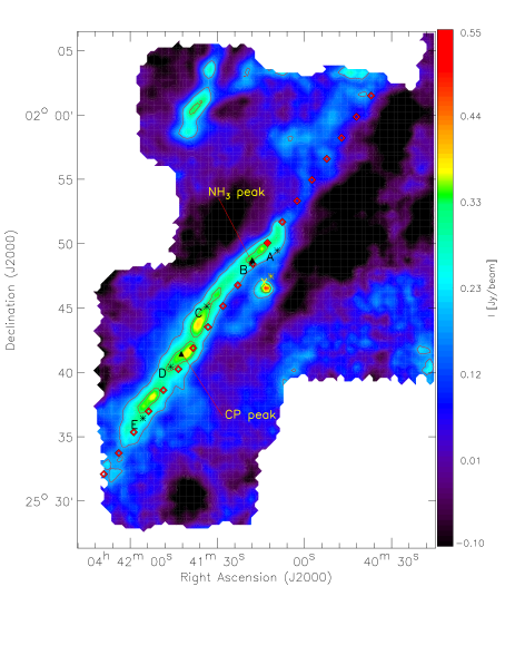
(a)

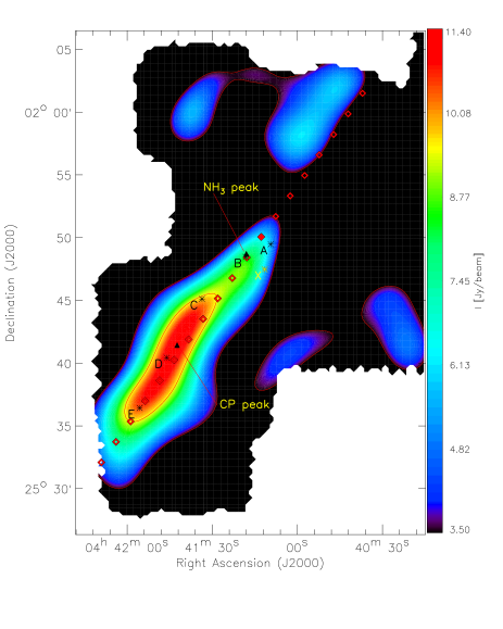
(b)

Figure 1: TMC-1 as seen by SCUBA at $850\ \rm{\mu m}$ (convolved to $30\arcsec$ in a and $228\arcsec$ in b). The map is reproduced from Nutter et al. (2008), who calls the filament “the Bull’s Tail”. The red diamonds represent the locations of our CH spectral observations (separated by $2\arcmin$), and the black triangles mark the locations of the cyanopolyyne and ammonia maxima. The letters A-E and X mark the regions of the six dense cores as per Hirahara et al. (1992), with the asterisks marking the locations of the CCS maxima corresponding to the six cores. The two contour line levels correspond to intensities of 0.19 and 0.32 Jy/beam on the $30\arcsec$ resolution map and 3.5 and 9.6 Jy/beam on the $228\arcsec$ map. The filled red diamond on the image is located at $\alpha_{\rm{J2000}}=04^{\rm{h}}41^{\rm{m}}12\aas@@fstack{s}7$, $\delta_{\rm{J2000}}=25\degr 50\arcmin 04\arcsec$, marking the origin of the CH observations performed by us.

2.1 CH spectra

The $\Lambda$-doubling line of CH in the ${}^{2}\Pi_{1/2},J=1/2$ ground state ($\lambda=9\ \rm{cm}$) was observed in August 2003 using the 100-m radio telescope, located in Effelsberg, Germany, belonging to the Max-Planck-Institut f$\rm{\ddot{u}}$r Radioastronomie. The acquired data includes observations of the main spectral line 1-1 and the satellite lines 1-0 and 0-1. The frequency is $3335.481\ \rm{MHz}$ for the main line, $3263.794\ \rm{MHz}$ and $3349.193\ \rm{MHz}$ for the lower and upper satellites. The FWHM of the antenna at these frequencies is approximately $3\arcmin.8$. During the observations the system temperature varied approximately between $55\ \rm{K}$ and $60\ \rm{K}$.

The signal was fed into a 1024 channel autocorrelator which operated as a 3-band system, with the main line occupying 512 channels with a bandwidth of $391\ \rm{kHz}$. The satellite lines occupied 256 channels each with a bandwidth of $195\ \rm{kHz}$. With this setup the frequency resolution of each band is $\Delta\nu=763\ \rm{Hz}$, translating into a velocity resolution of $\Delta v_{11}\approx 69\ \rm{m/s}$ for the main line. Calibration of the observations was done using flux densities from Ott et al. (1994) of the well-known radio calibrators 3C84 and 3C123. The antenna temperature was observed to not be dependent on elevation as expected at these wavelengths.

The observations were done using frequency switching. The origin of the observations (the 0,0 offset) was set at $\alpha_{\rm{J2000}}=04^{\rm{h}}41^{\rm{m}}12\aas@@fstack{s}7$, $\delta_{\rm{J2000}}=25\degr 50\arcmin 04\arcsec$ ($\alpha_{\rm{B1950}}=04^{\rm{h}}38^{\rm{m}}08\aas@@fstack{s}7$, $\delta_{\rm{B1950}}=25\degr 44\arcmin 20\arcsec$) which corresponds to the $\rm{C^{18}O}$ maximum in the map of Langer et al. (1995). The observations followed a line through this point at a $54^{\rm{\circ}}.5$ tilt relative to the B1950 declination axis. This line passed over the cyanopolyyne maximum (Olano et al. (1988), located near our position $\Delta x=+12\arcmin$) and the observation points partially overlapped with the previous OH observations by Harju et al. (2000). A total of 22 different offsets were observed at the 3 wavelengths, bringing the total number of acquired spectra to 66. The offsets ranged from $\Delta\alpha=-8\arcmin.13$, $\Delta\delta=+11\arcmin.39$ to $\Delta\alpha=+16\arcmin.26$, $\Delta\delta=-22\arcmin.8$ . See Figs. 1a and 1b for a visual representation and Table 1 for a list of the offsets. In addition to presenting the locations of the lines of sight as offsets along the right ascension and declination axes we will present them with $\Delta x$, which represents direct angular distance from the center of observations or (0,0). An example of reduced spectra is presented in Fig. 2. Due to human error, some of the initial observations were done using a slightly erroneous rest frequency. These observations had to be corrected manually back to the right rest frequency during the reduction phase.

Furthermore, during our analysis we noticed that the CH emission peaks at an anomalous velocity of roughly 5.2 km/s. As no other observed molecules in TMC-1 are known to peak so prominently at this velocity and along these lines of sight, we initially considered the possiblity of CH tracing an unknown gas component in the line of sight of TMC-1. However, the fact that the obtained CH profiles are shifted with respect to OH aroused a suspicion that the CH velocities are incorrect as the two molecules are known to be well correlated in diffuse gas. We are grateful to the referee for pointing this out.

After finding no explanation for the possible error in the spectral headers we looked for previous CH observations for reference. The surroundings of the CP peak in TMC-1 have been previously observed in the CH main line by Magnani & Onello (1995) using the NRAO 43 m telescope, and these spectra were kindly provided for us by Loris Magnani. gaussian fits to two of the Magnani & Onello positions closest to our observations provided velocity differences of $\sim$0.5 km/s when compared to similar gaussian fits to our own observations. The peak velocities of the Magnani & Onello positions were also similar to other molecules observed in TMC-1. The beam size of the 43 m telescope is $9\arcmin$ at this frequency and the velocity resolution of the spectra is 0.44 km/s.

During the observing run we also did some test observations towards L1642 (MBM20), which has been previously observed in CH by Sandell et al. (1981) using the Onsala 25 m telescope. Our CH main line spectrum towards the (0,0) of Sandell et al. has a peak velocity of $-0.22\pm 0.05$ km/s whereas the Onsala spectrum peaks at a slightly positive velocity: $+0.2\pm 0.1$ km/s.

After these comparisons we arrived to the conclusion that our CH lines have a spurious velocity shift which corresponds to about six autocorrelator channels. The effect of this shift is demonstrated in Fig. 3 which shows the CH and OH line profiles in various locations using both the original spectra as they come from the telescope, and spectra shifted by 6 channels (to an about 0.4 km/s larger velocity). According to the Effelsberg telescope team an error of this magnitude can have occurred in the conversion of the raw telescope data spectra to the Class reduction program format we use, in case an offset due to the quantization of the synthesizer frequencies in the IF section was not correctly registered.

Figure 2: Some of the reduced observations in the vicinity of the cyanopolyyne maximum for each observed CH spectral line. The numbers on the left indicate the right ascension and declination offsets in arcminutes from the center of the observations at $\alpha_{\rm{B1950}}=04^{\rm{h}}38^{\rm{m}}08^{\rm{s}}.7$, $\delta_{\rm{B1950}}=25^{\rm{\circ}}44\rm{\arcmin}20\rm{\arcsec}$.

Figure 3: An example of overlapping CH (thick red) and OH (thin black) spectra at several offsets before (left) and after (right) the CH spectra have been shifted to a velocity 6 channels higher than in our reduced data.

3 Results

3.1 Calculation CH column densities

Due to the very small Einstein A-coefficients of the transitions, the $\Lambda$-doubling lines of CH are optically thin. We can furthermore assume that practically all CH molecules are in the ground rotational state and that the $\Lambda$-doubling energy levels are populated according to their statistical weights. The latter of these assumptions is valid because the separations between the levels are only $\sim 0.16$ K.

Absorption measurements have shown that for CH the ground state $\Lambda$-doubling transitions are weak masers (Rydbeck et al. 1975; Hjalmarson et al. 1977). In the case of the main line, the excitation temperature $T_{\rm{ex,11}}$ for CH is in the range $\sim-60\rightarrow-10$ K.

Armed with this knowledge and the integrated intensity of the CH main line, $\int T_{\rm{MB}}dv\ [\rm{Kkms^{-1}}]$, the total column density (in $\rm{cm^{-2}}$) of CH can be approximated with the formula

$$N({\rm CH})=2.82\,10^{14}\frac{1}{1-T_{bg}/T_{ex,{\rm 11}}}\int T_{\rm{MB}}(3335)dv$$ (1)

where $T_{\rm MB}(3335)$ is the main-beam brightness temperature of the main $\Lambda$-doubling component ($1-1$), $T_{\rm{bg}}$ is the cosmic background temperature and $T_{\rm{ex},11}$ is the excitation temperature of the $1-1$ transition.

In reality the assumption of statistical population distribution of the $\Lambda$-doubling energy levels is not precisely valid, which can be seen from the relative intensities of the three line components (Fig. 2; both satellites should be two times weaker than the main component). The total column density can be given as a function of the upper F=1 column density $N_{\rm{u},1}$ and the excitation temperatures $T_{\rm{ex},11}$, $T_{\rm{ex},10}$ and $T_{\rm{ex},01}$:

$$N({\rm CH})=N_{{\rm u},1}\left(1+e^{\frac{T_{11}}{T_{{\rm ex},11}}}+\frac{1}{3}e^{\frac{T_{10}}{T_{{\rm ex},10}}}+\frac{1}{3}e^{\frac{T_{11}}{T_{{\rm ex},11}}-\frac{T_{01}}{T_{{\rm ex},01}}}\right)$$ (2)

We have used the observed relative integrated intensities of the line components, denoted by $K_{x,y}=\int T_{\rm{MB,x}}dv/\int T_{\rm{MB,y}}dv$ to derive the excitation temperatures $T_{\rm{ex},10}$ and $T_{\rm{ex},01}$ as functions $T_{\rm{ex},11}$. The relative integrated intensities stay approximately constant throughout the observed filament. We obtain $K_{11,10}\approx 2.30$ and $K_{11,01}\approx 1.44$ by taking an arithmetic mean of their respective area ratios from all the data.

A value for $T_{\rm{ex},11}$ must be chosen for us to be able to get the CH column density. We choose $T_{\rm{ex},11}=-10\ \rm{K}$ which is similar to the value derived by Hjalmarson et al. (1977) for the dark cloud LDN 1500 in front of 3C123. This choice implies that $T_{\rm{ex},10}\approx-28.8\ \rm{K}$ and $T_{\rm{ex},01}\approx-3.5\ \rm{K}$. Using the value of $T_{\rm{ex,11}}=-60\ \rm{K}$ from Genzel et al. (1979) would result in an approximately $23\ \%$ increase in the calculated CH column densities. Using equation 1 for the column density calculations would have produced only a $0.3\ \%$ difference to these results.

3.2 A closer look at the CH spectra

The CH profiles are asymmetric in the sense that they peak close to the lower boundary of the radial velocity range of the detectable emission (see Fig. 2). It was noticed that at several offsets it is possible to fit two gaussian profiles to the observed spectra, especially for the main $\rm{CH}$ line: a narrow line component peaking between 5.4 and 5.7 km s^-1, and a broader, weaker component roughly between 5.8 and 6.4 km s^-1. In addition, a weak pair of wings can be discerned at some locations. The velocity distribution along the cloud axis is illustrated in Fig. 4 which shows the position-velocity diagram, and in Figs. 5a and 5b presenting the results of the gaussian fits.

We see from Fig. 5a that the two gaussian components in the CH spectra can be resolved between offsets $-4\arcmin\ldots+18\arcmin$ along our axis of observation. Looking at the points in the SCUBA maps we see that the offset $\Delta x=+18\arcmin$ lies near the southeastern tip of the filament, whereas $\Delta x=-4\arcmin$ is already somewhat off from the bright part on its northwestern side.

Of the aforementioned two gaussian components the more narrow component starts off at about 5.4 km/s and then suddenly jumps to $V_{\rm{LSR}}\approx 5.7\ \rm{km/s}$ at $\Delta x=+8\arcmin$ and again to about 5.8 km/s at $\Delta x=+20\arcmin$. The peak of the broader component persists at LSR velocities roughly between 6.0 and 6.1 km/s. As can be seem from Fig. 5b, the low-velocity components also seems to become significantly narrower at $\Delta x=+10\arcmin$, halving its FWHM. This halved line width is equivalent to thermal broadening (as calculated from dust temperatures in Table 1) at these locations, implying that the CH emission of that line is emitted from an area of the cloud where no other line broadening effects, e.g. turbulence, are present in any significant part. We note that the narrowing of masing lines is significant at large negative optical thicknesses, $-\tau>>1$ (e.g. Spitzer 1978, Ch. 3.3.), but for CH lines with $|\tau|<0.1$ the effect is negligible.

At other offsets the width of the sharper line can not be entirely accounted for by thermal broadening and the wider line seems to have a significant component of non-thermal broadening. Overall the non-thermal width of the sharp line varies between about 0 m/s and 400 m/s while the non-thermal width of the wide line persists between 1 km/s and 1.4 km/s.

Figure 4: Position-velocity diagram of the main CH spectral line. The lowest contour line corresponds to 0.27 K, increasing by about 0.05K per contour

(a)

(b)

Figure 5: (a) Centroid positions and (b) widths of the two gaussian fits made to the main CH line at different offsets. The triangles represent the blueshifted component of the two fits.

Due to the peculiar narrow blueshifted component, we decided to examine the calculated CH column densities not only in the full velocity range of detectable emission ($4.5-6.5$ km/s) but also with velocity ranges roughly corresponding to the two separate line components. We calculated $N$(CH) for the $V_{\rm LSR}$ range $4.5-5.4$ km/s for the narrow blueshifted component and for the range $5.4-6.5$ km/s for the wider component. All three behaviours of $N$(CH) along the filament are presented in Fig. 6 and the total column densities of CH are presented in number form in the fourth column of Table 1.

In the figure we see that the narrow component seems to be the major contributing factor to the slow increase of the total $N$(CH) starting at around $\Delta x=-6\arcmin$, and its likewise gradual decrease at around $\Delta x=+20\arcmin$. The $N$(CH) contribution of the broad component on the other hand seems to stay almost constant throughout the entire filament, increasing only very slightly as we go from the northwestern end of the filament to the southeastern end. It does, however, have a distinctive “bump” in the vicinity of the cyanopolyyne maximum and it seems to be the major contribution to the similar bump seen in the total $N$(CH) at that region.

This bump is obviously also the maximum of the total column density in the entire region we measured and it is located approximately at $\Delta x=14\arcmin$, roughly between Hirahara’s cores D and E.

Table 1: Column densities of different molecules, visual extinctions and dust temperatures along the TMC-1 filament. The velocity interval of the integrated main beam temperature used for calculating $N(\rm{CH})$ and $N(\rm{OH})$ is $4.5\ \rm{km/s}\ldots 7.5\ \rm{km/s}$. $\Delta\alpha$ and $\Delta\delta$ represent right ascension and declination offsets and $\Delta x$ represents direct angular distance from the center of the observations.

$\Delta x\ \rm{[\arcmin]}$	$\Delta\alpha\ \rm{[\arcmin]}$	$\Delta\delta\ \rm{[\arcmin]}$	$N(\rm{CH})\ \rm{[}10^{14}\ \rm{cm^{-2}]}$	$N(\rm{OH})\ \rm{[}10^{15}\ \rm{cm^{-2}]}$	$A_{\rm V}\ \rm{[mag]}$	$T_{\rm d}\ \rm{[K]}$	$N(\rm{H_{2}})\ \rm{[}10^{21}\rm{cm^{-2}}\rm{]}$
$+28.00$	$+16.26$	$-22.80$	$1.11\pm 0.08$	$2.27\pm 0.12$	$4.82\pm 0.18$	-	$4.53\pm 0.17$
$+26.00$	$+15.10$	$-21.17$	$1.12\pm 0.08$	-	$4.90\pm 0.19$	-	$4.61\pm 0.18$
$+24.00$	$+13.94$	$-19.54$	$1.26\pm 0.07$	$2.12\pm 0.07$	$5.12\pm 0.18$	-	$4.81\pm 0.17$
$+22.00$	$+12.78$	$-17.91$	$1.28\pm 0.08$	-	$5.89\pm 0.24$	$12.61\pm 0.37$	$5.54\pm 0.23$
$+20.00$	$+11.61$	$-16.28$	$1.38\pm 0.08$	$2.50\pm 0.11$	$7.55\pm 0.37$	$14.69\pm 0.38$	$7.10\pm 0.35$
$+18.00$	$+10.45$	$-14.65$	$1.34\pm 0.07$	-	$8.46\pm 0.52$	$15.49\pm 0.37$	$7.95\pm 0.49$
$+16.00$	$+9.29$	$-13.03$	$1.61\pm 0.07$	$2.74\pm 0.08$	$9.74\pm 0.64$	$14.12\pm 0.30$	$9.15\pm 0.60$
$+14.00$	$+8.13$	$-11.40$	$1.66\pm 0.08$	-	$12.20\pm 0.89$	$13.04\pm 0.26$	$11.47\pm 0.84$
$+12.00$	$+6.97$	$-9.77$	$1.61\pm 0.07$	$2.69\pm 0.05$	$11.00\pm 0.82$	$12.87\pm 0.26$	$10.34\pm 0.77$
$+10.00$	$+5.81$	$-8.14$	$1.48\pm 0.07$	-	$12.51\pm 0.92$	$12.77\pm 0.26$	$11.75\pm 0.87$
$+8.00$	$+4.65$	$-6.51$	$1.37\pm 0.08$	$2.68\pm 0.07$	$14.04\pm 1.05$	$12.14\pm 0.25$	$13.20\pm 0.98$
$+6.00$	$+3.48$	$-4.88$	$1.37\pm 0.08$	-	$27.01\pm 7.39$	$11.52\pm 0.25$	$13.11\pm 0.55$
$+4.00$	$+2.32$	$-3.26$	$1.37\pm 0.07$	$2.54\pm 0.08$	$120.92\pm 73.83$	$11.24\pm 0.24$	$13.42\pm 0.58$
$+2.00$	$+1.16$	$-1.63$	$1.40\pm 0.07$	-	$10.48\pm 53.10$	$11.66\pm 0.26$	$12.05\pm 0.53$
$0.00$	$0.00$	$0.00$	$1.24\pm 0.08$	$2.54\pm 0.06$	$11.58\pm 0.82$	$10.95\pm 0.28$	$10.89\pm 0.78$
$-2.00$	$-1.16$	$+1.63$	$1.18\pm 0.08$	-	$9.72\pm 0.62$	$8.73\pm 0.28$	$9.13\pm 0.58$
$-4.00$	$-2.32$	$+3.26$	$1.00\pm 0.08$	$2.18\pm 0.08$	$9.96\pm 0.50$	$6.67\pm 0.29$	$9.36\pm 0.47$
$-6.00$	$-3.48$	$+4.88$	$0.96\pm 0.07$	-	$9.94\pm 0.47$	$5.88\pm 0.28$	$9.34\pm 0.44$
$-8.00$	$-4.65$	$+6.51$	$0.85\pm 0.08$	$2.04\pm 0.08$	$8.97\pm 0.44$	$5.86\pm 0.26$	$8.43\pm 0.42$
$-10.00$	$-5.81$	$+8.14$	$0.89\pm 0.08$	-	$8.67\pm 0.38$	$5.71\pm 0.27$	$8.15\pm 0.36$
$-12.00$	$-6.97$	$+9.77$	$0.90\pm 0.07$	$1.89\pm 0.07$	$7.99\pm 0.35$	$6.22\pm 0.27$	$7.51\pm 0.33$
$-14.00$	$-8.13$	$+11.40$	$0.90\pm 0.07$	-	$6.89\pm 0.35$	$6.93\pm 0.27$	$6.48\pm 0.33$

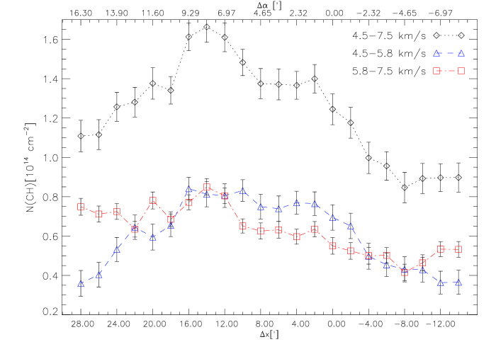
Figure 6: Column densities for $\rm{CH}$ along the observed lines of sight in TMC-1. The black diamonds represent column densities calculated from the full velocity range and the blue triangles and red squares represent column densities calculated from velocity ranges corresponding to the narrow and wide gaussian components respectively.

3.3 $\rm{H_{2}}$ column densities

The NICER method (Lombardi & Alves 2001) was applied to 2MASS data of the filament region of TMC-1 in order to acquire visual extinction values for the points overlapping with our CH observations, with the angular resolution element corresponding to the FWHM available in the radio observations. Then, by applying the $E(J-K)/N(\rm{H_{2}})=5.4\,10^{21}\ \rm{cm^{-2}mag^{-1}}$ relation from Harjunpää & Mattila (1996) and Cardelli et al. (1989), it would normally be possible to get column densities for molecular hydrogen from the extinction data alone. However, as the dense cores along the filament have high extinction values, acquiring reliable values for $A_{\rm V}$ around them by using the NICER-method alone is unreliable due to very low star densities close to and inside the cores.

As an alternative means of obtaining $\rm{H_{2}}$ column densities we used submillimetre dust continuum maps. The 850 and 450 $\mu$m SCUBA maps of the TMC-1 region from Nutter et al. (2008) were kindly provided for us by David Nutter. After convolving them to the FWHM of our 9 cm observations (228”) these were used to estimate $N$($\rm{H_{2}}$) in the positions observed in CH. The scan-mapping mode used in the SCUBA observations involves chopping by a maximum throw of 68${\rm\arcsec}$. The continuum maps are not sensitive to spatial scales larger than that. In order to compare the dust maps with the extinction and CH line data, we need to convolve the 850 and 450 mum SCUBA maps to the FWHM of 228${\rm\arcsec}$ of our 9 cm observations. We believe that in the vicinity of the TMC-1 ridge where the dust emission is likely to be dominated by compact cores this convolution results in reasonable ”smoothed” flux densities. Furthermore, we attempt to correct for the arbitrary background level of the SCUBA maps by correlating the intensities with the extinction values as desribed below. The 850 $\mu$m SCUBA maps around the Bull’s Tail smoothed to 30${\rm\arcsec}$ and 228${\rm\arcsec}$ resolutions are shown in Figs. 1a and 1b, respectively.

The H₂ column density is related to the intensity of the dust emission by

$$N({\rm H_{2}})=\frac{I_{\rm\nu}}{B_{\rm\nu}(T_{d})\cdot 2.8m_{H}\cdot\kappa_{\rm\nu}\cdot R_{d}},$$ (3)

where $B_{\rm\nu}(T_{\rm d})$ is the Planck function, $T_{\rm d}$ is the temperature of the dust, $m_{\rm H}$ is the mass of a hydrogen atom, $\kappa_{\rm\nu}$ is the dust cross-section per unit mass of dust and $R_{d}$ is the dust-to-gas ratio. For $\kappa_{\rm\nu}$ and $R_{d}$ we used the values $0.13\,{\rm cm^{2}g^{-1}}$ (at 850 $\mu$m) and 1/100, respectively.

As bolometer maps usually do, the SCUBA maps contain negative artefacts, i.e. hollows, around bright emission regions. This causes an uncertainty to the absolute level of the intensity $I_{\rm\nu}$, and suggests a need for performing a bias correction. We combined the NICER-generated extinction map with the SCUBA maps to examine the relation between extinction and submm intensity much in the same way as was done by Bianchi et al. (2003). This examination can provide us with two things: A bias correction for the SCUBA maps, and the average temperature of the dust along the filament.

A linear fit of the form

$$I^{\rm{obs}}_{\rm\nu}=\delta_{\rm\nu}+\gamma_{\rm\nu}A_{\rm V}.$$ (4)

was performed to the pixel by pixel correlations between the observed intensities at 850 or 450 $\mu$m and the visual extinction. The fit was done using pixels with $A_{\rm V}<12$, because above this level the extinctions are highly uncertain (see above), and because the dust temperature, $T_{\rm d}$, is expected to decrease towards the most obscure regions, causing a curvature in the correlation (see Bianchi et al. 2003).

The coefficient $\delta_{\rm\nu}$ should be zero in a properly biased map. The intensity of the dust emission is given by

$$I^{\rm{dust}}_{\rm\nu}=B_{\rm\nu}(T_{\rm d})(1-e^{-\tau_{\rm\nu}})\approx B_{\rm\nu}(T_{\rm d})\tau_{\rm\nu}\;,$$ (5)

where the optical thickness, $\tau_{\rm\nu}$, of the source of emission can be written as $\tau_{\rm\nu}=\Sigma\kappa_{\rm\nu}R_{\rm d}$, where $\Sigma$ is the surface density of the cloud. It can be assumed that subtracting the fitting parameter $\delta_{\rm\nu}$ from the 850 and 450 $\mu$m intensity maps should result in a better-than-nothing correction to the bias.

The dust temperature was obtained from the ratio of the $\gamma$ coefficients at the two frequencies:

$$\frac{\gamma_{\rm\nu 1}}{\gamma_{\rm\nu 2}}=\frac{\kappa_{\rm\nu 1}}{\kappa_{\rm\nu 2}}\frac{B_{\rm\nu 1}(T_{d})}{B_{\rm\nu 2}(T_{d})}=\left(\frac{\nu_{1}}{\nu_{2}}\right)^{\beta}\frac{B_{\rm\nu 1}(T_{d})}{B_{\rm\nu 2}(T_{d})}\;.$$ (6)

In the latter form, we have made use of the assumption that at (sub)millimetre wavelengths $\kappa_{\rm\nu}\propto\nu^{\beta}$, where the emissivity index $\beta=1.95$ between 850 and 450 $\mu$m (Ossenkopf & Henning 1994).

As the dust temperature, and possibly also the ratio dust opacities in the submm and in the visual, $\kappa_{\rm\nu}/\kappa_{\rm V}$, can be expected to be different in the filament when compared to several other parts of the cloud, the examination of the linear relation between observed intensities and extinctions were done only on pixels in a rectangular area passing along the filament with a width of about $400\arcsec$. Linear fits were performed in these areas for comparing both the $450\ \rm{\mu m}$ and $850\ \rm{\mu m}$ maps to the visual extinctions as calculated with the NICER method. These comparisons and the linear fits performed on them are presented in Figs. 7a and 7b. With the help of these fits we corrected the bias on the intensity maps, and calculated the average dust temperature of the examined area to be $T_{d}=(11.0\pm 2.7)\ \rm{K}$. After this, with the help of Eq. 3, it was possible to use the $850\ \rm{\mu m}$ (because it seemed more accurate) SCUBA map to calculate the $\rm{H_{2}}$ column densities on the points overlapping with our $\rm{CH}$ observations (three points in the southeast were not covered by the SCUBA maps). The resulting $N(\rm{H_{2}})$ estimates are plotted in Fig. 8 as a dashed line.

The column densities calculated in this fashion agree rather well with those estimated from the $A_{\rm V}$ map on the northwestern side of the map ($\Delta x\leq 0^{\prime}$, see Fig. 8), whereas the agreement is not good in the southeast. However, it is conceivable that the $A_{\rm V}$ map reflects the true H₂ column density distribution except for the regions of the highest obscuration, in particular it should do so at both ends of the strip observed in CH.

The discrepancy between the $N({\rm H_{2}})$ estimates from the 850 $\mu$m emission presented above and those from $A_{\rm V}$ can be caused by the fact that assumption of a constant dust temperature is not valid. We examined therefore the possible variations of the dust temperature along the filament by using the ’bias-corrected’ 450 $\mu$m and 850 $\mu$m intensities in the formula

$$\frac{I^{*}_{\rm\nu_{2}}}{I^{*}_{\rm\nu_{1}}}\left(\frac{\nu_{1}}{\nu_{2}}\right)^{3.0+\beta}=\frac{e^{h\nu_{1}/kT_{d}}-1}{e^{h\nu_{2}/kT_{d}}-1}.$$ (7)

This method can be applied with a reasonable accuracy to the positions within the dense filament where both 450 and 850 $\mu$m signals are strong. The resulting dust temperatures and H₂ column densities are presented in Table 1 and as a dotted line in Fig. 8. It is worth noting that the that, in the envelope, the dust temperature calculated in this fashion is similar to the $T_{\rm d}=12\ {\rm K}$ derived by Nutter et al. for the shoulder component. This is also quite close to kinetic gas temperatures observed in the cloud by e.g. Pratap et al. (1997).

Since the extinction method seems reliable everywhere except at three points ($\Delta x=2\arcmin\ldots 6\arcmin$) around the calculated extinction value maximum and because the dust temperature seems to be variable along the filament, we have opted to use the extinction-derived $N({\rm H_{2}})$ values for all except the three aforementioned points. For these three points we use instead the $N({\rm H_{2}})$ values calculated by using dust temperatures acquired from Eq. 7. These column densities are listed in the sixth column of Table 1.

(a)

(b)

Figure 7: A linear fit to the visual extinctions and (a) $850\ \rm{\mu m}$ or (b) $450\ \rm{\mu m}$ intensities around the filament region of TMC-1. The resolution of the intensities and the extinctions both correspond to a beam FWHM of $228\arcsec$.

Figure 8: Column densities for $\rm{H_{2}}$ along the TMC-1 filament. The dashed line represents molecular hydrogen column densities calculated with Eq. 3 while assuming a constant dust temperature of $T_{d}\approx 11.0\ \rm{K}$. The diamonds represent $N$($\rm{H_{2}}$) values derived from a NICER extinction map as described in the beginning of section 3.3. The triangles and the dotted line represent $N$(H₂) values calculated by using variable dust temperatures obtained from Eq. 7.

3.4 CH abundance

When comparing the column densities of $\rm{H_{2}}$ and $\rm{CH}$ in an x,y-plot, the slope of a linear fit performed on the data points should tell the average abundance of CH in the observed area. This approach is however not very interesting if the two column densities do not correlate very well. No strong correlation ($\rho\approx 0.53$) between the two column densities was noticed, suggesting that the fractional abundance of CH is not very constant throughout the region. The abundance of CH, or $X({\rm CH})=N({\rm CH})/N({\rm H_{2}})$, along the observed axis is presented in Fig. 9. This figure shows, beginning from $\Delta x=+8\arcmin$, a steady rise in $X(\rm{CH})$ from about $1.0\,10^{-8}$ up to $\sim 2.2\,10^{-8}$ towards the southeastern end of the filament. Our result at the cyanopolyyne peak matches the value quoted in Ohishi et al. (1992). Examining the abundance of CH calculated by using $N$(CH) from the narrow and wide line components is not very useful because we can not evaluate $N$(H₂) from the two different velocity intervals separately and thus we refrained from doing so.

Figure 9: The abundances of CH and OH along the observed lines of sight in TMC-1.

3.5 Correlation with $\rm{OH}$

We had access to previous OH spectral line data acquired by Harju et al. (2000) with partially overlapping points to our CH observations and used the formula from the same paper to acquire the column densities for OH:

$$N({\rm OH})=4.04\,10^{14}\frac{1}{1-T_{\rm bg}/T_{\rm ex}}\cdot\frac{1}{\eta_{\rm C}}\int T_{\rm MB}(1665)dv$$ (8)

with $[\rm{Kkms^{-1}}]$ as the unit for the line area and $[\rm{cm^{-2}}]$ as the unit for the resulting column density. The excitation temperature and main beam efficiency used for this was $T_{\rm{ex}}=10\ \rm{K}$ and $\eta_{\rm{C}}=30\ \%$. The velocity interval ($4.5\ \rm{km/s}\ldots 6.5\ \rm{km/s}$) of the integrated line area was chosen to be identical to the one used for the CH column density calculations. The resulting column densities are listed in the fifth column of Table 1 and they are plotted in Fig. 10.

Figure 10: Column densities for $\rm{OH}$ and CH along the TMC-1 filament. The arrows point out the approximate location of the cyanopolyyne maximum as per Olano et al. (1988).

As can be seen from Table 1, there are twice as many CH observations as there are OH observations along the strip we are investigating. To make use of all the CH observations when comparing them to OH, we have used a simple but sufficient averaging scheme where, on each overlapping CH and OH observation, we take a weighted average of CH and its adjacent point on each side and give the adjacent points a weight of one half. The overlapping observations are plotted to Fig. 11 along with a linear fit made between the points. A strong correlation ($R_{\rm{CH,OH}}\approx 0.90$) is noticed between the column densities and the column densities follow the relation

$$N({\rm OH})[{\rm cm^{-2}}]=(11.2\pm 2.1)\,10^{14}+(10.1\pm 1.6)\cdot N({\rm CH})\;.$$ (9)

The fractional abundance of OH along the TMC-1 ridge is plotted together with that of CH in Fig. 9. As the CH column density lies in the range $\sim 0.9-1.6\,10^{14}$ cm^-2 the derived OH/CH abundance ratio along the ridge, $N$(OH)/$N$(CH)$\sim 16-20$, is clearly larger than that measured recently in diffuse interstellar gas by Weselak et al. (2009): $N$(OH)/$N$(CH)$\sim 2.6$, which is close to the atomic O/C ratio in the local ISM (e.g. Duley & Williams 1984; Wilson & Rood 1994).

Figure 11: Correlation plot of the column densities of CH versus OH in spots where observations of them overlap.

4 Discussion

4.1 The chemistry of CH and its relation to OH

Pure gas-phase chemistry models (e.g. Viala 1986) predict that the CH abundance, $X({\rm CH})$, decreases from $\sim 10^{-8}$ at the outer boundaries of molecular clouds ($A_{\rm V}\leq 1$) to $<10^{-9}$ towards the cloud interiors. This change should imply saturation in the correlation of $N({\rm CH})$ with $N({\rm H_{2}})$ towards dense molecular clouds, and indeed this kind of tendency can be traced in observational results (Hjalmarson et al. 1977; Mattila 1986; Qin et al. 2010).

The production of CH depends on the availability of C⁺ or C. C⁺ is the dominant form of carbon in the outer parts of a cloud exposed to UV radiation. In the inner parts, C⁺ formation is hindered by the lack of UV photons and if formed is rapidly neutralized or incorporated into neutral molecular species via ion-molecule and dissociative recombination reactions. When the elemental O/C ratio is larger than unity, most carbon is consumed by the formation of gas-phase CO, which eventually freezes onto grain surfaces at sufficiently low temperatures, $\lesssim$ 20 K.

The principal source of CH in dark clouds is likely to be the dissociative recombination of hydrocarbon ions, in particular CH${}_{3}^{+}$ and CH${}_{5}^{+}$, e.g.:

$${\rm CH}_{3}^{+}+e^{-}\rightarrow{\rm CH}+{\rm H_{2}}\;.$$ (10)

The sequence leading to these ions is initiated either by the radiative association of C⁺ and H₂:

$${\rm C}^{+}+{\rm H_{2}}\rightarrow{\rm CH_{2}^{+}}+h\nu\;,$$ (11)

or by the proton exchange reaction between neutral C and H${}_{3}^{+}$:

$${\rm C}+{\rm H_{3}^{+}}\rightarrow{\rm CH^{+}}+{\rm H_{2}}$$ (12)

(e.g. Black et al. 1975, and references therein). The sequence continues to larger hydrocarbon ions through reactions with H₂. CH is thus expected to correlate with C⁺ and C I, and because these species are necessary to the production of complex carbon compounds, it should correlate also with heavier hydrocarbons and cyanopolyynes. Furthermore, a close relationship between CH and long carbon chains or cyclic molecules may originate in direct CH insertion into an unsaturated hydrocarbon (followed by H elimination) which is likely to proceed with a small or no barrier (e.g. Soorkia et al. 2010, and references therein).

The destruction of CH is thought to occur primarily via the following neutral exchange reactions:

$$\begin{array}[]{ccc}{\rm CH}+{\rm O}&\rightarrow&{\rm CO}+{\rm H}\\ {\rm CH}+{\rm N}&\rightarrow&{\rm CN}+{\rm H}\;.\end{array}$$ (13)

In contrast with pure gas-phase chemistry, models including accretion of molecules onto grain surfaces predict a smooth distribution for the CH abundance in dense clouds. Hartquist & Williams (1989) and Rawlings et al. (1992) have pointed out that the CH abundance may remain almost unchanged in the dense interiors of dark clouds where heavy molecules are likely to be depleted. As long as some gas-phase CO is available, carbon ions are supplied by reaction with He⁺ (which is continually produced by cosmic rays):

$${\rm He^{+}}+{\rm CO}\rightarrow{\rm C^{+}}+{\rm O}+{\rm He}\;.$$ (14)

The reduction of CO is partly compensated by the diminishing destruction of CH by O or N. Also an increase in the H${}_{3}^{+}$ abundance associated with the depletion can have a balancing effect on the CH abundance. Furthermore, the adsorption energy of CH is relatively low and it is efficiently returned to the gas-phase via thermal desorption (Aikawa et al. 1997).

In dark clouds, the reactions leading to the formation and destruction of OH are probably analogous to those for CH. It is thus expected that OH is mainly produced by dissociative recombination of H₃O⁺ and destroyed in neutral exchange reactions with C, N, and O atoms. In order to identify the most important reactions and to study temporal changes in the OH/CH abundance ratio, we ran some chemical models which, although relatively simple, are appropriate for dark clouds such as TMC-1.

We modeled the chemistry of TMC-1 by treating the source as a homogeneous, isotropic cloud with the constant physical parameters, $n({\rm H_{2}})=10^{4}\,{\rm cm}^{-3}$, $T=10$ K (for both gas and dust) and $A_{\rm V}=10$ mag, $\sigma_{\rm g}\approx 0.03\ \rm{\mu m}$, using a cosmic-ray ionisation rate of $1.3\,10^{-17}\,{\rm s}^{-1}$ and performing a pseudo-time-dependent calculation in which the chemistry evolves from initial abundances that are atomic, excepting molecular hydrogen. We adopt the low-metallicity oxygen-rich elemental abundances from Graedel et al. (1982) and Lee et al. (1998) as listed in Table 8 of Woodall et al. (2007). Thus, our initial elemental abundances with respect to H nuclei number density for C and O are $7.3\,10^{-5}$ and $1.76\,10^{-4}$, respectively, giving a C/O ratio of   0.4. Note, under dark cloud conditions, hydrogen exists primarily in molecular form so that the H nuclei number density is twice that of molecular hydrogen. Our gas-phase chemical network is the latest release of the UMIST Database for Astrochemistry or “Rate06” (http://www.udfa.net) as described in Woodall et al. (2007). We ran one model using gas-phase chemistry only and another allowing for gas-grain interactions, namely, the accretion of gas-phase species onto dust grains and the thermal desorption of species from the grain surfaces. For our second model, we assume the dust grains are spherical particles with a radius of $10^{-5}$ cm and that the dust is well mixed with the gas possessing a constant fractional abundance of $2.2\,10^{-12}$ with respect to H nuclei density. Our accretion and thermal desorption rates were calculated according to the theory outlined in Hasegawa et al. (1992), assuming a sticking coefficient of unity.

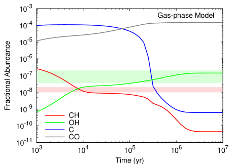
(a)

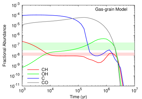
(b)

Figure 12: Plots showing the fractional abundances (with respect to H₂ number density) of CH and OH as functions of time, calculated using a gas-phase chemistry only model (a) and a gas-grain model (b) for a TMC-1-like cloud (see Sect. 4.1). Also shown in this Figure are the fractional C and CO abundances. The shaded regions represent the observed range of CH and OH fractional abundances derived by us along the TMC-1 ridge.

The fractional abundances (with respect to H₂ number density) of CH and OH are plotted in Figs. 12a and 12b as functions of time as predicted by the pure gas-phase (solid lines) and gas-grain (dot-dashed line) models. We see that the two models agree rather well until an age of approximately $2\,10^{5}$ years when the freeze out of molecules starts to take effect. In both models, the CH and OH fractional abundances show an anticorrelation until a time of about $5\,10^{5}$ years, with CH continually declining and OH continually increasing. The OH abundance exceeds that of CH at an early time before $10^{4}$ years and remains thus for the duration of the simulation, except until very late stages in the gas-grain model. CO passes C in abundance in these models around $6-7\,10^{4}$ years.

Soon after $10^{4}$ years CH and OH plateau temporarily (until $\sim 2\,10^{5}$ year). The relative constancy of the OH/CH abundance in this time interval can be explained by very similar gas-phase production and destruction mechanisms.

According to the present model, the dissociative recombination of $\rm{H_{3}O^{+}}$ is responsible for 81 % of the OH production at a cloud age of $10^{4}$ years and for 89 % at $10^{5}$ years. It is only at the relatively young cloud age of $10^{3}$ years that dissociative recombination contributes less than 20 %. At this stage, the model predicts the reaction

$${\rm O}+{\rm HCO}\rightarrow{\rm CO}+{\rm OH}$$ (15)

to be a major process, making up 76 % of OH formation. Likewise, the dissociative recombination of $\rm{CH_{3}^{+}}$ is accountable for 72 % of CH production at $10^{4}$ years and for 69 % at $10^{3}$ years, yet contributes only 23 % at $10^{5}$ years. The main production pathway at this age is

$${\rm CH_{2}}+{\rm H}\rightarrow{\rm CH}+{\rm H_{2}}\;.$$ (16)

Since $\rm{CH_{2}}$ is also likely produced through dissociative recombination of $\rm{CH_{3}^{+}}$, this “detour” does not significantly change the overall picture. All these precursors are formed by successive hydrogenation of $\rm{CH^{+}}$ and $\rm{CH_{2}^{+}}$ ions that stem from reactions of $\rm{C^{+}}$ with $\rm{H_{2}}$ or C with $\rm{H_{3}^{+}}$. Also, $\rm{H_{3}O^{+}}$, the main precursor of OH, has a similar genesis through iterative hydrogenation of $\rm{OH^{+}}$ formed by protonation of O atoms by $\rm{H_{3}^{+}}$.

Furthermore, the destruction pathways of CH and OH are very similar. At a cloud age of $10^{5}$ years, reactions with C, N and O,

$${\rm OH}+{\rm C} \rightarrow {\rm CO}+{\rm H}\ (31\%)$$ (17)

$${\rm OH}+{\rm N} \rightarrow {\rm NO}+{\rm H}\ (19\%)$$ (18)

$${\rm OH}+{\rm O} \rightarrow {\rm O_{2}}+{\rm H}\ (49\%)$$ (19)

are exclusively destroying OH (the figures in brackets denote the relative importance of each reaction). CH is consumed by the following analogous processes:

$${\rm CH}+{\rm C} \rightarrow {\rm C_{2}}+{\rm H}\ (14\%)$$ (20)

$${\rm CH}+{\rm N} \rightarrow {\rm CN}+{\rm H}\ (21\%)$$ (21)

$${\rm CH}+{\rm O} \rightarrow {\rm CO}+{\rm H}\ (60\%)$$ (22)

A small proportion is, interestingly, due to the associative ionization (reverse dissociative recombination) of CH with O

$${\rm CH}+{\rm O}\rightarrow{\rm HCO^{+}}+{\rm e^{-}}$$ (23)

which is almost thermoneutral (although if one calculates the Gibbs energies (Hamberg et al. 2010), it becomes endoergic and probably should be removed from the model). At earlier stages (approximately $10^{3}$ years), reactions with $\rm{C^{+}}$,

$${\rm C^{+}}+{\rm CH} \rightarrow {\rm C_{2}^{+}}+{\rm H}\ (42\%)$$ (24)

$${\rm C^{+}}+{\rm CH} \rightarrow {\rm CH^{+}}+{\rm C}\ (42\%)$$ (25)

are more important, because of the higher abundances of $\rm{C^{+}}$ at this time.

The pure gas-phase and gas-grain models start showing large deviations from each other at times later than $10^{5}$ years. The fractional abundance of CH declines quickly as C is converted into CO, and in the pure gas-phase model it diminishes continually until a steady-state fractional abundance of $\approx 3\,10^{-11}$ is reached at a time of about $2\,10^{6}$ years. In the gas-grain model around a time of $10^{6}$ years, the revival of OH and CH is due to the depletion of atomic species (C, N and O) as their abundance drops rapidly after a time of about $5\,10^{5}$ years thus limiting their effectiveness at destroying the radicals. Beyond $10^{6}$ years, stable species (e.g. CO, N₂, O₂ and H₂O) become locked onto the grain surfaces thus depleting the gas-phase of all atoms and molecules. In the present model, which includes thermal desorption from grains only, both CH and OH abundances decrease rapidly after about $2\,10^{6}$ years. This behaviour is different from models which include non-thermal desorption mechanisms (cosmic ray heating, surface photodissociation, exothermic surface reactions; e.g. Garrod et al. (2007)) which predict detectable amounts of CH and OH at later times.

4.2 Distributions of CH and OH in TMC-1

When looking at our data we see in Fig. 6 a clear peak in the CH column density in the vicinity of the cyanopolyyne maximum of TMC-1, about $3\arcmin$ on its southeastern side (offset $\Delta x=+14\arcmin$). The bump in $N({\rm CH})$ begins at the offset $\Delta x=+8\arcmin$ which corresponds to the point where our strip enters the region of greatest intensity on the smoothed SCUBA map (Fig. 1b), and ends at $\Delta x=+18\arcmin$ where we exit the brightest parts.

The diagram in Fig. 6 shows also CH column densities in two velocity windows, and it is evident that the gas in the velocity range $5.8-7.5$ km s^-1 is mainly responsible for the peak. Most molecular lines observed towards this source, including those of complex carbon compounds, originate in this velocity range (e.g. Pratap et al. 1997), and it seems likely that the local CH and cyanopolyyne peaks are also nearly spatially coincident. Besides the peak at $\Delta x=+14\arcmin$ the $N({\rm CH})$ in the $V_{\rm LSR}$ range $5.8-7.5$ km s^-1 shows a tendency to increase slightly from northwest to southeast, all the way until the end of the strip where the dust column density and $N({\rm CH})$ in the low-velocity range, $4.5-5.8$ km s^-1 have decreased.

With respect to the fractional CH abundance, $X({\rm CH})$, the CP peak is not special. From Fig. 9 we see that $X({\rm CH})$ lies somewhere around $1.0\,10^{-8}$ in the northwestern part of the filament until the offset $\Delta x=+8\arcmin$, and reaches values of $\sim 2.0\,10^{-8}$ towards the southeastern end. This is the only major trend in the variation of $X({\rm CH})$ and it does not seem to vary in e.g. the vicinity of the high-extinction cores.

It is evident from Figures 9-11 that the CH abundance is well correlated with that of OH. The fractional OH abundance increases from about $2.5\,10^{-7}$ in the northwest to about $5.0\,10^{-7}$ in the southeast. Acccording to the chemical models discussed in the previous Section, a good correlation between OH and CH is expected at youthful cloud ages around $10^{4}-10^{5}$ years because of the very similar gas-phase production and destruction mechanisms. During this period, the OH/CH abundance ratio in the models increases from about 3 to about 10. It may be possible to reproduce the observed OH/CH ratio by adjusting the elemental O/C ratio and/or the physical parameters of the model. We note that during the model ages between $10^{4}$ and $10^{5}$ years the fractional C and CO abundances are within one order of magnitude from each other, which roughly agrees with the estimates of Schilke et al. (1995) and Maezawa et al. (1999).

On the other hand, the gas-grain model predictions reproduce the observed large abundances of CH and OH at later times, around 10⁶ years. Furthermore, the gas-grain model can qualitatively explain the observed spatial variations of the CH and OH abundances along the TMC-1 filament if they are interpreted in terms of evolution with the chemical age advancing from the southeast to the northwest. After the peak in OH in the gas-grain model ($\sim 1.5-2\,10^{6}$ years), both CH and OH fractional abundances decrease with increasing age, and it is only at this point in the present calculations that this particular trend is seen. Running models including a more comprehensive treatment of desorption may shift this period but most likely it would still be associated with an advanced stage where accretion onto grain surfaces plays a dominant role.

In view of the rather coarse angular resolution available in the present observations, and the fact that both CH and OH are known to have large abundances in diffuse gas, it is, however, unlikely that observed abundance gradients predominantly reflect conditions in depleted cores, which occupy a relatively small fraction of the gas encompassed by the telescope beam. A more probable explanation is that when moving from the northwestern end of the filament to the southeast we see an increasingly thick layer of tenuous gas, which would also agree with the increasing abundance of neutral carbon towards southeast suggested by the C I map of Maezawa et al. (1999). This explanation is furthermore supported by our chemical models where, if we decrease the gas density, we can see the abundances of both CH and OH increase. In this situation the density dependence overcomes the temporal anticorrelation. This tendency is probably due to an enhanced production by dissociative recombination resulting from the higher fractional abundance of electrons in low-density gas.

Hirahara et al. (1992) and Pratap et al. (1997) estimated by modelling the excitation of molecular lines that the gas volume density is somewhat higher near the ammonia peak in the northwestern part of the TMC-1 filament as compared with the CP peak. The SCUBA maps of Nutter et al. (2008) , reproduced in the present work, show that the CP peak lies in the area where the dust and gas column density reaches its maximum. This separation of volume and column density peaks implies that the southeastern part of the filament possesses a more extensive envelope of low-density gas than the northwestern part, and is readily an indication that the stages of dynamical evolution are different at the two ends of the filament.

The large abundances of CH combined with the presence of the SCUBA dust intensity maximum in the southeastern parts is consistent with the presence of the low-density envolope. The fractional abundance reached at the southeastern end of the strip, $X({\rm CH})\sim 2.0\,10^{-8}$, is slightly below half when compared to abundances observed in diffuse clouds (Liszt & Lucas 2002, e.g. $X(\rm{CH})\approx 4.3\,10^{-8}$ in $\zeta$ Per). On the other hand, the relatively constant abundance $\sim 1.0\,10^{-8}$ at the offsets $\Delta x<+8\arcmin$ is likely to correspond to the steady-state value in a dense core (averaged over a $4\arcmin$ beam). It is, however, somewhat higher than the abundances predicted by the chemistry model of Ruffle et al. (1997) where the interaction with grains is included. Then again comparing our calculated abundances to the model presented by Flower et al. (1994), we see that our abundances are slightly lower than the values presented in the model results where the depletion of oxygen $\delta_{\rm O}=1$ for a cloud with high visual optical depth. Our results would most likely match Flower’s model if a slightly higher oxygen depletion factor is used as a model where $\delta_{\rm O}=10$ produces much lower abundances than our measurements.

4.3 The structure of the filament in the light of the SCUBA map

In addition to providing us with an estimate of the hydrogen column density in TMC-1, the SCUBA maps can be analyzed from the perspective of examining the physical dimensions of the clumpy structures seen in them. That is what we intend to do in this subsection.

The clumpfind algorithm (Williams et al. 1994) was used to identify clumps, i.e. relatively isolated density enhancements, in the 850 $\rm{\mu m}$ SCUBA map of the filament from Nutter et al. (2008), smoothed to correspond to a $30\arcsec$ beam. The filament shows rather small intensity variations. The best agreement with the visual inspection is obtained by setting the intensity threshold to 0.15 Jy/beam (twice the value of the rms noise in the neighbourhood of TMC-1) and the stepsize to 0.075 Jy/beam ($1\sigma$). With this setting the algorithm finds five clumps in the filament; the properties of these clumps are listed in Table 2. The closest correspondence with the “Hirahara cores” from Hirahara et al. (1992) is also indicated. The intensity stepsize used here is half the value recommended by Williams et al. (1994). If a $2\sigma$ step is used, the program identifies 3 clumps correponding to the Hirahara cores A+B, C+D, and E (extending to the SE tip). The FWHM sizes of the clumps in $x$ and $y$ directions and the aspect ratios are calculated in a coordinate system tilted by $53.6\degr$ with respect to the R.A. axis

Table 2: Properties and closest correspondence with Hirahara cores of the four clumps found using the clumpfind algorithm on the 850 $\rm{\mu m}$ SCUBA intensity map (smoothed to $30\arcsec$ resolution).

Hirahara	Mass $[M_{\odot}]$	FWHM $X\times Y$ $[\arcmin]$	X:Y	$\Sigma$ [$\rm{g/cm^{2}}$]
A+B	3.9	$4.2\times 1.5$	2.8	0.042
C	4.2	$3.6\times 1.4$	2.6	0.045
D	3.4	$2.3\times 1.8$	1.3	0.045
E	5.3	$3.9\times 1.9$	2.0	0.041
SE tip	1.5	$2.9\times 1.4$	2.2	0.032

The total mass of the filament is 18.3 $M_{\odot}$, and the average surface density is $<\Sigma>=0.042$ g  cm^-2. Here we have assumed a constant dust temperature $T_{\rm d}$=10 K. The previous determinations of the the gas kinetic temperatures towards various positions in the cloud, including the CP and NH₃ peaks, lie invariably in the vicinity of 10 K (e.g. Pratap et al. 1997), and we think this value represents well the dust clumps seen at a $30\arcsec$ resolution. The somewhat higher temperatures derived in Sect. 3.3. by comparison between the SCUBA 450/850 maps and A_V, relate to a $228\arcsec$ beam which encompasses also core envelopes. The clumps can also be identified as five intensity maxima in Fig. 1a.

Even though the locations of the Hirahara cores are always in the vicinity of a clump on the filament, the actual peaks of the clumps and the CCS line intensities do not overlap; both of the 850 micron intensity peaks corresponding closest to cores C and D are shifted about $2\arcmin$ towards each other in relation to the CCS intensity maxima closest to the two cores. These spatial offsets are larger than the FWHM of the CCS observations.

Applying the formula quoted by Hartmann (2002) for a filament with a critical line density, one finds that the average surface density $0.042$ g  cm^-2 implies a Jeans length of $\sim 0.16$ pc or $4\arcmin$ at a distance of 140 pc. The corresponding mass is 2.7 $M_{\odot}$. The long-axes of the clumps and the avarage separations between their centres of mass ($\sim 4.8\arcmin$) are comparabable to the derived Jeans length. This suggests that the clumps identified here are formed as a result of thermo-gravitational fragmentation. The full resolution SCUBA maps and the previous high-angular resolution molecular line maps of Langer et al. (1995) suggest that the fragmentation has proceeded to still smaller structures, so that each clump is likely to contain several dense cores.

Finally, we note the overall structure of TMC-1 does not resemble the model presented in Hanawa et al. (1994), where the fragmentation of the filament is supposed to have started from one end (from the northwestern tip in this case). On the SCUBA map we see a roughly symmetrical structure, the apparent centre lying between cores C and D. The structure bears resemblance to the final density profiles resulting from the simulations of Bastien et al. (1991) for the gravitational instability in an elongated isothermal cylinder.

5 Conclusions

We report on the detection of a CH abundance gradient in TMC-1 with X(CH) increasing from $\sim 1.0\,10^{-8}$ in the northwestern end of the filament to $\sim 2.0\,10^{-8}$ in the southeastern end. The CH column density maximum lies close to cyanopolyyne (CP) peak in the southeastern part of the filament. As it belongs to the most simple carbon compounds, CH is likely to reflect the distributions of C I or C⁺. Using previously published OH observations, we also show that the fractional abundance of OH increases strongly from the northwest to the southeast. The OH/CH abundance ratio lies in the range $\sim 16-20$.

In the northwest, the CH abundance stays remarkably constant at around $1.0\,10^{-8}$. The value is clearly higher than the steady-state values predicted for dense cores by pure gas-phase chemistry models, but the agreement is better with models including gas-grain interaction. We performed calculations using the UMIST Database for Astrochemistry reaction network and a homogenous physical model appropriate for sources such as the TMC-1 ridge. The best agreement with observations for the pure gas-phase model was found at cloud ages of several $10^{5}$ years, but the predicted CH and OH fractional abundances are a factor of 3-5 lower than the observed values. Agreement is better with a gas-grain model at this age. The latter model reproduces the observed abundances at late stages where molecular depletion is significant. However, in view of the large beam used in the observations, and the likely encompassment of low-density gas, it is doubtful that the derived abundances reflect conditions in depleted cores.

The dust continuum map from SCUBA (Nutter et al. 2008, smoothed to the $\leavevmode\nobreak\ 4\arcmin$ resolution of the CH observations) suggests that in the vicinity of the CP peak the filament has an extensive envelope, in contrast to the neighbourhood of the NH₃ peak which appears to be more compressed. As the CH and OH abundances are expected to be anticorrelated with density, their larger abundances in the southeast are likely to be due to this low-density envelope. The largest fractional CH and OH abundances are found at the southeastern end of TMC-1 where we are approaching the ”C I peak” discovered by Maezawa et al. (1999).

The total H₂ column density distribution along the TMC-1 filament was calculated by combining the SCUBA 850 and 450 $\mu$m maps with an $A_{\rm V}$ map from 2MASS data. The distribution peaks between the CP and NH₃ maxima. In fact, the high-resolution SCUBA map at 850 $\mu$m shows a rather symmetric structure with the apparent centre between the Hirahara cores C and D. The sizes and typical separations of clumps correspond to the Jeans’ length in an isothermal filament with the observed surface density. The main difference between the two ends of the filament seems to be the presence of the low-density envelope in the southeast, which probably is an indication of an early stage of dynamical evolution. As lower densities result in slower reaction rates, this finding conforms with the suggestion of several previous studies that the southeastern end of the cloud is also chemically less evolved than the northeastern end.