Phase Transitions in Soft Matter Induced by Selective Solvation

Abstract

We review our recent studies on selective solvation effects in phase separation in polar binary mixtures with a small amount of solutes. Such hydrophilic or hydrophobic particles are preferentially attracted to one of the solvent components. We discuss the role of antagonistic salt composed of hydrophilic and hydrophobic ions, which undergo microphase separation at water-oil interfaces leading to mesophases. We then discuss phase separation induced by a strong selective solvent above a critical solute density $n_{\rm p}$, which occurs far from the solvent coexistence curve. We also give theories of ionic surfactant systems and weakly ionized polyelectrolytes including solvation among charged particles and polar molecules. We point out that the Gibbs formula for the surface tension needs to include an electrostatic contribution in the presence of an electric double layer.

I Introduction

In soft matter physics, much attention has been paid to the consequences of the Coulombic interaction among charged objects, such as small ions, charged colloids, charged gels, and polyelectrolytes Levin ; Barrat ; Holm ; Rubinstein ; PG ; Safran . However, not enough effort has been made on solvation effects among solutes (including hydrophobic particles) and polar solvent molecules Is ; Marcus ; Gut ; Chandler . Solvation is also called hydration for water and for aqueous mixtures. In mixtures of a water-like fluid and a less polar fluid (including polymer solutions), the solvation is preferential or selective, depending on whether the solute is hydrophilic or hydrophobic. See Fig.1 for its illustration. The typical solvation free energy much exceeds the thermal energy $k_{B}T$ per solute particle. Hence selective solvation should strongly influence phase behavior or even induce a new phase transition. In experiments on aqueous mixtures, it is well known that a small amount of salt drastically alters phase behavior polar1 ; polar3 ; Misawa ; Kumar ; cluster ; Taka ; Anisimov . In biology, preferential interactions between water and cosolvents with proteins are of crutial importance Tima ; Tima1 . Thus selective solvation is relevant in diverse fields, but its understanding from physics is still in its infancy.

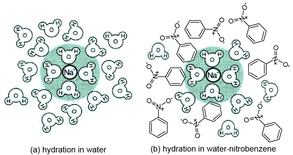
Figure 1: Illustration of hydration of Na⁺ surrounded by a shell composed of water molecules in (a) pure water and (b) water-nitrobenzene. The solvation chemical potential of Na⁺ is higher for (b) than for (a).

Around 1980, Nabutovskii et al.R1 ; R2 proposed a possibility of mesophases in electrolytes from a coupling between the composition and the charge density in the free energy. In aqueous mixtures, such a coupling originates from the selective solvationOnukiJCP04 ; OnukiPRE . It is in many cases very strong, as suggested by data of the Gibbs transfer free energy in electrochemistry (see Sec.2). Recently, several theoretical groups have proposed Ginzburg-Landau theories on the solvation in mixture solvents for electrolytes OnukiJCP04 ; OnukiPRE ; OnukiJCP ; Tsori ; Ro1 ; Ro2 ; An1 ; Araki ; Nara ; Daan ; Okamoto , polyelectrolytesOnuki-Okamoto ; Oka , and ionic surfactants OnukiEPL . In soft matter physics, such coarse-grained approaches have been used to understand cooperative effects on mesoscopic scales PG ; Safran ; Onukibook , though they are inaccurate on the angstrom scale. They are even more usuful when selective solvation comes into play in the strong coupling limit. This review presents such examples found in our recent research.

1.1 Antagonistic salt. An antagonistic salt consists of hydrophilic and hydrophobic ions. An example is sodium tetraphenylborate NaBPh₄, which dissociates into hydrophilic Na⁺ and hydrophobic BPh${}_{4}^{-}$. The latter ion consists of four phenyl rings bonded to an ionized boron. Such ion pairs in aqueous mixtures behave antagonistically in the presence of composition heterogeneity. (i) Around a water-oil interface, they undergo microphase separation on the scale of the Debye screening length $\kappa^{-1}$, while homogeneity holds far from the interface to satisfy the charge neutrality (see the right bottom plate in Fig.2). This unique ion distribution produces a large electric double layer and a large Galvani potential difference OnukiPRE ; OnukiJCP ; Araki ; Nara . We found that this ion distribution serves to much decrease the surface tension OnukiJCP , in agreement with experiments Reid ; Luo . From x-ray reflectivity measurements, Luo et al. Luo determined such ion distributions around a water-nitrobenzene(NB) interface by adding BPh${}_{4}^{-}$ and two species of hydrophilic ions. (ii) In the vicinity of the solvent criticality, antagonistic ion pairs interact differently with water-rich and oil-rich composition fluctuations, leading to mesophases (charge density waves). In accord with this prediction, Sadakane et al. Sadakane ; Seto added a small amount of NaBPh₄ to a near-critical mixture of D₂O and 3-methylpyridine (3MP) to find a peak at an intermediate wave number $q_{m}$($\sim 0.1~{}$Å${}^{-1}\sim\kappa$) in the intensity of small-angle neutron scattering. The peak height was much enhanced with formation of periodic structures. (iii) Moreover, Sadakane et al. observed multi-lamellar (onion) structures at small volume fractions of 3MP (in D₂O-rich solvent) far from the criticality SadakanePRL , where BPh${}_{4}^{-}$ and solvating 3MP form charged lamellae. These findings demonstrate very strong hydrophobicity of BPh${}_{4}^{-}$. (iv) Another interesting phenomenon is spontaneous emulsification (formation of small water droplets) at a water-NB interface Aoki ; Poland . It was observed when a large pure water droplet was pushed into a cell containing NB and antagonistic salt (tetraalkylammonium chloride). This instability was caused by ion transport through the interface.

1.2 Precipitation due to selective solvation. Many experimental groups have detected large-scale, long-lived heterogeneities (aggregates or domains) emerging with addition of a hydrophilic salt or a hydrophobic solute in one-phase states of aqueous mixturesS1 ; S2 ; S3 ; S4 ; S5 ; S6 ; S7 . Their small diffusion constants indicate that their typical size is of order $10^{3}{\rm\AA}$ at very small volume fractions. In two-phase states, they also observed a third phase visible as a thin solid-like plate at a liquid-liquid interface in two-phase states third . In our recent theory Okamoto , for sufficiently strong solvation preference, a selective solute can induce formation of domains rich in the selected component even very far from the solvent coexistence curve. This phenomenon occurs when the volume fraction of the selected component is relatively small. If it is a majority component, its aggregation is not needed. This precipitation phenomenon should be widely observable for various combinations of solutes and mixture solvents.

1.3 Selective hydrogen bonding. Hydrogen bonding is of primary importance in the phase behavior of soft matter. In particular, using statistical-mechanical theories, the origin of closed-loop coexistence curves was ascribed to the hydrogen bonding for liquid mixtures Wheeler ; Goldstein and for polymer solutions hydrogen1 ; hydrogen2 . Interestingly, water itself can be a selective solute triggering phase separation when the hydrogen bonding differs significantly between the two components, as observed in a mixture of methanol-cyclohexane Jacobs ; Be . More drastically, even water absorbed from air changed the phase behavior in films of polystyrene(PS)- polyvinylmethylether(PVME) Hashimoto . That is, a small amount of water induces precipitation of PVME-rich domains. For block copolymers, similar precipitation of micelles can well be expected when a small amount of water is added.

1.4 Ionic surfactant. Surfactant molecules are strongly trapped at an interface due to the amphiphilic interaction even if their bulk density is very low PG-Taupin ; Safran . They can thus efficiently reduce the surface tension, giving rise to various mesoscopic structures. However, most theoretical studies have treated nonionic surfactants, while ionic surfactants are important in biology and technology. In this review, we also discuss selective solvation in systems of ionic surfactants, counterions, and added ions in water-oilOnukiEPL . We shall see that the adsorption behavior strongly depends on the selective solvation.

1.5 Polyelectrolytes. Polyelectrolytes are already very complex because of the electrostatic interaction among charged particles (ionized monomers and mobile ions) Barrat ; Holm ; Rubinstein . Furthermore, we should take into account two ingredientsOnuki-Okamoto , which have not yet attracted enough attention. First, the dissociation (or ionization) on the chains should be treated as a chemical reaction in many polyelectrolytes containing weak acidic monomers Joanny ; Bu1 ; Bu2 . Then the degree of ionization is a space-dependent annealed variable. Second, the solvation effects should come into play because the solvent molecules and the charged particles interact via ion-dipole interaction. Many polymers themselves are hydrophobic and become hydrophilic with progress of ionization in water. This is because the decrease of the free energy upon ionization is very large. It is also worth noting that the selective solvation effect can be dramatic in mixture solventsOka . As an example, precipitation of DNA has been observed with addition of ethanol in water B1 ; B2 ; B3 , where the ethanol added is excluded from condensed DNA, suggesting solvation-induced wetting of DNA by water. In polyelectrolyte solutions, macroscopic phase separation and mesophase formation can both take place, sensitively depending on many parameters.

The organization of this paper is as follows. In Sec.2, we will present the background of the solvation on the basis of some experiments. In Sec.3, we will explain a Ginzburg-Landau model for electrolytes accounting for selective solvation. In Sec.4, we will treat ionic surfactants by introducing the amphiphilic interaction together with the solvation interaction. In Sec.5, we will examine precipitation induced by a strong selective solute, where a simulation of the precipitation dynamics will also be presented. In Sec.6, we will give a Ginzburg-Landau model for weakly ionized polyelectrolytes accounting for the ionization fluctuations and the solvation interaction. In Appendix A, we will give a statistical theory of hydrophilic solvation at small water contents in oil.

II Background of selective solvation of ions

2.1 Hydrophilic ions in aqueous mixtures. Several water molecules form a solvation shell surrounding a small ion via ion-dipole interaction Is , as in Fig.1. Cluster structures produced by solvation have been observed by mass spectrometric analysis W1 ; W2 . Here we mention an experiment by Osakai et al Osakai , which demonstrated the presence of a solvation shell in a water-NB mixture in two-phase coexistence. They measured the amount of water extracted together with hydrophilic ions in a NB-rich region coexisting with a salted water-rich region. A water content of $0.168$M (the water volume fraction $\phi$ being 0.003) was already present in the NB-rich phase without ions. They estimated the average number of solvating water molecules in the NB-rich phase to be 4 for Na⁺, 6 for Li⁺, and 15 for Ca²⁺ per ion. Thus, when a hydrophilic ion moves from a water-rich region to an oil-rich region across an interface, a considerable fraction of water molecules solvating it remain attached to it. Furthermore, using proton NMR spectroscopy, Osakai et al. proton studied successive formation of complex structures of anions X^- (such as Cl^- and Br^-) and water molecules by gradually increasing the water content in NB. This hydration reaction is schematically written as X^-(H₂O)_m-1 + H₂O $\leftarrow\rightarrow$ X^-(H₂O)_m ($m=1,2,3,...$). For Br^-, these clusters are appreciable for water content larger than $0.1$M or for water volume fraction $\phi$ exceeding $0.002$.

In Appendix A, we will calculate the statistical distribution of clusters composed of ions and polar molecules. Let the free energy typically decrease by $\epsilon_{{\rm b}i}$ upon binding of a polar molecule to a hydrophilic ion of species $i$. A well-defined solvation shell is formed for $\epsilon_{{\rm b}i}\gg k_{B}T$, where the water volume fraction $\phi$ needs to satisfy

$$\phi>\phi_{{\rm sol}}^{i}\sim\exp(-\epsilon_{\rm{b}i}/k_{B}T).$$ (2.1)

For $\phi\ll\phi_{{\rm sol}}^{i}$ there is almost no solvation. The crossover volume fraction $\phi_{{\rm sol}}^{i}$ is very small for strongly hydrophilic ions with $\epsilon_{\rm{b}i}\gg k_{B}T$. For Br^- in water-NB, we estimate $\phi_{{\rm sol}}^{i}\sim 0.002$ from the experiment by Osakai et al. as discussed aboveproton .

2.2 Hydrophobic particles. Hydrophobic objects are ubiquitous in nature, which repel water because of the strong attraction among hydrogen-bonded water molecules themselves Is ; Chandler . Hydrophobic particles tend to form aggregates in water Pratt-hyd ; Wolde-Chandler and are more soluble in oil than in water. They can be either neutral or charged. A widely used hydrophobic anion is BPh${}_{4}^{-}$. In water, a large hydrophobic particle $(\gtrsim 1$nm) is even in a cavity separating the particle surface from water Chandler . In a water-oil mixture, on the other hand, hydrophobic particles should be in contact with oil molecules instead. This attraction can produce significant composition heterogeneities on mesoscopic scales around hydrophobic objects, which indeed takes place around protein surfaces Tima ; Tima1 .

2.3 Solvation chemical potential. We introduce a solvation chemical potential $\mu_{\rm sol}^{i}(\phi)$ in the dilute limit of solute species $i$. It is the solvation part of the chemical potential of one particle (see Eq.(B1) in Appendix B). It is a statistical average over the thermal fluctuations of the molecular configurations. In mixture solvents, it depends on the ambient water volume fraction $\phi$. For planar surfaces or large particles (such as proteins), we may consider the solvation free energy per unit area.

Born Born calculated the polarization energy of a polar fluid around a hydrophilic ion with charge $Z_{i}e$ using continuum electrostatics to obtain the classic formula,

$$(\mu_{\rm sol}^{i})_{\rm Born}=-({Z_{i}^{2}e^{2}}/{2R_{i}})(1-1/\varepsilon).$$ (2.2)

The contribution without polarization ($\varepsilon=1$) or in vacuum is subtracted and the $\phi$ dependence here arises from that of the dielectric constant $\varepsilon=\varepsilon(\phi)$ (see Eq.(3.5) below). The lower cutoff $R_{i}$ is called the Born radius, which is on the order of $1{\rm\AA}$ for small metallic ions Is ; RMarcus . The hydrophilic solvation is stronger for smaller ions, since it arises from the ion-dipole interaction. In this original formula, neglected are the formation of a solvation shell, the density and composition changes (electrostriction), and the nonlinear dielectric effect.

For mixture solvents, the binding free energy between a hydrophilic ion and a polar molecule is estimated from the Born formula (2.1) as $\epsilon_{\rm{b}i}\sim-\partial[(\mu_{\rm sol}^{i})_{\rm Born}]/\partial\phi$ or OnukiJCP04

$$\epsilon_{\rm{b}i}\sim Z_{i}^{2}e^{2}\varepsilon_{1}/R_{i}\varepsilon^{2}=k_{B}TZ_{i}^{2}\ell_{B}\varepsilon_{1}/R_{i}\varepsilon,$$ (2.3)

where $\varepsilon_{1}=\partial\varepsilon/\partial\phi$ and $\ell_{B}=e^{2}/k_{B}T\varepsilon$ is the Bjerrum length ($\sim 7{\rm\AA}$ for water at room temperatures). For $\varepsilon_{1}\sim\varepsilon$, a well-defined shell appears for $Z_{i}^{2}\ell_{B}\gg R_{i}$. The solvation chemical potential $\mu_{\rm sol}^{i}(\phi)$ of hydrophilic ions in water-oil should largely decrease to negative values in the narrow range $0<\phi<\phi_{\rm sol}^{i}$, as will be described in Appendix A. In the wide composition range (2.1), its composition dependence is still very strong such that $|\partial\mu_{\rm sol}^{i}/\partial\phi|\gg k_{B}T$ holds (see the next subsection). The solubility of hydrophilic ions should also increase abruptly in the narrow range $\phi<\phi_{\rm sol}^{i}$ with addition of water to oil. Therefore, solubility measurements of hydrophilic ions would be informative at very small water contents in oil.

In sharp contrast, $\mu_{\rm sol}^{i}$ of a neutral hydrophobic particle increases with increasing the particle radius $R$ in water Chandler . It is roughly proportional to the surface area $4\pi R^{2}$ for $R\gtrsim 1$nm and is estimated to be about $100k_{B}T$ at $R\sim 1$nm. In water-oil solvents, on the other hand, it is not easy to estimate the $\phi$ dependence of $\mu_{\rm sol}^{i}$. However, $\mu_{\rm sol}^{i}$ should strongly increase with increasing the water composition $\phi$, since hydrophobic particles (including ions) effectively attract oil moleculesTima1 ; SadakanePRL .

2.4 Gibbs transfer free energy. We consider a liquid-liquid interface between a polar (water-rich) phase $\alpha$ and a less polar (oil-rich) phase $\beta$ with bulk compositions $\phi_{\alpha}$ and $\phi_{\beta}$ with $\phi_{\alpha}>\phi_{\beta}$. The solvation chemical potential $\mu_{\rm sol}^{i}(\phi)$ takes different values in the two phases due to its composition dependence. So we define

$$\Delta\mu_{\alpha\beta}^{i}=\mu_{\rm sol}^{i}(\phi_{\beta})-\mu_{\rm sol}^{i}(\phi_{\alpha}).$$ (2.4)

In electrochemistry Hung ; Ham ; Koryta ; Osakai ; Sabela , the difference of the solvation free energies between two coexisting phases is called the standard Gibbs transfer free energy denoted by $\Delta G_{\alpha\beta}^{i}$ for each ion species $i$. Since it is usually measured in units of kJ per mole, its division by the Avogadro number $N_{A}$ gives our $\Delta\mu_{\alpha\beta}^{i}$ or $\Delta\mu_{\alpha\beta}^{i}=\Delta G_{\alpha\beta}^{i}/N_{A}$. With $\alpha$ being the water-rich phase, $\Delta\mu_{\alpha\beta}^{i}$ is positive for hydrophilic ions and is negative for hydrophobic ions from its definition (2.4). See Appendix B for relations between $\Delta\mu_{\alpha\beta}^{i}$ and other interface quantities.

For ions, most data of $\Delta G_{\alpha\beta}^{i}$ are at present limited on water-NB Hung ; Koryta ; Osakai and water-1,2-dichloroethane(EDC) Sabela at room temperatures, where the dielectric constant of NB ($\sim 35$) is larger than that of EDC ($\sim 10$). They then yield the ratio $\Delta\mu_{\alpha\beta}^{i}/k_{B}T$. In the case of water-NB, it is $13.6$ for Na⁺, $27.1$ for Ca²⁺, and $11.3$ for Br^- as examples of hydrophilic ions, while it is $-14.4$ for hydrophobic BPh${}_{4}^{-}$. In the case of water-EDC, it is $22,7$ for Na⁺ and $17.5$ for Br^-, while it is $-14.1$ for BPh${}_{4}^{-}$. The amplitude $|\Delta\mu_{\alpha\beta}^{i}|/k_{B}T$ for hydrophilic ions is larger for EDC than for NB and is very large for multivalent ions. Interestingly, $\Delta\mu_{\alpha\beta}^{i}$ for H⁺ (more precisely hydronium ions H₃O⁺) assumes positive values close to those for Na⁺ in these two mixtures.

In these experiments on ions, a hydration shell should have been formed around hydrophilic ions even in the water-poor phase $\beta$ (presumably not completelyproton ). From Eq.(2.1) $\phi_{\beta}$ should be exceeding the crossover volume fraction $\phi_{\rm{sol}}^{i}$. The data of the Gibbs transfer free energy quantitatively demonstrate very strong selective solvation even in the range (2.1) or after the shell formation.

On the other hand, neutral hydrophobic particles are less soluble in a water-rich phase $\alpha$ than in an oil-rich phase $\beta$. Their chemical potential is given by $\mu_{i}=k_{B}T\ln(n_{i}\lambda_{i}^{3})+\mu_{\rm sol}^{i}(\phi),$ where $i$ represents the particle species and $\lambda_{i}$ is the thermal de Broglie wavelength. From homogeneity of $\mu_{i}$ across an interface, we obtain the ratio of their equilibrium bulk densities as

$$n_{i\beta}/n_{i\alpha}=\exp[-\Delta\mu_{\alpha\beta}^{i}/k_{B}T],$$ (2.5)

where $\Delta\mu_{\alpha\beta}^{i}<0$ from the definition (2.4).

III Ginzburg-Landau theory of mixture electrolytes

3.1 Electrostatic and solvation interactions. We present a Ginzburg-Landau free energy $F$ for a polar binary mixture (water-oil) containing a small amount of a monovalent salt ($Z_{1}=1$, $Z_{2}=-1$). The multivalent case should be studied separately. The ions are dilute and their volume fractions are negligible, so we are allowed to neglect the formation of ion clusters Levin ; pair1 ; pair2 . The variables $\phi$, $n_{1}$, and $n_{2}$ are coarse-grained ones varying smoothly on the molecular scale. For simplicity, we also neglect the image interaction Onsager ; Levin-Flores . At a water-air interface the image interaction serves to push ions into the water region. However, hydrophilic ions are already strongly depleted from an interface due to their position-dependent hydration Levin-Flores . See our previous analysis OnukiPRE for relative importance between the image interaction and the solvation interactiion at a liquid-liquid interface.

The free energy $F$ is the space integral of the free energy density of the form,

$$F=\int d{\mbox{\boldmath$r$}}\bigg{[}f_{\rm tot}+\frac{1}{2}C|\nabla\phi|^{2}+\frac{\varepsilon}{8\pi}{\mbox{\boldmath$E$}}^{2}\bigg{]}.$$ (3.1)

The first term $f_{\rm tot}$ depends on $\phi$, $n_{1}$, and $n_{2}$ as

$${f_{\rm tot}}=f(\phi)+k_{B}T\sum_{i}n_{i}\bigg{[}\ln(n_{i}\lambda_{i}^{3})-1-g_{i}\phi\bigg{]}.$$ (3.2)

In this paper, the solvent molecular volumes of the two components are assumed to take a common value $v_{0}$, though they are often very different in real binary mixtures. Then $f$ is of the Bragg-Williams form Safran ; Onukibook ,

$$\frac{v_{0}f}{k_{B}T}=\phi\ln\phi+(1-\phi)\ln(1-\phi)+\chi\phi(1-\phi),$$ (3.3)

where $\chi$ is the interaction parameter dependent on $T$. The critical value of $\chi$ is 2 without ions. The $\lambda_{i}=\hbar(2\pi/m_{i}k_{B}T)^{1/2}$ in Eq.(3.2) is the thermal de Broglie wavelength of the species $i$ with $m_{i}$ being the molecular mass. The $g_{1}$ and $g_{2}$ are the solvation coupling constants. In addition, the coefficient $C$ in the gradient part of Eq.(3.1) remains an arbitrary constant. To explain experiments, however, it is desirable to determine $C$ from the surface tension data or from the scattering data.

In the electrostatic part of Eq.(3.1), the electric field is written as ${\mbox{\boldmath$E$}}=-\nabla\Phi$. The electric potential $\Phi$ satisfies the Poisson equation,

$$-\nabla\cdot\varepsilon\nabla\Phi=4\pi\rho.$$ (3.4)

The dielectric constant $\varepsilon$ is assumed to depend on $\phi$ as

$$\varepsilon(\phi)=\varepsilon_{0}+\varepsilon_{1}\phi.$$ (3.5)

where $\varepsilon_{0}$ and $\varepsilon_{1}$ are positive constants. Though there is no reliable theory of $\varepsilon(\phi)$ for a polar mixture, a linear composition dependence of $\varepsilon(\phi)$ was observed by Debye and Kleboth for a mixture of nitrobenzene-2,2,4-trimethylpentane Debye . In addition, the form of the electrostatic part of the free energy density depends on the experimental method Tojo . Our form in Eq.(3.1) follows if we insert the fluid between parallel plates and fix the charge densities on the two plate surfaces.

We explain the solvation terms in $f_{\rm tot}$ in more detail. They follow if $\mu_{\rm sol}^{i}(\phi)$ ($i=1,2$) depend on $\phi$ linearly as

$$\mu_{\rm sol}^{i}(\phi)=A_{i}-k_{B}Tg_{i}\phi.$$ (3.6)

Here the first term $A_{i}$ is a constant yielding a contribution linear with respect to $n_{i}$ in $f_{\rm tot}$, so it is irrelevant at constant ion numbers. The second term gives rise to the solvation coupling in $f_{\rm tot}$. In this approximation, $g_{i}>0$ for hydrophilic ions and $g_{i}<0$ for hydrophobic ions. The difference of the solvation chemical potentials in two-phase coexistence in Eq.(2.4) is given by

$$\Delta\mu_{\rm sol}^{i}=k_{B}Tg_{i}\Delta\phi,$$ (3.7)

where $\Delta\phi=\phi_{\alpha}-\phi_{\beta}$ is the composition difference. From Eqs.(B4) and (B5), the Galvani potential difference is

$$\Delta\Phi=k_{B}T(g_{1}-g_{2})\Delta\phi/2e,$$ (3.8)

and the ion reduction factor is

$${n_{1\beta}}/{n_{1\alpha}}={n_{2\beta}}/{n_{2\alpha}}=\exp[-(g_{1}+g_{2}){\Delta\phi}/{2}].$$ (3.9)

The discussion in subsection 2.3 indicates $g_{i}\sim 14$ (23) for Na⁺ ions and $g_{i}\sim-14$ (-14) for BPh${}_{4}^{-}$ in water-NB (water-EDC) at 300K. For multivalent ions $g_{i}$ can be very large ($g_{i}\sim 27$ for Ca²⁺ in water-NB). The linear form (3.6) is adopted for the mathematical simplicity and is valid for $\phi>\phi_{\rm sol}^{i}$ after the solvation shell formation (see Eq.(2.1)). The results in Appendix A suggest a more complicated functional form of $\mu_{\rm sol}^{i}(\phi)$.

In equilibrium, we require the homogeneity of the chemical potentials $h=\delta F/\delta\phi$ and $\mu_{i}=\delta F/\delta n_{i}$. Here,

$$h=f^{\prime}-C\nabla^{2}\phi-\frac{\varepsilon_{1}}{8\pi}{\mbox{\boldmath$E$}}^{2}-k_{B}T\sum_{i}g_{i}n_{i},$$ (3.10)

$$\mu_{i}=k_{B}T[\ln(n_{i}\lambda_{i}^{3})-g_{i}\phi]+Z_{i}e\Phi,$$ (3.11)

where $f^{\prime}=\partial f/\partial\phi$. The ion distributions are expressed in terms of $\phi$ and $\Phi$ in the modified Poisson-Boltzmann relations OnukiPRE ,

$$n_{i}=n_{i}^{0}\exp[g_{i}\phi-Z_{i}e\Phi/k_{B}T].$$ (3.12)

The coefficients $n_{i}^{0}$ are determined from the conservation of the ion numbers, $\langle{n_{i}}\rangle=V^{-1}\int d{\mbox{\boldmath$r$}}n_{i}({\mbox{\boldmath$r$}})=n_{0},$ where $\langle{\cdots}\rangle=V^{-1}\int d{\mbox{\boldmath$r$}}(\cdots)$ denotes the space average with $V$ being the cell volume. The average $n_{0}=\langle{n_{1}}\rangle=\langle{n_{2}}\rangle$ is a given constant density in the monovalent case.

It is worth noting that a similar Ginzburg-Landau free energy was proposed by Aerov et al. Aerov for mixtures of ionic and nonionic liquids composed of anions, cations, and water-like molecules. In such mixtures, the interactions among neutral molecules and ions can be preferential, leading to mesophase formation, as has been predicted also by molecular dynamic simulations Ionic .

3.2 Structure factors and effective ion-ion interaction in one-phase states. The simplest application of our model is to calculate the structure factors of the the composition and the ion densities in one-phase states. They can be measured by scattering experiments.

We superimpose small deviations $\delta\phi({\mbox{\boldmath$r$}})=\phi({\mbox{\boldmath$r$}})-\langle{\phi}\rangle$ and $\delta n_{i}({\mbox{\boldmath$r$}})=n_{i}({\mbox{\boldmath$r$}})-n_{0}$ on the averages $\langle{\phi}\rangle$ and $n_{0}$. The monovalent case $(Z_{1}=1,Z_{2}=-1)$ is treated. As thermal fluctuations, the statistical distributions of $\delta\phi({\mbox{\boldmath$r$}})$ and $\delta n_{i}$ are Gaussian in the mean field theory. We may neglect the composition-dependence of $\varepsilon$ for such small deviations. We calculate the following,

$$S(q) = {\langle{|\phi_{\small{\mbox{\boldmath$q$}}}|^{2}}\rangle}_{\rm e},\quad G_{ij}(q)={\langle{n_{\small{i\mbox{\boldmath$q$}}}n_{j\small{\mbox{\boldmath$q$}}}^{*}}\rangle}_{\rm e}/n_{0},$$

$$C(q) = {\langle{|\rho_{\small{\mbox{\boldmath$q$}}}|^{2}}\rangle}_{\rm e}/e^{2}n_{0},$$ (3.13)

where $\phi_{\small{\mbox{\boldmath$q$}}}$, $n_{i\small{\mbox{\boldmath$q$}}}$, and $\rho_{\small{\mbox{\boldmath$q$}}}$ are the Fourier components of $\delta\phi$, $\delta n_{i}$, and the charge density $\rho=e(n_{1}-n_{2})$ with wave vector $q$ and $\langle{\cdots}\rangle_{\rm e}$ denotes taking the thermal average. We introduce the Bjerrum length $\ell_{B}=e^{2}/\varepsilon k_{B}T$ and the Debye wave number $\kappa=(8\pi\ell_{B}n_{0})^{1/2}$.

First, the inverse of $S(q)$ is written asOnukiJCP04 ; OnukiPRE

$$\frac{1}{S(q)}={\bar{r}}-(g_{1}+g_{2})^{2}\frac{n_{0}}{2}+\frac{Cq^{2}}{k_{B}T}\bigg{[}1-\frac{\gamma_{\rm p}^{2}\kappa^{2}}{q^{2}+\kappa^{2}}\bigg{]},$$ (3.14)

where ${\bar{r}}=f^{\prime\prime}/k_{B}T$ with $f^{\prime\prime}=\partial^{2}f/\partial\phi^{2}$. The second term is large for large $(g_{1}+g_{2})^{2}$ even for small average ion density $n_{0}$, giving rise to a large shift of the spinodal curve. If $g_{1}\sim g_{2}\sim 15$, this factor is of order $10^{3}$. In the previous experiments polar1 ; polar3 ; Misawa ; Kumar ; cluster ; Taka ; Anisimov , the shift of the coexistence curve is typically a few Kelvins with addition of a 10^-3 mole fraction of a hydrophilic salt like NaCl. The parameter $\gamma_{\rm p}$ in the third term represents asymmetry of the solvation of the two ion species and is defined by

$$\gamma_{\rm p}=(k_{B}T/16\pi C\ell_{B})^{1/2}|g_{1}-g_{2}|.$$ (3.15)

If the right hand side of Eq.(3.14) is expanded with respect to $q^{2}$, the coefficient of $q^{2}$ is $C(1-\gamma_{\rm p}^{2})/k_{B}T$. Thus a Lifshitz point is realized at $\gamma_{\rm p}=1$. For $\gamma_{\rm p}>1$, $S(q)$ has a peak at an intermediate wave number,

$$q_{\rm m}=(\gamma_{\rm p}-1)^{1/2}\kappa.$$ (3.16)

The peak height $S(q_{\rm m})$ and the long wavelength limit $S(0)$ are related by

$$1/S(q_{\rm m})=1/S(0)-C(\gamma_{\rm p}-1)^{2}\kappa^{2}/k_{B}T.$$ (3.17)

A mesophase appears with decreasing $\bar{r}$ or increasing $\chi$, as observed by Sadakane et al. Sadakane . In our mean-field theory, the criticality of a binary mixture disappears if a salt with $\gamma_{\rm p}>1$ is added however small its content is. Very close to the solvent criticality, Sadakane et al. Seto . recently measured anomalous scattering from D₂O-3MP-NaBPh₄ stronger than that from D₂O-3MP without NaBPh₄. There, the observed scattering amplitude is not well described by our $S(q)$ in Eq.(3.14), requiring more improvement.

Second, retaining the fluctuations of the ion densities, we eliminate the composition fluctuations in $F$ to obtain the effective interactions among the ions mediated by the composition fluctuations. The resultant free energy of ions is written as OnukiPRE

$${F}_{\rm ion}=\int d{\mbox{\boldmath$r$}}\sum_{i}{k_{B}T}n_{i}\ln(n_{i}\lambda_{i}^{3})$$

$$+\frac{1}{2}\int d{\mbox{\boldmath$r$}}\int d{\mbox{\boldmath$r$}}^{\prime}\sum_{i,j}V_{ij}(|{\mbox{\boldmath$r$}}-{\mbox{\boldmath$r$}}^{\prime}|)\delta n_{i}({\mbox{\boldmath$r$}})\delta n_{j}({\mbox{\boldmath$r$}}^{\prime}).$$ (3.18)

The effective interaction potentials ${V_{ij}(r)}$ are given by

$${V_{ij}(r)}=Z_{i}Z_{j}\frac{e^{2}}{\varepsilon r}-\frac{g_{i}g_{j}}{A}\frac{1}{r}{e^{-r/\xi}},$$ (3.19)

where $Z_{1}$ and $Z_{2}$ are $\pm 1$ in the monovalent case, $A=4\pi C/(k_{B}T)^{2}$, and $\xi=(C/{\bar{r}})^{1/2}$ is the correlation length. The second term in Eq.(3.19) arises from the selective solvation and is effective in the range $a\lesssim r\lesssim\xi$ and can be increasingly important on approaching the solvent criticality (for $\xi\gg a$). It is attractive among the ions of the same species $(i=j)$ dominating over the Coulomb repulsion for

$$g_{i}^{2}>4\pi C\ell_{B}/k_{B}T.$$ (3.20)

Under the above condition there should be a tendency of ion aggregation of the same species. In the antagonistic case ($g_{1}g_{2}<0$), the cations and anions can repel one another in the range $a\lesssim r\lesssim\xi$ for

$$|g_{1}g_{2}|>4\pi C\ell_{B}/k_{B}T,$$ (3.21)

under which charge density waves are triggered near the solvent criticality.

The ionic structure factors can readily be calculated from Eqs.(3.18) and (3.19). Some calculations give Nara

$$\frac{G_{ii}(q)}{G_{0}(q)}=1+{n_{0}}S(q)\bigg{[}g_{1}^{2}+g_{2}^{2}-\frac{(g_{1}-g_{2})^{2}}{2(u+1)}-\frac{2g_{i}^{2}u}{2u+1}\bigg{]},$$

$${G_{12}(q)}=\frac{1}{2}+\frac{n_{0}}{4}S(q)(g_{1}+g_{2})^{2}-\frac{1}{4}C(q),$$

$${C(q)}=\frac{2u}{u+1}+{n_{0}}S(q)\frac{(g_{1}-g_{2})^{2}}{(u+1)^{2}}u^{2},$$ (3.22)

where $u=q^{2}/\kappa^{2}$ and

$$G_{0}(q)=\frac{u+1/2}{u+1}=\frac{q^{2}+\kappa^{2}/2}{q^{2}+\kappa^{2}}$$ (3.23)

is the structure factor for the cations (or for the anions) divided by $n_{0}$ in the absence of solvation. The solvation parts in Eq.(3.22) are all proportional to $n_{0}S(q)$, where $S(q)$ is given by Eq.(3.14). The Coulomb interaction suppresses large-scale charge-density fluctuations, so $C(q)$ tends to zero as $q\to 0$.

It should be noted that de Gennes deGennes derived the effective interaction among monomers on a chain ($\propto-e^{-r/\xi}/r$) mediated by the composition fluctuations in a mixture solvent. He then predicted anomalous size behavior of a chain near the solvent criticality. However, as shown in Eq.(3.19), the effective interaction is much more amplified among charged particles than among neutral particles. This indicates importance of the selective solvation for a charged polymer in a mixture solvent, even leading to a prewetting transition around a chain Oka . We also point out that an attractive interaction arises among charged colloid particles due to the selective solvation in a mixture solvent, on which we will report shortly.

3.3 Liquid-liquid interface profiles. The second application is to calculate a one-dimensional liquid-liquid interface at $z=z_{0}$ taking the $z$ axis in its normal direction, where $\phi\to\phi_{\alpha}$ in water-rich phase $\alpha$ ($z-z_{0}\to-\infty$) and $\phi\to\phi_{\beta}$ in oil-rich phase $\beta$ ($z-z_{0}\to\infty$). In Fig.2, we give numerical results of typical interface profiles, where we measure space in units of $a\equiv v_{0}^{1/3}$ and set $C=2.5k_{B}T/a^{2}$, $e^{2}/\varepsilon_{0}k_{B}T=3a$, and $\varepsilon_{1}=\varepsilon_{0}$. In these examples, the correlation length $\xi$ is shorter than the Debye lengths $\kappa_{\alpha}^{-1}$ and $\kappa_{\beta}^{-1}$ in the two phases. However, near the solvent criticality, $\xi$ grows above $\kappa_{\alpha}^{-1}$ and $\kappa_{\beta}^{-1}$ and we encounter another regime, which is not treated in this review.

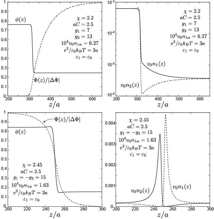
Figure 2: Top: normalized potential $\Phi(z)/\Delta\Phi$ (left), composition $\phi(z)$ (left), and normalized ion densities $v_{0}n_{1}(z)$ and $v_{0}n_{2}(z)$ (right on a semilogarithmic scale) for hydrophilic ion pairs, where $\chi=2.2,g_{1}=7,g_{2}=13$, $v_{0}n_{1\alpha}=v_{0}n_{1\beta}=4\times 10^{-4}$, and $e\Delta\Phi=-1.55k_{B}T$. Bottom: those for antagonistic ion pairs, where $\chi=2.45,g_{1}=15,g_{2}=-15$, $v_{0}n_{1\alpha}=v_{0}n_{1\beta}=1.63\times 10^{-4}$, and $e\Delta\Phi=10.3k_{B}T$. In these cases $e^{2}/\varepsilon_{0}k_{B}T=3a$ and $\varepsilon_{1}=\varepsilon_{0}$.

The upper plates give $\phi(z)$, $\Phi(z)$, $n_{1}(z)$, and $n_{2}(z)$ for hydrophilic ion pairs with $g_{1}=7$ and $g_{2}=13$ at $\chi=2.2$ and $n_{1\alpha}=n_{2\alpha}=4\times 10^{-4}v_{0}^{-1}$. The ion reduction factor in Eq.(3.9) is $0.0057$. The potential $\Phi$ varies mostly in the right side (phase $\beta$) on the scale of the Debye length $\kappa_{\beta}^{-1}=67.5a$ (which is much longer than that $\kappa_{\alpha}^{-1}=6.1a$ in phase $\alpha$). The Galvani potential difference $\Delta\Phi$ is $0.76k_{B}T/e$ here. The surface tension here is $\sigma=6.53\times 10^{-2}k_{B}T/a^{2}$ and is slightly larger than that $\sigma_{0}=6.22k_{B}T/a^{2}$ without ions (see the next subsection).

The lower plates display the same quantities for antagonistic ion pairs with $g_{1}=15$ and $g_{2}=-15$ for $\chi=2.45$ and $n_{1\alpha}=n_{2\alpha}=1.67\times 10^{-4}v_{0}^{-1}$. The anions and the cations are undergoing microphase separation at the interface on the scale of the Debye lengths $\kappa_{\alpha}^{-1}=12.3a$ and $\kappa_{\beta}^{-1}=9.70a$, resulting in a large electric double layer and a large potential drop ($\sim 10k_{B}T/e$). The surface tension here is $\sigma=0.0805k_{B}T/a^{2}$ and is about half of that $\sigma_{0}=0.155k_{B}T/a^{2}$ without ions. This large decrease in $\sigma$ is marked in view of small $n_{1\alpha}$. A large decrease of the surface tension was observed for an antagonistic salt Reid ; Luo

3.4 Surface tension. There have been numerous measurements of the surface tension of an air-water interface with a salt in the water region. In this case, almost all salts lead to an increase in the surface tension Onsager ; Levin-Flores , while acids tend to lower it because hydronium ions are trapped at an air-water interface.h1 ; Levinhyd

Here, we consider the surface tension of a liquid-liquid interface in our Ginzburg-Landau scheme, where ions can be present in the two sides of the interface. In equilibrium we minimize $\Omega=\int d{z}\omega$, where $\omega$ is the grand potential density,

$$\omega=f_{\rm tot}+\frac{1}{2}C|\nabla\phi|^{2}+\frac{\varepsilon}{8\pi}{\mbox{\boldmath$E$}}^{2}-h\phi-\sum_{i}\mu_{i}n_{i}.$$ (3.24)

Using Eqs.(3.10) and (3.11) we find $d(\omega+\rho\Phi)/dz=2C\phi^{\prime}\phi^{\prime\prime}$, where $\phi^{\prime}=d\phi/dz$ and $\phi^{\prime\prime}=d^{2}\phi/dz^{2}$. Thus,

$$\omega=C\phi^{\prime 2}-\rho\Phi+\omega_{\infty},$$ (3.25)

Since $\phi^{\prime}$ and $\rho$ tend to zero far from the interface, $\omega(z)$ tends to a common constant $\omega_{\infty}$ as $z\to\pm\infty$. The surface tension $\sigma=\int dz[\omega(z)-\omega_{\infty}]$ is then written as OnukiPRE ; OnukiJCP

$$\sigma=\int dz\bigg{[}C\phi^{\prime 2}-\frac{\varepsilon}{4\pi}{\mbox{\boldmath$E$}}^{2}\bigg{]}=2\sigma_{\rm g}-2\sigma_{\rm e},$$ (3.26)

where we introduce the areal densities of the gradient free energy and the electrostatic energy as

$$\sigma_{\rm g}=\int dz~{}C\phi^{\prime 2}/2,\quad\sigma_{\rm e}=\int dz~{}{\varepsilon}{\mbox{\boldmath$E$}}^{2}/{8\pi}.$$ (3.27)

The expression $\sigma=2\sigma_{\rm g}$ is well-known in the Ginzburg-Landau theory without the electrostatic interaction Onukibook .

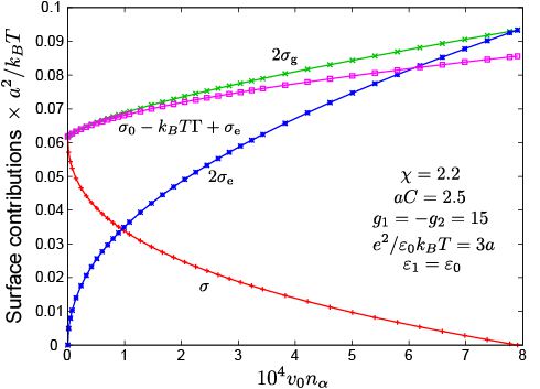
Figure 3: Surface quantities $\sigma$, $2\sigma_{\rm e}$, $2\sigma_{\rm g}$, and $\sigma_{0}-k_{B}T\Gamma+\sigma_{e}$ in units of $k_{B}Ta^{-2}$ vs $v_{0}n_{\alpha}$ for a monovalent, antagonistic salt with $g_{1}=-g_{2}=15$ at $\chi=2.4$. Here $2\sigma_{\rm g}$ and $\sigma_{0}-k_{B}T\Gamma+\sigma_{e}$ are close, supporting Eq.(3.30). Growth of $2\sigma_{\rm e}$ gives rise to vanishing of the surface tension $\sigma$ at $v_{0}n_{\alpha}=8\times 10^{-4}$.

In our previous work OnukiPRE ; OnukiJCP , we obtained the following approximate expression for $\sigma$ valid for small ion densities:

$$\sigma\cong\sigma_{0}-k_{B}T\Gamma-\sigma_{\rm e},$$ (3.28)

where $\sigma_{0}$ is the surface tension without ions and $\Gamma$ is the adsorption to the interface. In terms of the total ion density $n=n_{1}+n_{2}$, it may be expressed as

$$\Gamma=\int dz\bigg{[}n-n_{\alpha}-\frac{\Delta n}{\Delta\phi}(\phi-\phi_{\alpha})\bigg{]},$$ (3.29)

where $n_{K}=n_{1K}+n_{2K}$ ($K=\alpha$, $\beta$), $\Delta n=n_{\alpha}-n_{\beta}$, and the integrand tends to zero as $z\to\pm\infty$. From Eqs.(3.26) and (3.28) $\sigma_{\rm g}$ is expressed at small ion densities as

$$2\sigma_{\rm g}\cong\sigma_{0}-k_{B}T\Gamma+\sigma_{\rm e}.$$ (3.30)

In the Gibbs formula ($\sigma\cong\sigma_{0}-k_{B}T\Gamma$) Safran ; Gibbs , the electrostatic contribution $-\sigma_{\rm e}$ is neglected. However, it is crucial for antagonistic saltOnukiJCP ; Araki and for ionic surfactant OnukiEPL .

In Fig.3, numerical results of $2\sigma_{e}$, $2\sigma_{\rm g}$, $\sigma$, and the combination $\sigma_{0}-k_{B}T\Gamma+\sigma_{\rm e}$ are plotted as functions of the bulk ion density $n_{\alpha}=n_{1\alpha}+n_{2\alpha}$ for the antagonistic case $g_{1}=-g_{2}=15$, where $\chi=2.4$ and $C=2.5k_{B}T/a^{2}$. The parameter $\gamma_{\rm p}$ in Eq.(3.15) exceeds unity (being equal to 1.89 for $\varepsilon=1.5\varepsilon_{0}$). In this example, $\sigma_{\rm g}$ weakly depends on $n_{\alpha}$ and is fairly in accord with Eq.(3.30), while $\sigma_{\rm e}$ steeply increases with increasing $n_{\alpha}$. As a result, $\sigma_{\rm e}$ increases up to $\sigma_{\rm g}$, leading to vanishing of $\sigma$ at $n_{\alpha}\cong 8\times 10^{-4}v_{0}^{-1}$.

We may understand the behavior of $\sigma_{\rm e}$ as a function of $g_{1}$ and $g_{2}$ by solving the nonlinear Poisson-Boltzmann equation OnukiJCP , with an interface at $z=0$. That is, away from the interface $|z|>\xi$, the normalized potential $U(z)\equiv e\Phi(z)/k_{B}T$ obeys

$$\frac{d^{2}}{dz^{2}}U=\kappa_{K}^{2}\sinh(U-U_{K})$$ (3.31)

in the two phases ($K=\alpha$, $\beta$), where $U_{\alpha}=U(-\infty)$, $U_{\beta}=U(\infty)$, and $\kappa_{K}=(4\pi n_{K}e^{2}/\varepsilon_{K}k_{B}T)^{1/2}$ with $\varepsilon_{K}=\varepsilon_{0}+\varepsilon_{1}\phi_{K}$. In solving Eq.(3.31) we assume the continuity of the electric induction $-\varepsilon d\Phi/dz$ at $z=0$ (but this does not hold in the presence of interfacial orientation of molecular dipoles, as will be remarked in the summary section). The Poisson-Boltzmann approximation for $\sigma_{\rm e}$ is of the form,

$$\frac{\sigma_{\rm e}^{\rm\small{PB}}}{k_{B}T} = \frac{2n_{\alpha}}{\kappa_{\alpha}}\bigg{[}\sqrt{1+b^{2}+2b\cosh({\Delta U}/{2})}-b-1\bigg{]}$$ (3.32)

$$= A_{s}(n_{\alpha}/\ell_{{\rm B}\alpha})^{1/2}.$$

We should have $\sigma_{\rm e}\cong\sigma_{\rm e}^{\rm\small{PB}}$ in the thin interface limit $\xi\ll\kappa_{K}^{-1}$. In the first line, the coefficient $b$ is defined by

$$b=({\varepsilon_{\beta}/\varepsilon_{\alpha}})^{1/2}\exp[-({g_{1}+g_{2}})\Delta\phi/4],$$ (3.33)

and $\Delta U=U_{\alpha}-U_{\beta}=(g_{1}-g_{2})\Delta\phi/2$ is the normalized potential difference calculated from Eq.(3.8). In the second line, $\ell_{{\rm B}\alpha}=e^{2}/\varepsilon_{\alpha}k_{B}T$ is the Bjerrum length in phase $\alpha$. The second line indicates that the electrostatic contribution to the surface tension is negative and is of order ${n_{\alpha}}^{1/2}$ as ${n_{\alpha}}\to 0$ away from the solvent criticality, as first predicted by Nicols and Pratt for liquid-liquid interfaces Pratt . Remarkably, the surface tension of air-water interfaces exhibited the same behavior at very small salt densities (known as the Jones-Ray effect) Jones , though it has not yet been explained reliably OnukiJCP .

In the asymptotic limit of antagonistic ion pairs, we assume $g_{1}\geq-g_{2}\gg 1$, where the coefficient $A_{s}$ in the second line of eq.(3.32) grows as

$$A_{s}\cong\pi^{-1/2}(\varepsilon_{\beta}/\varepsilon_{\alpha})^{1/4}\exp({|g_{2}|\Delta\phi/4})$$ (3.34)

We may also examine the usual case of hydrophilic ion pairs in water-oil, where $g_{1}$ and $g_{2}$ are both considerably larger than unity. In this case $A_{s}$ becomes small as

$$A_{s} \cong ({\varepsilon_{\beta}/\pi\varepsilon_{\alpha}})^{1/2}[\cosh(\Delta U/2)-1]$$ (3.35)

$$\times\exp[-(g_{1}+g_{2})\Delta\phi/4].$$

In this case, the electrostatic contribution $-\sigma_{\rm e}(\propto n_{\alpha}^{1/2})$ in $\sigma$ could be detected only at extremely small salt densities.

Analogously, between ionic and nonionic liquids, Aerov el al. Aerov calculated the surface tension. They showed that if the affinities of cations and anions to neutral molecules are very different, the surface tension becomes negative.

3.5 Mesophase formation with antagonistic salt. Adding an antagonistic salt with $\gamma_{\rm p}>1$ to water-oil, we have found instability of one-phase states with increasing ${\chi}$ below Eq.(3.15) and vanishing of the surface tension $\sigma$ with increasing the ion content as in Fig.3. In such cases, a thermodynamic instability is induced with increasing $\chi$ at a fixed ion density $n_{0}=\langle{n_{1}}\rangle=\langle{n_{2}}\rangle$, leading to a mesophase. To examine this phase ordering, we performed two-dimensional simulations Araki ; Nara and presented an approximate phase diagram Nara . We here present preliminary three-dimensional results. The patterns to follow resemble those in block copolymers and surfactant systems Onukibook ; Seul . In our case, mesophases emerge due to the selective solvation and the Coulomb interaction without complex molecular structures. Solvation-induced mesophase formation can well be expected in polyelectrolytes and mixtures of ionic and polar liquids.

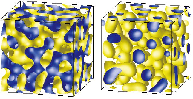
Figure 4: Composition patterns at $t=5000t_{0}$ for $\chi=2.1$ and $v_{0}{\bar{n}}=3\times 10^{-3}$ with average composition $\langle{\phi}\rangle$ being $0.5$ (left) and $0.4$ (right) for antagonistic salt with $g_{1}=-g_{2}=10$. These patterns are nearly pinned. Yellow surfaces are oriented to the regions of $\phi>0.5$ and blue ones are to those of $\phi<0.5$.

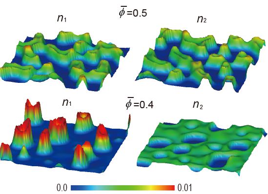
Figure 5: Cross-sectional profiles of cation $n_{1}$ (left) and anion $n_{2}$ (right) in the $x$-$y$ plane at $z=0$ for antagonistic salt using data in Fig. 4. The domains are bicontinuous for $\langle{\phi}\rangle=0.5$ (top) and droplet-like for $\langle{\phi}\rangle=0.4$ (bottom).

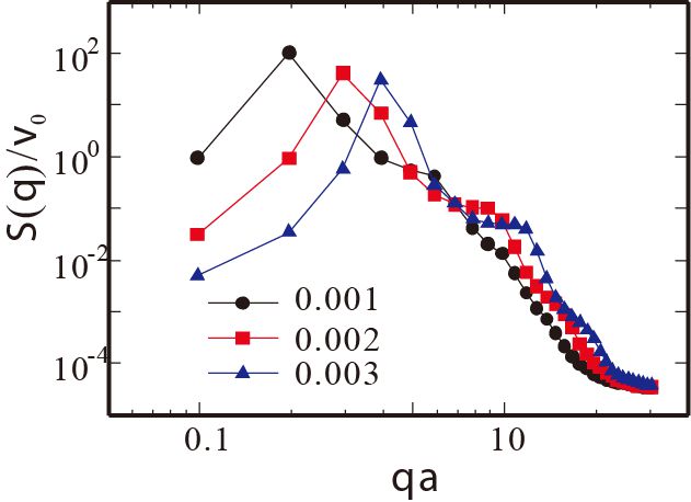
Figure 6: Normalized structure factor $S(q)/v_{0}$ for antagonistic salt from domain structures in pinned states at $t=5000t_{0}$, where the patterns are bicontinuous at for $\langle{\phi}\rangle=0.5$. A peak height $S(q_{m})/v_{0}$ of each curve much exceed unity. The average ion density is $v_{0}n_{0}=0.001,0.002$, and 0.003 for the three curves (from above for $q<q_{m}$).

We are interested in slow composition evolution with antagonistic ion pairs, so we assume that the ion distributions are given by the modified Poisson-Boltzmann relations in Eq.(3.12). The water composition $\phi$ obeys Araki ; Nara

$$\frac{\partial\phi}{\partial t}+\nabla\cdot(\phi\mbox{\boldmath$v$})=\frac{L_{0}}{k_{B}T}\nabla^{2}h,$$ (3.36)

where $L_{0}$ is the kinetic coefficient and $h$ is defined by Eq.(3.10). Neglecting the acceleration term, we determine the velocity field $v$ using the Stokes approximation,

$$\eta_{0}\nabla^{2}{\mbox{\boldmath$v$}}=\nabla p_{1}+\phi\nabla h+\sum_{i}n_{i}\nabla\mu_{i},$$ (3.37)

where $\eta_{0}$ is the shear viscosity and $\mu_{i}$ are defined by Eq.(3.11), We introduce $p_{1}$ to ensure the incompressibility condition $\nabla\cdot{\mbox{\boldmath$v$}}=0$. The right hand side of Eq.(3.37) is also written as $\nabla\cdot{\tensor{\Pi}}$, where ${\tensor{\Pi}}$ is the stress tensor arising from the fluctuations of $\phi$ and $n_{i}$. Here the total free energy $F$ in Eq.(3.1) satisfies $dF/dt\leq 0$ with these equations (if the boundary effect arising from the surface free energy is neglected).

We integrated Eq.(3.36) using the relations (3.4), (3.12), and (3.37) on a $64\times 64\times 64$ lattice under the periodic boundary condition. The system was quenched to an unstable state with $\chi=2.1$ at $t=0$. Space and time are measured in units of $a=v_{0}^{1/3}$ and $t_{0}=a^{5}/L_{0}$, respectively. Without ions, the diffusion constant of the composition is given by $L_{0}f^{\prime\prime}/k_{B}T$ in one-phase states in the long wavelength limit (see Eq.(3.14)). We set $g_{1}=-g_{2}=10$, ${n}_{0}=3\times 10^{-3}v_{0}^{-1}$, $C=k_{B}T/2a^{2}$, $e^{2}/\varepsilon_{0}k_{B}T=3a$, $\varepsilon_{1}=0$, and $\eta_{0}L_{0}/k_{B}T=0.16a^{4}$.

In Fig.4, we show the simulated domain patterns at $t=5000t_{0}$, where we can see a bicontinuous structure for $\langle{\phi}\rangle=0.5$ and a droplet structure for $\langle{\phi}\rangle=0.4$. There is almost no further time evolution from this stage. In Fig.5, the ion distributions are displayed for these two cases in the $x$-$y$ plane at $z=0$. For $\langle{\phi}\rangle=0.5$, the ion distributions are peaked at the interfaces forming electric double layers (as in the right bottom plate of Fig.2). For $\langle{\phi}\rangle=0.4$, the anions are broadly distributed in the percolated oil region, but we expect formation of electric double layers with increasing the domain size also in the off-critical condition. In Fig.6, the structure factor $S(q)$ in steady states are plotted for $v_{0}n_{0}=0.001,0.002$, and 0.003. The peak position decreases with increasing $n_{0}$ in accord with Eq.(3.16). Sadakane et al. Sadakane ; SadakanePRL observed the structure factor similar to those in Fig.6.

Finally, we remark that the thermal noise, which is absent in our simulation, should be crucial near the criticality of low-molecilar-weight solvents. It is needed to explain anomalously enhanced composition fluctuations induced by NaBPh₄ near the solvent criticalitySeto .

IV Ionic surfactant with amphiphilic and solvation interactions

4.1 Ginzburg-Landau theory. In this section, we will give a diffuse-interface model of ionic surfactantsOnukiEPL , where surfactant molecules are treated as ionized rods. Their two ends can stay in very different environments (water and oil) if they are longer than the interface thickness $\xi$. In our model, the adsorption of ionic surfactant molecules and counterions to an oil-water interface strongly depends on the selective solvation parameters $g_{1}$ and $g_{2}$ and that the surface tension contains the electrostatic contribution as in Eqs.(3.26) and (3.28).

We add a small amount of cationic surfactant, anionic counterions in water-oil in the monovalent case. The densities of water, oil, surfactant, and counterion are $n_{A}$, $n_{B}$, $n_{1}$, and $n_{2}$, respectively. The volume fractions of the first three components are $\phi_{A}=v_{0}n_{A}$, $\phi_{B}=v_{0}n_{B}$, and $v_{1}n_{1}$, where $v_{0}$ is the common molecular volume of water and oil and $v_{1}$ is the surfactant molecular volume. The volume ratio $N_{1}=v_{1}/v_{0}$ can be large, so we do not neglect the surfactant volume fraction, while we neglect the counterion volume fraction supposing a small size of the counterions. We assume the space-filling condition,

$$\phi_{A}+\phi_{B}+v_{1}n_{1}=1.$$ (4.1)

Let $2\psi=\phi_{A}-\phi_{B}$ be the composition difference between water and oil; then,

$$\phi_{A}=(1-v_{1}n_{1})/2+\psi,$$

$$\phi_{B}=(1-v_{1}n_{1})/2-\psi.$$ (4.2)

The total free energy $F$ is again expressed as in Eq.(3.1). Similarly to Eq.(3.2), the first part reads

$$\frac{f_{\rm tot}}{k_{B}T} = \frac{1}{v_{0}}[\phi_{A}\ln\phi_{A}+\phi_{B}\ln\phi_{B}+\chi\phi_{A}\phi_{B}]$$ (4.3)

$$+\sum_{i}n_{i}[\ln(n_{i}\lambda_{i}^{3})-g_{i}n_{i}\psi]-n_{1}\ln Z_{\rm a},$$

The coefficients $g_{1}$ and $g_{2}$ are the solvation parameters of the ionic surfactant and the counterions, respectively. Though a surfactant molecule is amphiphilic, it can have preference to water or oil on the average. The last term represents the amphiphilic interaction between the surfactant and the composition. That is, $Z_{\rm a}$ is the partition function of a rod-like dipole with its center at the position $r$. We assume that the surfactant molecules take a rod-like shape with a length $2\ell$ considerably longer than $a=v_{0}^{1/3}$. It is given by the following integral on the surface of a sphere with radius $\ell$,

$$Z_{\rm a}({\mbox{\boldmath$r$}})=\int\frac{{d\Omega}}{4\pi}\exp\bigg{[}w_{\rm a}\psi({\mbox{\boldmath$r$}}-\ell{\mbox{\boldmath$u$}})-w_{\rm a}\psi({\mbox{\boldmath$r$}}+\ell{\mbox{\boldmath$u$}})\bigg{]},$$ (4.4)

where $u$ is the unit vector along the rod direction and $\int d\Omega$ represents the integration over the angles of $u$. The two ends of the rod are at ${\mbox{\boldmath$r$}}+\ell{\mbox{\boldmath$u$}}$ and ${\mbox{\boldmath$r$}}-\ell{\mbox{\boldmath$u$}}$ under the influence of the solvation potentials given by $k_{B}Tw_{\rm a}\psi({\mbox{\boldmath$r$}}+\ell{\mbox{\boldmath$u$}})$ and $-k_{B}Tw_{\rm a}\psi({\mbox{\boldmath$r$}}-\ell{\mbox{\boldmath$u$}})$. The parameter $w_{\rm a}$ represents the strength of the amphiphilic interaction.

Adsorption is strong for large $w_{\rm a}\Delta\psi\gg 1$, where $\Delta\psi=\psi_{\alpha}-\psi_{\beta}(\cong\phi_{A\alpha}-\phi_{A\beta})$ is the difference of $\psi$ between the two phases $\alpha$ and $\beta$. In the one-dimensional case, all the quantities vary along the $z$ axis and $Z_{\rm a}$ is rewritten as

$$Z_{\rm a}(z)=\int_{-\ell}^{\ell}\frac{{d\zeta}}{2\ell}\exp[w_{\rm a}\psi(z-\zeta)-w_{\rm a}\psi(z+\zeta)].$$ (4.5)

where $\zeta=\ell u_{z}$. In the thin interface limit $\xi\ll\ell$, we place the interface at $z=0$ to find $Z_{\rm a}=1$ for $|z|>\ell$, while

$$Z_{\rm a}(z)\cong 1+({1-|z|/\ell})[\cosh({w_{\rm a}\Delta\psi})-1],$$ (4.6)

for $|z|<\ell$. Furthermore, in the dilute limit $v_{1}n_{1}\ll 1$ and without the electrostatic interaction, we have $n_{1}(z)=n_{1\alpha}Z_{\rm a}(z)$ for $z<0$ and $n_{1}(z)=n_{1\beta}Z_{\rm a}(z)$ for $z>0$, where $n_{1\alpha}$ and $n_{1\beta}=e^{-g_{1}\Delta\psi}n_{1\alpha}$ are the bulk surfactant densities. The surfactant adsorption then grows as

$$\Gamma_{1} =\int_{-\infty}^{0}dz[n_{1}(z)-n_{\alpha}]+\int_{0}^{\infty}dz[n_{1}(z)-n_{\beta}]$$ (4.7)

$$=(n_{1\alpha}+n_{1\beta})\ell[\cosh({w_{\rm a}\Delta\psi})-1]/2.$$

However, the steric effect comes into play at the interface with increasing the surfactant volume fraction at the interface ($\sim\Gamma_{1}v_{1}/\ell$).

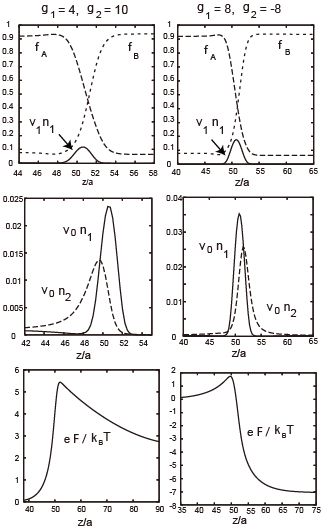
Figure 7: Profiles for mixtures with cationic surfactant and anionic counterions with $v_{1}=5v_{0}$ and $w_{\rm a}=12$. Top: $v_{1}n_{1}$ (bold line), $\phi_{A}$, and $\phi_{B}$. Middle: $v_{0}n_{1}$ and $v_{0}n_{2}$. Bottom: $e\Phi/k_{B}T$ exhibiting a maximum at the interface. Here $g_{1}=4$, $g_{2}=10$, and $v_{0}n_{1\alpha}=10^{-3}$ (left), while $g_{1}=-g_{2}=8$ and $v_{0}n_{1\alpha}=3.6\times 10^{-4}$ (right). The counterion distribution has a peak in the phase $\alpha$ (left) or $\beta$ (right) depending on $g_{2}$. $[$From: A. Onuki, Europhys. Lett. 82, 58002 (2008)$]$.

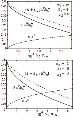
Figure 8: $\sigma a^{2}/k_{B}T$, $(\sigma+\sigma_{\rm e})a^{2}/k_{B}T$, and $\Gamma a^{2}$ as functions of $v_{0}n_{1\alpha}$ with $v_{1}=5v_{0}$, $\chi=3$, and $w_{\rm a}=12$. The curves change on a scale of $10^{-3}$ for hydrophilic ion pair $g_{1}=4$ and $g_{2}=10$ (top) and on a scale of $10^{-4}$ for antagonistic ion pair $g_{1}=-g_{2}=8$ (bottom). $[$From: A. Onuki, Europhys. Lett. 82, 58002 (2008)$]$.

4.2 Interface profiles of compositions, ion densities, and potential. We give typical one-dimensional interface profiles varying along the $z$-axis in Fig.7. We set $v_{1}=5v_{0}$, $C=3k_{B}T/a$, $\chi=3$, and $e^{2}/a\varepsilon_{c}k_{B}T=16/\pi$. The dielectric constant is assumed to be of the form $\varepsilon=\varepsilon_{c}(1+0.8\psi)$, where $\varepsilon_{c}$ is the critical value. Then $\varepsilon_{\alpha}\cong 2\varepsilon_{\beta}$ at $\chi=3$. This figure was produced in the presence of the image interaction in our previous workOnukiEPL (though it is not essential here).

In Fig.7, we show the volume fractions $\phi_{A}$, $\phi_{B}$, and $v_{1}n_{1}=1-\phi_{A}-\phi_{B}$ (top), the ion densities $n_{1}$ and $n_{2}$ (middle), and the potential $e\Phi/k_{B}T$ with $\Phi_{\alpha}=0$ (bottom). In the left, the counterions are more hydrophilic than the cationic surfactant, where $g_{1}=4$ and $g_{2}=10$ leading to $\Gamma=0.124a^{-2}$ and $\sigma=0.317k_{B}Ta^{-2}$ at $n_{1\alpha}=10^{-3}v_{0}^{-1}$. In the right plates, the surfactant cations are hydrophilic and the counterions are hydrophobic, where $g_{1}=-g_{2}=8$ leading to $\Gamma=0.155a^{-2}$ and $\sigma=0.159k_{B}Ta^{-2}$ at $n_{1\alpha}=3.6\times 10^{-4}v_{0}^{-1}$. The distribution of the surfactant $n_{1}$ is narrower than that of the counterions $n_{2}$. This gives rise to a peak of $\Phi$ at $z=z_{\rm p}$, at which $E(z_{\rm p})\propto\int_{-\infty}^{z_{\rm p}}dz(n_{1}(z)-n_{2}(z))=0$.

The adsorption strongly depends on the solvation parameters $g_{1}$ and $g_{2}$. It is much more enhanced for antagonistic ion pairs than for hydrophilic ion pairs.

4.3 Surface tension. The grand potential density $\omega$ is again given by Eq.(3.24) and tends to a common constant $\omega_{\infty}$ as $z\to\pm\infty$, though its form is more complicated. The surface tension $\sigma=\int dz[\omega(z)-\omega_{\infty}]$ is rewritten as Eq.(3.26) and is approximated as Eq.(3.28) for small $n_{1\alpha}$. The areal electrostatic-energy density $\sigma_{\rm e}$ in Eq.(3.27) is again important in the present case.

In Fig.8, we show $\sigma$, $\sigma+\sigma_{\rm e}$, and $\Gamma$ as functions of $v_{0}n_{1\alpha}$ at $w_{\rm a}=12$, where $\Gamma$ is defined as in Eq.(3.28) for $n=n_{1}+n_{2}$. In the upper plate, the two species of ions are both hydrophilic ($g_{1}=4$ and $g_{2}=10$), while in the lower plate the surfactant and the counterions are antagonistic ($g_{1}=8$ and $g_{2}=-8$). For the latter case, a large electric double layer is formed at an interface, leading to a large $\Gamma$ and a large decrease in $\sigma$ even at very small $n_{1\alpha}$. In the present case the Gibbs term $k_{B}T\Gamma$ is a few times larger than $\sigma_{\rm e}$. Note that the approximate formula (3.28) may be derived also in this case, but it is valid only for very small $n_{1\alpha}$ in Fig.8.

V Phase separation due to strong selective solvation

5.1 Strongly hydrophilic or hydrophobic solute. With addition of a strongly selective solute in a binary mixture in one-phase states, we predict precipitation of domains composed of the preferred component enriched with the soluteOkamoto . These precipitation phenomena occur both for a hydrophilic salt (such as NaCl) and a neutral hydrophobic solute S1 ; S2 ; S3 ; S4 ; S5 ; S6 ; S7 . In our scheme, a very large size of the selective solvation parameter $g_{i}$ is essential. In Secs.2 and 3, we have shown that $|g_{i}|$ can well exceed $10$ both for hydrophilic and hydrophobic solutes.

With hydrophilic cations and anions, a charge density appears only near the interfaces, shifting the surface tension slightly. Thus, in the static aspect of precipitation, the electrostatic interaction is not essential, while fusion of precipitated domains should be suppressed by the presence of the electric double layers. We will first treat a hydrophilic neutral solute as a third component, but the following results are applicable also to a neutral hydrophobic solute if water and oil are exchanged. In addition, in a numerical example in Fig.11, we will include the electrostatic interaction among hydrophilic ions.

5.2 Conditions of two phase coexistence. Adding a small amount of a highly selective solute in water-oil, we assume the following free energy density,

$${f}_{\rm tot}(\phi,n)=f(\phi)+k_{B}T{n}[\ln(n\lambda^{3})-1-g\phi].$$ (5.1)

This is a general model for a dilute solute. For monovalent electrolytes, this form follows from Eq.(3.11) if there is no charge density or if we set

$$n_{1}=n_{2}=n/2,\quad g=(g_{1}+g_{2})/2,$$ (5.2)

The first term $f(\phi)$ is assumed to be of the Bragg-Williams form (3.3). The $\lambda$ is the thermal de Broglie length. The solvation term ($\propto g$) arises from the solute preference of water over oil (or oil over water). The strength $g$ is assumed to much exceed unityOnukiPRE . We fix the amounts of the constituent components in the cell with a volume $V$. Then the averages $\bar{\phi}=\langle{\phi}\rangle=\int d{\mbox{\boldmath$r$}}\phi/V$ and ${\bar{n}}=\langle{n}\rangle=\int d{\mbox{\boldmath$r$}}n/V$ are given control parameters as well as $\chi$.

In two phase coexistence in equilibrium, let the composition and the solute density be $(\phi_{\alpha},n_{\alpha})$ in phase $\alpha$ and $(\phi_{\beta},n_{\beta})$ in phase $\beta$, where $\phi_{\alpha}>{\bar{\phi}}>\phi_{\beta}$ and $n_{\alpha}>{\bar{n}}>n_{\beta}$. We introduce the chemical potentials $h={\partial f_{\rm tot}}/{\partial\phi}$ and $\mu={\partial f_{\rm tot}}/{\partial n}$. Equation (5.1) yields

$$h=f^{\prime}(\phi)-k_{B}Tgn,$$ (5.3)

$$\mu/k_{B}T=\ln(n\lambda^{3})-g\phi,$$ (5.4)

where $f^{\prime}=\partial f/\phi$. The system is linearly stable for $\partial h/\partial\phi-(\partial h/\partial n)^{2}/\partial\mu/\partial n>0$ or for

$$f^{\prime\prime}(\phi)-k_{B}Tg^{2}n>0,$$ (5.5)

where $f^{\prime\prime}=\partial^{2}f/\partial\phi^{2}$. Spinodal decomposition occurs if the left hand side of Eq.(5.5) is negative.

The homogeneity of $\mu$ yields

$$n={\bar{n}}e^{g\phi}/\langle{e^{g\phi}}\rangle,$$ (5.6)

where $\langle{\cdots}\rangle$ denotes taking the space average. The bulk solute densities are $n_{K}={\bar{n}}e^{g\phi_{K}}/\langle{e^{g\phi}}\rangle$ for $K=\alpha,\beta$ in two-phase coexistence. In our approximation Eq.(5.6) holds even in the interface regions. We write the volume fraction of phase $\alpha$ as $\gamma_{\alpha}$. We then have $\langle{e^{g\phi}}\rangle=\gamma_{\alpha}e^{g\phi_{\alpha}}+(1-\gamma_{\alpha})e^{g\phi_{\beta}}$ in Eq.(5.6). In terms of $\bar{\phi}$ and $\bar{n}$, $\gamma_{\alpha}$ is expressed as

$$\gamma_{\alpha}=({{\bar{\phi}}-\phi_{\beta}})/{\Delta\phi}=({{\bar{n}}-n_{\beta}})/{\Delta n}.$$ (5.7)

where $\Delta\phi=\phi_{\alpha}-\phi_{\beta}>0$ and $\Delta n=n_{\alpha}-n_{\beta}>0$. In these expressions we neglect the volume of the interface regions. Since $n_{\alpha}/n_{\beta}=e^{g\Delta\phi}\gg 1$ for $g\Delta\phi\gg 1$, the solute is much more enriched in phase $\alpha$ than in phase $\beta$. Eliminating $n$ using Eq.(5.6), we may express the average free energy density as

$$\langle{f_{\rm tot}}\rangle=\langle{f}\rangle-k_{B}T{\bar{n}}\ln[\langle{e^{g\phi}}\rangle]+A_{1},$$ (5.8)

where $A_{1}=k_{B}T{\bar{n}}[\ln({\bar{n}}\lambda^{3})-1]$ is a constant at fixed $\bar{n}$. In terms of $\phi_{\alpha}$, $\phi_{\beta}$, and $\gamma_{\alpha}$, Eq.(5.8) is rewritten as

$$\langle{f_{\rm tot}}\rangle = [\gamma_{\alpha}f(\phi_{\alpha})+(1-\gamma_{\alpha})f(\phi_{\beta})]$$ (5.9)

$$-k_{B}T{\bar{n}}\ln[\gamma_{\alpha}e^{g\phi_{\alpha}}+(1-\gamma_{\alpha})e^{g\phi_{\beta}}]+A_{1}.$$

The second term ($\propto{\bar{n}})$ is relevant for large $g$ (even for small $\bar{n}$). Now we should minimize $\langle{f_{\rm tot}}\rangle-h[\gamma_{\alpha}\phi_{\alpha}+(1-\gamma_{\alpha})\phi_{\beta}-\bar{\phi}]$ with respect to $\phi_{\alpha}$, $\phi_{\beta}$, and $\gamma_{\alpha}$ at fixed $\bar{\phi}$, where $h$ appears as the Lagrange multiplier. Then we obtain the equilibrium conditions of two-phase coexistence,

$$h=f^{\prime}(\phi_{\alpha})-k_{B}Tgn_{\alpha}=f^{\prime}(\phi_{\beta})-k_{B}Tgn_{\beta},$$ (5.10)

$${f(\phi_{\alpha})-f(\phi_{\beta})}-k_{B}T\Delta n=h{\Delta\phi}.$$ (5.11)

These static relations hold even for ion pairs under Eq.(5.2).

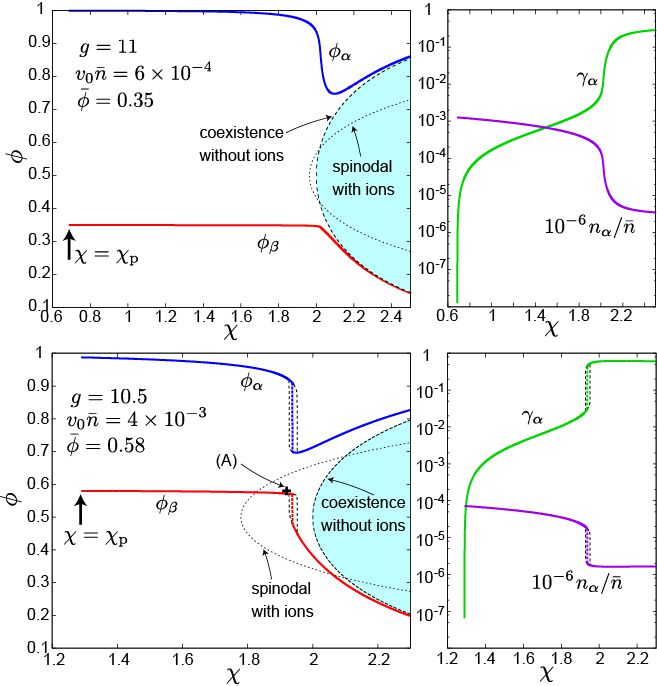
Figure 9: Left: compositions $\phi_{\alpha}$ and $\phi_{\beta}$ vs $\chi$. Right: semi-logarithmic plots of volume fraction $\gamma_{\alpha}$ and normalized solute density $n_{\alpha}/{\bar{n}}$ of the water-rich phase $\alpha$ vs $\chi$. Here $g=11$, ${\bar{\phi}}=0.35$, and ${\bar{n}}=6\times 10^{-4}v_{0}^{-1}$ (top), while $g=10.5$, ${\bar{\phi}}=0.58$, and ${\bar{n}}=4\times 10^{-3}v_{0}^{-1}$ (bottom). Plotted in the left also are the coexisting region without solute (in right green) and the spinodal curve with solute (on which the left hand side of Eq.(5.5) vanishes). See Fig.11 for simulation of phase separation on point (A) in the left bottom panel. $[$Upper plates are from: R. Okamoto and A. Onuki, Phys. Rev. E 82, 051501 (2010).$]$

5.3 Numerical results of two phase coexistence. In Fig.9, we give numerical results on the phase behavior of $\phi_{\alpha}$ and $\phi_{\beta}$ in the left and $n_{\alpha}$ and $\gamma_{\alpha}$ in the right as functions of $\chi$. We set $g=11$, $\bar{\phi}=0.35$ and ${\bar{n}}=6\times 10^{-4}v_{0}^{-1}$ in the top plates and $g=10.5$, ${\bar{\phi}}=0.58$, and ${\bar{n}}=4\times 10^{-3}v_{0}^{-1}$ in the bottom plates. The solute density is much larger in the latter case. Remarkably, a precipitation branch appears in the range,

$$\chi_{\rm p}<\chi<2.$$ (5.12)

The volume fraction $\gamma_{\alpha}$ decreases to zero as $\chi$ approaches the lower bound $\chi_{\rm p}=\chi_{\rm p}({\bar{\phi}},{\bar{n}})$. Without solute, the mixture would be in one-phase states for $\chi<2$. The precipitated domains are solute-rich with $\phi_{\alpha}\cong 1$, while $\phi_{\beta}$ is slightly larger than $\bar{\phi}$. In the left upper plate $\phi_{\alpha}$ increases continuously with decreasing $\chi$, while in the left lower plate $\phi_{\alpha}$ jumps at $\chi=1.937$ and hysteresis appears in the region $1.927<\chi<1.952$. We also plot the spinodal curve, $f^{\prime\prime}({\bar{\phi}})-k_{B}Tg^{2}{\bar{n}}=0,$ following from Eq.(5.5). Outside this curve, homogeneous states are metastable and precipitation can proceed via homogeneous nucleation in the bulk or via heterogeneous nucleation on hydrophilic surfaces of boundary plates or colloids Okamoto . Inside this curve, the system is linearly unstable and precipitation occurs via spinodal decomposition. This unstable region is expanded for ${\bar{n}}=4\times 10^{-3}v_{0}^{-1}$ in the lower plate.

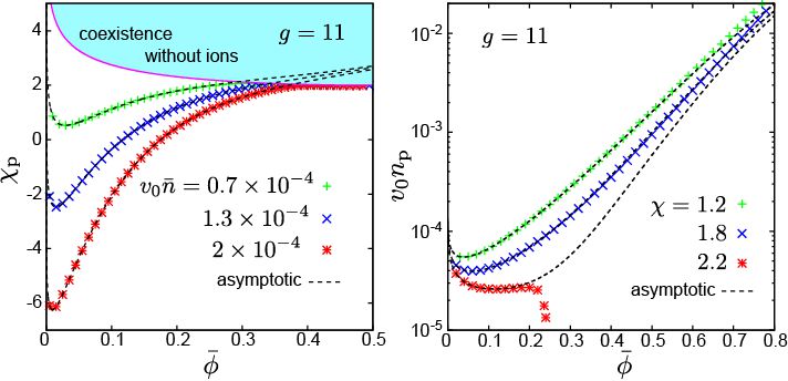
Figure 10: Left:$\chi_{\rm p}(\bar{\phi},{\bar{n}})$ vs $\bar{\phi}$ for three values of ${\bar{n}}$ at $g=11$, which nearly coincide with the asymptotic formula (5.22) (dotted line) for $\bar{\phi}<0.35$ and converge to the coexistence curve for larger $\bar{\phi}$. Coexistence region without ions is in the upper region (in right green). Right: $v_{0}n_{\rm p}(\bar{\phi},\chi)$ vs $\bar{\phi}$ on a semi-logarithmic scale at $g=11$, It coincides with the asymptotic formula (5.23) (dotted line) for $\chi<2$ and tends to zero at the coexistence composition, 0.249 (top) or 0.204 (bottom). $[$From: R. Okamoto and A. Onuki, Phys. Rev. E 82, 051501 (2010).$]$

5.4 Theory of asymptotic behavior for large $g$. We present a theory of the precipitation branch in the limit $g\gg 1$ to determine $\chi_{\rm p}$ and $n_{\rm p}$. Assuming the branch (5.12) at the starting point, we confirm its existence self-consistently.

We first neglect the term $-k_{B}Tgn_{\beta}$ in Eq.(5.10) from $gv_{0}n_{\beta}\ll 1$ and the term $f(\phi_{\alpha})$ in Eq.(5.11) from $\phi_{\alpha}\cong 1$. In fact $gv_{0}n_{\beta}\ll 1$ in Fig.9. We then obtain

$$h\cong f^{\prime}(\phi_{\beta})\cong-[{f(\phi_{\beta})+k_{B}Tn_{\alpha}}]/({1-\phi_{\beta}}).$$ (5.13)

This determines the solute density $n_{\alpha}$ in phase $\alpha$ as a function of $\phi_{\beta}$ in the form,

$$n_{\alpha}\cong G(\phi_{\beta})/k_{B}T,$$ (5.14)

where $G(\phi)$ is a function of $\phi$ defined as

$$G(\phi) = -f(\phi)-(1-\phi)f^{\prime}(\phi)$$ (5.15)

$$= -(k_{B}T/v_{0})[\ln\phi+\chi(1-\phi)^{2}].$$

From $dG/d\phi=-(1-\phi)f^{\prime\prime}(\phi)<0$ and $G(1)=0$, we have $G(\phi)>0$ outside the coexistence curve, ensuring $n_{\alpha}>0$ in Eq.(5.14).

In Eq.(5.10), we next use Eq.(3.3) for $f^{\prime}(\phi_{\alpha})$ to obtain

$$v_{0}^{-1}k_{B}T[-\ln(1-\phi_{\alpha})-\chi-gv_{0}n_{\alpha}]\cong f^{\prime}(\phi_{\beta}),$$ (5.16)

where the logarithmic term ($\propto\ln(1-\phi)$) balances with the solvation term ($\propto gn_{\alpha}$). Use of Eq.(5.15) gives

$${1-\phi_{\alpha}}\cong A_{\beta}\exp[-gv_{0}G(\phi_{\beta})/k_{B}T],$$ (5.17)

where the coefficient $A_{\beta}$ is given by

$$A_{\beta}=\exp[-\chi-v_{0}f^{\prime}(\phi_{\beta})/k_{B}T],$$ (5.18)

so $A_{\beta}$ is of order unity. The factor $\exp[-gv_{0}G(\phi_{\beta})/k_{B}T]$ in Eq.(5.17) is very small for $g\gg 1$, leading to $\phi_{\alpha}\cong 1$.

Furthermore, from Eqs.(5.6) and (5.7), the volume fraction $\gamma_{\alpha}$ of phase $\alpha$ is approximated as

$$\gamma_{\alpha}\cong{\bar{n}}/n_{\alpha}-e^{-g\Delta\phi}\cong k_{B}T{\bar{n}}/G(\phi_{\beta})-e^{-g\Delta\phi}.$$ (5.19)

The above relation is rewritten as

$$G(\phi_{\beta})\cong{k_{B}T{\bar{n}}}/{(\gamma_{\alpha}+e^{-g\Delta\phi})}$$

$$\cong\frac{k_{B}T{\bar{n}}(1-\phi_{\beta})}{\bar{\phi}-\phi_{\beta}+(1-\phi_{\beta})\exp[{-g(1-\phi_{\beta})]}}.$$ (5.20)

From the first to second line, we have used Eq.(5.7) and replaced $\Delta\phi$ by $1-\phi_{\beta}$. This equation determines $\phi_{\beta}$ and $\gamma_{\alpha}\cong({\bar{\phi}}-\phi_{\beta})/(1-\phi_{\beta})$. We recognize that $G(\phi_{\beta})$ increases up to $T{\bar{n}}e^{g\Delta\phi}\cong T{\bar{n}}e^{g(1-{\bar{\phi}})}$ as $\gamma_{\alpha}\to 0$ or as $\phi_{\beta}\to\bar{\phi}$. In this limit it follows the marginal relation,

$$G({\bar{\phi}})\cong k_{B}T{\bar{n}}e^{g(1-{\bar{\phi}})}\quad(\gamma_{\alpha}\to 0).$$ (5.21)

If ${\bar{n}}$ is fixed, this relation holds at ${\chi}=\chi_{\rm p}$ so that

$$\chi_{\rm p}\cong[-\ln\bar{\phi}-v_{0}{\bar{n}}e^{g(1-\bar{\phi})}]/(1-\bar{\phi})^{2},$$ (5.22)

where we use the second line of Eq.(5.15). Here $\bar{n}$ appears in the combination ${\bar{n}}e^{g(1-\bar{\phi})}(\gg{\bar{n}})$. On the other hand, if $\chi$ is fixed, Eq.(5.21) holds at ${\bar{n}}=n_{\rm p}$. Thus the minimum solute density $n_{\rm p}$ is estimated as

$$n_{\rm p}\cong e^{-g(1-{\bar{\phi}})}G({\bar{\phi}})/k_{B}T,$$ (5.23)

which is much decreased by the small factor $e^{-g(1-{\bar{\phi}})}$.

In Fig.10, the curves of $\chi_{\rm p}$ and $n_{\rm p}$ nearly coincide with the asymptotic formulas (5.22) and (5.23) in the range ${\bar{\phi}}<0.35$ for $\chi_{\rm p}$ and in the range $\chi<2$ for ${n}_{\rm p}$. They exhibit a minimum at $\bar{\phi}\sim e^{-g}/v_{0}{\bar{n}}g$ for $\chi_{\rm p}$ and at $\bar{\phi}\sim g^{-1}$ for ${n}_{\rm p}$. For larger $\bar{\phi}>0.35$, $\chi_{\rm p}$ nearly coincide with the coexistence curve, indicating disappearance of the precipitation branch. Notice that ${n}_{\rm p}$ decreases to zero as $\bar{\phi}$ approaches the coexistence composition $\phi_{\rm cx}=0.249$ at $\chi=2.2$ (top) and 0.204 at $\chi=2.3$ (bottom), where phase separation occurs without solute.

5.5 Simulation of spinodal decomposition for hydrophilic ions. In our theory Okamoto we investigated solute-induced nucleation starting with homogeneous metastable states outside the spinodal curve (dotted line) in the left panels of Fig.9. Here, we show two-dimensional numerical results of spinodal decomposition for hydrophilic ions with $g_{1}=12$, $g_{2}=9$, $e^{2}/\varepsilon_{0}k_{B}T=3a$, and $\varepsilon_{1}=\varepsilon_{0}$. At $t=0$, we started with point (A) inside the spinodal curve in the left lower panel in Fig.9 using the common values of the static parameters given by $\chi=1.92$, ${\bar{\phi}}=0.58$, and ${\bar{n}}=\langle{n_{1}+n_{2}}\rangle=4\times 10^{-3}/v_{0}$. In addition, we set $C=2k_{B}Ta^{2}/v_{0}$. On a $256\times 256$ lattice under the periodic boundary condition, we integrated Eq.(3.36) for the composition $\phi({\mbox{\boldmath$r$}},t)$ with the velocity field ${\mbox{\boldmath$v$}}({\mbox{\boldmath$r$}},t)$ being determined by the Stokes approximation in Eq.(3.37). The cations and anions obey

$$\frac{\partial n_{i}}{\partial t}+\nabla\cdot(n_{i}\mbox{\boldmath$v$})=\frac{D}{k_{B}T}\nabla\cdot n\nabla\mu_{i}$$

$$=D\nabla\cdot\bigg{[}{\nabla{n_{i}}}-g_{i}n_{i}\nabla\phi-Z_{i}en_{i}{\mbox{\boldmath$E$}}\bigg{]},$$ (5.24)

where $i=1,2$. The chemical potentials $\mu_{i}$ are defined in Eq.(3.11) and the ion diffusion constants are commonly given by $D$. The space mesh size is $a=v_{0}^{1/d}$ with $d=2$. We measure time in units of $t_{0}=a^{2}v_{0}/L_{0}$ and set $D=a^{2}/t_{0}$ and $\eta_{0}=0.15k_{B}Tt_{0}/v_{0}$, where $L_{0}$ is the kinetic coefficient for the composition and $\eta_{0}$ is the shear viscosity.

In Fig.11, we show the time evolution of the droplet volume fraction, which is the fraction of the region $\phi>0.6$. In the early stage, the droplet number decreases in time with the evaporation and condensation mechanism. In the late stage, it changes very slowly tending to a constant. In our simulation without random noise, the droplets do not undergo Brownian motion and the droplet collision is suppressed. We also performed a simulation for a neutral solute with $g=10.5$ (not shown here), which exhibits almost the same phase separation behavior as in Fig.11.

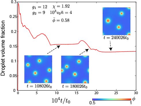
Figure 11: Time evolution of droplet volume fraction (that of the region $\phi>0.6$) and composition snapshots of precipitated droplets at three times. They are induced by hydrophilic ions with $g_{1}=12$ and $g_{1}=9$. The initial state was at point (A) in Fig.9 with $\chi=1.92$, ${\bar{\phi}}=0.58$, and ${\bar{n}}=4\times 10^{-3}v_{0}^{-1}$. The droplet volume fraction nearly tends to a constant.

VI Theory of polyelectrolytes

6.1 Weakly ionized polyelectrolytes. In this section, we consider weakly charged polymers in a theta or poor, one-component water-like solvent in the semidilute case $\phi>N^{-1/2}$. Following the literature of polymer physics PG , we use $\phi$ and $N$ to represent the polymer volume fraction and the polymerization index. Here charged particles interact differently between uncharged monomers and solvent molecules. The selective solvation should become more complicated for mixture solvents, as discuused in Sec.1.

To ensure flexibility of the chains, we assume that the fraction of charged monomers on the chains, denoted by $f_{\rm ion}$, is small or $f_{\rm ion}\ll 1$. From the scaling theoryPG , the polymers consist of blobs with monomer number $g_{b}=\phi^{-2}$ with length $\xi_{b}=ag_{b}^{1/2}=a\phi^{-1}$. The electrostatic energy within a blob is estimated as

$$\epsilon_{b}=k_{B}T(f_{\rm ion}g)^{2}\ell_{B}/\xi_{b}=k_{B}Tf_{\rm ion}^{2}\ell_{B}/\phi^{3}a.$$ (6.1)

where $\ell_{B}$ is the Bjerrum length. The blobs are not much deformed under the weak charge condition $\epsilon_{b}<k_{B}T$, which is rewritten as

$$\phi>f_{\rm ion}^{2/3}(\ell_{B}/a)^{1/3}.$$ (6.2)

6.2 Ginzburg-Landau theory. The number of the ionizable monomers (with charge $-e$) on a chain is written as $\nu_{M}N$ with $\nu_{M}<1$. Then the degree of ionization (or dissociation) is $\zeta=f_{\rm ion}/\nu_{M}$ and the number density of the ionized monomers is

$$n_{p}=v_{0}^{-1}f_{\rm ion}\phi=v_{0}^{-1}\nu_{M}\zeta\phi,$$ (6.3)

The charge density is expressed as

$$\rho=e\sum_{i=c,1,2}Z_{i}n_{i}-en_{p}.$$ (6.4)

Here $i=c$ represents the counterions, $i=1$ the added cations, and $i=2$ the added anions. The required relation $f_{\rm ion}\ll 1$ becomes $\nu_{M}\zeta\ll 1$ (which is satisfied for any $\zeta$ if $\nu_{M}\ll 1$).

We set up the free energy $F$ accounting for the molecular interactions and the ionization equilibriumOnuki-Okamoto . Then $F$ assumes the standard form (3.1), where the coefficient of the gradient free energy is written as Onukibook ; PG

$$C(\phi)=k_{B}T/12a\phi(1-\phi),$$ (6.5)

in terms of the molecular length $a=v_{0}^{1/3}$ and $\phi$. The $f_{\rm tot}$ consists of four parts as

$${f_{\rm tot}} = {f(\phi)}+{k_{B}T}\sum_{i=c,1,2}{n_{i}}[\ln(n_{i}\lambda_{i}^{3})-1+g_{i}\phi]$$ (6.6)

$$+{k_{B}T}(\Delta_{0}+g_{p}\phi)n_{p}+f_{\rm dis}.$$

The first term $f$ is of the Flory-Huggins form PG ; Onukibook ,

$$\frac{v_{0}f}{k_{B}T}=\frac{\phi}{N}\ln\phi+(1-\phi)\ln(1-\phi)+\chi\phi(1-\phi).$$ (6.7)

The coupling terms ($\propto g_{i},g_{p}$) arise from the molecular interactions among the charged particles (the ions and the charged monomers) and the uncharged particles (the solvent particles and the uncharged monomers), while $k_{B}T\Delta_{0}$ is the dissociation free energy in the dilute limit of polymers ($\phi\to 0$). The last term in $f_{\rm tot}$ arises from the dissociation entropy on chains Joanny ; Bu1 ; Bu2 ,

$$\frac{v_{0}}{k_{B}T}f_{\rm dis}={\nu_{M}}\phi\bigg{[}\zeta\ln\zeta+(1-\zeta)\ln(1-\zeta)\bigg{]}.$$ (6.8)

6.3 Dissociation equilibrium. If $F$ is minimized with respect to $\zeta$, it follows the equation of ionization equilibrium or the mass action law,

$$n_{c}{\zeta}/({1-\zeta})=K(\phi),$$ (6.9)

where $n_{c}$ is the counter ion density and $K(\phi)$ is the dissociation constant of the form,

$$K(\phi)=v_{0}^{-1}\exp[-\Delta_{0}-(g_{p}+g_{c})\phi].$$ (6.10)

We may interpret $k_{B}T[\Delta_{0}+(g_{p}+g_{c})\phi]$ as the composition-dependent dissociation free energy. With increasing the polymer volume fraction $\phi$, the dissociation decreases for positive $g_{p}+g_{c}$ and increases for negative $g_{p}+g_{c}$. If $g_{p}+g_{c}\gg 1$, $K(\phi)$ much decreases even for a small increase of $\phi$. Here $K(\phi)$ has the meaning of the crossover counterion density since $\zeta$ is expressed as

$$\zeta={1}/[1+n_{c}/K(\phi)],$$ (6.11)

which decreases appreciably for $n_{c}>K(\phi)$.

In particular, if there is no charge density and no salt ($n_{p}=n_{c}$ and $n_{1}=n_{2}=0$), $n_{c}$ satisfies the quadratic equation $n_{c}({n_{c}+K})=v_{0}^{-1}\nu_{M}\phi K,$ which is solved to give

$$\zeta={v_{0}n_{c}}/{\nu_{M}\phi}={2}/({\sqrt{Q(\phi)+1}+1}).$$ (6.12)

Here it is convenient to introduce

$$Q(\phi)={4\nu_{M}\phi}/{v_{0}K(\phi)}.$$ (6.13)

We find $\zeta\ll 1$ and $n_{c}\cong(\nu_{M}\phi K/v_{0})^{1/2}$ for $Q\gg 1$, while $\zeta\rightarrow 1$ for $Q\ll 1$. The relation (6.12) holds approximately for small charge densities without salt.

6.4 Structure factor. As in Sec.3, it is straightforward to calculate the structure factor $S(q)$ for the fluctuations of $\phi$ on the basis of $f_{\rm tot}$ in Eq.(6.6). As a function of the wave number $q$, it takes the same functional form as in Eq.(3.14), while the coefficients in the polyelectrolyte case are much more complicated than those in the electrolyte case. That is, the shift $-(g_{1}+g_{2})^{2}n_{0}/2$ in Eq.(3.14) is replaced by its counterpart $\Delta r$ dependent on $n_{i}$ and $n_{p}$ (for which see our paperOnuki-Okamoto ). In the following expressions (Eqs.(6.14)-(6.17)), $n_{i}$, $n_{p}$, and $\phi$ represent the average quantities. The Debye wave number of polyelectrolytes is given by Joanny

$$\kappa^{2}=4\pi\ell_{B}\bigg{[}(1-\zeta)n_{p}+\sum_{i}Z_{i}^{2}n_{i}\bigg{]},$$ (6.14)

which contains the contribution from the (monovalent) ionized monomers ($\propto n_{p}$). The asymmetry parameter $\gamma_{\rm p}$ in Eq.(3.14) is of the form,

$$\gamma_{\rm p}=({4\pi\ell_{B}}k_{B}T/{C})^{1/2}{A}/{\kappa^{2}},$$ (6.15)

where $C$ is given by Eq.(6.5) and

$$A=n_{p}/{\phi}-(1-\zeta)g_{p}n_{p}+\sum_{i}Z_{i}g_{i}n_{i}.$$ (6.16)

In this definition, $\gamma_{\rm p}$ can be negative depending on the terms in $A$. Mesophase formation can appear for $|\gamma_{\rm p}|>1$ with increasing $\chi$.

The parameter $\gamma_{\rm p}$ is determined by the ratios among the charge densities and is nonvanishing even in the dilute limit of the charge densities. In particular, if $n_{c}=n_{p}$ and $n_{1}=n_{2}$ in the monovalent case, $\gamma_{\rm p}$ is simplified as

$$\gamma_{\rm p}=\frac{{\phi}^{-1}-(1-\zeta)g_{p}+g_{c}+(g_{1}-g_{2})R}{(4\pi\ell_{B}C/k_{B}T)^{1/2}({2-\zeta+2R})},$$ (6.17)

where the counterions and the added cations are different. The $R\equiv n_{1}/n_{p}$ is the ratio between the salt density and the that of ionized monomers and Eq.(6.5) gives $(4\pi\ell_{B}C/k_{B}T)^{1/2}=[\pi\ell_{B}/3a\phi(1-\phi)]^{1/2}$.

Some consequences follow from Eq.(6.17). (i) With enriching a salt we eventually have $R\gg|g_{i}|$; then, the above formula tends to Eq.(3.15), which is applicable for neutral polymer solutions (and low-molecular-weight binary mixtures for $N=1$) with salt. (ii) Without the solvation or for $g_{i}=0$, the above $S(q)$ tends to the previous expressions for polyelectrolytes Lu1 ; Lu2 ; Joanny , where $\gamma_{\rm p}$ decreases with increasing $R$. In accord with this, Braun et al. Candau observed a mesophase at low salt contents and macrophase separation at high salt contents. (iii) In our theory, neutral polymers in a polar solvent can exhibit a mesophase for large $|g_{1}-g_{2}|$.

Hakim et al. Hakim ; Hakim1 found a broad peak at an intermediate wave number in the scattering amplitude in (neutral) polyethylene-oxide (PEO) in methanol and in acetonitrile by adding a small amount of salt KI. They ascribed the origin of the peak to binding of K⁺ to PEO chains. Here more experiments are informative. An experiment by Sadakane et al. Sadakane suggests that use of an antagonistic salt would yield mesophases more easily.

6.5 Interface profiles without salt. We suppose coexistence of two salt-free phases ($n_{1}=n_{2}=0$), separated by a planar interface. Even without salt, the interface profiles are extremely varied, sensitively depending on the molecular interaction parameters, $\Delta_{0}$, $g_{p}$, and $g_{c}$. If a salt is added, they furthermore depend on $g_{1}$, $g_{2}$, and the salt amount. The quantities with the subscript $\alpha$ ($\beta$) denote the bulk values in the polymer-rich (solvent-rich) phase attained as $z\rightarrow-\infty$ (as $z\rightarrow\infty$). The ratio of the bulk counterion densities is given by

$$\frac{n_{c\alpha}}{n_{c\beta}}=\frac{\phi_{\alpha}\zeta_{\alpha}}{\phi_{\beta}\zeta_{\beta}}=\exp\bigg{[}-g_{c}\Delta\phi-\frac{e\Delta\Phi}{k_{B}T}\bigg{]}.$$ (6.18)

The Galvani potential difference $\Delta\Phi=\Phi_{\alpha}-\Phi_{\beta}$ is expressed in terms of $Q(\phi)$ in Eq.(6.13) as

$$\frac{e\Delta\Phi}{k_{B}T}=g_{p}\Delta\phi+\ln\bigg{[}\frac{\sqrt{Q(\phi_{\beta})+1}-1}{\sqrt{Q(\phi_{\alpha})+1}-1}\bigg{]},$$ (6.19)

If $Q(\phi_{\alpha})\gg 1$ and $Q(\phi_{\beta})\gg 1$ (or $\zeta_{\alpha}\ll 1$ and $\zeta_{\beta}\ll 1$), we obtain $e\Delta\Phi/k_{B}T\cong(g_{p}-g_{c})\Delta\phi/2+\ln(\phi_{\beta}/\phi_{\alpha})$.

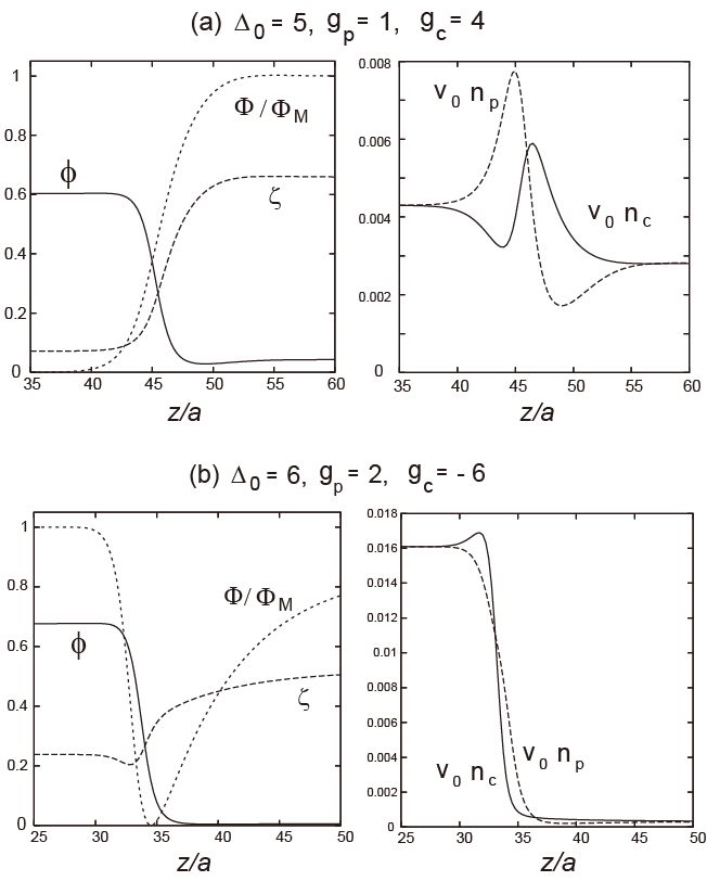
Figure 12: Interface profiles in the salt-free case for (a) $\Delta_{0}=5$, $g_{p}=1$, and $g_{c}=4$ (top) and for (b) $\Delta_{0}=8$, $g_{p}=2$, and $g_{c}=-6$ (bottom). Polymer volume fraction $\phi(z)$, normalized potential $\Phi(z)/\Phi_{M}$, and degree of ionization $\zeta(z)$ (left), and normalized charge densities $v_{0}n_{c}(z)$ and $v_{0}n_{p}(z)$ (right). The other parameters are common as $\chi=1$, $N=20$, $\nu_{M}=0.1$, $\varepsilon_{1}=-0.9\varepsilon_{0}$, and $\ell_{B}=8a/\pi$. Here $\Phi(z)$ is measured from its minimum, and $\Phi_{M}(=2.67k_{B}T/e$ in (a) and $6.86k_{B}T/e$ in (b)) is the difference of its maximum and minimum. $[$From: A. Onuki and R. Okamoto, J. Phys. Chem. B, 113, 3988 (2009).$]$

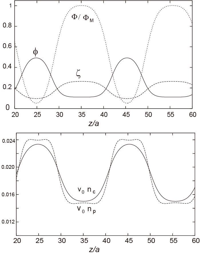
Figure 13: Periodic profiles in a salt-free mesophase with $\nu_{M}=0.5$, $\Delta_{0}=5$, $g_{p}=1$, and $g_{c}=4$. Top: $\phi(z)$. $\Phi(z)/\Phi_{M}$ with $\Phi_{M}=0.86T/e$, and $\zeta(z)$. Bottom: $v_{0}n_{c}(z)$ and $v_{0}n_{p}(z)$. $[$From: A. Onuki and R. Okamoto, J. Phys. Chem. B, 113, 3988 (2009).$]$

We give numerical results of one-dimensional profiles in equilibrium, where we set $\chi=1$, $N=20$, $\varepsilon_{1}=-0.9\varepsilon_{0}$, and $\ell_{B}=e^{2}/\varepsilon_{0}T=8a/\pi$. The dielectric constant of the solvent is 10 times larger than that of the polymer. The space will be measured in units of the molecular size $a=v_{0}^{1/3}$. In Fig.12, we show salt-free interface profiles for (a) $\Delta_{0}=5$, $g_{p}=1$, and $g_{c}=4$ and (b) $\Delta_{0}=8$, $g_{p}=2$, and $g_{c}=-6$. In the $\alpha$ and $\beta$ regions, the degree of ionization $\zeta$ is $0.071$ and $0.65$ in (a) and is $0.24$ and $0.51$ in (b), respectively. The normalized potential drop $e(\Phi_{\alpha}-\Phi_{\beta})/k_{B}T$ is $-2.67$ in (a) and $0.099$ in (b). Interestingly, in (b), $\Phi(z)$ exhibits a deep minimum at the interface position. We can see appearance of the charge density $n_{c}-n_{p}$ around the interface, resulting in an electric double layer. The counterion density is shifted to the $\beta$ region in (a) because of positive $g_{c}$ and to the $\alpha$ region in (b) because of negative $g_{c}$. The parameter $\gamma_{\rm p}$ in Eq.(6.16) is $0.75$ in (a) and $0.20$ in (b) in the $\alpha$ region, ensuring the stability of the $\alpha$ region.

The surface tension $\sigma$ is again expressed as in Eq.(3.26) with the negative electrostatic contribution. It is calculated as $\sigma=0.0175k_{B}T/a^{2}$ in (a) and as $0.0556k_{B}T/a^{2}$ in (b), while we obtain $\sigma=0.050k_{B}T/a^{2}$ without ions at the same $\chi=1$. In (a) $\sigma$ is largely decreased because the electrostatic term $\sigma_{\rm e}$ in Eq.(3.27) is increased due to the formation of a large electric double layer. In (b), on the contrary, it is increased by $10\%$ due to depletion of the charged particles from the interface OnukiPRE .

We mention calculations of the interface profiles in weakly charged polyelectrolytes in a poor solvent using self-consistent field theory Shi ; Taniguchi . In these papers, however, the solvation interaction was neglected.

6.6 Periodic states without salt. With varying the temperature (or $\chi$), the average composition $\langle{\phi}\rangle$, the amount of salt, there can emerge a number of mesophases sensitively depending on the various molecular parameters ($g_{i}$, $\Delta_{0}$, and $\nu_{M}$). In Fig.13, we show an example of a one-dimensional periodic state without salt. Here $\nu_{M}$ is set equal to $0.5$ and the charge densities are much increased. In this case, the degree of segregation and the charge heterogeneities are much milder than in the cases in Fig.12.

VII Summary and remarks

In this review, we have tried to demonstrate the crucial role of the selective solvation of a solute in phase transitions of various soft materials. We have used coarse-grained approaches to investigate mesoscopic solvation effects. Selective solvation should be relevant in understanding a wide range of mysterious phenomena in water. Particularly remarkable in polar binary mixtures are mesophase formation induced by an antagonistic salt and precipitation induced by a one-sided solute (a salt composed of hydrophilic cations and anions and a neutral hydrophobic solute). Regarding the first problem, our theory is still insufficient and cannot well explain the complicated phase behavior disclosed by the experiments Sadakane ; Seto ; SadakanePRL . To treat the second problem, we have started with the free energy density $f_{\rm tot}$ in Eq.(5.1), which looks rather obvious but yields highly nontrivial results for large $g$. Systematic experiments are now possible. In particular, this precipitation takes place on colloid surfaces as a prewetting phase transition near the precipitation curve $\chi=\chi_{\rm p}$ as in Fig.10 Okamoto .

Though still preliminary, we have also treated an ionic surfactant system, where added in water-oil are cationic surfactant, anionic counterions, and ions from a salt. In this case, we have introduced the amphiphilic interaction as well as the solvation interaction to study the interface adsorption. For ionic surfactants, the Gibbs formula Safran ; Gibbs for the surface tension is insufficient, because it neglects the electrostatic interaction.

In polyelectrolytes, the charge distributions are extremely complex around interfaces and in mesophases, sensitively depending on the molecular interaction and the dissociation process. Our continuum theory takes into account these effects in the simplest manner, though our results are still fragmentary. Salt effects in polyelectrolytes should also be further studied, on which some discussions can be found in our previous paper Onuki-Okamoto . In the future, we should examine phase separation processes in polyelectrolytes, where the composition, the ion densities, and the degree of ionization are highly inhomogeneous. In experiments, large scale heterogeneities have been observed to be pinned in space and time Ise ; Amis , giving rise to enhanced scattering at small wave numbers.

As discussed in Sec.1, there can be phase separation induced by selective hydrogen bonding. In particular, the effect of moisture uptake is dramatic in PS-PVME Hashimoto , where scattering experiments controlling the water content are desirable. To investigate such polymer blends theoretically, we may use the form in Eq.(5.1) with $n$ being the water density and $f(\phi)$ being the Flory-Huggins free energy for polymer blendsPG . Similar problems should also be encountered in block polymer systems containing ions or water. It is also known that blends of block polymer and homopolymer exhibit complicated phase behavior for different interaction parameters $\chi_{ij}$ Shi1 .

We mention two interesting effects not discussed in this review. First, there can be an intriguing interplay between the solvation and the hydrogen bonding in phase separation. For example, in some aqueous mixtures, even if they are miscible at all $T$ at atmosphere pressure without salt, addition of a small amount of a hydrophilic salt gives rise to reentrant phase separation behavior Kumar ; cluster ; Anisimov ; Misawa . On the other hand, Sadakane et al. observed a shrinkage of a closed-loop coexistence curve by adding an atagonistic salt or an ionic surfactant Seto . Second, molecular polarization of polar molecules or ions can give rise to a surface potential difference on the molecular scale at an interface. See such an example for water-hexane Patel . This effect is particularly noteworthy for hydronium ions in acid solutions Levinhyd .

We will report on the wetting transition on charged walls, rods, and colloids and the solvation-induced colloid interaction. These effects are much influenced by the ion-induced precipitation discussed in Sec.5. In these problems, first-order prewetting transitions occur from weak-to strong ionization and adsorption, as discussed in our paper on charged rods Oka . We will also report that a small amount of a hydrophobic solute can produce small bubbles in water even outside the coexistence curve, on which there have been a large number of experiments.

Acknowledgments
This work was supported by KAKENHI (Grant-in-Aid for Scientific Research) on Priority Area Soft Matter Physics from the Ministry of Education, Culture, Sports, Science and Technology of Japan. Thanks are due to informative discussions with M. Anisimov, K. Sadakane, H. Seto, T.Kanaya, K. Nishida, T. Osakai, T. Hashimoto, and F. Tanaka.

Appendix A: Statistical theory of selective solvation at small water composition

We present a simple statistical theory of binding of polar molecules to hydrophilic ions due to the ion-dipole interaction in a water-oil mixture Oka when the water volume fraction $\phi$ is small. We assume no macroscopic inhomogeneity and do not treat the large-scale electrostatic interaction. Similar arguments were given for hydrogen boning between water and polymer hydrogen1 ; hydrogen2 .

Our system has a volume $V$ and contains $N_{\rm w}$ water molecules. Using the water molecular volume $v_{0}$, we have

$$\phi=N_{\rm w}v_{0}/V=N_{\rm w}/N_{0},$$ (A1)

where $N_{0}=V/v_{0}$. We fix $N_{\rm w}$ or $\phi$ in the following. The total ion numbers are denoted by $N_{{\rm I}i}=Vn_{i}$, where $i=1$ for the cations and $i=2$ for the anions with $n_{i}$ being the average densities. The ionic volumes are assumed to be small and their volume fractions are neglected. Then the oil volume fraction is given by $1-\phi$. Each solvation shell consists of $\nu$ water molecules with $\nu=1,\cdots,Z_{i}$, where $Z_{i}$ is the maximum water number in a shell.

Let the number of the $\nu$-clusters composed of $\nu$ water molecules around an ion be $\gamma_{i\nu}N_{\rm w}$. The total number of the solvated ions is then $\gamma_{i}N_{{\rm I}i}$ with

$$\gamma_{i}=\sum_{\nu}\gamma_{i\nu}<1,$$ (A2)

where $1\leq\nu\leq Z_{i}$. The number of the bound water molecules in the $\nu$-clusters is $\nu\gamma_{i\nu}N_{{\rm I}i}$. The fraction of the unbound water molecules $\phi_{{\rm f}}$ satisfies

$$\phi_{{\rm f}}+v_{0}n_{i}\sum_{i,\nu}\nu\gamma_{i\nu}=\phi.$$ (A3)

We construct the free energy of the total system $F_{\rm tot}$ for each given set of $\gamma_{i\nu}$. In terms of the oil density $n_{\rm oil}=v_{0}^{-1}(1-\phi)$, the unbound water density $n_{\rm wf}=v_{0}^{-1}\phi_{{\rm f}}$, the unbound ion densities $n_{i{\rm f}}=n_{i}(1-\gamma_{i})$, and the cluster densities $n_{i\nu}=n_{i}\gamma_{i\nu}$, we obtain

$$\frac{F_{\rm tot}}{Vk_{B}T}=n_{\rm oil}[\ln(n_{\rm oil}\lambda_{\rm oil}^{3})-1]+n_{\rm wf}[\ln(n_{\rm wf}\lambda_{\rm w}^{3})-1]$$

$$+\sum_{i}[n_{if}\ln(n_{i{\rm f}}\lambda_{i}^{3}]-n_{i}]+\sum_{i,\nu}n_{i\nu}[\ln(n_{i\nu}\lambda_{i\nu}^{3})-w^{0}_{i\nu}]$$

$$+\chi v_{0}n_{\rm oil}n_{\rm wf}+\sum_{i,\nu}\chi_{i\nu}v_{0}n_{i\nu}n_{\rm oil},$$ (A4)

where $\lambda_{\rm oil}$, $\lambda_{\rm w}$, $\lambda_{i}$, and $\lambda_{i\nu}$ are the thermal de Broglie wavelengths, $k_{B}Tw^{0}_{i\nu}$ are the ”bare” binding free energies, and $\chi$ is the interaction parameter between the unbound water and the oil. We asssume short-range interactions among the clusters and the oil characterized by the interaction parameters $\chi_{i\nu}$ to obtain the last term. At small $\phi$, the interactions among the clusters and the unbound water are neglected. That is, we neglect the contributions of order $\phi^{2}$. We then calculate the solvation contribution $F_{\rm sol}\equiv F_{\rm tot}-F_{0}$, where $F_{0}$ is the free energy without binding ($\gamma_{i\nu}=0$). Some calculations give

$$\frac{F_{{\rm sol}}}{N_{0}k_{B}T} = \phi_{{\rm f}}(\ln\phi_{{\rm f}}-1)+\sum_{i}n_{i}(1-\gamma_{i})\ln(1-\gamma_{i})$$ (A5)

$$+\sum_{i,\nu}n_{i}\gamma_{i\nu}(\ln\gamma_{i\nu}-w_{i\nu})-\phi(\ln\phi-1),$$

where $k_{B}Tw_{i\nu}$ are the ”renormalized” binding free energies written as

$$w_{i\nu}=w^{0}_{i\nu}+3\ln(\lambda_{i}\lambda_{\rm w}^{\nu}/\lambda_{i\nu})+\nu\chi-\chi_{i\nu}.$$ (A6)

The fractions $\gamma_{i\nu}$ are determined by minimization of $F_{\rm sol}$ with respect to $\gamma_{i\nu}$ under Eqs.(A2) and (A3) as

$${\gamma_{i\nu}} = ({1-\gamma_{i}})\phi_{{\rm f}}^{\nu}e^{w_{i\nu}},$$ (A7)

$$\gamma_{i} = 1-1/(1+\sum_{\nu}\phi_{{\rm f}}^{\nu}e^{w_{i\nu}}).$$ (A8)

Substitution of Eqs.(A7) and (A8) into Eq.(A5) yields

$$\frac{F_{\rm sol}}{k_{B}TN_{0}}=\phi\ln\frac{\phi_{{\rm f}}}{\phi}+\phi-\phi_{{\rm f}}+\sum_{i}v_{0}n_{i}\ln(1-\gamma_{i}).$$ (A9)

First, we assume the dilute limit of ions $N_{I}\ll N_{\rm w}$, where we have $\phi-\phi_{{\rm f}}\ll\phi$. In the right hand side of Eq.(A9), the sum of the first three terms becomes $-(\phi-\phi_{{\rm f}})^{2}/2\phi$ and is negligible. We write ${F_{\rm sol}}$ as the sum $V\sum_{i}n_{i}\mu_{{\rm sol}}^{i}(\phi)$ and use Eq.(A8) to obtain the solvation chemical potentials of the form,

$$\mu_{{\rm sol}}^{i}(\phi)=-k_{B}T\ln(1+\sum_{\nu}\phi^{\nu}e^{w_{i\nu}}).$$ (A10)

Let the maximum of $k_{B}Tw_{i\nu}/\nu$ (per molecule for various $\nu$) be $\epsilon_{{\rm b}i}$ for each $i$ (see Eq.(2.3)). Then we obtain the expression (2.2) for the crossover volume fraction $\phi_{\rm sol}^{i}$. For $\phi>\phi_{\rm sol}^{i}$, $\gamma_{i}$ approaches unity.

Second, we consider the dilute limit of water, $\phi\ll\phi_{\rm sol}^{i}$ ($i=1,2$), where the cluster fractions $\nu_{i}$ are small and the dimers with $\nu=1$ are dominant as indicated in the experiment proton . Neglecting the contributions from the clusters with $\nu\geq 2$, we obtain

$$\gamma_{i}\cong\phi_{{\rm f}}e^{w_{i1}},\quad\phi_{{\rm f}}\cong\phi/(1+S),$$ (A11)

where $S$ is the parameter defined as

$$S=v_{0}(n_{1}e^{w_{11}}+n_{2}e^{w_{21}}).$$ (A12)

The solvation free energy behaves as

$$F_{\rm sol}/N_{0}k_{B}T\cong-\phi\ln(1+S).$$ (A13)

For $S\ll 1$, we find $\mu_{{\rm sol}}^{i}(\phi)\cong-k_{B}T\phi e^{w_{1i}}$. However, if $S\gtrsim 1$, the solvation chemical potential are not well defined.

Appendix B: Ions at liquid-liquid interface

In electrochemistry, attention has been paid to the ion distribution and the electric potential difference across a liquid-liquid interface Ham ; Hung . (In the vicinity of an air-water interface, virtually no ions are present in the bulk air region Onsager ; Levin-Flores .) Let us suppose two species of ions ($i=1,2$) with charges $Z_{1}e$ and $Z_{2}e$ ($Z_{1}>0$, $Z_{2}<0$). At low ion densities, the total ion chemical potentials $\mu_{i}$ in a mixture solvent are expressed as

$$\mu_{i}=k_{B}T\ln(n_{i}\lambda_{i}^{3})+Z_{i}e\Phi+\mu_{\rm sol}^{i}(\phi),$$ (B1)

where $\lambda_{i}$ is the thermal de Broglie length (but is an irrelevant constant in the isothermal condition) and $\Phi$ is the local electric potential. This quantity is a constant in equilibrium. For neutral hydrophobic particles the electrostatic term is nonexistent, so we have Eq.(2.5).

We consider a liquid-liquid interface between a polar (water-rich) phase $\alpha$ and a less polar (oil-rich) phase $\beta$ with bulk compositions $\phi_{\alpha}$ and $\phi_{\beta}$ with $\phi_{\alpha}>\phi_{\beta}$. The bulk ion densities far from the interface are written as $n_{i\alpha}$ in phase $\alpha$ and $n_{i\beta}$ in phase $\beta$. From the charge neutrality condition in the bulk regions, we require

$$Z_{1}n_{1\alpha}+Z_{2}n_{2\alpha}=0,\quad Z_{1}n_{1\beta}+Z_{2}n_{2\beta}=0.$$ (B2)

The potential $\Phi$ tends to constants $\Phi_{\alpha}$ and $\Phi_{\beta}$ in the bulk two phases, yielding a Galvani potential difference, $\Delta\Phi=\Phi_{\alpha}-\Phi_{\beta}.$ Here $\Phi$ approaches its limits on the scale of the Debye screening lengths, $\kappa_{\alpha}^{-1}$ and $\kappa_{\beta}^{-1}$, away from the interface, so we assume that the system extends longer than $\kappa_{\alpha}^{-1}$ in phase $\alpha$ and $\kappa_{\beta}^{-1}$ in phase $\beta$. Here we neglect molecular polarization of solvent molecules and surfactant molecules at an interface (see comments in the summary section).

The solvation chemical potentials $\mu_{\rm sol}^{i}(\phi)$ also take different values in the two phases due to their composition dependence. So we define the differences $\Delta\mu_{\alpha\beta}^{i}$ as in Eq.(2.4). The continuity of $\mu_{i}$ across the interface gives

$$k_{B}T\ln(n_{i\alpha}/n_{i\beta})+Z_{i}e\Delta\Phi-\Delta\mu_{\alpha\beta}^{i}=0,$$ (B3)

where $i=1,2$. From Eqs.(B2) and (B3), the Galvani potential difference $\Delta\Phi$ is expressed as Hung ; OnukiPRE

$$\Delta\Phi=[{\Delta\mu_{\alpha\beta}^{1}-\Delta\mu_{\alpha\beta}^{2}}]/{e(Z_{1}+|Z_{2}|)}.$$ (B4)

Similar potential differences also appear at liquid-solid interfaces (electrodes) Ham . The ion densities in the bulk two phases (in the dilute limit) are simply related by

$$\frac{n_{1\beta}}{n_{1\alpha}}=\frac{n_{2\beta}}{n_{2\alpha}}=\exp\bigg{[}-\frac{|Z_{2}|{\Delta\mu_{\alpha\beta}^{1}}+Z_{1}\Delta\mu_{\alpha\beta}^{2}}{(Z_{1}+|Z_{2}|)k_{B}T}\bigg{]}.$$ (B5)

However, if three ion species are present, the ion partitioning between two phases is much more complicated OnukiJCP .

References

• (1) Y. Levin, Rep. Prog. Phys. 65, (2002) 1577.
• (2) J.L. Barrat and J.F. Joanny, Adv. Chem. Phys. XCIV, I. Prigogine, S.A. Rice Eds., John Wiley $\&$ Sons, New York 1996.
• (3) C. Holm, J. F. Joanny, K. Kremer, R. R. Netz, P. Reineker, C. Seidel, T. A. Vilgis, and R. G. Winkler, Adv. Polym. Sci. 166, 67 (2004).
• (4) A.V. Dobrynin and M. Rubinstein, Prog. Polym. Sci. 30, 1049 (2005).
• (5) P.G. de Gennes, Scaling Concepts in Polymer Physics (Ithaca, Cornell Univ. Press) 1980.
• (6) S.A. Safran, Statistical Thermodynamics of Surfaces, Interfaces, and Membranes (Westview Press, 2003).
• (7) J. N. Israelachvili, Intermolecular and Surface Forces (Academic Press, London, 1991).
• (8) Y. Marcus, Ion Solvation (Wiley, New York, 1985).
• (9) V. Gutmann, The Donor-Acceptor Approach to Molecular Interactions (Plenum, New York, 1978).
• (10) D. Chandler, Nature 437, 640 (2005).
• (11) E.L. Eckfeldt and W.W. Lucasse, J. Phys. Chem. 47, 164 (1943); B.J. Hales, G.L. Bertrand, and L.G. Hepler, J. Phys. Chem. 70, 3970 (1966).
• (12) V. Balevicius and H. Fuess, Phys. Chem. Chem. Phys. 1 ,1507 (1999).
• (13) T. Narayanan and A. Kumar, Phys. Rep. 249, 135 (1994).
• (14) J. Jacob, A. Kumar, S. Asokan, D. Sen, R. Chitra, and S. Mazumder, Chem. Phys. Lett. 304, 180 (1999).
• (15) M. Misawa, K. Yoshida, K. Maruyama, H. Munemura, and Y. Hosokawa, J. of Phys. and Chem. of Solids 60, 1301(1999).
• (16) M. A. Anisimov, J. Jacob, A. Kumar, V. A. Agayan, and J. V. Sengers, Phys. Rev. Lett. 85, 2336 (2000).
• (17) T. Takamuku, A. Yamaguchi, D. Matsuo, M. Tabata, M. Kumamoto,J. Nishimoto, K. Yoshida, T. Yamaguchi, M. Nagao, T. Otomo, and T. Adachi, J. Phys. Chem. B 105, 6236 (2001).
• (18) T. Arakawa and S. N. Timasheff, Biochemistry, 23, 5912 (1984).
• (19) S. N. Timasheff, PNAS, 99, 9721 (2002).
• (20) V. M. Nabutovskii, N. A. Nemov, and Yu. G. Peisakhovich, Phys. Lett. 79A, 98 (1980).
• (21) V. M. Nabutovskii, N. A. Nemov, and Yu. G. Peisakhovich, Mol. Phys. 54, 979 (1985).
• (22) A. Onuki and H. Kitamura, J. Chem. Phys., 121, 3143 (2004).
• (23) A. Onuki, Phys. Rev. E 73 021506, (2006).
• (24) A. Onuki, J. Chem. Phys. 128, 224704 (2008).
• (25) G. Marcus, S. Samin, and Y. Tsori, J. Chem. Phys. 129, 061101 (2008).
• (26) M. Bier, J. Zwanikken, and R. van Roij, Phys. Rev. Lett. 101, 046104 (2008).
• (27) J. Zwanikken, J. de Graaf, M. Bier, and R. van Roij, J. Phys.: Condens. Matter 20, 494238 (2008).
• (28) D. Ben-Yaakov, D. Andelman, D. Harries, and R. Podgornik, J. Phys. Chem. B 10, 6001(2009).
• (29) T. Araki and A. Onuki, J. Phys.: Condens. Matter 21, 424116 (2009).
• (30) A. Onuki, T. Araki, and R. Okamoto, to be published in J. Phys.: Condens. Matter.
• (31) B. Rotenberg, I. Pagonabarragac, and D. Frenkel, Faraday Discuss., 144, 223 (2010).
• (32) R. Okamoto and A. Onuki, Phys. Rev. E 82, 051501 (2010).
• (33) A. Onuki and R. Okamoto, J. Phys. Chem. B, 113, 3988 (2009).
• (34) R. Okamoto and A. Onuki, J. Chem. Phys. 131, 094905 (2009).
• (35) A. Onuki, Europhys. Lett. 82, 58002 (2008).
• (36) A. Onuki, Phase Transition Dynamics (Cambridge University Press, Cambridge, 2002).
• (37) J. D. Reid, O. R. Melroy, and R. P. Buck, J. Electroanal. Chem. Interfacial Electrochem. 147, 71 (1983).
• (38) G. Luo, S. Malkova, J. Yoon, D. G. Schultz, B. Lin, M. Meron, I. Benjamin, P. Vanysek, and M. L. Schlossman, Science 311, 216 (2006).
• (39) K. Sadakane, H. Seto, H. Endo, and M. Shibayama, J. Phys. Soc. Jpn., 76, 113602 (2007).
• (40) K. Sadakane, N. Iguchi, M. Nagao, H. Endo, Y. B. Melnichenko, and Hideki Seto, Soft Matter, 7, 1334 (2011).
• (41) K. Sadakane,, A. Onuki, K. Nishida, S. Koizumi, and H. Seto, Phys. Rev. Lett. 103, 167803 (2009).
• (42) K. Aoki, M. Li, J. Chen, and T. Nishiumi Electrochem. Commun. 11, 239 (2009).
• (43) K. Wojciechowski and M. Kucharek, J. Phys. Chem. B, 113, 13457 (2009).
• (44) G. W. Euliss and C. M. Sorensen, J. Chem. Phys. 80, 4767 (1984).
• (45) Y. Georgalis, A. M. Kierzek, and W. Saenger, J. Phys. Chem. B 2000, 104, 3405.
• (46) A. F. Kostko, M. A. Anisimov, and J. V. Sengers, Phys. Rev. E 70, 026118 (2004).
• (47) M. Wagner, O. Stanga, and W. Schr$\ddot{\rm o}$er, Phys. Chem. Chem. Phys. 6, 580 (2004).
• (48) C. Yang, W. Li, and C. Wu, J. Phys. Chem. B 108, 11866 (2004).
• (49) M. Sedlak, J. Phys. Chem. B 110, 4329, 4339, 13976 (2006).
• (50) F. Jin, J. Ye, L. Hong, H. Lam, and C. Wu, J. Phys. Chem. B 111, 2255 (2007).
• (51) J. Jacob, M. A. Anisimov, J. V. Sengers, A. Oleinikova, H. Weing$\ddot{\rm a}$rtner, and A. Kumar, Phys. Chem. Chem. Phys. 3, 829 (2001).
• (52) G. R. Anderson and J. C. Wheeler, J. Chem. Phys. 69, 2082 (1978).
• (53) R. E. Goldstein, J. Chem. Phys. 80, 5340 (1984).
• (54) A. Matsuyama and F. Tanaka, Phys. Rev. Lett. 65, 341 (1990).
• (55) S. Bekiranov, R. Bruinsma, and P. Pincus, Phys. Rev. E 55, 577 (1997).
• (56) J.L. Tveekrem and D.T. Jacobs, Phys. Rev. A 27, 2773 (1983).
• (57) D. Beaglehole, J. Phys. Chem. 87, 4749 (1983).
• (58) T. Hashimoto, M. Itakura, and N. Shimidzu, J. Chem. Phys. 85, 6773-6786 (1986).
• (59) P.G. de Gennes P. G. and C. Taupin, J. Phys. Chem. 86, 2294 (1982).
• (60) E. Raphael and J. F. Joanny, Europhys. Lett. 13, 623 (1990).
• (61) I. Borukhov, D. Andelman, and H. Orland, Europhys. Lett.32, 499 (1995).
• (62) I. Borukhov, D. Andelman, R. Borrega, M. Cloitre, L. Leibler, and H. Orland, J. Phys. Chem. B 104, 11027 (2000).
• (63) P. G. Arscott, C. Ma, J. R. Wenner and V. A. Bloomfield, Biopolymers, 36, 345 (1995).
• (64) A. Hultgren and D. C. Rau, Biochemistry 43, 8272 (2004).
• (65) C. Stanley and D. C. Rauy, Biophy. J. 91, 912 (2006).
• (66) J.W. Gibbs, Collected Works, Vol. 1 (Yale University Press, New Haven, CT) 1957, pp. 219-331.
• (67) D. N. Shin, J. W. Wijnen, J. B. F. N. Engberts, and A. Wakisaka, J. Phys. Chem. B 106, 6014 (2002).
• (68) A. Wakisaka, S. Mochizuki, and H. Kobara, J. of Sol. Chem. 33, 721(2004).
• (69) T. Osakai and K. Ebina, J. Phys. Chem. B 102, 5691 (1998).
• (70) T. Osakai, M. Hoshino, M. Izumi, M. Kawakami, and K. Akasaka, J. Phys. Chem. B 104, 12021 (2000).
• (71) S. Garde, G. Hummer, A. E. Garcia, M. E. Paulaitis, and L. R. Pratt, Phys. Rev. Lett. 77, 4966 (1996).
• (72) P. R. ten Wolde and D. Chandler, PNAS 99, 6539 (2002).
• (73) M. Born, Z. Phys. 1, 45 (1920).
• (74) Y. Marcus, Chem. Rev. 88, 1475 (1988).
• (75) A. Hamnett, C. H. Hamann, and W. Vielstich, Electrochemistry (Wiley-VCH, Weinheim, 1998).
• (76) Le Quoc Hung, J. Electroanal. Chem. 115, 159 (1980); ibid. 149, 1 (1983).
• (77) J. Koryta, Electrochim. Acta 29, 445 (1984).
• (78) A. Sabela, V. Marecek, Z. Samec, and R. Fuocot, Electrochim.Acta, 37, 231 (1992).
• (79) L. Degr$\rm\grave{e}$ve and F.M. Mazz$\rm{\acute{e}}$, Molecular Phys. 101, 1443 (2003).
• (80) A.A. Chen and R.V. Pappu, J. Phys. Chem. B 111, 6469 (2007).
• (81) L. Onsager and N. N. T. Samaras, J. Chem. Phys. 2, 528 (1934).
• (82) Y. Levin and J. E. Flores-Mena, Europhys. Lett. 56, 187 (2001).
• (83) P. Debye and K. Kleboth, J. Chem. Phys. 42, 3155 (1965).
• (84) K. Tojo, A. Furukawa, T. Araki, and A. Onuki, Eur. Phys. J. E 30 (2009) 55-64.
• (85) A. A. Aerov, A. R. Khokhlov, and I. I. Potemkin, J. Phys. Chem. B 111, 3462 (2007); ibid. 111, 10189 (2007).
• (86) B.L. Bhargava and M. L. Klein, Molecular Physics, 107, 393 (2009).
• (87) P.G. de Gennes, Le Journal de Physique-Lettre 37, 59(1976).
• (88) K. Weissenborn and R. J. Pugh, J. Colloid Interface Sci. bf 184, 550 (1996).
• (89) A. P. dos Santos and Y. Levin, J. Chem. Phys. 133, 154107 (2010).
• (90) A. L. Nicols and L. R. Pratt, J. Chem. Phys. 80, 6225 (1984).
• (91) G. Jones and W. A. Ray, J. Am. Chem. Soc. 59, 187 (1937); ibid. 63, 288 (1941); ibid. 63, 3262 (1941).
• (92) M. Seul and D. Andelman, Science 267, 476 (1995).
• (93) V. Yu. Borye and I. Ya. Erukhimovich, Macromolecules 21, 3240 (1988).
• (94) J. F. Joanny and L. Leibler, J. Phys. (France) 51, 547 (1990).
• (95) O. Braun, F. Boue, and F. Candau, Eur. Phys. J. E 7, 141 (2002).
• (96) I.F. Hakim and J. Lal, Europhys. Lett. 64, 204 (2003).
• (97) I.F. Hakim, J. Lal, and M. Bockstaller, Macromolecules 37, 8431 (2004).
• (98) Shi, A.-C.; Noolandi, J. Maromol. Theory Simul. 1999, 8(3), 214.
• (99) Q. Wang, T. Taniguchi, and G.H. Fredrickson, J. Phys. Chem B 2004, 108, 6733-6744; ibid. 2005, 109, 9855-9856.
• (100) N. Ise, T. Okubo, S. Kunugi, H. Matsuoka, K. Yamamoto, and Y. Ishii, J. Chem. Phys. bf 81, 3294 (1984).
• (101) B.D. Ermi and E. J. Amis, Macromolecules 31, 7378 (1998).
• (102) J. Zhou and An-Chang Shi, J. Chem. Phys. 130, 234904 (2009).
• (103) S.A. Patel and C.L. Brooks III, J. Chem. Phys. 124, 204706 (2006).