Experimental realization of mixed-synchronization in counter-rotating coupled oscillators
Abstract
Recently, a novel mixed–synchronization phenomenon is observed in counter–rotating nonlinear coupled oscillators r0 . In mixed–synchronization state: some variables are synchronized in–phase, while others are out–of–phase. We have experimentally verified the occurrence of mixed–synchronization states in coupled counter–rotating chaotic piecewise oscillator. Analytical discussion on approximate stability analysis and numerical confirmation on the experimentally observed behavior is also given.
pacs:
05.45.XtI Introduction
Huygens first describes the anti–phase synchronization in a pair of pendulum clocks ch . Later, the idea of synchronization of two identical chaotic system was introduced by Pecora and Carroll r1 . Synchronization of chaotic systems has attracted much attention due to its potential application in secure communication, chemical and biological system, information science, and so on r1a . Many different synchronization states have been studied in literature, namely complete or identical synchronization (CS) r1 ; r3 ; r4 , in–phase (PS) r6 ; r7 , anti–phase r8 , lag synchronization (LS) r9 , generalized synchronization (GS) r10 ; r11 , intermittent lag synchronization(ILS) r12 ; r13 , and anti-synchronization (AS) r14 ; r15 ; r16 in which one of the dynamical variable is synchronized then rest of variable follow the same. All these type of synchronization can be achieved with various type of interactions e.g. mismatch oscillators r17 , conjugate r19 ; r19a , delay r18 , and nonlinear r20 ; r20a , indirect raa ; amit .
If the directions of rotation of two oscillators are same, the system is co–rotating, while system of oscillators rotating in opposite direction is called counter–rotating. Coupled co–rotating nonlinear oscillators have been extensively studied from both theoretical and experimental point of view r1a . Recently, a mixed–synchronization phenomenon was observed in coupled counter–rotating nonlinear oscillators r0 , similar phenomena was engineered using a general formulation of coupling function in co–rotating coupled oscillators r26 ; r26a . In mixed–synchronization state, some variables are synchronized to in–phase state while other variables are out–of–phase. The mixed–synchronization phenomenon is also studied in the case of extended systems r0 .
In this Letter, we present the experimental observation of the mixed–synchronization in two diffusive coupled counter–rotating chaotic piecewise oscillators. The analytical discussion on approximate stability analysis and numerical simulations are in close agreement with experimental results. The critical value of coupling strength, where counter–rotating coupled chaotic oscillators are synchronized, is larger in experiments as compared to numerical simulations because of parameter mismatch in circuit implementation.
The Letter is organized as follows: In the section II we numerically study the mixed–synchronization phenomenon in the coupled chaotic oscillators for piecewise system. The linear stability analysis and numerical results are presented. The experimental setup and the results of coupled counter–rotating chaotic oscillators are discussed in section III. Concluding remarks and discussion about the mixed–synchronization in coupled counter–rotating chaotic oscillators are given in section IV.
II The model system
Here, we illustrate the mixed–synchronization phenomena in two diffusive coupled piecewise r23 systems given by following equations
| (1) |
Here, in functions and , ’s represents the internal frequency of two oscillators with opposite sign and it depends on the parameters and . The function if , or if . The rotation of Piecewise system (in plane) can be changed by changing the sign of and . The first system has counter clockwise rotation while second has clockwise rotation. The parameters values are: , , , , , , and . The coupling parameter is . For identical oscillators, .
The fixed points of the piecewise oscillators are , where depends on the sign of the and . The change in the dynamical behavior arises from the coupling between two identical piecewise oscillators.
II.1 Numerical Results
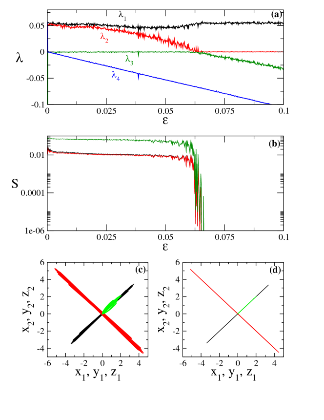
We numerically study the mixed–synchronization of two coupled counter–rotating piecewise oscillators. At the very small coupling strength the two oscillators are uncorrelated. As the coupling strength increases, the phase synchronization set in when forth largest Lyapunov exponent becomes negative and complete synchronization occurs when third largest Lyapunov exponent becomes negative as shown in Fig. 1(a).
To quantify synchronization, we use the following similarity function defined with respect to dynamical variables, and , of the chaotic oscillator r9
| (2) |
| (3) |
Synchronization (complete and anti) is characterized by for and variables respectively. The variables and are in–phase while and are out–of–phase. The two variables and shows complete in–phase and out–of–phase synchronization respectively for coupling strength , where . The variable of the system also goes to complete synchronization state, where is defined similar to . The in–phase synchronization in and while out–of–phase in and is shown in Figure 1(c). The complete synchronization in and with zero relative phase while out–of–phase state of and with phase difference of is shown in Figure 1(d).
II.2 Linear Stability Analysis
We analyze the stability of the mixed–synchronized state of two counter–rotating coupled chaotic systems given by Eq. (1) in plane. The method of approximate linear stability analysis is adopted for synchronization criteria raa . If and represent the deviation of coordinates and respectively from the synchronization state, their dynamic is governed by the linearized equation as
| (4) |
Where the and are functions in terms of coordinate and parameter. , i=1,2 represent the frequency of the oscillators. The criteria for the stability is that synchronization state corresponding to fixed point will be stable if all eigen values of the Eqs. (4) are negative.
Dynamics of the deviation from the synchronization state is governed by the linearized equation of Eqs (1).
| (5) |
Where , and are parameters. For the Perfect synchronization in counter rotating coupled system , i.e. (complete) and (Anti-synchronization), we can define
| (6) |
Then Eqs (5) can be written as
| (7) |
If we assume that the time average values of Jacobian matrix elements and , where i=1,2 are approximately the same and can be replaced by an effective constant value and .
In the case of counter rotating systems, frequency of the coupled systems are of opposite sign: and . Then
| (8) |
Eliminating from above equations, we get
| (9) |
Solution of the equation , we get
| (10) |
The synchronization state define by and , is stable if Re[m] is negative for both the solutions.
-
•
If , m is complex and the stability condition becomes .
-
•
If , m real and the stability condition becomes .
The transition to stable synchronization is given by the threshold values of the parameters satisfying the condition
| (11) |
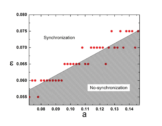
Figure 2 shows the transition from the unsynchronized to mixed–synchronization state in the space. A linear relations is clearly seen and the solid line is drawn with the effective and , thus validating the transition criterion of Eq. (11) obtained from the stability theory. The condition given by Eq. (11) is necessary but not sufficient for synchronization.
III Experimental Setup and Results
Experiments are conducted using a pair of electronic oscillators whose dynamics mimic that of the chaotic oscillator r23 . One of the oscillators rotate clockwise while another anti–clockwise. The two oscillators are approximately identical since in reality it is not possible to ensure that parameters are exactly equal. Further, unlike the piecewise system (Eq. (1)) discussed above, the coupling is asymmetric and frequencies of the oscillators are not equal in experiment. Hence, we observe lag and phase synchronization in coupled piecewise oscillators as coupling is increased.
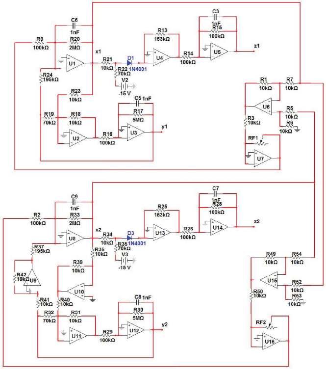
The Piecewise oscillator circuit shows the dynamics of rotation in counter clockwise. We have to connect two inverting amplifier and (as shown in Fig. 3) for changing the direction of the rotation in circuit. Both piecewise oscillators are consisting of the passive components like resistance , capacitors , diodes and operational amplifier uA741 . We use simple linear scheme for the coupling between variables of the two piecewise oscillators. The OPAMP in circuit are used for linear coupling scheme. and are the variable resistors characterizing the coupling parameter. The electronic components in circuits are carefully chosen and values are mentioned in the diagram (Fig. 3). The typical oscillating frequencies of the circuits are in the audio frequency range. Both oscillators are operated by a low-ripple and low noise power supply. The output voltages form both oscillators are monitored using digital oscilloscope 100MHz 2 channel (Agilent DSO1012A) with maximum sampling rate of 2 GSa/s.
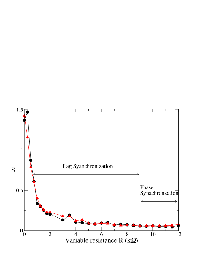
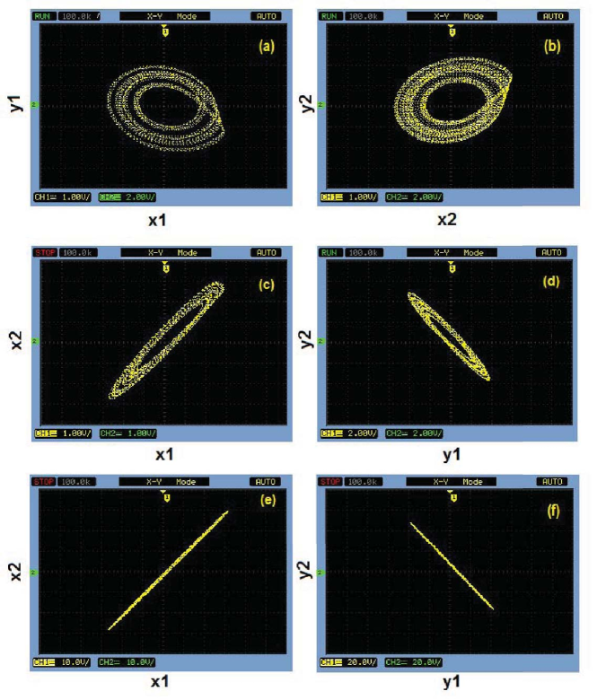
Transitions from asynchronous chaos to lag synchronization and then to in–phase synchronization is observed at the critical values of variable resistance, and , respectively. The lag synchronization occurs in the interval [, ], where = 0.5k and = 9k. It has been observed in experiments that the variables of one of the oscillator tends to fellow the variables of the another oscillator in some range of the coupling strength A21 . Here, it is due to the parameter mismatch in the coupled oscillators. The Similarity function of and variables (Eq. (2) and (3)) of the coupled piecewise oscillator with variable resistance is shown in Fig. 4. At = = 1.4k the output voltage of and shows in–phase dynamics while and are out–of–phase. Phase relationship of and variables with lag synchronization are shown in Fig. 5(c-d). Further increase of the coupling strength shows the transition from lag to phase synchronization. Phase relationship at = = 11.2k is shown in Fig. 5(e-f).
IV Conclusion
We presented the experimental evidence of mixed–synchronization in the piecewise oscillators circuit via diffusive type of coupling under the parameter mismatch. The experimental results are in close agreement with the numerical results. The critical value of coupling strength for onset of mixed–synchronization is calculated using approximate linear stability analysis. We have also studied the sprott circuit r24 and obtained similar results for mixed-synchronization. The natural emergence of novel mixed–synchronization phenomenon in chaotic as well as limit cycle counter–rotating coupled oscillators has possible applications in secure communication and chaos based computing.
Acknowledgments
We thank Awadhesh Prasad and Syamal Kumar Dana for useful discussion and critical comments on the manuscript. We would like to acknowledge the financial support from DST, India and LNMIIT, Jaipur.
References
- (1) A. Prasad, Chaos, Solitons and Fractals, 43, (2010) 42.
- (2) C. Huygens, C. Horoloqium Oscilatorium, (Apud F. Muquet, Parisiis, 1673); English translation: The pendulum clock , (Iowa State University Press, Ames).
- (3) L. M. Pecora, T. L. Carroll, Phys. Rev. Lett. 64 (1990) 821.
- (4) A. S. Pikovsky, M. G. Rosenblum, J. Kurths, Synchronization: A Universal Concept in Nonlinear Sciences, (Cambridge Nonlinear Science Series) Cambridge University Press, Cambridge, 2001.
- (5) H. Fujisaka, T. Yamada, Prog. Theor. Phys. 69, (1983) 32.
- (6) V. S. Afraimovich, N. N. Verichev, M. I. Rabinovich, Izvestiya Vysshikh Uchebnykh Zavedenii Radiofizika, Biom. J. 29, (1986) 1050.
- (7) M. G. Rosenblum, A. S. Pikovsky, J. Kurths, Phys. Rev. Lett. 76 (1996) 1804.
- (8) E. R. Rosa, E. Ott, M. H. Hess, Phys. Rev. Lett. 80 (1998) 1642.
- (9) J. Liu, C. Ye, S. Zhang, W. Song, Phys. Lett. A 274 (2000) 27.
- (10) M. G. Rosenblum, A. S. Pikovsky, J. Kurths, Phys. Rev. Lett. 78 (1997) 4193.
- (11) N. F. Rulkov, M. M. Sushchik, L. S. Tsimring, H. D. I. Abarbanel, Phys. Rev. E 51 (1995) 980.
- (12) L. Kocarev, U. Parlitz, Phys. Rev. Lett. 76 (1996) 1816.
- (13) S. Boccaletti, D. L. Valladares, Phys. Rev. E 62 (2000) 7497.
- (14) M. A. Zaks, E. H. Park, M. G. Rosenblum, J. Kurths, Phys. Rev. Lett. 82 (1999) 4228.
- (15) S. Sivaprakasam, I. Pierce, P. Rees, P. S. Spencer, K. A. Shore and A. Valle, Phys. Rev. A 64 (2001) 013805.
- (16) C. M. Kim, S. Rim, W. H. Kye, J. W. Ryu, Y. J. Park, Phys. Rev. A 320 (2003) 39.
- (17) H. Zhu, and B. Cui, CHAOS, 17 (2007) 043122.
- (18) D. G. Aronson, G. B. Ermentrout, N. Kopell, Physica D 41 (1990) 403.
- (19) R. Karnatak, R. Ramaswamy, A. Prasad, Phys. Rev. E 76 (2007) 035201.
- (20) R. Karnatak, R. Ramaswamy, A. Prasad, CHAOS, 19 (2009) 033143.
- (21) D. V. Ramana Reddy, A. Sen, G. L. johnston, Phys. Rev. Lett. 80 (1998) 15109.
- (22) A. Prasad, M. Dhamala, B. M. Adhikari, R. Ramaswamy, Phys. Rev. E 81 (2010) 027201.
- (23) A. Prasad, M. Dhamala, B. M. Adhikari, R. Ramaswamy, Phys. Rev. E 82 (2010) 027201.
- (24) V. Resmi, G. Ambika, and R. E. Amritkar, Phys. Rev. E 81 (2010) 046216.
- (25) A. Sharma and M. D. Shrimali, Pramana - Journal of Physics, in–press (2011).
- (26) I. Grosu, R. Banerjee, P. K. Roy, and S. K. Dana, Phys. Rev. E 76 (2007) 035201.
- (27) S. K. Dana, E. Padmanaban, R. Banerjee, P. K. Roy, I. Grosu, International Symposium on Signals, Circuits and Systems, 2009.
- (28) J. F. Heagy, T. L. Corroll, L. M. Pecora, Phys. Rev. E 50 (1994) 3.
- (29) S. Taherion, Y. C. Lai, Phys. Rev. E 59 (1999) 6248.
- (30) J. C. Sprott, Phys. Lett. A 266 (2000) 19.
Figure Captions
Figure 1: (Color online) (a) The largest four Lyapunov exponents of identical coupled counter–rotating piecewise oscillators. (b) the similarity functions for and variables of the coupled oscillators. (c) and (d) the phase relationship between the variables and at and respectively.
The similarity function and dynamics for variables , and are marked by black, red, and green color respectively.
Figure 2: (Color online) Transition from unsynchronized to mixed–synchronized region is shown in the parameter plane for coupled piecewise oscillators.
Figure 3: (Color online) Schematic diagram of two bidirectional coupled (counter clockwise and clockwise) piecewise chaotic oscillator.
Variable resistors are used to change the coupling. The OPAMP are type of uA741. All resistors are metal film type with tolerance and capacitors are polyester type with tolerance . The circuit is run by source.
Figure 4: (Color online) Similarity function for (circle) and (triangle) variables of the experimental system of two coupled counter rotating piecewise oscillators with variable resistance .
Figure 5: (Color online) Dynamic of the piecewise oscillator in (a) counter clockwise rotation (b) clockwise rotation. The phase relationship of and variables respectively at for lag–synchronization in (c) and (d). mixed–synchronization at in (e) and (f).