Regimes of strong light-matter coupling under incoherent excitation

Abstract

We study a two-level system (atom, superconducting qubit or quantum dot) strongly coupled to the single photonic mode of a cavity, in the presence of incoherent pumping and including detuning and dephasing. This system displays a striking quantum to classical transition. On the grounds of several approximations that reproduce to various degrees exact results obtained numerically, we separate five regimes of operations, that we term “linear”, “quantum”, “lasing”, “quenching” and “thermal”. In the fully quantized picture, the lasing regime arises as a condensation of dressed states and manifests itself as a Mollow triplet structure in the direct emitter photoluminescence spectrum, which embeds fundamental features of the full-field quantization description of light-matter interactions.

I Introduction

The strong coupling regime is the ultimate limit of light-matter interaction, at the level of a single quantum or a few quanta of excitations. This gave rise to the field of cavity Quantum Electrodynamics (cavity QED) Haroche and Raimond (2006), which in the recent years has blossomed in a large variety of physical systems, from atoms Raimond et al. (2001) to semiconductors Khitrova et al. (2006) passing by superconducting circuits Makhlin et al. (2001) and nanomechanical oscillators Kippenberg (2008). A fascinating aspect of this fundamental problem is how it bridges the gap between quantum and classical coherence. In the former case, one has quantum superpositions of light and matter, entangling photons with the ground and excited states of the emitter. In the latter case, one has a classical photon field, a continuous function of a continuous variable, fully specified in all its attributes. The passage from one to the other can be tracked in the one-atom lasing transition. The one-atom laser is a concept first proposed and theoretically studied by Mu and Savage Mu and Savage (1992), with the aim of achieving lower thresholds for lasing. They encouraged experimentalists to bring the number of atoms $N$ in a conventional laser to unity. In a very high quality factor cavity, the emitter reaches the strong coupling regime at the single excitation level. They showed that in this regime, a single incoherently excited emitter (a two level system in the simplest case) can constitute the whole gain medium and populate singlehandedly the cavity with a very large number of photons. If the spontaneous emission rate of the atom into other modes than the cavity is small, the growth in the population of photons exhibits no threshold as a function of the pumping rate P. R. Rice (1994) and develops a classical (Poissonian) field statistics, thanks to the efficient periodic exchange of excitations with the atom.

On the theoretical side, the single-atom laser has been extensively studied for its qualities as a laser Mu and Savage (1992); Ginzel et al. (1993); Löffler et al. (1997); Jones et al. (1999); Benson and Yamamoto (1999); Karlovich and Kilin (2001); Kilin and Karlovich (2002); Clemens et al. (2004); Karlovich and Kilin (2008); del Valle et al. (2009); Poddubny et al. (2010); Gonzalez-Tudela et al. (2010); Ritter et al. (2010); Auffèves et al. (2010); del Valle and Laussy (2010); Gartner (2011), mostly solving its steady state numerically but also through analytical techniques, such as the continued fraction expansion Gartner (2011) or phase-space representation Karlovich and Kilin (2001); Kilin and Karlovich (2002); Gartner (2011), and under different approximations such as the few-photon Löffler et al. (1997); Karlovich and Kilin (2008); Auffèves et al. (2010); Gartner (2011) or semiclassical Mu and Savage (1992); Benson and Yamamoto (1999); Poddubny et al. (2010); del Valle and Laussy (2010); Gartner (2011) dynamics. On the other hand, the spectral properties, that is, atom and cavity photoluminescence emission spectra, have been studied only numerically Mu and Savage (1992); Ginzel et al. (1993); Löffler et al. (1997); Benson and Yamamoto (1999); Clemens et al. (2004); del Valle et al. (2009); Poddubny et al. (2010), although some approximations for the linewidth of the cavity spectrum, that converges to a single peak and exhibits the standard line-narrowing, provided useful analytical expressions Benson and Yamamoto (1999); Poddubny et al. (2010). Given that the cavity field is coherent in the lasing regime, the back-action of the field on the emitter leads to the formation of a Mollow triplet in its spontaneous emission spectrum Löffler et al. (1997); Clemens et al. (2004); del Valle et al. (2009), with similar properties to that theoretically predicted by Mollow for an atom under resonant laser excitation Mollow (1969). This structure is of a great fundamental interest as it represents a pinnacle of nonlinear quantum optics.

On the experimental side, the strong coupling regime is now firmly established at the single and few photon level with atoms Boca et al. (2004) as well as with artificial atoms, superconducting qubits Wallraff et al. (2004); Fink et al. (2008) or semiconductor quantum dots Reithmaier et al. (2004); Yoshie et al. (2004); Peter et al. (2005), and the one atom laser as described above has been realised in all these systems McKeever et al. (2003); Astafiev et al. (2007); Nomura et al. (2010). The Mollow triplet under incoherent pumping has not yet been reported in any experiment, one reason being that they typically focus on the cavity field lasing properties. Only the original configuration proposed by Mollow, under resonant coherent excitation, has been reported, also in all the systems above, namely with a single atom Wu et al. (1975), a molecule Wrigge et al. (2008), a superconducting qubit Astafiev et al. (2010) and a quantum dot Muller et al. (2007); Vamivakas et al. (2009); Flagg et al. (2009); Ates et al. (2009).

In this text, we consider in detail the quantum to classical transition that leads to lasing in strong-coupling, starting from the fully quantized description of Jaynes and Cummings Jaynes and Cummings (1963). We show that quantization breaks down as coherence is formed and a classical description becomes more appropriate. We provide several limiting cases that describe the system in its various regimes of operation. Varying degrees of agreement are afforded depending on the complexity of the approximation. We provide compact analytical approximations in the simplest cases and a straightforward numerical procedure that leads to an excellent quantitative agreement. We include pure dephasing, important in solid state systems Ulrich et al. (2011); Roy and Hughes (2011), and arbitrary detuning between the modes. We focus more particularly on the lasing regime at resonance, where we show that the emergence of a Mollow triplet manifests classical nonlinearities of strong light-matter coupling in cavity-QED. As a whole, we show that the lasing transition is a rich and complex one and we hope to give a rather comprehensive view of its various limits.

The remaining of this text is organized as follows. As the most striking and characteristic manifestation of lasing in strong coupling is the Mollow triplet formed under incoherent pumping, we first revisit its coherent excitation counterpart, this is done in Sec. II, extending it to include pure dephasing and detuning. Starting from Sec. III, we turn to the case of incoherent excitation exclusively and obtain analytically the steady state, mode populations and photon counting statistics (III.1), the system full density matrix (III.2) and the two-time correlators needed to compute the power (or luminescence) spectra (III.3). We derive the expressions for the lasing properties by applying the semiclassical approximation that we compare to other approximations that describe the transition into and out-of lasing. In Sec. IV, we put all these elements together and derive the spectra of emission for both the cavity and the emitter. We analyse the resonances of the system (IV.2) as well as the elastic scattering component (IV.3). We apply again the semiclassical approximation to simplify the emitter spectra into a compact closed-form expression for the Mollow triplet under incoherent pumping (IV.4). This expression is used to explore the parameters where the Mollow can be observed experimentally. In Sec. V, we summarize our main findings.

II Mollow triplet under coherent excitation

The analysis of light-scattering by a two-level system (representing an atomic transition) was first given by Mollow Mollow (1969), who reported the antibunching of the scattered light, as well as the spectral structure now known as the Mollow triplet Loudon (2000). It results in the case where a strong-beam of light, with frequency $\omega_{\mathrm{L}}$, impinges on the emitter which has a natural frequency $\omega_{\sigma}$ ($\hbar=1$). The Hamiltonian reads:

$$H_{\mathrm{L}}(t)=\omega_{\sigma}{\sigma^{\dagger}}\sigma+\Omega_{\mathrm{L}}(e^{i\omega_{\mathrm{L}}t}\sigma+e^{-i\omega_{\mathrm{L}}t}{\sigma^{\dagger}})$$ (1)

where $\sigma$ is the pseudo spin operator for the two-level system and $\Omega_{\mathrm{L}}$ is its coupling strength with the optical laser field. Note that the later, described by a complex ($c$-number) wave $E(t)\approx\Omega_{\mathrm{L}}(e^{i\omega_{\mathrm{L}}t}+e^{-i\omega_{\mathrm{L}}t})$, is thus entirely classical. The explicit (and fast) time dependence in $H_{\mathrm{L}}$ can be removed by going into a frame rotating with the laser ($\Delta=\omega_{\mathrm{L}}-\omega_{\sigma}$):

$$H_{\mathrm{L}}=-\Delta{\sigma^{\dagger}}\sigma+\Omega_{\mathrm{L}}(\sigma+{\sigma^{\dagger}})\,.$$ (2)

The spontaneous decay and the pure dephasing suffered by the emitter can be described by two Lindblad terms in the master equation:

$$\partial_{t}\rho=i[\rho,H_{\mathrm{L}}]+\Big{[}\frac{\gamma_{\sigma}}{2}\mathcal{L}_{\sigma}+\frac{\gamma_{\phi}}{2}\mathcal{L}_{{\sigma^{\dagger}}\sigma}\Big{]}\rho\,,$$ (3)

where $\mathcal{L}_{\sigma}(\rho)=(2\sigma\rho{\sigma^{\dagger}}-{\sigma^{\dagger}}\sigma\rho-\rho{\sigma^{\dagger}}\sigma)$. The steady state of this simple system ($\partial_{t}\rho=0$) can be solved analytically (see Appendix A) in terms of the emitter population and coherence Mollow (1969); Loudon (2000):

$$n_{\sigma}\equiv\langle{\sigma^{\dagger}}\sigma\rangle=\frac{(\Omega_{\mathrm{L}}^{\mathrm{eff}})^{2}}{2(\Omega_{\mathrm{L}}^{\mathrm{eff}})^{2}+\frac{\gamma_{\sigma}}{2}\frac{\gamma_{\sigma}+\gamma_{\phi}}{2}}\,,$$ (4a)

$$\langle{\sigma^{\dagger}}\rangle=i\frac{\gamma_{\sigma}/2}{\Omega_{\mathrm{L}}}n_{\sigma}(1-i\frac{2\Delta}{\gamma_{\sigma}+\gamma_{\phi}})\,.$$ (4b)

The effective coupling to the laser (intensity that effectively excites the emitter) is:

$$\Omega_{\mathrm{L}}^{\mathrm{eff}}\equiv\frac{\Omega_{\mathrm{L}}}{\sqrt{1+\big{(}\frac{2\Delta}{\gamma_{\sigma}+\gamma_{\phi}}\big{)}^{2}}}\,.$$ (5)

At resonance, $\Omega_{\mathrm{L}}^{\mathrm{eff}}\rightarrow\Omega_{\mathrm{L}}$ and $\langle{\sigma^{\dagger}}\rangle$ is pure imaginary. The effective laser intensity $\Omega_{\mathrm{L}}^{\mathrm{eff}}$ is reduced with detuning by an amount that depends on the overlap in frequency between the laser and the emitter lineshapes. As the laser has no linewidth, the total emitter width $\gamma_{\sigma}+\gamma_{\phi}$ determines the overlap. Therefore pure dephasing compensates for detuning by increasing this overlap.

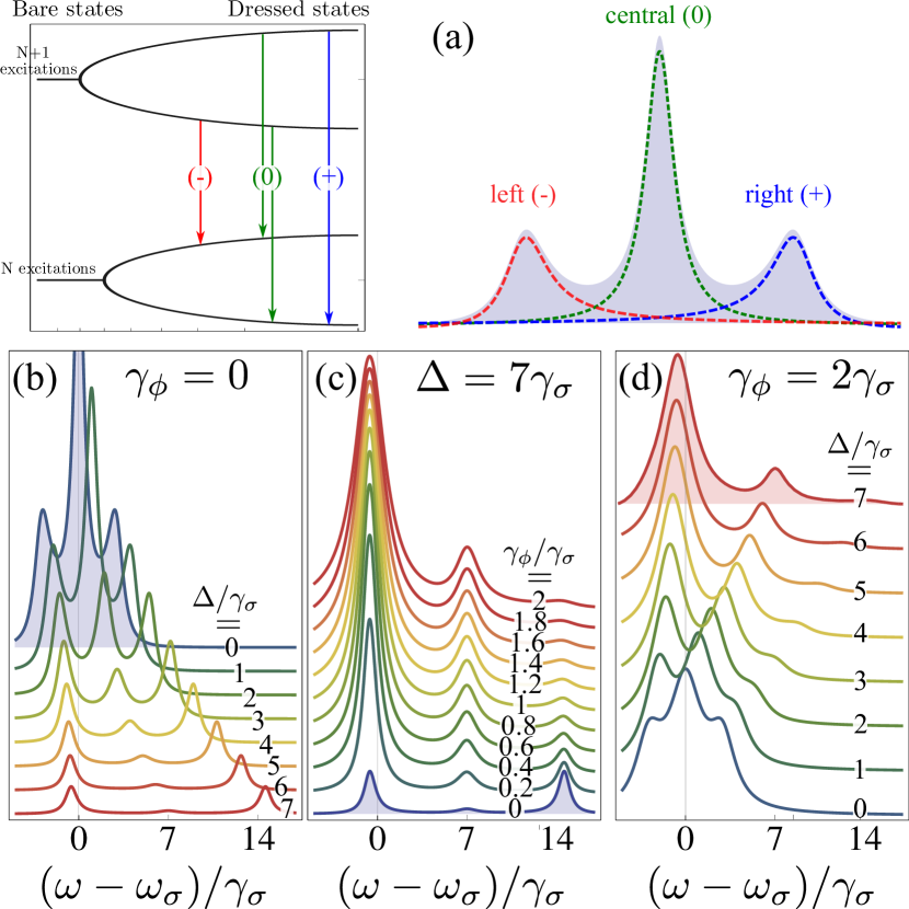
Figure 1: (Color online) (a) Origin of the peaks in the Mollow triplet: the three different frequencies ($p=0,\pm$) are found in the four possible transitions between two Jaynes-Cummings rungs at high intensities. Below, different Mollow triplets when varying detuning (b, d) or dephasing (c), with $\Omega_{\mathrm{L}}=1.5\gamma_{\sigma}$. The symmetry of the triplet is broken only under the combined action of detuning and dephasing.

The normalized spectra of emission reads in the steady state (that we set as $t=0$):

$$S_{\sigma}(\omega)=\frac{1}{\pi n_{\sigma}}\Re\int_{0}^{\infty}\langle{\sigma^{\dagger}}(0)\sigma(\tau)\rangle e^{i\omega\tau}d\tau\,.$$ (6)

Any two-time correlators can always be decomposed as a sum of complex damped exponentials del Valle (2009):

$$\langle{\sigma^{\dagger}}(0)\sigma(\tau)\rangle=n_{\sigma}\sum_{p}(L_{p}+iK_{p})e^{-i\omega_{p}\tau}e^{-\frac{\gamma_{p}}{2}\tau}\,,$$ (7)

where all the parameters, weights $L_{p}$, $K_{p}$, frequencies $\omega_{p}$ and effective decay rates $\gamma_{p}$, are real. They can be obtained by means of the quantum regression formula (see Appendix A). Eq. (6) leads to the spectrum,

$$S_{\sigma}(\omega)=\frac{1}{\pi}\sum_{p}\frac{L_{p}\frac{\gamma_{p}}{2}-K_{p}(\omega-\omega_{p})}{\big{(}\frac{\gamma_{p}}{2}\big{)}^{2}+(\omega-\omega_{p})^{2}}\,.$$ (8)

In the case of Eqs. (1–3), the spectrum has four components, that we label $p=\mathrm{coh}$, $0$, $+$, $-$. The elastic scattering component ($p=\mathrm{coh}$) is a delta peak $\delta(\omega)$ at the laser frequency ($\omega_{\mathrm{coh}}=\gamma_{\mathrm{coh}}=K_{\mathrm{coh}}=0$) with weight:

$$L_{\mathrm{coh}}=\frac{|\langle{\sigma^{\dagger}}\rangle|^{2}}{n_{\sigma}}=\frac{\gamma_{\sigma}^{2}}{8(\Omega_{\mathrm{L}}^{\mathrm{eff}})^{2}+\gamma_{\sigma}(\gamma_{\sigma}+\gamma_{\phi})}\,,$$ (9)

The inelastic scattering part is a triplet with a central peak ($p=0$) and two sidebands $p=\pm$ that carry the information about the light-matter interaction. The physical origin of these two peaks is in the transitions between the dressed states of the Jaynes-Cummings Hamiltonian at high number of excitations Cohen-Tannoudji and Reynaud (1977), as shown in Fig. 1(a). The two transitions between different types of dressed states become degenerate and form the central peak $(0)$, while transitions between the same type of dressed states give rise to the side bands. The full expression of the spectrum out of resonance is too lengthy to be given here. The resonant case formula is shorter. It reads:

$$L_{0}+iK_{0}=\frac{1}{2}\,,$$ (10a)

$$\omega_{0}=0\,,\quad\gamma_{0}=\gamma_{\sigma}+\gamma_{\phi}\,,$$ (10b)

$$L_{\pm}+iK_{\pm}=$$ (10c)

$$\frac{\frac{8\Omega_{\mathrm{L}}^{2}}{\gamma_{\sigma}(\gamma_{\sigma}+\gamma_{\phi})}\big{[}1\pm\frac{5\gamma_{\sigma}-\gamma_{\phi}}{4R_{\mathrm{L}}}\big{]}-\frac{\gamma_{\sigma}-\gamma_{\phi}}{\gamma_{\sigma}+\gamma_{\phi}}\big{[}1\pm i\frac{\gamma_{\sigma}-\gamma_{\phi}}{4R_{\mathrm{L}}}\big{]}}{4\big{(}1+\frac{8\Omega_{\mathrm{L}}^{2}}{\gamma_{\sigma}(\gamma_{\sigma}+\gamma_{\phi})}\big{)}}\,,$$

$$\omega_{\pm}=\pm\Re(R_{\mathrm{L}})\,,\quad\gamma_{\pm}=\frac{3\gamma_{\sigma}+\gamma_{\phi}}{2}\pm 2\Im(R_{\mathrm{L}})\,,$$ (10d)

where we have defined the (half) Mollow splitting:

$$R_{\mathrm{L}}=\sqrt{(2\Omega_{\mathrm{L}})^{2}-\big{(}\frac{\gamma_{\sigma}-\gamma_{\phi}}{4}\big{)}^{2}}\,.$$ (11)

Strong coupling, where the character of the dynamics of the two-time correlator is oscillating rather than damped, is defined by the appearance of this splitting ($\Re(R_{\mathrm{L}})\neq 0$), that is:

$$2\Omega_{\mathrm{L}}>|\gamma_{\sigma}-\gamma_{\phi}|/4\,.$$ (12)

We see from Eqs. (10b) and (10d) that, beyond the expected broadening of the lines, dephasing also shifts the two satellite peaks. In general, this shift brings the side peaks closer to each other, inducing the transition into weak coupling when $\gamma_{\phi}>\gamma_{\sigma}+8\Omega_{\mathrm{L}}$. However, surprisingly, the maximum splitting, for a fixed $\gamma_{\sigma}$ and $\Omega_{\mathrm{L}}$, corresponds to a nonzero dephasing, $\gamma_{\phi}=\gamma_{\sigma}$. In fact, the splitting remains different from zero, in the presence of dephasing, as long as $\gamma_{\sigma}-8\Omega_{\mathrm{L}}<\gamma_{\phi}<\gamma_{\sigma}+8\Omega_{\mathrm{L}}$. If the driving field is too weak to bring by itself the system to strong coupling ($\Omega_{\mathrm{L}}<\gamma_{\sigma}/8$), it can be aided by increasing dephasing. However, higher dephasing also blurs the spectral features. For the regimes of excitation where dephasing induces strong-coupling ($0<\gamma_{\sigma}-8\Omega_{\mathrm{L}}<\gamma_{\phi}\leq\gamma_{\sigma}$), the observed lineshape always remains single peaked.

The final expression for the Mollow triplet spectrum at resonance in presence of dephasing reads:

$$S_{\sigma}(\omega)=L_{\mathrm{coh}}\delta(\omega)+\frac{1}{2\pi}\frac{\frac{\gamma_{\sigma}+\gamma_{\phi}}{2}}{\big{(}\frac{\gamma_{\sigma}+\gamma_{\phi}}{2}\big{)}^{2}+\omega^{2}}+\\ \frac{1}{\pi}\Bigg{(}\gamma_{\sigma}\Omega_{\mathrm{L}}^{2}-\frac{\gamma_{\sigma}-\gamma_{\phi}}{16}(\gamma_{\sigma}^{2}+\omega^{2})\Bigg{)}\Bigg{/}\\ \Bigg{(}\frac{\gamma_{\sigma}^{2}+\omega^{2}}{16}\big{[}(\gamma_{\sigma}+\gamma_{\phi})^{2}+4\omega^{2}\big{]}\\ +\big{[}\gamma_{\sigma}(\gamma_{\sigma}+\gamma_{\phi})-2\omega^{2}\big{]}\Omega_{\mathrm{L}}^{2}+4\Omega_{\mathrm{L}}^{4}\Bigg{)}\,.$$ (13)

The $\delta$ scattering peak and the central peak in the first line are neatly set apart from the two side bands in the rest of the expression. This decomposition is shown in Fig. 1(a).

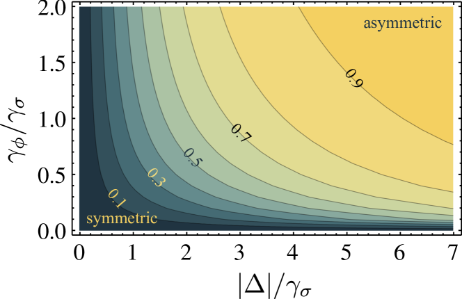
Figure 2: (Color online) Degree of asymmetry $\mathcal{V}$ of the Mollow triplet under coherent excitation, as a function of detuning $\Delta$ and pure dephasing $\gamma_{\phi}$ for $\Omega_{\mathrm{L}}=1.5\gamma_{\sigma}$. It is 0 (dark blue) when the side peaks have the same intensity and 1 (bright yellow) when one of them disappears completely.

The effect on the Mollow triplet of detuning the laser from the emitter is shown in Fig. 1(b). It spreads the side bands apart, with asymptotes $\omega_{\sigma}$ and $\omega_{\sigma}+2\Delta$, while the central peak, pinned at the driving laser frequency $\omega_{\mathrm{L}}$, gets suppressed. The scattering peak, not shown, ultimately dominates the spectrum over its incoherent part which fades away. In any case, the lineshape remains always symmetric with respect to the laser frequency (central peak), a characteristic proper to coherent excitation as we shall see later.

Out of resonance, pure dephasing has a strong qualitative effect: it breaks the above symmetry, bringing the spectrum towards the uncoupled case with only one Lorentzian peak at $\omega_{\sigma}$ with FWHM $\gamma_{\sigma}+\gamma_{\phi}$. Even a small dephasing enhances considerably the emitter peak relatively to the others, as shown in Fig. 1(c). This asymmetry becomes larger the weaker the effective laser drive, that is, for lower $\Omega_{\mathrm{L}}$ and larger $\Delta$ and dephasing. One can quantify the visibility of this asymmetry as the difference between the intensities of the two side peaks:

$$\mathcal{V}=\frac{|L_{+}-L_{-}|}{|L_{+}|+|L_{-}|}\,.$$ (14)

This is plotted in Fig. 2, where lighter (yellow) colors refer to smaller degrees of symmetry (minimum when only one peak of the two side bands survives). As a practical application, one can measure the magnitude of pure dephasing as a function of detuning from the degree of asymmetry.

III One-atom laser

In the cavity QED version of this physics, the system is described by the Jaynes-Cummings Hamiltonian Shore and Knight (1993):

$$H=\omega_{a}{a^{\dagger}}a+\omega_{\sigma}{\sigma^{\dagger}}\sigma+g({a^{\dagger}}\sigma+a{\sigma^{\dagger}})\,,$$ (15)

where also the light field is quantized, through the annihilation operator $a$. The detuning is now $\Delta=\omega_{a}-\omega_{\sigma}$ and we consider $\omega_{a}=0$ as the reference energy. The Liouvillian, $\partial_{t}\rho=\mathcal{L}\rho$, to describe this system in a dissipative context with decay ($\gamma_{c}$), incoherent pumping ($P_{c}$) and pure dephasing ($\gamma_{\phi}$) has the form del Valle et al. (2009):

$$\mathcal{L}O=i[O,H] +\sum_{c=a,\sigma}\frac{\gamma_{c}}{2}(2cO{c^{\dagger}}-{c^{\dagger}}cO-O{c^{\dagger}}c)$$ (16a)

$$+\sum_{c=a,\sigma}\frac{P_{c}}{2}(2{c^{\dagger}}Oc-c{c^{\dagger}}O-Oc{c^{\dagger}})$$ (16b)

$$+\frac{\gamma_{\phi}}{2}(2{\sigma^{\dagger}}\sigma O{\sigma^{\dagger}}\sigma-{\sigma^{\dagger}}\sigma O-O{\sigma^{\dagger}}\sigma)\,,$$ (16c)

where $\rho$ is the density matrix for the combined emitter/cavity system. The effective broadenings of the uncoupled modes are defined by $\Gamma_{a}=\gamma_{a}-P_{a}$ and $\Gamma_{\sigma}=\gamma_{\sigma}+P_{\sigma}$.

III.1 One-time correlators: populations and statistics

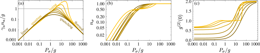
Figure 3: (Color online) Exact results computed numerically for (a) $\gamma_{a}n_{a}/g$, (b) $n_{\sigma}$ and (c) $g^{(2)}$, as a function of pumping for various systems, with $\gamma_{a}/g\in\{0.1,0.22,0.46,1,2.15,4.64,10\}$ from lighter to darker shades (top to bottom in (a)). Other parameters are $\gamma_{\sigma}=0.00334g$, from Ref. Laucht et al. (2009), and $P_{a}=\gamma_{\phi}=\Delta=0$. The different regimes of operation are designated in (a).

The light field that was previously a classical laser field was fully characterised by its intensity ($|\Omega_{\mathrm{L}}|^{2}$) and its frequency ($\omega_{\mathrm{L}}$). In the fully quantized description, correlations between the fields should be taken into account, namely, in the steady state:

$$N_{a}[n]=\langle{a^{\dagger}}^{n}a^{n}\rangle\,,\quad N_{\sigma}[n]=\langle{a^{\dagger}}^{n-1}a^{n-1}{\sigma^{\dagger}}\sigma\rangle\,,$$ (17a)

$$\tilde{N}_{a\sigma}[n]=\langle{a^{\dagger}}^{n}a^{n-1}\sigma\rangle=N^{r}_{a\sigma}[n]+iN^{i}_{a\sigma}[n]\,,$$ (17b)

with $N_{a}[n]$ and $N_{\sigma}[n]$ real and $i\tilde{N}_{a\sigma}[n]$ complex in general but real at resonance, all others being zero. The main observables that characterize the system are:

$$n_{a}=N_{a}[1]\,,\quad n_{\sigma}=N_{\sigma}[1]\quad\text{and}\quad g^{(2)}=N_{a}[2]/n_{a}^{2}\,.$$ (18)

In the following, we provide exact implicit expressions for the correlators (17), that allow an efficient numerical solution, and derive approximate analytical expressions for different regimes of excitation.

In the case without any direct cavity pumping, $P_{a}=0$, the field correlators admit a simple expression in terms of $N_{a}[n]$ (the general equations are given in Appendix B):

$$N_{\sigma}[n]= \frac{P_{\sigma}N_{a}[n-1]-\gamma_{a}N_{a}[n]}{\Gamma_{\sigma}+\gamma_{a}(n-1)}\,,$$ (19a)

$$N^{i}_{a\sigma}[n]= \frac{\gamma_{a}}{2g}N_{a}[n]\,,$$ (19b)

$$N^{r}_{a\sigma}[n]= \frac{-\Delta\gamma_{a}N_{a}[n]/g}{\Gamma_{\sigma}+\gamma_{\phi}+\gamma_{a}(2n-1)}\,.$$ (19c)

This allows to obtain a single equation for $N_{a}[n]$:

$$0=-\Big{[}\frac{1}{C_{\mathrm{eff}}[n]}+\frac{n\gamma_{a}}{\Gamma_{\sigma}+(n-1)\gamma_{a}}-\frac{2P_{\sigma}}{\Gamma_{\sigma}+n\gamma_{a}}+1\Big{]}N_{a}[n]\\ +\frac{nP_{\sigma}}{\Gamma_{\sigma}+(n-1)\gamma_{a}}N_{a}[n-1]-\frac{2\gamma_{a}}{\Gamma_{\sigma}+n\gamma_{a}}N_{a}[n+1]\,.$$ (20)

where we have introduced, respectively, the effective cooperativity, effective coupling and total decoherence (in the presence of detuning and pure dephasing):

$$C_{\mathrm{eff}}[n]= \frac{4(g_{\mathrm{eff}}[n])^{2}}{\gamma_{a}\Gamma_{\mathrm{T}}[n]}\,,$$ (21a)

$$g_{\mathrm{eff}}[n]= \frac{g}{\sqrt{1+(2\Delta/\Gamma_{\mathrm{T}}[n])^{2}}}\,,$$ (21b)

$$\Gamma_{\mathrm{T}}[n]= \Gamma_{\sigma}+\gamma_{\phi}+(2n-1)\gamma_{a}\,.$$ (21c)

Let us note that $g_{\mathrm{eff}}[n]=g$ for all $n$ at resonance or when decoherence is large as compared to the detuning. As in the case of laser excitation, the effect of detuning is to effectively diminish the coherent coupling, which magnitude is linked to the spectral overlap between modes (represented by $\Gamma_{\mathrm{T}}$). Here too, the decoupling caused by detuning can be compensated by increasing decoherence (decay or pure dephasing) since in this case the spectral overlap between the cavity and the emitter increases, bringing them effectively back to resonance. Detuning and pure dephasing only appear in the cooperativity parameter $C_{\mathrm{eff}}[n]$, as noted also by Auffèves et al. Auffèves et al. (2010). This situation is similar to the case of two coupled harmonic modes Laussy et al. (2009).

We reduced the whole steady-state problem of the Jaynes–Cummings with emitter pumping and decay to a single equation, Eq. (20), which is however a nonlinear recurrence equation with non-constant coefficients, for which there is no general method leading to an exact solution. The problem put in this form is nevertheless quite tractable numerically and we shall in the following present various limiting cases which will spell out the physics of this problem.

Since $N_{a}[0]=1$ by definition, Eq. (20) can be easily iterated numerically to provide $N_{a}[n]$ for all $n$ as a function only of the mean number of photons in the cavity, $n_{a}$. The small $n$ equations are the most important since they capture the dominant few-photons correlations. The exact expressions for $n_{\sigma}$ and $g^{2}$ in terms of $n_{a}$ are, in any case, simple enough:

$$n_{\sigma}= \frac{P_{\sigma}-\gamma_{a}n_{a}}{\Gamma_{\sigma}}\,,$$ (22a)

$$g^{(2)}= \frac{\Gamma_{\sigma}+\gamma_{a}}{2\gamma_{a}n_{a}}$$ (22b)

$$\times\Big{(}\frac{P_{\sigma}}{n_{a}\Gamma_{\sigma}}+\frac{2P_{\sigma}}{\Gamma_{\sigma}+\gamma_{a}}-\frac{\Gamma_{\sigma}+\gamma_{\phi}+\gamma_{a}}{\kappa_{\sigma}}-\frac{\gamma_{a}+\Gamma_{\sigma}}{\Gamma_{\sigma}}\Big{)}\,.$$

They are given in terms of a key parameter of the system, the Purcell rate of transfer of population from emitter to the cavity mode:

$$\kappa_{\sigma}=\frac{4(g_{\mathrm{eff}}[1])^{2}}{\gamma_{a}}\,.$$ (23)

This parameter is large for good cavities, when cavity QED is realized at its fullest: $\kappa_{\sigma}\gg g$.

One can obtain $n_{a}$ self-consistently by truncating $N_{a}[n]$ at a sufficiently high number of photons, $n_{\mathrm{max}}$, and solving numerically the resulting finite set of equations. This gives the results plotted in Fig. 3, for (a) $\gamma_{a}n_{a}/g$, (b) $n_{\sigma}$ and (c) $g^{(2)}$. In the best systems ($\gamma_{a},\gamma_{\sigma}\ll g$), we distinguish five regions in these plots, which we shall investigate in more details in the remaining of this text:

1. Linear quantum regime (or simply “linear”), where $P_{\sigma}\ll\gamma_{\sigma}$, keeping the emitter essentially in its ground state, very rarely excited.

2. Nonlinear quantum regime (or simply “quantum”), where $P_{\sigma}\sim\gamma_{\sigma}$ is enough to probe higher ($n>1$) rungs of the Jaynes-Cummings ladder, without climbing it too highly so that few photons effects remain the dominant ones.

3. Lasing or nonlinear classical regime, when $P_{\sigma}\gg\gamma_{\sigma}$ and the emitter population $\approx 0.5$, the cavity can accumulate a great number of photons and the field becomes Poissonian.

4. Self-quenching regime, when $P_{\sigma}\gtrapprox\kappa_{\sigma}/2$ starts to drive the emitter to saturation, $n_{\sigma}>1/2$, reducing the number of photons.

5. Thermal regime or linear classical regime, when $P_{\sigma}>\kappa_{\sigma}$, the emitter is always in its excited state, $n_{\sigma}\rightarrow 1$, and the dephasing induced by the pump disrupts the coherent coupling, so that the number of photons is very low again and the field becomes thermal.

Similar classifications have been proposed, for instance by Poddubny et al. Poddubny et al. (2010). In the following, we address several types of approximations, that perform to varying degrees of accuracy depending on the level of complexity involved and the regime under consideration. Some of our approximations recover known results Mu and Savage (1992); Benson and Yamamoto (1999); Poddubny et al. (2010); del Valle and Laussy (2010); Gartner (2011), however, this comparative analysis will give us, beyond good approximated formulas, valuable insights into the underlying physics. It will also allow us to determine the pumping ranges that determine each regime. As the expression for $n_{\sigma}$ and $g^{(2)}$ follow straightforwardly from that of $n_{a}$, we will not provide their explicit form in most of the cases analysed below.

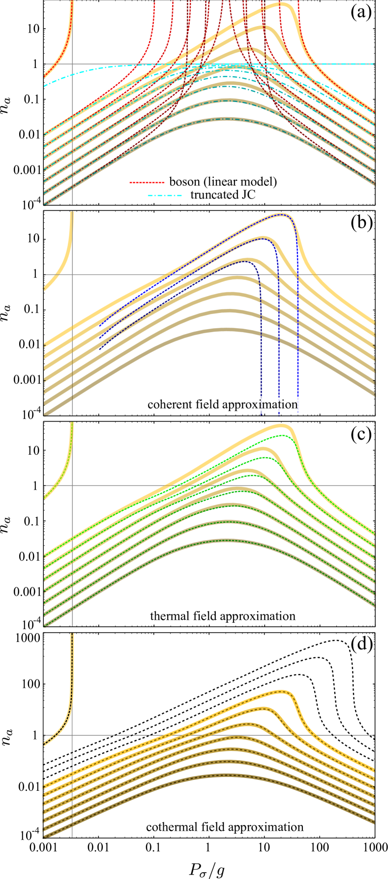
Figure 4: (Color online) Comparison between the numerical results for $n_{a}$ (from Fig. 3(a)), in thick yellowish lines, with different approximated solutions. In each panel, $\gamma_{a}$ decreases exponentially from bottom to top curves, ranking from $10g$ (darkest curve) to $0.1g$ (lightest curve). The limiting case $\gamma_{a}=0$ is also shown on the left upper corner, where the divergence is a feature of the Jaynes–Cummings model. In (a), we superimpose the linear model (dotted red) and Jaynes-Cummings truncated at one excitation (dashed blue), given by Eq. (24)(a). In (b), the approximated semiclassical solution, Eq. (32), which provides an accurate description in the lasing regime given by Eq. (61). In (c), the thermal approximation, given by Eq. (39) that converges to the models in (a) at low and high pumps. In (d), the cothermal approximation, given by the numerical solution of Eqs. (44). In this case, we extend solutions to values of $\gamma_{a}/g$ till $0.01g$, out of reach numerically. A vertical guideline marks the value of $\gamma_{\sigma}=0.00334g$. Other parameters are $P_{a}=\Delta=\gamma_{\phi}=0$.

III.1.1 Linear model approximations

In the linear regime, where the emitter is excited with very low probability, it can be well approximated by another harmonic oscillator Laussy et al. (2009). This allows to find a closed-form analytical solution:

$$n_{a}\approx\frac{\kappa_{\sigma}}{\kappa_{\sigma}(\Gamma_{\sigma}+\gamma_{a})+\Gamma_{\sigma}(\Gamma_{\sigma}+\gamma_{a}+\gamma_{\phi})}P_{\sigma}\,,$$ (24a)

$$n_{\sigma}\approx\frac{\kappa_{\sigma}+\gamma_{a}+\gamma_{\sigma}+\gamma_{\phi}}{\kappa_{\sigma}(\Gamma_{\sigma}+\gamma_{a})+\Gamma_{\sigma}(\Gamma_{\sigma}+\gamma_{a}+\gamma_{\phi})}P_{\sigma}\,.$$ (24b)

Equivalent expressions for $n_{a}$ and $n_{\sigma}$ are obtained in the first order truncation of a continuous fraction expansion of these quantities, as recently shown by Gartner Gartner (2011). They are also formally identical to those obtained by truncating the Jaynes-Cummings model at the first rung of excitation Laucht et al. (2009); Auffèves et al. (2009, 2010). The only difference is in the effective broadening $\Gamma_{\sigma}$, that appears with a $-$ sign in the case of coupled bosons, $\Gamma_{\sigma}\rightarrow\gamma_{\sigma}-P_{\sigma}$ Laussy et al. (2009), and a $+$ sign in the truncated Jaynes–Cummings model, $\Gamma_{\sigma}\rightarrow\gamma_{\sigma}+P_{\sigma}$. At $P_{\sigma}\ll\gamma_{\sigma}$, the sign becomes irrelevant with $\Gamma_{\sigma}\approx\gamma_{\sigma}$ and the population grows linearly with pumping, $n_{a}\approx C_{1}P_{\sigma}$, with the slope:

$$C_{1}=\frac{\kappa_{\sigma}}{\kappa_{\sigma}(\gamma_{\sigma}+\gamma_{a})+\gamma_{\sigma}(\gamma_{\sigma}+\gamma_{a}+\gamma_{\phi})}\,.$$ (25)

This agrees with the numerical results for $P_{\sigma}\lessapprox\gamma_{\sigma}$ as shown in Fig. 4(a). In the case where $\gamma_{\sigma}=0$, we simply have $n_{a}\approx P_{\sigma}/\gamma_{a}$. Interestingly, the two models also provide the right formula in the high pumping regime where the number of photons is low again,

$$\lim_{P_{\sigma}\rightarrow\infty}n_{a}=\frac{\kappa_{\sigma}}{P_{\sigma}}\,,$$ (26)

but the emitter is completely saturated.

The bosonic populations diverge at two values of pumping (where the denominators vanish):

$$P_{\pm}=\gamma_{\sigma}+\frac{\kappa_{\sigma}+\gamma_{a}+\gamma_{\phi}}{2}\left(1\pm\sqrt{1-\frac{4\kappa_{\sigma}\gamma_{a}}{\kappa_{\sigma}+\gamma_{a}+\gamma_{\phi}}}\right)\,.$$ (27)

For good systems with small cavity decay rates, we have $P_{-}\approx\gamma_{\sigma}$ and $P_{+}\approx\kappa_{\sigma}+\gamma_{\sigma}+\gamma_{\phi}$. At $P_{-}$, the two populations diverge but remain positive, a manifestation in this model that the system enters the lasing oscillations where both populations are “inverted”. For intermediate pumpings, where the system is in the lasing regime $P_{-}<P_{\sigma}<P_{+}$, both populations are negative, meaning that the physics in this regime is out of reach of this model. For large enough pumping, $P_{\sigma}>P_{+}$, the system exits the lasing regime as $n_{a}$ in the bosonic model converges again to the exact numerical result following Eq. (26). However, $n_{\sigma}$ remains negative for all $P_{\sigma}>P_{-}$, meaning that its population remains thereafter inverted. The bosonic model thus provides an accurate description of the transition in and out of lasing though the appearance of divergences and negative populations, as we will confirm later when linking it to the full Jaynes–Cummings system. The truncated Jaynes-Cummings formulas remain always positive and instead of a divergence, the two-level system becomes inverted, with $n_{\sigma}\rightarrow 1$ from below. Given that the number of photons is always below one, this model is not suited to describe the transitions in and out the lasing regime.

The bosonic and fermionic models provide opposite statistics for the cavity field. Two coupled harmonic oscillators under incoherent excitation are always thermal with a photon distribution $T(n)=n_{a}^{n}/(n_{a}+1)^{n+1}$ and $g^{(2)}=2$. On the other hand, truncating the Jaynes-Cummings model at one excitation means that one excludes the possibility to have two photons at a time in the cavity, which results in perfect photon antibunching, $g^{(2)}=0$. Both models provide the exact $n_{a}$ solution of the Jaynes–Cummings model in two and opposite limiting cases, namely, $\gamma_{a}\rightarrow 0$ for the bosonic model, where

$$n_{a}=\frac{P_{\sigma}}{\gamma_{\sigma}-P_{\sigma}}\,,$$ (28)

with $g^{(2)}=2$, and $\gamma_{a}\rightarrow\infty$ for the truncated Jaynes–Cummings model, where

$$n_{a}=\frac{P_{\sigma}}{\gamma_{\sigma}+P_{\sigma}}\frac{\kappa_{\sigma}}{\gamma_{a}}\,,$$ (29)

with $g^{(2)}=0$. This is seen in Fig. 4(a), where $\gamma_{a}/g=10$ (lowest curve) is already a good approximation for $\infty$, while $\gamma_{a}/g=0$ (uppermost curve) is exact. In the first limiting case, recovered by the bosonic model, the system accumulates photons in the most effective way possible, which leads to a divergence in the number of photons, also in the exact Jaynes-Cummings model. The Rabi delivery of photons is so efficient in the one-atom laser that, unless there is a leakage of photons from another channel, the accumulation of photons is unbounded. It is unlimited by the strong-coupling feed.

In the opposite limit of weak and inefficient coupling, the emitter undergoes population inversion unaffected by the cavity while the cavity gets an effective pumping of photons from $n_{\sigma}$ through a very weak Purcell rate $\kappa_{\sigma}$ Auffèves et al. (2010); Gartner (2011). For $\gamma_{a}>4g$ the truncated Jaynes-Cummings model provides a quantitatively good agreement for the entire range of pumping, as shown in Fig. 4(a), if one excludes the behaviour of $g^{(2)}$. This limit is also accounted for exactly by a series expansion in $P_{\sigma}$, given in Appendix C, since the coupling is perturbative. In this case, the system goes directly from the quantum linear to the classical linear regime.

One can obtain an exact expression for $g^{(2)}$ in the linear regime solving Eqs. (20) truncated, not at one, but at two photons, that is, for $n=1,2$ (assuming $N_{a}[3]=0$). Note that at $P_{\sigma}=0$, $N_{a}[n]=0$ for all $n$, but we are interested in the limit:

$$g_{P_{\sigma}\rightarrow 0}^{(2)}=\lim_{P_{\sigma}\rightarrow 0}\frac{N_{a}[2]}{n_{a}^{2}}\,,$$ (30)

that remains different from zero, since $N_{a}[n]\propto P_{\sigma}^{n}$. This method leads, to first order in $P_{\sigma}$, to the populations of Eq. (24) and to:

$$g_{P_{\sigma}\rightarrow 0}^{(2)}=2\frac{\kappa_{\sigma}(\gamma_{a}+\gamma_{\sigma})+\gamma_{\sigma}(\gamma_{a}+\gamma_{\sigma}+\gamma_{\phi})}{\kappa_{\sigma}(3\gamma_{a}+\gamma_{\sigma})+(\gamma_{a}+\gamma_{\sigma})(3\gamma_{a}+\gamma_{\sigma}+\gamma_{\phi})}\,.$$ (31)

This result is exact and valid for any set of parameters, as one can check by simply solving the equations to the next order of truncation ($n=1,2,3$ and $N_{a}[4]=0$). In general, $g^{(2)}\in[0,2]$ in the linear regime of the Jaynes–Cummings dynamics, although in Fig. 3(c) we only show $0\leq g^{(2)}\leq\frac{2}{3}$ since we have chosen $\gamma_{\sigma}\approx 0$.

III.1.2 Semiclassical approximation

Given that, as shown in Fig. 3(c), the cavity field becomes Poissonian in the lasing regime, we can find good approximated solutions for the steady state under the assumption $\mathrm{T}[n]=e^{-n_{a}}n_{a}^{n}/n!$, which leads to $N_{a}[n]=n_{a}^{n}$. To establish the lasing in strong-coupling regime, one also needs a good cavity, so we shall assume $\gamma_{a}\ll g$, and high enough pumping, $P_{\sigma}\gg\gamma_{\sigma},\gamma_{a}$. Plugging $N_{a}[n]=n_{a}^{n}$ into Eq. (20) and solving the resulting equation for $n=1$, or equivalently, imposing $g^{(2)}=1$ in Eq. (22b), gives

$$n_{a}\approx\frac{\Gamma_{\sigma}}{2\gamma_{a}}\Big{(}1-\frac{2\gamma_{\sigma}}{\Gamma_{\sigma}}-\frac{\Gamma_{\sigma}+\gamma_{\phi}}{\kappa_{\sigma}}\Big{)}\,.$$ (32)

This is a very good approximation for the region where the cavity field behaves classically Mu and Savage (1992); Karlovich and Kilin (2001), equivalent to solving the $n=0$ equation in Eqs. (20) del Valle and Laussy (2010); Gartner (2011). The probability of finding the emitter in its excited state reads:

$$n_{\sigma}\approx\frac{1}{2}\Big{(}1+\frac{\Gamma_{\sigma}+\gamma_{\phi}}{\kappa_{\sigma}}\Big{)}\,.$$ (33)

The approximated $n_{a}$ is plotted with blue dashed lines in Fig. 4(b) for comparison with the numerical results and exhibits a remarkable agreement for a large pumping range of practical interest (the axis is in log scale). Similar agreement is found for $n_{\sigma}$ del Valle and Laussy (2010).

The two expressions for the populations have a straightforward interpretation. Two parameters determine the populations (neglecting for the sake of simplicity the small correction brought by the emitter decay, $2\gamma_{\sigma}/\Gamma_{\sigma}\ll 1$): the “cavity feeding” and the “emitter feeding” efficiencies, defined as $F_{a}=\Gamma_{\sigma}/(2\gamma_{a})$ and $F_{\sigma}=(\Gamma_{\sigma}+\gamma_{\phi})/\kappa_{\sigma}$, respectively. They follow as:

$$n_{a}\approx F_{a}(1-F_{\sigma})\quad\mathrm{and}\quad n_{\sigma}\approx(1+F_{\sigma})/2\,.$$ (34)

The cavity population increases linearly with pumping ($n_{a}\approx F_{a}$) while the emitter is half occupied ($n_{\sigma}\approx 1/2$). This is the range of pumping with the most effective accumulation of photons in the cavity, as the incoherent processes are small enough not to disrupt the coherent coupling dynamics. All the excitations injected into the emitter are transferred into the cavity. We already have seen that there is a linear relationship between $n_{a}$ and $P_{\sigma}$ in the—aptly denominated—linear regime, as given by Eq. (25). A similar linear relationship $n_{a}\approx C_{2}P_{\sigma}$ also holds in the lasing regime, when $P_{\sigma}\ll\kappa_{\sigma}$ but beyond the quantum regime, $P_{\sigma}>\gamma_{a},\gamma_{\sigma}$, this time with a slope $C_{2}$ defined as:

$$C_{2}=\frac{1}{2\gamma_{a}}.$$ (35)

The transition between the two types of linear behaviours $n_{a}\approx C_{i}P_{\sigma}$, $i=1\rightarrow 2$, and the question of the threshold in this process is an interesting subject Clemens et al. (2004) that would bring us too far astray and that we postpone to another work del Valle et al. (2011). We will only comment in the present text that this intermediate region is the less liable to the types of approximation that we derive here, since it lies at the frontier between the very few and the very large number of excitations, and no good approximation can reproduce it to a high degree of accuracy other than by keeping track of all correlations between the particles, which, being a $N$ body type of problem, implies a numerical procedure. We call this intermediate region the “quantum nonlinear” or simply the “quantum” regime.

When the pumping is sizable as compared to $\kappa_{\sigma}$, the emitter occupation starts to show signs of saturation, increasing linearly with pumping, and quenching the linear increase of the cavity population. $F_{\sigma}$ represents therefore the degree to which the pumping succeeds in populating the emitter itself, against the coherent exchange of population that feeds the cavity with efficiency $F_{a}$. The maximum population of the cavity

$$\max(n_{a})\approx\frac{\kappa_{\sigma}}{8\gamma_{a}}\big{(}1-\frac{4\gamma_{\sigma}+2\gamma_{\phi}}{\kappa_{\sigma}}\big{)}\,,$$ (36)

is reached at the intermediate rate

$$P_{\sigma}|_{\max(n_{a})}\approx\frac{\kappa_{\sigma}}{2}\big{(}1-\frac{2\gamma_{\sigma}+\gamma_{\phi}}{\kappa_{\sigma}}\big{)}\,.$$ (37)

The present approximated expressions are valid until $n_{\sigma}$ approaches 1, then, the self-quenching dominates the dynamics and $n_{a}\rightarrow 0$, at around:

$$P_{\mathrm{max}}\approx\kappa_{\sigma}-3\gamma_{\sigma}-2\gamma_{\phi}\,,$$ (38)

that is, when the pump reaches the effective transfer rate of excitation towards the cavity mode. At this point the statistics changes to thermal due to pump-induced decoherence. Note that $P_{\mathrm{max}}\approx P_{+}$, found in the previous subsection when analysing the bosonic model.

III.1.3 Thermal approximation

Assuming a thermal state for the cavity field, with statistics $T(n)=n_{a}^{n}/(n_{a}+1)^{n+1}$ and thus with $N_{a}[n]=n!n_{a}^{n}$, satisfies in good approximation Eqs. (20) when the system undergoes self-quenching and gets driven into the thermal regime ($P_{\sigma}>\kappa_{\sigma}$). The $n_{a}$ obtained from the equation ($n=1$), or equivalently, imposing $g^{(2)}=2$ in Eq. (22b), reads:

$$n_{a}\approx\frac{1}{8\gamma_{a}}\Big{\{}(\Gamma_{\sigma}+\gamma_{a})\times\\ \sqrt{\frac{16P_{\sigma}\gamma_{a}/\Gamma_{\sigma}}{\Gamma_{\sigma}+\gamma_{a}}+\big{[}1+\frac{\Gamma_{\sigma}+\gamma_{a}+\gamma_{\phi}}{\kappa_{\sigma}}-\frac{2P_{\sigma}}{\Gamma_{\sigma}+\gamma_{a}}+\frac{\gamma_{a}}{\Gamma_{\sigma}}\big{]}^{2}}\\ -\Gamma_{\sigma}\big{(}\frac{\Gamma_{\sigma}+\gamma_{\phi}}{\kappa_{\sigma}}+\frac{2\gamma_{\sigma}}{\Gamma_{\sigma}}-1\big{)}-\gamma_{a}\big{(}\frac{2\Gamma_{\sigma}+\gamma_{\phi}}{\kappa_{\sigma}}+2\big{)}\\ -\frac{\gamma_{a}^{2}}{\Gamma_{\sigma}}\big{(}\frac{\Gamma_{\sigma}}{\kappa_{\sigma}}+1\big{)}\Big{\}}\,.$$ (39)

This solution converges to the linear result of Eq. (24) to first order in $P_{\sigma}$ when $P_{\sigma}<\gamma_{\sigma}$. The opposite limit, well into the thermal region, is that already found with Eq. (26) to first order in $1/P_{\sigma}$, which provides the decreasing tail at large pumpings, as shown in Fig. 4. The lines converge to the same universal curve when plotting $\gamma_{a}n_{a}/g$ in Fig. 3(a). In the intermediate region, it provides a good approximation when the system is not good enough to lase, at large dissipation rates, similarly to the truncated Jaynes-Cummings formula. Of course, having $g^{(2)}=2$ throughout, does not, in general, represent well the statistics.

Fig. 4(c) may seem to shown that Eq. (39) captures the qualitative behaviour of $n_{a}$ even in the lasing regime. It does not, however, provide the change into the linear lasing slope from $n_{a}\sim C_{1}P_{\sigma}$ to $C_{2}P_{\sigma}$, discussed in the previous subsection, which is a serious conceptual shortcoming.

In two particular cases, the thermal solution becomes exact for Eq. (20), namely, $\gamma_{c}=P_{c}=0$ with $c=a$ (previously discussed) on the one hand and its counterpart $c=\sigma$ on the other hand. In both cases $N_{a\sigma}=0$ and $N_{\sigma}[n]=\bar{n}_{\sigma}N_{a}[n-1]$ with $N_{a}[n]=n!\bar{n}_{a}^{n}$, where:

$$\bar{n}_{a}=\frac{P_{c}}{\gamma_{c}-P_{c}}\quad\text{and}\quad\bar{n}_{\sigma}=\frac{P_{c}}{\gamma_{c}+P_{c}}\,.$$ (40)

The steady state in this case is two uncorrelated thermal fields at the same temperature. This is independent of the coupling strength $g$, which only determines the speed at which this steady state is achieved. Although the discontinuity at $g=0$ might seem counterintuitive, it is physically clear that the thermal equilibrium does not otherwise depend on details of the microscopic couplings. The case $P_{\sigma}=\gamma_{\sigma}=0$, that corresponds to thermal excitation of the cavity mode only, presents interesting aspects which we also postpone to a future work.

The case $P_{a}=0=\gamma_{a}=0$, appearing in Fig. 4(c) as the uppermost exact curve, diverges, as we noted previously, at $P_{\sigma}\geq\gamma_{\sigma}$, meaning that the system does not have a steady state but rather its intensity grows without bounds. This is to be interpreted as the instability accompanying the transition into lasing Karlovich and Kilin (2001).

III.1.4 Cothermal approximation

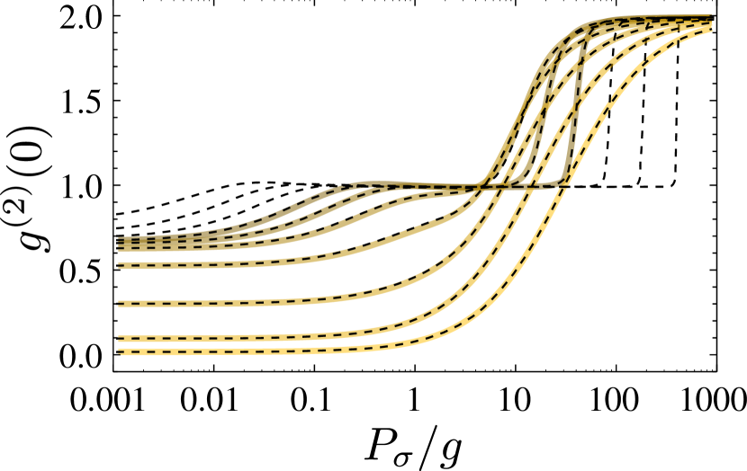
Figure 5: (Color online) Comparison between the numerical $g^{(2)}$ (in thick lines) and the cothermal approximation (dashed lines), from Eq. (43) with $n_{a}$ of Fig. 4. It interpolates neatly between the lasing and the thermal regions ($1\rightarrow 2$) but also provides a very good agreement in the linear regime.

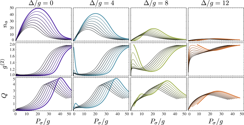
Figure 6: (Color online) (a) $n_{a}$, (b) $g^{(2)}$ and (c) $Q$-Mandel parameter, as a function of the pumping rate, extracted with the cothermal approximation. Detuning is fixed in each column to the value while pure dephasing increases from $0$ (thick curves) to $12g$ (dashed curves) in steps of $2g$. Detuning brings a threshold for lasing and while dephasing can help to reduce it, it also makes the system less robust to quenching. Parameters are $\gamma_{a}=0.1g$, $P_{a}=0=\gamma_{\sigma}=0$.

A very good quantitative approximation for the whole pumping range is obtained assuming that the field is in a so-called cothermal state Laussy et al. (2006), which is the field with, in average, $n_{a}^{\mathrm{coh}}$ coherent photons and $n_{a}^{th}$ thermal photons (with a total cavity population $n_{a}=n_{a}^{th}+n_{a}^{\mathrm{coh}}$). In this case, the photonic statistics reads:

$$\mathrm{T}[n]=e^{-n_{a}^{\mathrm{coh}}/(1+n_{a}^{th})}\frac{(n_{a}^{th})^{n}}{(1+n_{a}^{th})^{n+1}}\mathrm{L}_{n}[\frac{-n_{a}^{\mathrm{coh}}}{n_{a}^{th}(1+n_{a}^{th})}]\,,$$ (41)

and moments of the distribution are:

$$N_{a}[n]=n!(n_{a}^{th})^{n}\mathrm{L}_{n}[-\frac{n_{a}^{\mathrm{coh}}}{n_{a}^{th}}]\,,$$ (42)

with $\mathrm{L}_{n}$ the $n$-th Laguerre polynomial. The second order coherence function is

$$g^{(2)}=2-\big{(}\frac{n_{a}^{\mathrm{coh}}}{n_{a}}\big{)}^{2}\,.$$ (43)

One can write the set of Eqs. (20) for $n=$1, 2 using the parametrization of Eq. (42):

$$0=\Big{[}\frac{1}{C_{\mathrm{eff}}[1]}+\frac{\gamma_{a}}{\Gamma_{\sigma}}-\frac{2P_{\sigma}}{\Gamma_{\sigma}+\gamma_{a}}+1\Big{]}n_{a}$$

$$-\frac{P_{\sigma}}{\Gamma_{\sigma}}+\frac{2\gamma_{a}}{\Gamma_{\sigma}+\gamma_{a}}[2n_{a}^{2}-(n_{a}^{\mathrm{coh}})^{2}]\,,$$ (44a)

$$0=\Big{[}\frac{1}{C_{\mathrm{eff}}[2]}+\frac{2\gamma_{a}}{\Gamma_{\sigma}+2\gamma_{a}}-\frac{2P_{\sigma}}{\Gamma_{\sigma}+2\gamma_{a}}+1\Big{]}[2n_{a}^{2}-(n_{a}^{\mathrm{coh}})^{2}]$$

$$-\frac{2P_{\sigma}}{\Gamma_{\sigma}+\gamma_{a}}n_{a}+\frac{2\gamma_{a}}{\Gamma_{\sigma}+2\gamma_{a}}[6n_{a}^{3}-9n_{a}(n_{a}^{\mathrm{coh}})^{2}+4(n_{a}^{\mathrm{coh}})^{3}]\,.$$ (44b)

Equations (44) can be easily solved numerically (two coupled nonlinear equations), extracting the physical solution $n_{a}$, $n_{a}^{\mathrm{coh}}\geq 0$. They yield an excellent agreement with the complete numerical solution as shown in Fig. 4(d) for the cavity population and Fig. 5 for $g^{(2)}$. We took advantage of this to extend the results to cases out of reach of our numerical procedure, namely, $\gamma_{a}/g$ down to $0.01$, shown on Figs. 4 and 5 as the dashed lines only, without the corresponding numerical calculation. The transitions from the linear regime to lasing and from lasing to the thermal regime are well accounted for within this approximation. Although they are not exact, they provide a fairly good quantitative description of the entire pumping range for any set of parameters, particularly of the quantum regime which eludes most approximation schemes.

The transition into a thermal field can be induced by increasing the incoherent pumping but also other sources of decoherence such as dissipation, pure dephasing or detuning. In Fig. 6, we plot the extracted $n_{a}$ and $g^{(2)}$, respectively, under the cothermal approximation, as a function of pumping, when increasing detuning and pure dephasing. The lasing to thermal transition is even more apparent in the Mandel-$Q$ parameter, defined as $Q=n_{a}(g^{(2)}-1)$, featuring it with a broad peak, as shown in the third row of Fig. 6. Both detuning and dephasing are clearly detrimental for the intensity and coherence in the self-quenching regime but they may compensate each other in the transition from the linear regime into lasing. Fig. 6 shows the appearance of a threshold in the presence of detuning (at small pumping the thermal fraction increases), due to the reduction of $g_{\mathrm{eff}}$ P. R. Rice (1994). Adding dephasing, $\gamma_{\phi}$, may compensate this reduction and smoothen the threshold up to a certain point (as it also increases to the total decoherence rate $\Gamma_{\mathrm{T}}$). This observation was made by Auffèves et al. Auffèves et al. (2010). In general, the maximum intensity, max($n_{a}$), and coherence achieved, always decrease with both detuning and dephasing. However, detuning makes it occur at higher pumpings while dephasing does at lower ones. Pure dephasing is thus indeed making both transitions, from quantum to lasing and from lasing to self-quenching, occur at smaller pumping.

III.2 Density matrix

We have obtained in the previous section good approximations for the statistics of the cavity field, $\mathrm{T}[n]$, as well as the main quantities of interest such as $n_{a}$. To compute the photoluminescence spectrum, what we will do in next section, we also need the full density matrix in the steady state. In the very strong-coupling regime, we can relate it analytically to $\mathrm{T}[n]$, as we show in this section.

The full statistics is most conveniently obtained from the master equation with elements $\rho_{m,i;n,j}$ for $m$, $n$ photons and $i$, $j$ excitation of the emitter ($m,n\in\mathbf{N}$, $i,j\in\{0,1\}$). Rather than to consider the equations of motion for the matrix elements directly, it is clearer and more efficient to consider only elements that are nonzero in the steady state. These are:

$$\mathrm{p}_{0}[n]=\rho_{n,0;n,0}\,,\quad\mathrm{p}_{1}[n]=\rho_{n,1;n,1}\,,\quad\mathrm{q}[n]=\rho_{n,0;n-1,1}\,,$$ (45)

and correspond to, respectively, the probability to have $n$ photons with ($\mathrm{p}_{1}$) or without ($\mathrm{p}_{0}$) excitation of the emitter, and the coherence element between the states $\left|n,0\right\rangle$ and $\left|n-1,1\right\rangle$, linked by the Hamiltonian Eq. (15). Both $p_{0}$ and $p_{1}$ are real. It is convenient to separate $q$ into its real and imaginary parts, $\mathrm{q}[n]=\mathrm{q}_{\mathrm{r}}[n]+i\mathrm{q}_{\mathrm{i}}[n]$, as they play different roles in the dynamics. The equations for these quantities are derived from the Liouvillian equation (16). They read (their full form is given in Appendix B):

$$\partial_{t}\mathrm{p}_{0}[n+1]= \mathcal{D}_{\mathrm{phot}}\{\mathrm{p}_{0}[n+1]\}$$ (46a)

$$-P_{\sigma}\mathrm{p}_{0}[n+1]+\gamma_{\sigma}\mathrm{p}_{1}[n+1]$$

$$-2g\sqrt{n+1}\mathrm{q}_{\mathrm{i}}[n+1]\,,$$

$$\partial_{t}\mathrm{p}_{1}[n]= \mathcal{D}_{\mathrm{phot}}\{\mathrm{p}_{1}[n]\}$$ (46b)

$$-\gamma_{\sigma}\mathrm{p}_{1}[n]+P_{\sigma}\mathrm{p}_{0}[n]+2g\sqrt{n+1}\mathrm{q}_{\mathrm{i}}[n+1]\,,$$

$$\partial_{t}\mathrm{q}_{\mathrm{i}}[n+1]= \mathcal{D}_{\mathrm{phot}}\{\mathrm{q}_{\mathrm{i}}[n+1]\}$$

$$-\Big{[}\frac{\Gamma_{\sigma}+\gamma_{\phi}}{2}+\frac{2\Delta^{2}}{\Gamma_{\sigma}+\gamma_{\phi}}\Big{]}\mathrm{q}_{\mathrm{i}}[n+1]$$

$$+g\sqrt{n+1}(\mathrm{p}_{0}[n+1]-\mathrm{p}_{1}[n])\,,$$ (46c)

where we have separated the cavity dynamics into a superoperator $\mathcal{D}_{\mathrm{phot}}$, which exact expression is given in the Appendix. If this photonic dynamics is much slower than the rest, that is $\gamma_{a},P_{a}\ll\Gamma_{\sigma},g$, one can solve the emitter dynamics separately, ignoring $\mathcal{D}_{\mathrm{phot}}$ Scully and Zubairy (2002); Mu and Savage (1992). This assumes that the photon distribution $\mathrm{T}[n]=\mathrm{p}_{0}[n]+\mathrm{p}_{1}[n]$ does not change during the excitation and interaction with the emitter that happens at a timescale, of order $1/P_{\sigma}$ or $1/g$, much faster than the photon one, of order $1/\gamma_{a}$. This approximation becomes exact for the perfect cavity, when $\gamma_{a}=0$ (and $P_{a}=0$, which we already assumed), which is why the system admits an exact solution (cf. Eq. (40)). Neglecting the photon dynamics allows one to link all the density matrix elements with the photon statistics $\mathrm{T}[n]$:

$$\mathrm{p}_{0}[n+1]\approx$$ (47a)

$$\frac{\kappa_{a}(n+1)\Big{(}\frac{P_{\sigma}}{\Gamma_{\sigma}}\mathrm{T}[n]+\frac{\gamma_{\sigma}}{\Gamma_{\sigma}}\mathrm{T}[n+1]\Big{)}+\gamma_{\sigma}\mathrm{T}[n+1]}{2\kappa_{a}(n+1)+\Gamma_{\sigma}}\,,$$

$$\mathrm{p}_{1}[n]\approx$$ (47b)

$$\frac{\kappa_{a}(n+1)\Big{(}\frac{P_{\sigma}}{\Gamma_{\sigma}}\mathrm{T}[n]+\frac{\gamma_{\sigma}}{\Gamma_{\sigma}}\mathrm{T}[n+1]\Big{)}+P_{\sigma}\mathrm{T}[n]}{2\kappa_{a}(n+1)+\Gamma_{\sigma}}\,,$$

$$\mathrm{q}_{\mathrm{i}}[n+1]\approx\frac{\kappa_{a}\sqrt{n+1}}{2g}(\mathrm{p}_{0}[n+1]-\mathrm{p}_{1}[n])$$ (47c)

$$=-\frac{\kappa_{a}\sqrt{n+1}}{2g}\frac{P_{\sigma}\mathrm{T}[n]-\gamma_{\sigma}\mathrm{T}[n+1]}{2\kappa_{a}(n+1)+\Gamma_{\sigma}}\,.$$

where

$$\kappa_{a}=\frac{4(g_{\mathrm{eff}}[1])^{2}}{\Gamma_{\sigma}+\gamma_{\phi}}$$ (48)

is the Purcell rate of transfer of population from the cavity mode to the emitter (cf. Eq. (23)) and $g_{\mathrm{eff}}$ follows the definition in Eq. (21) for negligible $\gamma_{a}$. Note that $\mathrm{p}_{0}[n]+\mathrm{p}_{1}[n]$ is not strictly equal to $\mathrm{T}[n]$, due to our approximations, but the numerical discrepancy is small in the regime of interest where the number of photons is high and $n\approx n+1$. In particular, the equality holds exactly in the aforementioned case of $\gamma_{a}=P_{a}=0$, thanks to some nontrivial simplifications of the expressions when $\mathrm{T}[n]$ is thermal.

III.3 Two-time correlators

We now turn to the problem of the steady state optical emission spectrum, that consists in computing two-time correlators of the type $\langle{c^{\dagger}}(0)c(\tau)\rangle$ with $c=a$, $\sigma$. We can link the two time correlators to the quantities derived in the previous sections following an implementation of the quantum regression theorem that relies explicitly on the density matrix $\rho$:

$$\langle{c^{\dagger}}(0)c(\tau)\rangle=\sum_{k,l}\rho^{c}_{[k;l]}(\tau)\left\langle l\right|c\left|k\right\rangle\,,$$ (49)

where $\rho^{c}_{[k;l]}(\tau)=\langle{c^{\dagger}}(\left|l\right\rangle\left\langle k\right|)(\tau)\rangle$ is in the Schrödinger picture, where the states evolve and operators have their steady state values Mølmer (1996). The indices $k$, $l$ go through all the states in the system Hilbert space ($k=(k_{1},k_{2})$ with $k_{1}=0,1,\ldots,n_{\mathrm{max}}$ for the photons and $k_{2}=0,1$ for the emitter). The elements $\rho^{c}_{[k;l]}$ follow the same master equation as the density matrix elements $\rho_{[k;l]}$. Since similar approximations can also be naturally implemented, this will allow us to provide closed-form solutions for the two-time correlators, as is detailed in Appendix D. We give here the main lines of the derivations and introduce the key quantities that lead to the final result. We single out, again, only the nonzero elements. For two-time correlators, they can be gathered in four functions of $n$:

$$S_{i}[n]\equiv\rho^{c}_{[n,i;n-1,i]}\,,\quad i=0,1\,,\quad n\geq 0\,,$$ (50a)

$$Q[n]\equiv\rho^{c}_{[n,1;n,0]}\,,\quad n\geq 0\,,$$ (50b)

$$V[n]\equiv\rho^{c}_{[n,0;n-2,1]}\,,\quad n\geq 1\,.$$ (50c)

The two-times correlators follow from these quantities (with $c=\sigma$, $a$ respectively) as:

$$\langle{\sigma^{\dagger}}(0)\sigma(\tau)\rangle=\sum_{n=0}^{\infty}Q[n]\,,$$ (51a)

$$\langle{a^{\dagger}}(0)a(\tau)\rangle=\sum_{n=0}^{\infty}(\sqrt{n+1}S_{0}[n+1]+\sqrt{n}S_{1}[n])\,.$$ (51b)

Each term $n$ of these sums accounts for the transitions between the rungs $n+1$ and $n$, as in the case of spontaneous emission del Valle et al. (2009), the first rung, being given by $n=0$.

The equations of motion for the quantities in Eqs. (50) are extracted from the master equation (cf. Eq. 90), and can also be, like for the single time dynamics, separated into a slow photonic dynamics embedded in a superoperator $\mathcal{D}_{\mathrm{phot}}$ on the one hand, and a fast emitter and coupling dynamics on the other hand:

$$\partial_{\tau}S_{0}[n+1]= \mathcal{D}_{\mathrm{phot}}\{S_{0}[n+1]\}$$ (52a)

$$-P_{\sigma}S_{0}[n+1]+\gamma_{\sigma}S_{1}[n+1]$$

$$+ig(\sqrt{n}V[n+1]-\sqrt{n+1}Q[n])\,,$$

$$\partial_{\tau}S_{1}[n]= \mathcal{D}_{\mathrm{phot}}\{S_{1}[n]\}$$ (52b)

$$+P_{\sigma}S_{0}[n]-\gamma_{\sigma}S_{1}[n]$$

$$-ig(\sqrt{n+1}V[n+1]-\sqrt{n}Q[n])\,,$$

$$\partial_{\tau}Q[n]= \mathcal{D}_{\mathrm{phot}}\{Q[n]\}$$ (52c)

$$-\Big{(}\frac{\Gamma_{\sigma}+\gamma_{\phi}}{2}-i\Delta\Big{)}Q[n]$$

$$+ig(\sqrt{n}S_{1}[n]-\sqrt{n+1}S_{0}[n+1])\,,$$

$$\partial_{\tau}V[n+1]= \mathcal{D}_{\mathrm{phot}}\{V[n+1]\}$$ (52d)

$$-\Big{(}\frac{\Gamma_{\sigma}+\gamma_{\phi}}{2}+i\Delta\Big{)}V[n+1]$$

$$+ig(\sqrt{n}S_{0}[n+1]-\sqrt{n+1}S_{1}[n])\,,$$

for $n\geq 1$. After some long, but straightforward algebra, we can express $S_{0,1}[n]$ and $Q[n]$ in terms of $\mathrm{p}_{0,1}[n]$ and $\mathrm{q}_{i}[n]$, which, in turn, are expressed in terms of the statistics $\mathrm{T}[n]$. This can be done for arbitrary parameters, including detuning. However, simple expressions are possible only at resonance, where we can write Eq. (49) as:

$$\langle{c^{\dagger}}(0)c(\tau)\rangle =E^{c}+n_{c}\sum_{n=0}^{\infty}[$$

$$C_{\mathrm{I}}^{c}[n]e^{-iR_{\mathrm{I}}[n]\tau}e^{-(3\Gamma_{\sigma}+\gamma_{\phi})\tau/4}+\text{R.s.i.}$$

$$C_{\mathrm{O}}^{c}[n]e^{-iR_{\mathrm{O}}[n]\tau}e^{-(3\Gamma_{\sigma}+\gamma_{\phi})\tau/4}+\text{R.s.i.}]\,.$$ (53)

“R.s.i” stands for “Rabi sign inversion” and is the operation that consists in changing the sign of $R_{\mathrm{I},\mathrm{O}}$ keeping all other quantities the same. The first term $E^{c}$ that factors out of the sum, is independent of $\tau$, due to the approximation of very large photonic lifetime. It is discussed separately in section IV.3. The most fundamental quantities that arise in the above treatment are the $n$th manifold inner and outer (half) Rabi frequencies:

$$R_{\mathrm{O},\mathrm{I}}[n]=\sqrt{g^{2}(\sqrt{n+1}\pm\sqrt{n})^{2}-\Big{(}\frac{\Gamma_{\sigma}-\gamma_{\phi}}{4}\Big{)}^{2}}\,.$$ (54)

The (half) Rabi frequency of the linear regime, $R_{0}$ is recovered as the particular case $n=0$ with

$$R_{0}=R_{\mathrm{O}}[0]=R_{\mathrm{I}}[0]=\sqrt{g^{2}-\Big{(}\frac{\Gamma_{\sigma}-\gamma_{\phi}}{4}\Big{)}^{2}}\,.$$ (55)

The coefficient $C_{\mathrm{I}}^{c}[n]$ (id. for $C_{\mathrm{O}}^{c}[n]$) are complex quantities in general that we decompose into their real and imaginary part as

$$C_{\mathrm{I}}^{c}[n]=L_{\mathrm{I}}^{c}[n]+iK_{\mathrm{I}}^{c}[n]$$ (56)

They are a function of $R_{\mathrm{I}}[n]$ (and $C_{\mathrm{O}}$ of $R_{\mathrm{O}}[n]$).

As stated previously, the coefficients $C_{\mathrm{I},\mathrm{O}}^{c}[n]$ are written in terms of the system parameters and the steady state photon distribution $\mathrm{T}[n]$ only. Their general full expression are too long to be given. Only for the simplest case of $\gamma_{\sigma}$, $\gamma_{\phi}=0$ and $c=\sigma$, the expressions simplify sufficiently to be reproduced here:

$$C_{\mathrm{I},\mathrm{O}}^{\sigma}[n]=\frac{\alpha_{\mathrm{I},\mathrm{O}}^{\sigma}[n]}{n_{\sigma}}\mathrm{T}[n]+\frac{\beta_{\mathrm{I},\mathrm{O}}^{\sigma}[n]}{n_{\sigma}}\mathrm{T}[n-1]$$ (57)

where:

$$\alpha_{\mathrm{I},\mathrm{O}}^{\sigma}[n] =\frac{\left(\frac{P_{\sigma}}{2}\right)^{2}+g^{2}(1+n)}{P_{\sigma}^{2}+8g^{2}(1+n)}+\frac{iP_{\sigma}}{4R_{\mathrm{I},\mathrm{O}}[n]}\times$$ (58a)

$$\frac{\left(\frac{P_{\sigma}}{2}\right)^{2}-g^{2}(1+n\mp 2\sqrt{n(1+n)})}{P_{\sigma}^{2}+8g^{2}(1+n)}\,,$$

$$\beta_{\mathrm{I},\mathrm{O}}^{\sigma}[n] =\pm g^{2}P_{\sigma}^{2}(4+3\frac{iP_{\sigma}}{4R_{\mathrm{I},\mathrm{O}}[n]})\times$$ (58b)

$$\frac{2g^{2}(\sqrt{n(1+n)}\pm n)+P_{\sigma}^{2}(\sqrt{n(1+n)}\mp n)}{4(8g^{2}n+P_{\sigma}^{2})(4g^{4}+4g^{2}P_{\sigma}^{2}(1+2n)+P_{\sigma}^{4})}\,,$$

where the notations $\pm$ and $\mp$ associate $I$ to the upper sign and $O$ to the lower one.

IV Mollow triplet under incoherent excitation

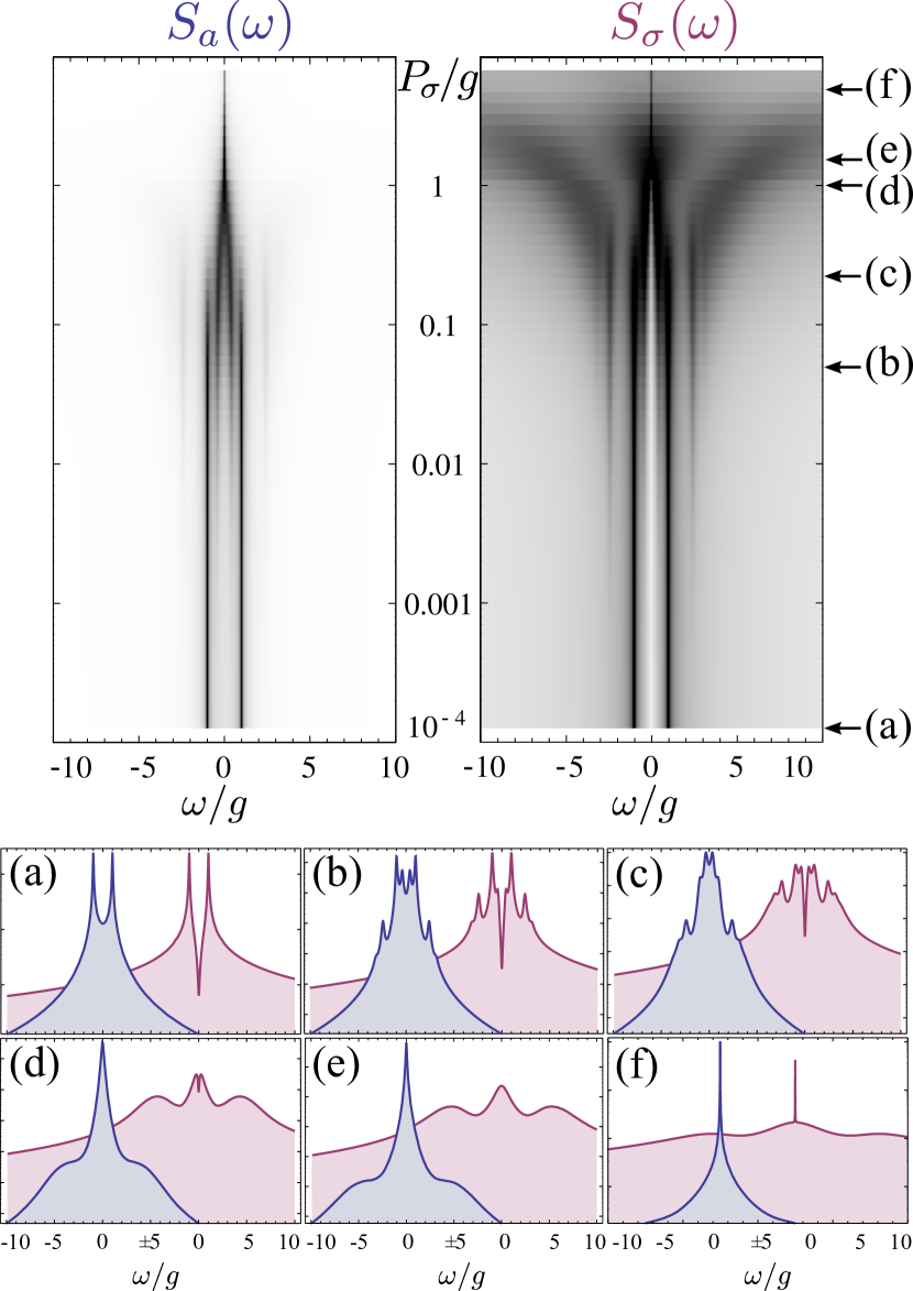
Figure 7: (Color online) Cavity (left blue) and emitter (right pink) spectra of emission computed numerically. As a function of pumping, a transition from (a) the quantum linear regime to (f) lasing can be followed passing through (b) the quantum nonlinear regime that (c) melts into (d) and (e) structures of much reduced complexity, namely, triplets. A Mollow triplet is neatly visible in the emitter spectrum, whereas the cavity gives rise to a single narrowing line. Note that in the cuts (a–f), spectra are displayed in log-scale. Parameters are $\gamma_{a}=0.1g$, $\gamma_{\sigma}=0.00334g$, $P_{a}=\gamma_{\phi}=\Delta=0$.

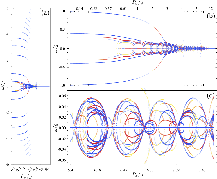
Figure 8: (Color online) Lasing as a condensation of dressed states: transitions energies between the dressed states when solving numerically the dynamics exactly are shown. The color code (online) has blue shades corresponding to a positive weight of the transition in the cavity emission and red shades corresponding to a negative weight. In (a) all regimes are shown over all energies, in (b) a close-up of (a) is given for frequencies $|\omega_{p}|<g$ lying between the vacuum Rabi splitting, in (c) a close-up of (b) is given in the lasing regime, showing an extremely complex structure of the exact solution obtained in the full-quantization picture, although the final result washes out completely most of this underlying information, to provide only the single narrow line of a lasing system.

The luminescence spectra can, like all other quantities, be obtained “exactly” through numerical computations Löffler et al. (1997); del Valle et al. (2009). In our case, computing Eqs. (52) and applying the definition of Eq. (8) for the power spectra, one arrives to results such as those shown in Fig. 7, where PL spectra are computed both for the cavity and the emitter, as a function of pumping. In insets (a–f), we select various snapshots plotted in log-scale that illustrate the regimes discussed previously, namely: (a) shows a case from the linear regime, where only the first rung of the Jaynes–Cummings ladder is occupied, the system being otherwise in vacuum. This yields the vacuum Rabi splitting. The differences in lineshapes in this regime have been amply discussed elsewhere Laussy et al. (2008). In (b), one is in the quantum nonlinear regime, where the spectrum has a complex structure featuring the many peaks that arise from transitions between the lower rungs of the Jaynes–Cummings ladder. In (c), one leaves the quantum regime, with a collapse of the quantum nonlinear peaks that “melt” to form an emerging structure of much reduced complexity, namely, a triplet, as seen in (d) where one enters the lasing regime that develops in (e) and is fully formed in (f). The triplet is particularly evident in the emitter power spectrum, where it is neatly visible also in a linear scale. Quenching is not shown explicitly in this plot but is elsewhere del Valle et al. (2009).

A remarkable feature of lasing in strong-coupling arises in the form of a scattering peak, well known from Mollow’s results (cf. Eq. (13)) where it is due to the driving laser scattering photons off the atom. This $\delta$ peak also forms in the cavity QED version of this problem, as seen in Fig. 7(f) on the emitter spectrum as the very sharp peak sitting on top of the incoherent Mollow triplet. Note that this peak arises from a numerical computation. It is a close counterpart of the Rayleigh scattering peak of resonance fluorescence, although this is the coherent field grown by the emitter itself in the lasing process that is the source of the scattered photons, on the very emitter that created them in the first place. More interestingly, this peak which, in the lasing regime, is maximum and narrower (with the same linewidth as the cavity), forms smoothly from a similar depletion when approaching the lasing regime from below, as seen in Fig. 7(d), where an equally narrow absorption peak is carved in the emerging triplet. As opposed to scattering, in this case, the cavity is coherently and resonantly absorbing excitations from the emitter (this depletion is pinned at the cavity energy). As the field is building its coherence, it sucks energy very efficiently from its source, until a point, shown in Fig. 7(e), where the cavity does not require such a coherent absorption to keep building in intensity. This marks the transition between the point where the system is building its coherent field to the one where it is fully formed and acting back on the emitter.

These results are certainly beautiful (an animation of this transition is available in the supplementary material of Ref. Laussy and del Valle (2010)) but obtaining them numerically is an intensive computer task since the Hilbert space becomes very large, whereas the final output certainly looks amenable to a simple analytical description. Solving the system numerically nevertheless gives access to every single transition that occur in the many rungs of the Jaynes–Cummings ladder through the dressed state decomposition of Eq. (8). This yields a surprisingly complex structure, shown in Fig. 8, where we plot the positions $\omega_{p}$ where the system emits, weighted by the intensity $L_{p}$ of the transition such that resonances disappear with vanishing intensities. Fig. 8(a) gives an overall picture while a zoom of the transitions lying between the Rabi doublet is given in Fig. 8(b), showing an emerging and intricate structure, further zoomed in (c) in the lasing region. The inner peaks form “bubbles” that open and collapse around the origin, where lies the lasing mode. Such behaviours of the dressed states also appear in simpler systems such as two coupled two-level emitters incoherently pumped, which can be solved fully analytically del Valle (2010). The bubbles formation result from a complex interplay between pumping and decay, which open new channels of coherence flow in the system. Figure 8(a), shows clearly the satellite peaks of the Mollow triplet. Although the lines are neatly splitted the one from the other, their increasing broadening allows the formation of a smooth spectral shape in the lasing regime, that one can follows with the naked eye from the “melting” of the quantized structure, as shown in Fig. 7. Fig. 8(a) also shows how the inner peaks ultimately all converge at the origin, thereby forming the lasing mode. In the lasing in strong coupling scenario, lasing can thus be seen as a Bose condensate of the dressed states Ĭmamoḡlu et al. (1996); Ĭmamoḡlu and Ram (1996); Laussy et al. (2004). It is fascinating to follow the formation of a coherent and classical field from a fully quantized picture, but this brings little insights into the actual phenomenon. Beside hinting at its underlying richness and complexity, Fig. 8 essentially shows that a complete and fully quantized description of a system that is behaving basically classically is hopelessly complicated, keeping track of a huge amount of irrelevant details, while the behaviour is well accounted for by a few macroscopic degrees of freedom, such as an intensity $n_{a}$ and a off-diagonal coherence element $\langle a\rangle$. Fig. 7 thus illustrates, in one of the most fundamental system of quantum optics, the breakdown of the quantum picture in a quantum to classical transition. Even in the simplest and exactly solvable system, it is difficult to read much, and we surmise that the condensation of dressed states in the lasing process is out of reach of the present understanding of dissipative quantum optics, calling for a framework such as that developed for conservative systems Berry (1987); Gutzwiller (1992); Haake (2001).

Since the intricate patterns of Fig. 8 occur at a different energy scale than that of the observables and do not show up in the spectra, one can hope in the wake of the excellent approximations derived previously to get similar analytical results also in the spectral domain. In the following, we derive such an approximate description of the exact picture presented above del Valle and Laussy (2010), allowing us to read the essential physics of this transition in the lasing regime.

IV.1 Spectral decomposition

The Fourier transform in Eq. (6) of the two-time correlators (III.3) provides an approximated expression for the spectrum of emission:

$$S_{c}(\omega)= \frac{\Re(E^{c})}{n_{c}}\delta(\omega)+\frac{1}{\pi}\sum_{n=0}^{\infty}[$$

$$+\frac{L_{\mathrm{I}}^{c}[n]\frac{\gamma_{\mathrm{I}}[n]}{2}-K_{\mathrm{I}}^{c}[n](\omega-\omega_{\mathrm{I}}[n])}{\big{(}\frac{\gamma_{\mathrm{I}}[n]}{2}\big{)}^{2}+(\omega-\omega_{\mathrm{I}}[n])^{2}}+\text{R.s.i.}$$

$$+\frac{L_{\mathrm{O}}^{c}[n]\frac{\gamma_{\mathrm{O}}[n]}{2}-K_{\mathrm{O}}^{c}[n](\omega-\omega_{\mathrm{O}}[n])}{\big{(}\frac{\gamma_{\mathrm{O}}[n]}{2}\big{)}^{2}+(\omega-\omega_{\mathrm{O}}[n])^{2}}+\text{R.s.i.}\left.\right]\,,$$ (59)

where we have introduced the positions and broadenings:

$$\omega_{\mathrm{I},\mathrm{O}}[n] =\Re(R_{\mathrm{I},\mathrm{O}}[n])\,,$$ (60a)

$$\gamma_{\mathrm{I},\mathrm{O}}[n] =\frac{3\Gamma_{\sigma}+\gamma_{\phi}}{2}-2\Im(R_{\mathrm{I},\mathrm{O}}[n])\,,$$ (60b)

so that the optical spectrum is composed of a series of Lorentzian lines at frequencies $\omega_{p}$ with linewidths $\gamma_{p}$ and weight $L_{p}$ plus interference terms weighted by $K_{p}$. These lines arise from transitions between rungs $n+1$ and $n$ of the Jaynes-Cummings ladder. The spectra are normalized to unity, therefore, the incoherent part of the spectra (second and third lines) is normalized to $1-\Re(E^{c})/n_{c}$. Each transition can exhibit weak or strong coupling, that is, the rungs being split or not into dressed states, similarly to the case with no pumping del Valle et al. (2009). When split, all peaks broadenings are the same, regardless of the rung: $\gamma_{\mathrm{I}}[n]=\gamma_{\mathrm{O}}[n]=(3\Gamma_{\sigma}+\gamma_{\phi})/2$.

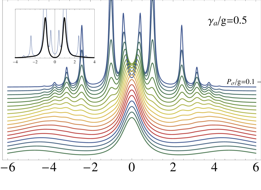
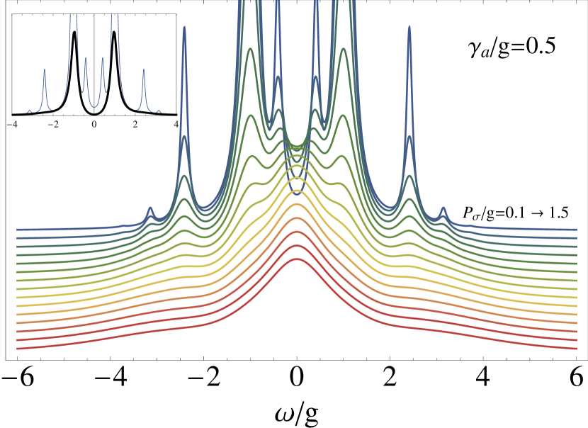
Figure 9: (Color online) Approximated spectra of emission, Eq. (IV.1), as pumping is increased and the system undergoes the quantum-to-classical transition. The plots correspond to two different cavity lifetimes ($\gamma_{a}=0.1g$ and $0.5g$). Parameters, not specified in the plots, are $P_{a}=\gamma_{\sigma}=\gamma_{\phi}=\Delta=0$. In inset, the comparison between the approximated-analytical (thin blue) and exact-numerical (thick black) spectra for the lowest pump $P_{\sigma}=0.1g$. Although the approximation breaks in the quantum regime, it shows how the Mollow triplet is formed.

In Fig. 9, we see two examples of spectra computed as in Eq. (IV.1) with $\mathrm{T}[n]$ taken as Poissonian. The first case, with $\gamma_{a}=0.1g$, corresponds to a very good cavity well in the strong coupling regime with the emitter, such as is realized in circuit QED. The second case, with $\gamma_{a}=0.5g$, corresponds to a less favourable situation representative of the state of the art of systems such as quantum dots in microcavities Ohta et al. (2011). In both plots, the pump increases from the top to the bottom curves and features the quantum to classical crossover. The transitions between the Jaynes-Cummings rungs are first resolved individually, at low pumping, and then merge into a Mollow triplet. The approximated spectrum of emission differs from the numerical exact result at low pumpings, since the assumption of much larger pumping than decay does not apply here. The regime of validity for our approximated spectrum and that for the observation of the Mollow triplet with incoherent excitation is:

$$\gamma_{a}\,,\gamma_{\sigma}\,,\gamma_{\phi}\ll g<P_{\sigma}\ll\kappa_{\sigma}\,.$$ (61)

Note that out of resonance, one must consider $g_{\mathrm{eff}}[1]$ instead of $g$ in Eq. (61). As the position of the peaks is still well approximated, however, this approximation provides an instructive and physically transparent picture of the Mollow triplet formation. We analyse these peak positions in more details in the next subsection.

IV.2 Peak positions

Let us recall the expression of the Jaynes-Cummings quadruplets positions in the spontaneous regime, in order to appreciate better the features brought by the incoherent pump del Valle et al. (2009):

$$\Omega_{\mathrm{O},\mathrm{I}}[n]=\Re\Big{[}\sqrt{g^{2}(n+1)-\left(\frac{\gamma_{a}-\gamma_{\sigma}}{4}\right)^{2}}\\ \pm\sqrt{g^{2}n-\left(\frac{\gamma_{a}-\gamma_{\sigma}}{4}\right)^{2}}\Big{]}\,.$$ (62)

These branches are plotted as thin dashed lines in Fig. 10 (only the positive frequency ones) as a function of their decoherence rate $\Gamma=\gamma_{a}-\gamma_{\sigma}$. They can be exactly mapped with transitions between rungs in the dissipative Jaynes-Cummings ladder, exhibiting three regimes depending on their splittings: (a) at low decoherence, both rungs—initial and final—are split (in the strong coupling regime) and we have four peaks (two shown in the figure). (b) When the lower rung enters weak coupling and recovers the bare modes, only two transitions (one in the figure) can be seen from the upper, still split, rung. (c) At large decoherence, none of the rungs are split and all transitions are at the origin.

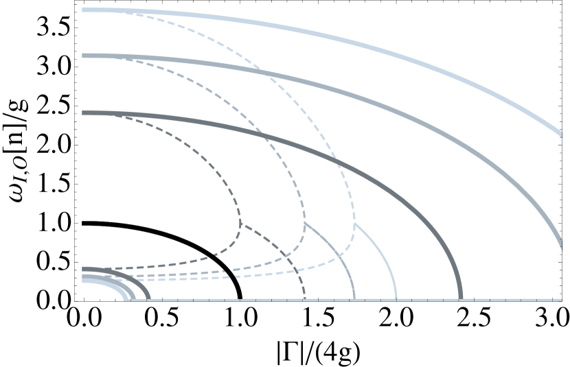
Figure 10: Transition energies (positions of the spectral peaks) as a function of decoherence $|\Gamma|/(4g)$ from rungs $n=1,2,3,4$ (from dark to light lines) for two cases: spontaneous emission ($\Gamma=\gamma_{a}-\gamma_{\sigma}$, Eq. (62), thin dashed lines) and in the presence of pumping ($\Gamma=\Gamma_{\sigma}-\gamma_{\phi}$, Eq. (60a) thick lines). The line starting at $\omega=g$ corresponds to the linear regime or first-rung-to-vacuum transition ($\Re(R_{0})$, thick black line) and is common to both cases. The curves starting above (resp. below) 1 correspond to the outer (inner) transitions.

In the same Fig. 10, we have plotted with thick lines the positions in the presence of pumping, Eq. (60a), as a function of the corresponding decoherence rate, $\Gamma=P_{\sigma}+\gamma_{\sigma}$. The positions, paired around the centre (still only the positive half is shown), also depend on the rung. In the linear regime, $n=0$, these are simply the two Rabi transitions $\pm\Re(R_{0})$, with the same structure as two coupled harmonic oscillators or the spontaneous regime that we have just described. However, for $n>0$ outer and inner peaks have an interesting nontrivial behaviour. The inner peaks close at low $\Gamma$, before the Rabi transitions do, forming, in the lasing or classical regime ($n_{a}\gg 1$), the central peak of the Mollow triplet. The outer peaks close much after the corresponding Rabi peaks do, grouping to form the two side bands of the Mollow triplet with $\omega_{\mathrm{O}}[n]\approx\Re\sqrt{4ng^{2}-\Big{(}\Gamma_{\sigma}/4\Big{)}^{2}}$ (see Fig. 9).

In the presence of pumping, it is no longer possible to map exactly the position of the peaks composing the spectra with transitions from the Jaynes-Cummings ladder. The effect of the incoherent pump, before being so strong to close the dressed state splitting of the Jaynes-Cummings rungs, is to make it homogeneous throughout the ladder. Then, the inner peaks do not close because the rungs enter the weak coupling regime but rather because the transitions coincide with the cavity frequency. In any case, the Jaynes-Cummings structure is very much distorted and the transitions between its rungs very much mixed, in such a way that it is no longer possible to reconstruct the ladder. Furthermore, in our derivation of Eq. (54) we have neglected the interplay between the cavity and emitter dynamics (by assuming them to have very different time scales) and, therefore, Fig. 9 shows the isolated effect of the incoherent pump in contrast with the complex features we observed in Fig. 8.

IV.3 Elastic scattering $E^{c}$

It is possible to give the general expression (with detuning, dephasing and decay) for the elastic scattering contribution to the spectra, for both emitter and cavity emission:

$$\Re(E^{\sigma})=\frac{4g}{\Gamma_{\sigma}+\gamma_{\phi}}\sum_{n=0}^{\infty}$$ (63a)

$$\frac{\gamma_{\sigma}(\kappa_{a}+2\Gamma_{\sigma})\sqrt{1+n}\mathrm{q}_{\mathrm{i}}[n+1]+P_{\sigma}(\kappa_{a}-2\Gamma_{\sigma})\sqrt{n}\mathrm{q}_{\mathrm{i}}[n]}{\kappa_{a}^{2}\Big{[}1+(\frac{2\Delta}{\Gamma_{\sigma}+\gamma_{\phi}})^{2}\Big{]}+4\Gamma_{\sigma}^{2}+4\Gamma_{\sigma}\kappa_{a}(2n+1)}\,,$$

$$\Re(E^{a})=\sum_{n=0}^{\infty}\frac{2}{\kappa_{a}^{2}\Big{[}1+(\frac{2\Delta}{\Gamma_{\sigma}+\gamma_{\phi}})^{2}\Big{]}+4\Gamma_{\sigma}^{2}+4\Gamma_{\sigma}\kappa_{a}(2n+1)}$$

$$\times\Big{\{}\gamma_{\sigma}(\kappa_{a}(4n+1)+2\Gamma_{\sigma})(1+n)\mathrm{T}[n+1]$$

$$+P_{\sigma}(\kappa_{a}(4n+3)+2\Gamma_{\sigma})n\mathrm{T}[n]\Big{\}}\,.$$ (63b)

Note that $\Re(E^{a})>0$ in all cases, while $\Re(E^{\sigma})$ can be negative, as we pointed out in the discussion of Fig. 7. The expressions (63) support our qualitative discussions. In the cavity emission, the scattering peak is simply the direct emission of photons through the cavity mode and therefore, is always positive. For the emitter, however, these coherent cavity photons must “convert” into material excitations before being emitted, which implies the possibility of interferences that can be positive or negative. This change of sign is even more clear when $\gamma_{\sigma}=0$ where $E^{\sigma}<0$ if $P_{\sigma}<\sqrt{2}g$. At low pumping, this carves a “hole” in the spectra pinned at the cavity frequency. For $P_{\sigma}>\sqrt{2}g$, the delta peak is positive. In the case of the cavity, most of the emission comes from it, and not the de-excitation of the dressed states, that is, from the photons that undergo an efficient interaction with the emitter.

When the two-level system is not sufficiently populated/inverted (at low $P_{\sigma}$), the cavity has a smaller elastic scattering contribution. The emitter sees an interference hole being carved in its spectrum, reminiscent of a Fano resonance. The emitter represents an efficient pumping for the cavity in a linear way. As we already mentioned, the cavity is sucking the cavity photons (at $\omega_{a}$) out of the emitter. Although at very low pumping ($P_{\sigma}\approx\gamma_{a}$) these approximations are not valid (a delta function weighted negatively means a negative spectrum) and do not provide a quantitative agreement with the numerical results, they are interesting to understand the qualitative features that are obtained numerically.

When the two-level system is saturated in the self-quenching regime (at high $P_{\sigma}$), it is mainly in its excited state. The cavity spectrum tends towards the bare cavity emission (thermal regime). In the exact solution, this is a Lorentzian with the cavity linewidth $\gamma_{a}$. In our approximated solution, the cavity bare emission is a delta function and the two-level system emission loses completely the elastic scattering component because there is weak interaction with the cavity which provides it.

In the lasing region, $1<P_{\sigma}<20g$, the triplet appears in both channels of emission: cavity and emitter. The emitter grows some small positive elastic scattering component on top of the triplet, as a collateral effect from the strong interaction with the cavity (proportional to $\mathrm{q}_{\mathrm{i}}[n]$).

IV.4 Semiclassical approximation

In the lasing regime, where the $n$ and $n+1$ rungs that are close to $n_{a}$ (having $n_{a}\gg 1$) have similar splittings and the cavity field becomes Poissonian (coherent), simple expressions—in regard to the complexity of the underlying machinery to obtain them—arise for the spectra of emission del Valle and Laussy (2010). The variable $n$ becomes continuous as compared to the large intensity $n_{a}$ and, given that the distribution is Poissonian (peaked at the mean value), we can consider only the case $n=n_{a}$ in Eq. (IV.1). The integral over the distribution $\mathrm{T}[n]$ simplifies to 1. In this regime, the inner peaks have collapsed into the centre while the outer remain splitted. Substituting $n_{a}$ (and $n_{\sigma}$ for the normalization) from Eq. (IV.1), we obtain the final expression for the emitter spectrum:

$$S_{\sigma}(\omega)=\Big{(}\frac{2P_{\sigma}}{\Gamma_{\sigma}+\gamma_{\phi}+\kappa_{\sigma}}-\frac{\Gamma_{\sigma}}{\kappa_{\sigma}}\Big{)}\delta(\omega)+\frac{1}{2\pi}\frac{\frac{\Gamma_{\sigma}+\gamma_{\phi}}{2}}{\big{(}\frac{\Gamma_{\sigma}+\gamma_{\phi}}{2}\big{)}^{2}+\omega^{2}}\\ +\frac{1}{(\Gamma_{\sigma}+\gamma_{\phi}+\kappa_{\sigma})[(-2P_{\sigma}+\Gamma_{\sigma})^{2}\kappa_{\sigma}^{2}+((3\Gamma_{\sigma}+\gamma_{\phi})^{2}+4(\Gamma_{\sigma}-2P_{\sigma})\kappa_{\sigma})\omega^{2}+4\omega^{4}]}\Big{\{}-4P_{\sigma}^{2}\kappa_{\sigma}(3\Gamma_{\sigma}+\gamma_{\phi}+\kappa_{\sigma})\\ +2P_{\sigma}\Gamma_{\sigma}[3\Gamma_{\sigma}^{2}+4\Gamma_{\sigma}(\gamma_{\phi}+2\kappa_{\sigma})+(\gamma_{\phi}+\kappa_{\sigma})(\gamma_{\phi}+3\kappa_{\sigma})]+4P_{\sigma}\kappa_{\sigma}\omega^{2}-(\Gamma_{\sigma}+\gamma_{\phi}+\kappa_{\sigma})[\Gamma_{\sigma}^{2}(3\Gamma_{\sigma}+\gamma_{\phi}+2\kappa_{\sigma})+(\Gamma_{\sigma}-\gamma_{\phi})\omega^{2}]\Big{\}}\,.$$ (64)

Similarly to the coherent excitation case, it is composed of an elastic scattering term (delta peak), a central peak (a Lorentzian peak with FWHM $\Gamma_{\sigma}+\gamma_{\phi}$) and two side bands. When splitted, these have a FWHM $(3\Gamma_{\sigma}+\gamma_{\phi})/2$ and positions given by $\omega_{\mathrm{O}}[n_{a}]\approx\Re(R_{\mathrm{O}})$ where

$$R_{\mathrm{O}}=\sqrt{\frac{(2P_{\sigma}-\Gamma_{\sigma})\kappa_{\sigma}}{2}-\big{(}\frac{\Gamma_{\sigma}+\gamma_{\phi}}{4}\big{)}^{2}}\,.$$ (65)

This is the Mollow splitting in the case of incoherent excitation, analogous to $R_{\mathrm{L}}$ in Eq. (11). It is plotted in Fig. 11. Contrary to the laser excitation, this splitting can now close due to the pumping intensity $P_{\sigma}$. In Fig. 11, we show the domains where the Mollow triplet is clearly resolved. This naturally requires that the system is able to enter the regime of lasing in strong-coupling, which starts at figures of about $\gamma_{a}/g\approx 0.1$. This is the case shown in the Figure, where we compare the Mollow splitting, Eq. (11), with the observed splitting, represented as the shaded area which is delimited by the maximum (upper boundary, solid) and the neck (lower boundary, dashed) of a side peak. When the Mollow splitting is maximum, decoherence has however broadened so much the satellite peaks that no triplet is observable anymore.

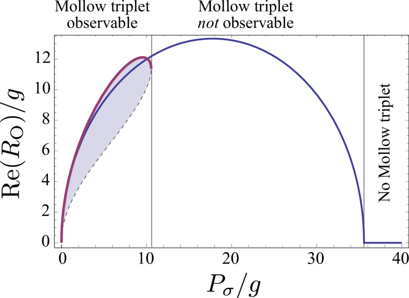
Figure 11: (Color online) Comparison between the position of the side peaks ($\Re(R_{\mathrm{O}})$, in solid blue) and those observed in the emitter spectrum ($\omega_{\mathrm{obs}}$, in solid purple, above the filling), as a function of pumping. In dashed is shown the neck of the side peak so that the filled area delimits approximately its half-width.

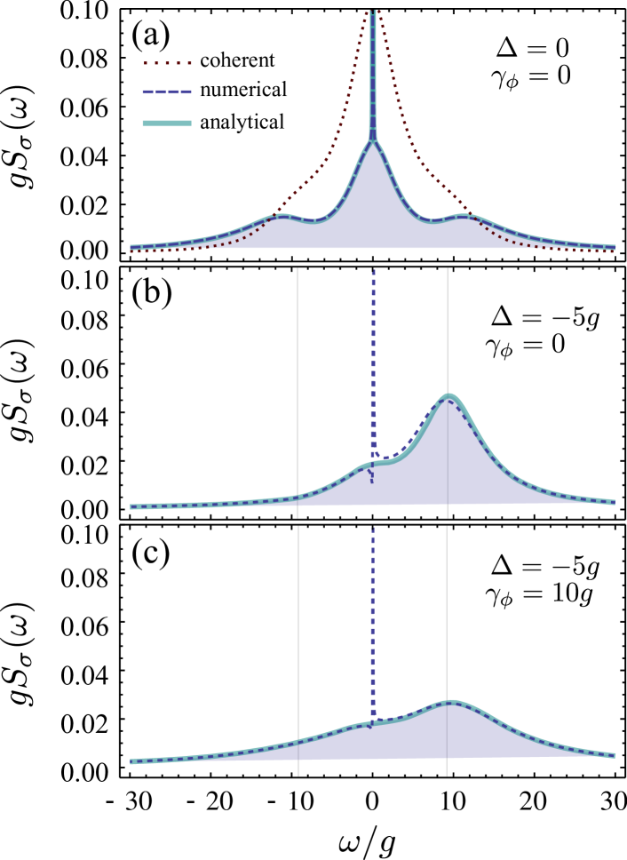
Figure 12: (Colour online) Mollow triplet in the direct PL spectra from the emitter, $S_{\sigma}(\omega)$ for $\gamma_{a}=0.1g$, $P_{a}=0$, $\gamma_{\sigma}=0.00334$ and $P_{\sigma}=7g$ ($n_{a}\approx 11.6$ and $n_{\sigma}\approx 0.53$), for various configurations of detuning and dephasing. The exact numerical results are plotted with a dark-blue dashed line, overlapping almost exactly our analytical formula, in light-blue solid. The coherent scattering peak is featured in the analytical solution in (a) while only the incoherent spectrum is shown in (b) and (c). The dotted line in (a) represents the Mollow triplet obtained under coherent excitation, with a laser intensity equivalent to the cavity occupation in the incoherent case, that is, for $\Omega_{\mathrm{L}}=\sqrt{n_{a}}g$ and also an equivalent emitter broadening, $\gamma_{\sigma}\rightarrow\gamma_{\sigma}+P_{\sigma}$. The two types of Mollow lineshapes are clearly different even though their peak positions and broadening are equal. Also, as compared to the coherent excitation case, the Mollow triplet under incoherent pumping is a resonant structure that becomes strongly asymmetric with detuning.

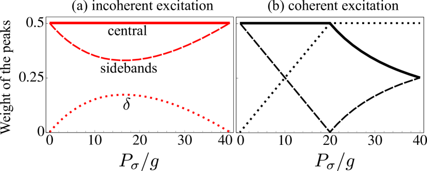
Figure 13: Contributions to the Mollow triplet under (a) incoherent and (b) coherent excitation for the three types of peaks: the central Lorentzian peak (constant at $1/2$, solid line), the side bands (dashed) and the elastic scattering peak (dotted). The parameters are chosen so that the two Mollow triplets can be compared on equal grounds, as explained in the text, for $\gamma_{a}=0.1g$, $P_{a}=0$, $\gamma_{\sigma}=\gamma_{\phi}=0$ and $\Delta=0$.

Applying the same procedure, for the cavity emission we have $S_{a}(\omega)=\delta(\omega)$, that is, a purely elastic spectrum with negligible linewidth. A more accurate approximation to the FWHM of the elastic peaks in this regime, which reproduces the typical lasing cavity line narrowing, is given by the broadening $\gamma_{\mathrm{L}}$:

$$\gamma_{\mathrm{L}}=2g^{2}\gamma_{a}/P_{\sigma}^{2}$$ (66)

as derived by Poddubny et al. Poddubny et al. (2010).

In Fig. 12, we show the excellent agreement between the analytical approximation (in dashed lines) and the exact numerical computation (solid lines). In Fig. 12(a), the case of resonance—the one of most interest—is where the Mollow triplet is best observed. Its analytical expression is given by Eq. (64), where we also include the scattering peak, (both as a result of the numerical procedure and approximated by Eq. (66)) seen as a very sharp line, which we have truncated in the plot, as it extends more than one hundred times higher than is shown. In Fig. 12(a), we also provide further evidence that the Mollow triplet formed under incoherent pumping is of a different nature than that formed under coherent excitation del Valle and Laussy (2010), by superimposing the coherent excitation Mollow triplet (dotted line). We take $\Omega_{\mathrm{L}}\rightarrow\sqrt{n_{a}}g$ and $\gamma_{\sigma}\rightarrow\gamma_{\sigma}+P_{\sigma}$ to compare both expressions on equal grounds (both lineshapes remain dissimilar even when parameters are left completely free). This substitution makes both types of triplet share the same position and broadening for their three peaks. However their relative weight is different, as shown in Fig. 13. These strong qualitative departures result in the striking differences between the final spectra, although the peaks have identical characteristic if taken in isolation.

When the system is not at resonance, in sharp contrast with the conventional Mollow triplet that retained its qualitative features (cf. Fig. 1), the Mollow triplet under incoherent pumping becomes strongly asymmetric, as it recovers the scenario of an anticrossing of two modes. The out-of resonance case is studied in details in Fig. 14. Whereas both detuning and dephasing were needed to break the symmetry of the conventional Mollow triplet, the one formed under incoherent pumping is lost by detuning alone, pumping playing already the role of dephasing. Dephasing has otherwise the expected effect of smearing out and broadening the spectral features. Analytical results can also be given for the non-resonant case when $\Delta\neq 0$, but, as for the conventional Mollow, they are too long to be reasonably written down. We plot it on top of the numerical solution in Figs. 12(b) and (c) where one can see the semiclassical approximation is excellent there as well.

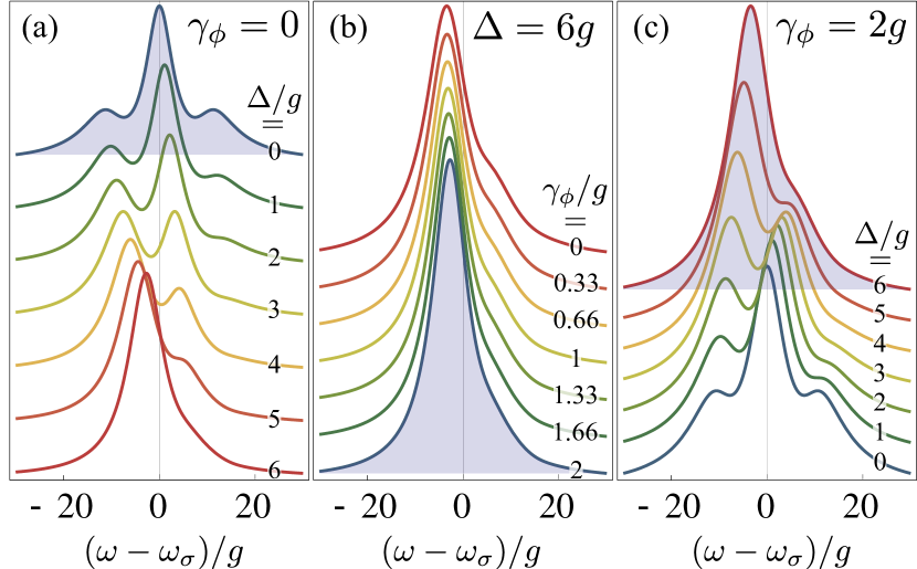
Figure 14: Counterpart of Fig. 1 for the Mollow triplet under incoherent excitation. In contrast to the coherent excitation case, detuning alone breaks the Mollow triplet. Parameters are $\gamma_{a}/g=0.1$, $\gamma_{\sigma}/g=0.01$, $P_{a}=0$ and $P_{\sigma}/g=7$.

V Summary and Outlooks

We investigated the steady states of the Jaynes–Cummings Hamiltonian established under the interplay of decay and incoherent pumping (of the emitter), including pure dephasing and detuning for wider generality. This is the simplest and most fundamental realization of a fully quantized system, realized with atoms, quantum dots or superconducting qubits in a cavity. We identify five regimes through semi-analytical and approximated solutions, all confronted to exact numerical solutions. These are: $i$ the linear quantum regime, $ii$ the nonlinear quantum regime, $iii$ the nonlinear classical regime, or lasing regime, $iv$ the self-quenching regime and $v$ the thermal regime. We provided closed-form analytical expressions that account for most of theses regimes and a simple numerical procedure (solving a set of two coupled nonlinear equations) that afford an excellent description over the entire range of excitation and all the five regimes that we have outlined. This also allows a transparent reading of the physics involved, namely, the first regime involves the lowest rung of the Jaynes–Cummings ladder only and corresponds to spontaneous emission. A linear-model (two coupled oscillators) and a truncated Jaynes–Cummings model offer two complementary views of this regime. The quantum regime is the one where the system starts to climb the ladder, requiring a full record of all the quantum correlators involved. This is therefore the most complicated regime from the point of view of the amount of information required to describe it, since no good approximation can synthesize the dynamics of a few quanta. In very good systems, this manifests spectrally in a complex structure of peaks at anharmonic frequencies. As pumping is further increased, lasing ensues which brings back the system to a simple level of description in a semiclassical approximation. A single narrowing line in the cavity or a variation of the Mollow triplet for the emitter describe accurately the system. In the fully quantized picture, lasing appears as a condensate of dressed states, with a complex pattern that however does not manifest in the observable, showing a breakdown of the quantized picture in favour of a classical description.

The Jaynes–Cummings model that arose as a challenge for full-field quantization Stroud (2004) remains to this day a proficient source of theoretical and experimental investigations into the quantum realm. The realization in the laboratory of the nontrivial quantum physics that it covers will shed light on foremost issues such as the quantum to classical crossover, emergence of coherence, lasing and quantum nonlinearities. A solid understanding of the various regimes it realizes may also lead to useful devices and applications, from single-photon sources to low-threshold lasers.

Appendix A Quantum regression formula for coherent excitation

Two-time correlators of the type $\langle{\sigma^{\dagger}}(0)\sigma(\tau)\rangle$ can be computed by means of the quantum regression formula del Valle et al. (2009). Once we find the set of operators $C_{\{m,n\}}={{\sigma^{\dagger}}}^{m}\sigma^{n}$ (with $m$, $n\in\{0,1\}$) and the regression matrix $M_{\begin{subarray}{c}mn\\ m^{\prime}n^{\prime}\end{subarray}}$ that satisfy $\mathrm{Tr}{[C_{\{m,n\}}\mathcal{L}O]}=\sum_{\{m^{\prime}n^{\prime}\}}M_{\begin{subarray}{c}mn\\ m^{\prime}n^{\prime}\end{subarray}}\mathrm{Tr}{[C_{\{m^{\prime},n^{\prime}\}}O]}$ for a general operator $O$, then the equations of motion for the two-time correlators ($\tau\geq 0$) in the steady state ($t=0$) read:

$$\partial_{\tau}\langle O(0)C_{\{m,n\}}(\tau)\rangle=\sum_{\{m^{\prime}n^{\prime}\}}M_{\begin{subarray}{c}mn\\ m^{\prime}n^{\prime}\end{subarray}}\langle O(0)C_{\{m^{\prime},n^{\prime}\}}(\tau)\rangle\,.$$ (67)

The corresponding regression matrix $M$ is given, in the case of a coherent and classical excitation of the emitter, as explained in section II, by:

$$M_{\begin{subarray}{c}mn\\ mn\end{subarray}}=i\Delta_{L}(m-n)-\frac{\gamma_{\sigma}}{2}(m+n)-\frac{\gamma_{\phi}}{2}(m-n)^{2}\,,$$ (68a)

$$M_{\begin{subarray}{c}mn\\ 1-m,n\end{subarray}}=i\Omega_{\mathrm{L}}[m+2n(1-m)]\,,$$ (68b)

$$M_{\begin{subarray}{c}mn\\ m,1-n\end{subarray}}=-i\Omega_{\mathrm{L}}[n+2m(1-n)]\,.$$ (68c)

and zero everywhere else. We concentrate on computing $g_{1}^{(1)}$, which corresponds to setting $O={\sigma^{\dagger}}$ and having $\{m,n\}=\{0,1\}$ in Eq. (67). We obtain the following differential equation:

$$\partial_{\tau}\mathbf{v}_{L}(\tau)=-\mathbf{M}_{L}\mathbf{v}_{L}(\tau)+\mathbf{A}_{L}\langle{\sigma^{\dagger}}\rangle\,,$$ (69)

where

$$\mathbf{v}_{L}(\tau)=\begin{pmatrix}\langle{\sigma^{\dagger}}(0)\sigma(\tau)\rangle\\ \langle{\sigma^{\dagger}}(0){\sigma^{\dagger}}(\tau)\rangle\\ \langle{\sigma^{\dagger}}(0){\sigma^{\dagger}}\sigma(\tau)\rangle\end{pmatrix}\,,\quad\mathbf{A}_{L}=i\Omega_{\mathrm{L}}\begin{pmatrix}-1\\ 1\\ 0\end{pmatrix}$$ (70)

and

$$\mathbf{M}_{L}=\begin{pmatrix}-i\Delta_{L}+\frac{\gamma_{\sigma}+\gamma_{\phi}}{2}&0&-2i\Omega_{\mathrm{L}}\\ 0&i\Delta_{L}+\frac{\gamma_{\sigma}+\gamma_{\phi}}{2}&2i\Omega_{\mathrm{L}}\\ -i\Omega_{\mathrm{L}}&i\Omega_{\mathrm{L}}&\gamma_{\sigma}\end{pmatrix}\,.$$ (71)

The solution is

$$\mathbf{v}_{L}(\tau)=e^{-\mathbf{M}_{L}\tau}[\mathbf{v}_{L}(0)-\mathbf{M}_{L}^{-1}\mathbf{A}_{L}\langle{\sigma^{\dagger}}\rangle]+\mathbf{M}_{L}^{-1}\mathbf{A}_{L}\langle{\sigma^{\dagger}}\rangle\,,$$ (72)

in terms of the steady steady values $\langle{\sigma^{\dagger}}\rangle$ and $\mathbf{v}_{L}(0)=[\langle{\sigma^{\dagger}}\sigma\rangle,0,0]$ (initial condition of Eq. (70)). We also need, therefore, to compute the steady state of the system,

$$\mathbf{u}_{L}=\begin{pmatrix}\langle\sigma\rangle\\ \langle{\sigma^{\dagger}}\rangle\\ \langle{\sigma^{\dagger}}\sigma\rangle\end{pmatrix}\,,$$ (73)

which can be done, again, by means of the general formula in Eq. (67). This time we take $O=1$ and  $\{m,n\}=\{0,1\}$, $\{1,0\}$, $\{1,1\}$ and find the equation:

$$\partial_{t}\mathbf{u}_{L}=0=-\mathbf{M}_{L}\mathbf{u}_{L}+\mathbf{A}_{L}\,.$$ (74)

The solution is $\mathbf{u}_{L}=\mathbf{M}_{L}^{-1}\mathbf{A}_{L}$. It allows us to simplify Eq. (72) further as

$$\mathbf{v}_{L}(\tau)=e^{-\mathbf{M}_{L}\tau}[\mathbf{v}_{L}(0)-\mathbf{u}_{L}\langle{\sigma^{\dagger}}\rangle]+\mathbf{u}_{L}\langle{\sigma^{\dagger}}\rangle\,,$$ (75)

The final explicit solutions for the mean values and correlators of interest are presented in the main text.

Appendix B Derivation of the field correlators and density matrix

The equations of motion of the correlators in Eq. (17) can be derived from the master equation (16) by simply applying the general formula $\langle O\rangle=\mathrm{Tr}{(O\rho)}$ or from the rules given by the quantum regression formula del Valle et al. (2009):

$$\partial_{t}N_{a}[n]=-n\Gamma_{a}N_{a}[n]+n^{2}P_{a}N_{a}[n-1]$$ (76a)

$$+2gnN^{i}_{a\sigma}[n]\,,$$

$$\partial_{t}N_{\sigma}[n]=-\big{[}\Gamma_{a}(n-1)+\Gamma_{\sigma}\big{]}N_{\sigma}[n]$$ (76b)

$$+P_{a}(n-1)^{2}N_{\sigma}[n-1]+P_{\sigma}N_{a}[n-1]-2gN^{i}_{a\sigma}[n]\,,$$

$$\partial_{t}N^{i}_{a\sigma}[n]=-\Big{[}\frac{\Gamma_{a}}{2}(2n-1)+\frac{\Gamma_{\sigma}+\gamma_{\phi}}{2}\Big{]}N^{i}_{a\sigma}[n]$$ (76c)

$$+P_{a}n(n-1)N^{i}_{a\sigma}[n-1]+\Delta N^{r}_{a\sigma}[n]$$

$$+g(2N_{\sigma}[n+1]+nN_{\sigma}[n]-N_{a}[n])\,,$$

$$\partial_{t}N^{r}_{a\sigma}[n]=-\Big{[}\frac{\Gamma_{a}}{2}(2n-1)+\frac{\Gamma_{\sigma}+\gamma_{\phi}}{2}\Big{]}N^{r}_{a\sigma}[n]$$ (76d)

$$+P_{a}n(n-1)N^{r}_{a\sigma}[n-1]-\Delta N^{i}_{a\sigma}[n]\,,$$

with $n\geq 1$ and also $N_{a}[0]=1$. In the steady state, with $P_{a}=0$, one can further simplify these equations and write $N_{a\sigma}[n]$ and $N_{\sigma}[n]$ in terms of $N_{a}[n]$ to obtain Eqs. (19).

The master equation (16) can also be rewritten in terms of the density matrix elements in Eq. (45) as:

$$\partial_{t}\mathrm{p}_{0}[n]=-\big{[}(\gamma_{a}+P_{a})n+P_{a}\big{]}\mathrm{p}_{0}[n]$$ (77a)

$$+\gamma_{a}(n+1)\mathrm{p}_{0}[n+1]+P_{a}n\mathrm{p}_{0}[n-1]$$

$$-P_{\sigma}\mathrm{p}_{0}[n]+\gamma_{\sigma}\mathrm{p}_{1}[n]-2g\sqrt{n}\mathrm{q}_{\mathrm{i}}[n]\,,$$

$$\partial_{t}\mathrm{p}_{1}[n]=-\big{[}(\gamma_{a}+P_{a})n+P_{a}\big{]}\mathrm{p}_{1}[n]$$ (77b)

$$+\gamma_{a}(n+1)\mathrm{p}_{1}[n+1]+P_{a}n\mathrm{p}_{1}[n-1]$$

$$-\gamma_{\sigma}\mathrm{p}_{1}[n]+P_{\sigma}\mathrm{p}_{0}[n]+2g\sqrt{n+1}\mathrm{q}_{\mathrm{i}}[n+1]\,,$$

$$\partial_{t}\mathrm{q}_{\mathrm{i}}[n]=-\Big{[}(\gamma_{a}+P_{a})n-\frac{\Gamma_{a}}{2}\Big{]}\mathrm{q}_{\mathrm{i}}[n]$$ (77c)

$$+\gamma_{a}\sqrt{(n+1)n}\mathrm{q}_{\mathrm{i}}[n+1]+P_{a}\sqrt{(n-1)n}\mathrm{q}_{\mathrm{i}}[n-1]$$

$$-\frac{\Gamma_{\sigma}+\gamma_{\phi}}{2}\mathrm{q}_{\mathrm{i}}[n]+g\sqrt{n}(\mathrm{p}_{0}[n]-\mathrm{p}_{1}[n-1])-\Delta\,\mathrm{q}_{\mathrm{r}}[n]\,,$$

$$\partial_{t}\mathrm{q}_{\mathrm{r}}[n]=-\Big{[}(\gamma_{a}+P_{a})n-\frac{\Gamma_{a}}{2}\Big{]}\mathrm{q}_{\mathrm{r}}[n]$$ (77d)

$$+\gamma_{a}\sqrt{(n+1)n}\mathrm{q}_{\mathrm{r}}[n+1]+P_{a}\sqrt{(n-1)n}\mathrm{q}_{\mathrm{r}}[n-1]$$

$$-\frac{\Gamma_{\sigma}+\gamma_{\phi}}{2}\mathrm{q}_{\mathrm{r}}[n]+\Delta\,\mathrm{q}_{\mathrm{i}}[n]\,.$$

At resonance, the real part of the coherence distribution, $\mathrm{q}_{\mathrm{r}}$, gets decoupled and vanishes in the steady state. As a result, only Eqs. (77)–(77) need to be solved. When $g$ vanishes, $\mathrm{q}_{\mathrm{i}}$ does not couple the two modes anymore, and their statistics become thermal, like in the boson case. Through the off-diagonal elements $\mathrm{q}_{\mathrm{i}}$, the photon density matrix can vary between Poissonian, thermal (superpoissonian) and subpoissonian distributions.

In order to solve these equations in the steady state, we neglect the photonic dynamics (as explained in the main text) and further substitute $\mathrm{q}_{\mathrm{r}}[n]=[2\Delta/(\Gamma_{\sigma}+\gamma_{\phi})]\mathrm{q}_{\mathrm{i}}[n]$ in the equation for $\mathrm{q}_{\mathrm{i}}$, and write everywhere $\mathrm{p}_{0}[n]$ as $\mathrm{T}[n]-\mathrm{p}_{1}[n]$ and $\mathrm{p}_{1}[n+1]$ as $\mathrm{T}[n+1]-\mathrm{p}_{0}[n+1]$, so that $\mathrm{q}_{\mathrm{r}}[n]$, $\mathrm{p}_{0}[n]$, $\mathrm{p}_{1}[n+1]$ do not appear explicitly in the remaining three equations. Then, the equations read in matricial form:

$$\partial_{t}\mathbf{u}_{0}[n]=-\mathbf{M}_{0}[n]\mathbf{u}_{0}[n]+\mathbf{A}_{0}[n]$$ (78)

with:

$$\mathbf{u}_{0}[n]=\begin{pmatrix}\mathrm{p}_{0}[n+1]\\ \mathrm{p}_{1}[n]\\ \mathrm{q}_{\mathrm{i}}[n+1]\end{pmatrix}\,,\quad\mathbf{A}_{0}[n]=\begin{pmatrix}\gamma_{\sigma}\mathrm{T}[n+1]\\ P_{\sigma}\mathrm{T}[n]\\ 0\end{pmatrix}\,,\\ \mathbf{M}_{0}[n]=\begin{pmatrix}\Gamma_{\sigma}&0&2g\sqrt{n+1}\\ 0&\Gamma_{\sigma}&-2g\sqrt{n+1}\\ -g\sqrt{n+1}&g\sqrt{n+1}&\frac{\Gamma_{\sigma}+\gamma_{\phi}}{2}+\frac{2\Delta^{2}}{\Gamma_{\sigma}+\gamma_{\phi}}\end{pmatrix}\,.$$ (79)

The solution in the steady state is $\mathbf{u}_{0}[n]=(\mathbf{M}_{0}[n])^{-1}\mathbf{A}_{0}[n]$ which gives the result of the text, Eq. (47). Note that this solution is only exact in the case $\gamma_{a}=P_{a}=0$.

Appendix C Perturbative regime of interaction in the limit of weak coupling

Eq. (20) can be solved exactly as a series Taylor expansion on the pumping $P_{\sigma}$. For this, we rewrite Eq. (20) in terms of the fraction $F[n]=N_{a}[n+1]/N_{a}[n]=n_{a}g^{(n+1)}/g^{(n)}$ (for $n>1$):

$$F[n-1](F[n]+\frac{B_{n}}{A_{n}})=\frac{C_{n}}{A_{n}}$$ (80)

where

$$A_{n}= \frac{2\gamma_{a}}{\Gamma_{\sigma}+n\gamma_{a}}\,,$$ (81a)

$$B_{n}= \frac{1}{C_{\mathrm{eff}}[n]}+\frac{n\gamma_{a}}{\Gamma_{\sigma}+(n-1)\gamma_{a}}-\frac{2P_{\sigma}}{\Gamma_{\sigma}+n\gamma_{a}}+1\,,$$ (81b)

$$C_{n}= \frac{nP_{\sigma}}{\Gamma_{\sigma}+(n-1)\gamma_{a}}\,.$$ (81c)

All quantities can be expanded, or assumed to have a solution in the case of $F[n]$, in power series of $P_{\sigma}$:

$$\frac{B_{n}}{A_{n}}=\sum_{k=0}^{\infty}\alpha_{k}[n]P_{\sigma}^{k}\,,\quad\frac{C_{n}}{A_{n}}=\sum_{k=0}^{\infty}\beta_{k}[n]P_{\sigma}^{k}\,,$$ (82a)

$$F[n]=\sum_{k=0}^{\infty}f_{k}[n]P_{\sigma}^{k}\,.$$ (82b)

A key feature of this expansion is that $\beta_{0}[n]=0$ and $f_{0}[n]=0$ for all $n$ (we recall the linear behaviour of $n_{a}$ at low pumping). With this considerations, Eq. (80) now reads

$$\sum_{q=1}^{\infty}\sum_{k=1}^{\infty}f_{q}[n-1](f_{k}[n]+\alpha_{k}[n])P_{\sigma}^{k+q}=\sum_{t=1}^{\infty}\beta_{t}[n]P_{\sigma}^{t}\,.$$ (83)

We further change the sum index $q$, on the left hand side of the equation, for $t=q+k$, so that we can get rid of it and of the pump dependence:

$$\sum_{k=1}^{t}f_{t-k}[n-1](f_{k}[n]+\alpha_{k}[n])P_{\sigma}^{k+q}=\beta_{t}[n]\,.$$ (84)

The exact solution can be found exactly and recurrently as:

$$f_{1}[n]=\frac{\beta_{1}[n+1]}{\alpha_{0}[n+1]}\,,$$ (85a)

$$f_{2}[n]=\frac{\beta_{2}[n+1]-f_{1}[n](f_{1}[n+1]+\alpha_{1}[n+1])}{\alpha_{0}[n+1]}\,,$$ (85b)

$$\ldots\quad$$

$$f_{t}[n]=\frac{\beta_{t}[n+1]-f_{t-1}[n]\sum_{k=1}^{t-1}(f_{k}[n+1]+\alpha_{k}[n+1])}{\alpha_{0}[n+1]}\,.$$ (85c)

This method is only useful in practical terms when the effect of the coupling is perturbative, that is, at very low pumping or in the weak coupling regime, where only a few terms of the expansion are needed. Otherwise, in order to reproduce non perturbative effects such as the transition into lasing, the sum should be performed to all orders of $P_{\sigma}$, which might not be practical numerically.

Appendix D Derivation of the two-time correlators

We can obtain the elements $\rho^{c}_{k;l}(\tau)$ needed to compute the two-time correlators in Eq. (49), in an equivalent way as $\rho_{[k;l]}$, as they follow the same master equation Mølmer (1996): $\partial_{t}\rho_{[k;l]}=\sum_{i,j}\mathcal{M}_{\Big{[}\begin{subarray}{c}k;l\\ i;j\end{subarray}\Big{]}}\rho_{[i;j]}$. That is, we can solve

$$\partial_{\tau}\rho^{c}_{[k;l]}(t+\tau)=\sum_{i,j}\mathcal{M}_{\Big{[}\begin{subarray}{c}k;l\\ i;j\end{subarray}\Big{]}}\rho^{c}_{[i;j]}(t+\tau)\,.$$ (86)

The initial conditions are given in terms of the steady state density matrix:

$$\rho^{c}_{[k;l]}(0)=\langle{c^{\dagger}}(\left|l\right\rangle\left\langle k\right|)(0)\rangle=\sum_{\alpha}\rho_{[k;\alpha]}\left\langle\alpha\right|{c^{\dagger}}\left|l\right\rangle\,.$$ (87)

Let us be more specific by writing the formulas for the two correlators of interest. For the emitter spectra, we have $\left\langle l_{1},l_{2}\right|\sigma\left|k_{1},k_{2}\right\rangle=\delta_{l_{1},k_{1}}\delta_{l_{2},0}\delta_{k_{2},1}$, which gives:

$$\langle{\sigma^{\dagger}}(0)\sigma(\tau)\rangle=\sum_{n=0}^{n_{max}}\rho^{\sigma}_{[n,1;n,0]}(\tau)\,.$$ (88)

For the cavity spectra, we have $\left\langle l_{1},l_{2}\right|a\left|k_{1},k_{2}\right\rangle=\sqrt{k_{1}}\delta_{l_{2},k_{2}}\delta_{l_{1},k_{1}-1}$, which gives:

$$\langle{a^{\dagger}}(0)a(\tau)\rangle=\sum_{n=0}^{n_{max}}\sum_{i=0,1}\sqrt{n}\rho^{a}_{[n,i;n-1,i]}(\tau)\,.$$ (89)

$\rho^{c}$ is obtained by solving the master Eq. (86) in both cases, but the initial conditions that follow in each case from Eq. (87), are different. For the emitter correlator, they are $\rho^{\sigma}_{[n,i;m,j]}(0)=\rho_{[n,i;m,1]}\delta_{j,0}$, while for the photon, $\rho^{a}_{[n,i;m,j]}(0)=\sqrt{m+1}\rho_{[n,i;m+1,j]}$. In the same way as when solving the steady state distributions, we write the master equation for $\rho^{c}_{[n,i;m,j]}$ only for the elements that will be different from zero during the evolution with $\tau$. We have to include all the elements that are nonzero in the initial condition plus those that are linked to them. One can check that the nonzero elements are the same for the initial conditions of both the cavity and the emitter correlators, those defined in Eq. (50). They follow the equations:

$$\partial_{\tau}S_{0}[n]=-\big{[}\frac{\gamma_{a}+P_{a}}{2}(2n-1)+P_{a}\big{]}S_{0}[n]$$ (90a)

$$+\gamma_{a}\sqrt{n(n+1})S_{0}[n+1]+P_{a}\sqrt{n(n-1)}S_{0}[n-1]$$

$$-P_{\sigma}S_{0}[n]+\gamma_{\sigma}S_{1}[n]+ig(\sqrt{n-1}V[n]-\sqrt{n}Q[n-1])\,,$$

$$\partial_{\tau}S_{1}[n]=-\big{[}\frac{\gamma_{a}+P_{a}}{2}(2n-1)+P_{a}\big{]}S_{1}[n]$$ (90b)

$$+\gamma_{a}\sqrt{n(n+1})S_{1}[n+1]+P_{a}\sqrt{n(n-1)}S_{1}[n-1]$$

$$+P_{\sigma}S_{0}[n]-\gamma_{\sigma}S_{1}[n]-ig(\sqrt{n+1}V[n+1]-\sqrt{n}Q[n])\,,$$

$$\partial_{\tau}Q[n]=-\Big{[}(\gamma_{a}+P_{a})n+P_{a}\Big{]}Q[n]$$ (90c)

$$+\gamma_{a}(n+1)Q[n+1]+P_{a}nQ[n-1]$$

$$-\Big{(}\frac{\Gamma_{\sigma}+\gamma_{\phi}}{2}-i\Delta\Big{)}Q[n]$$

$$+ig(\sqrt{n}S_{1}[n]-\sqrt{n+1}S_{0}[n+1])\,,$$

$$\partial_{\tau}V[n]=-\big{[}(\gamma_{a}+P_{a})n-\gamma_{a}\big{]}V[n]$$ (90d)

$$+\gamma_{a}\sqrt{(n-1)(n+1})V[n+1]+P_{a}\sqrt{n(n-2)}V[n-1]$$

$$-\Big{(}\frac{\Gamma_{\sigma}+\gamma_{\phi}}{2}+i\Delta\Big{)}V[n]$$

$$+ig(\sqrt{n-1}S_{0}[n]-\sqrt{n}S_{1}[n-1])\,.$$

As explained in the main text, we solve these equations by neglecting the very slow photonic dynamics. We then define the steady state and slow varying function

$$X[n]\equiv S_{0}[n](0)+S_{1}[n](0)\,,$$ (91)

and substitute $S_{0}[n]=X[n]-S_{1}[n]$ and $S_{1}[n+1]=X[n+1]-S_{0}[n+1]$, so that we can rewrite the equations in a matricial form (78):

$$\partial_{\tau}\mathbf{u}_{1}[n](\tau)=-\mathbf{M}_{1}[n]\mathbf{u}_{1}[n](\tau)+\mathbf{A}_{1}[n]$$ (92)

with:

$$\mathbf{u}_{1}[n]=\begin{pmatrix}S_{0}[n+1]\\ S_{1}[n]\\ Q[n]\\ V[n+1]\end{pmatrix}\,,\quad\mathbf{A}_{1}[n]=\begin{pmatrix}\gamma_{\sigma}X[n+1]\\ P_{\sigma}X[n]\\ 0\\ 0\end{pmatrix}\,,\\ \text{and\ }\mathbf{M}_{1}[n]=\\ \begin{pmatrix}\Gamma_{\sigma}&0&ig\sqrt{n+1}&-ig\sqrt{n}\\ 0&\Gamma_{\sigma}&-ig\sqrt{n}&ig\sqrt{n+1}\\ ig\sqrt{n+1}&-ig\sqrt{n}&\frac{\Gamma_{\sigma}+\gamma_{\phi}}{2}-i\Delta&0\\ -ig\sqrt{n}&ig\sqrt{n+1}&0&\frac{\Gamma_{\sigma}+\gamma_{\phi}}{2}+i\Delta\end{pmatrix}\,.$$ (93)

The solution in the steady state is

$$\mathbf{u}_{1}[n](\tau)=e^{-\mathbf{M}_{1}[n]\tau}\Big{(}\mathbf{u}_{1}[n](0)-(\mathbf{M}_{1}[n])^{-1}\mathbf{A}_{1}[n]\Big{)}\\ +(\mathbf{M}_{1}[n])^{-1}\mathbf{A}_{1}[n]\,.$$ (94)

For the emitter correlator, the initial condition derived from Eq. (87) reads:

$$\mathbf{u}_{1}[n](0)=\begin{pmatrix}\Big{(}\frac{2\Delta}{\Gamma_{\sigma}+\gamma_{\phi}}+i\Big{)}\mathrm{q}_{\mathrm{i}}[n+1]\\ 0\\ \mathrm{p}_{1}[n]\\ 0\end{pmatrix}\,.$$ (95)

which implies substituting $X[n]=\Big{(}\frac{2\Delta}{\Gamma_{\sigma}+\gamma_{\phi}}+i\Big{)}\mathrm{q}_{\mathrm{i}}[n]$ in $\mathbf{A}_{1}[n]$. The final correlator is found by taking the third element of the vectorial solution and summing contributions from all rungs: $\langle{\sigma^{\dagger}}(0)\sigma(\tau)\rangle=\sum_{n=0}^{\infty}(\mathbf{u}_{1}[n])_{3}$, which corresponds to Eq. (51a).

For the photonic correlator, the initial condition is:

$$\mathbf{u}_{1}[n](0)=\begin{pmatrix}\sqrt{n+1}\mathrm{p}_{0}[n+1]\\ \sqrt{n}\mathrm{p}_{1}[n]\\ \Big{(}\frac{2\Delta}{\Gamma_{\sigma}+\gamma_{\phi}}-i\Big{)}\sqrt{n+1}\mathrm{q}_{\mathrm{i}}[n+1]\\ \Big{(}\frac{2\Delta}{\Gamma_{\sigma}+\gamma_{\phi}}+i\Big{)}\sqrt{n}\mathrm{q}_{\mathrm{i}}[n+1]\end{pmatrix}\,.$$ (96)

which implies substituting $X[n]=\sqrt{n}\mathrm{T}[n]$ in $\mathbf{A}_{1}[n]$. The final correlator is found as: $\langle{a^{\dagger}}(0)a(\tau)\rangle=\sum_{n=0}^{\infty}\Big{[}\sqrt{n+1}(\mathbf{u}_{1}[n])_{1}+\sqrt{n}(\mathbf{u}_{1}[n])_{2}\Big{]}$, which corresponds to Eq. (51b).

D.1 Elastic scattering term

The second line in Eq. (94),

$$\mathbf{B}_{1}[n]=(\mathbf{M}_{1}[n])^{-1}\mathbf{A}_{1}[n]$$ (97)

is independent of $\tau$, due to the approximation of infinite lifetime $\gamma_{a}\approx 0$. If $\gamma_{a}$ was of the order of $g,\Gamma_{\sigma}$, we could not have assumed $X[n]$ to be $\tau$-independent and, therefore, nor $\mathbf{B}_{1}[n]$. In the regime where our approximation is valid, this term gives rise to the first element in Eq. (III.3), $E^{c}$, which turns into a delta function at the cavity frequency in the frequency domain, Eq. (IV.1).

For the emitter, the intensity of this contribution is found from summing the third element of $\mathbf{B}_{1}[n]$, for all rungs $n\geq 0$: $E^{\sigma}=\sum_{n=0}^{\infty}(\mathbf{B}_{1}[n])_{3}$. For the cavity case, it is found as $E^{\sigma}=\sum_{n=0}^{\infty}\Big{[}\sqrt{n+1}(\mathbf{B}_{1}[n])_{1}+\sqrt{n}(\mathbf{B}_{1}[n])_{2}\Big{]}$.

D.2 First rung

In principle, we must solve separately the Rabi dynamics of the first rung with the ground state, $n=0$, having a $2\times 2$ system ($S_{1}[0]=0$ and $V[0]=0$):

$$\mathbf{u}_{1}[0]=\begin{pmatrix}S_{0}[1]\\ Q[0]\\ \end{pmatrix}\,,\quad\mathbf{A}_{1}[0]=\begin{pmatrix}\gamma_{\sigma}X[1]\\ 0\end{pmatrix}\,,\\ \mathbf{M}_{1}[0]=\begin{pmatrix}\Gamma_{\sigma}&ig\\ ig&\frac{\Gamma_{\sigma}+\gamma_{\phi}}{2}-i\Delta\end{pmatrix}\,.$$ (98)

For the emitter, the initial conditions are:

$$\mathbf{u}_{1}[0](0)=\begin{pmatrix}\Big{(}\frac{2\Delta}{\Gamma_{\sigma}+\gamma_{\phi}}+i\Big{)}\mathrm{q}_{\mathrm{i}}[1]\\ \mathrm{p}_{1}[0]\end{pmatrix}\,.$$ (99)

In the photonic case, the initial conditions are:

$$\mathbf{u}_{1}[0](0)=\begin{pmatrix}\mathrm{p}_{0}[1]\\ \Big{(}\frac{2\Delta}{\Gamma_{\sigma}+\gamma_{\phi}}-i\Big{)}\mathrm{q}_{\mathrm{i}}[1]\end{pmatrix}\,.$$ (100)

One can check that the solution for $n=0$ is finally the same as taking the limit $n\rightarrow 0$ in the expressions we obtained for $n>1$. Therefore, there is no further need of separating the Rabi from the rest of rungs in our expressions, although it will find simpler expressions for the quantities of interest and we may point them out. For instance, if $\gamma_{\sigma}=0$, in both cases, $\mathbf{A}_{1}[0]=0$ and the solution simplifies to: $\mathbf{u}_{1}[0](\tau)=e^{-\mathbf{M}_{1}[0]\tau}\mathbf{u}_{1}[0](0)$.

References

- Haroche and Raimond (2006) S. Haroche and J.-M. Raimond, Exploring the Quantum: Atoms, Cavities, and Photons (Oxford University Press, 2006).
- Raimond et al. (2001) J. M. Raimond, M. Brune, and S. Haroche, Rev. Mod. Phys. 73, 565 (2001).
- Khitrova et al. (2006) G. Khitrova, H. M. Gibbs, M. Kira, S. W. Koch, and A. Scherer, Nat. Phys. 2, 81 (2006).
- Makhlin et al. (2001) Y. Makhlin, G. Schön, and A. Shnirman, Rev. Mod. Phys. 73, 357 (2001).
- Kippenberg (2008) T. Kippenberg, Nature 456, 458 (2008).
- Mu and Savage (1992) Y. Mu and C. M. Savage, Phys. Rev. A 46, 5944 (1992).
- P. R. Rice (1994) H. J. C. P. R. Rice, Phys. Rev. A 50, 4318 (1994).
- Ginzel et al. (1993) C. Ginzel, H.-J. Briegel, U. Martini, B.-G. Englert, and A. Schenzle, Phys. Rev. A 48, 732 (1993).
- Löffler et al. (1997) M. Löffler, G. M. Meyer, and H. Walther, Phys. Rev. A 55, 3923 (1997).
- Jones et al. (1999) B. Jones, S. Ghose, J. P. Clemens, P. R. Rice, and L. M. Pedrotti, Phys. Rev. A 60, 3267 (1999).
- Benson and Yamamoto (1999) O. Benson and Y. Yamamoto, Phys. Rev. A 59, 4756 (1999).
- Karlovich and Kilin (2001) T. B. Karlovich and S. Y. Kilin, Opt. Spectrosc. 91, 343 (2001).
- Kilin and Karlovich (2002) S. Y. Kilin and T. B. Karlovich, Sov. Phys. JETP 95, 805 (2002).
- Clemens et al. (2004) J. P. Clemens, P. R. Rice, and L. M. Pedrotti, J. Opt. Soc. Am. B 21, 2025 (2004).
- Karlovich and Kilin (2008) T. B. Karlovich and S. Y. Kilin, Laser Phys. 18, 783 (2008).
- del Valle et al. (2009) E. del Valle, F. P. Laussy, and C. Tejedor, Phys. Rev. B 79, 235326 (2009).
- Poddubny et al. (2010) A. N. Poddubny, M. M. Glazov, and N. S. Averkiev, Phys. Rev. B 82, 205330 (2010).
- Gonzalez-Tudela et al. (2010) A. Gonzalez-Tudela, E. del Valle, E. Cancellieri, C. Tejedor, D. Sanvitto, and F. P. Laussy, Opt. Express 18, 7002 (2010).
- Ritter et al. (2010) S. Ritter, P. Gartner, C. Gies, and F. Jahnke, Opt. Express 18, 9909 (2010).
- Auffèves et al. (2010) A. Auffèves, D. Gerace, J.-M. Gérard, M. F. Santos, L. C. Andreani, and J.-P. Poizat, Phys. Rev. B 81, 245419 (2010).
- del Valle and Laussy (2010) E. del Valle and F. P. Laussy, Phys. Rev. Lett. 105, 233601 (2010).
- Gartner (2011) P. Gartner, arXiv:1105.2189 (2011).
- Mollow (1969) B. R. Mollow, Phys. Rev. 188, 1969 (1969).
- Boca et al. (2004) A. Boca, R. Miller, K. M. Birnbaum, A. D. Boozer, J. McKeever, and H. J. Kimble, Phys. Rev. Lett. 93, 233603 (2004).
- Wallraff et al. (2004) A. Wallraff, D. I. Schuster, A. Blais, L. Frunzio, R.-S. Huang, J. Majer, S. Kumar, S. M. Girvin, and R. J. Schoelkopf, Nature 431, 162 (2004).
- Fink et al. (2008) J. M. Fink, M. Göppl, M. Baur, R. Bianchetti, P. J. Leek, A. Blais, and A. Wallraff, Nature 454, 315 (2008).
- Reithmaier et al. (2004) J. P. Reithmaier, G. Sek, A. Löffler, C. Hofmann, S. Kuhn, S. Reitzenstein, L. V. Keldysh, V. D. Kulakovskii, T. L. Reinecker, and A. Forchel, Nature 432, 197 (2004).
- Yoshie et al. (2004) T. Yoshie, A. Scherer, J. Heindrickson, G. Khitrova, H. M. Gibbs, G. Rupper, C. Ell, O. B. Shchekin, and D. G. Deppe, Nature 432, 200 (2004).
- Peter et al. (2005) E. Peter, P. Senellart, D. Martrou, A. Lemaître, J. Hours, J. M. Gérard, and J. Bloch, Phys. Rev. Lett. 95, 067401 (2005).
- McKeever et al. (2003) J. McKeever, A. Boca, A. D. Boozer, J. R. Buck, and H. J. Kimble, Nature 425, 268 (2003).
- Astafiev et al. (2007) O. Astafiev, K. Inomata, A. O. Niskanen, T. Yamamoto, Y. A. Pashkin, Y. Nakamura, and J. S. Tsai, Nature 449, 588 (2007).
- Nomura et al. (2010) M. Nomura, N. Kumagai, S. Iwamoto, Y. Ota, and Y. Arakawa, Nat. Phys. 6, 279 (2010).
- Wu et al. (1975) F. Y. Wu, R. E. Grove, and S. Ezekiel, Phys. Rev. Lett. 35, 1426 (1975).
- Wrigge et al. (2008) G. Wrigge, I. Gerhardt, J. Hwang, G. Zumofen, and V. Sandoghdar, Nat. Phys. 4, 60 (2008).
- Astafiev et al. (2010) O. Astafiev, A. M. Zagoskin, A. A. A. Jr., Y. A. Pashkin, T. Yamamoto, K. Inomata, Y. Nakamura, and J. S. Tsai, Science 327, 840 (2010).
- Muller et al. (2007) A. Muller, E. B. Flagg, P. Bianucci, X. Y. Wang, D. G. Deppe, W. Ma, J. Zhang, G. J. Salamo, M. Xiao, and C. K. Shih, Phys. Rev. Lett. 99, 187402 (2007).
- Vamivakas et al. (2009) A. N. Vamivakas, Y. Zhao, C.-Y. Lu, and M. Atatüre, Nat. Phys. 5, 198 (2009).
- Flagg et al. (2009) E. B. Flagg, A. Muller, J. W. Robertson, S. Founta, D. G. Deppe, M. Xiao, W. Ma, G. J. Salamo, and C. K. Shih, Nat. Phys. 5, 203 (2009).
- Ates et al. (2009) S. Ates, S. M. Ulrich, A. Ulhaq, S. Reitzenstein, A. Löoffler, S. Höfling, A. Forchel, and P. Michler, Nat. Photon. 3, 724 (2009).
- Jaynes and Cummings (1963) E. Jaynes and F. Cummings, Proc. IEEE 51, 89 (1963).
- Ulrich et al. (2011) S. M. Ulrich, S. Ates, S. Reitzenstein, A. Löffler, A. Forchel, and P. Michler, arXiv:1103.1594 (2011).
- Roy and Hughes (2011) C. Roy and S. Hughes, arXiv:1102.0254 (2011).
- Loudon (2000) R. Loudon, The quantum theory of light (Oxford Science Publications, 2000), 3rd ed.
- del Valle (2009) E. del Valle, Microcavity Quantum Electrodynamics (VDM Verlag, 2009).
- Cohen-Tannoudji and Reynaud (1977) C. Cohen-Tannoudji and S. Reynaud, J. phys. B.: At. Mol. Phys. 10, 345 (1977).
- Shore and Knight (1993) B. W. Shore and P. L. Knight, J. Mod. Opt. 40, 1195 (1993).
- Laucht et al. (2009) A. Laucht, N. Hauke, J. M. Villas-Bôas, F. Hofbauer, G. Böhm, M. Kaniber, and J. J. Finley, Phys. Rev. Lett. 103, 087405 (2009).
- Laussy et al. (2009) F. P. Laussy, E. del Valle, and C. Tejedor, Phys. Rev. B 79, 235325 (2009).
- Auffèves et al. (2009) A. Auffèves, J.-M. Gérard, and J.-P. Poizat, Phys. Rev. A 79, 053838 (2009).
- del Valle et al. (2011) E. del Valle, F. Laussy, and J. Finley, Unpublished. (2011).
- Laussy et al. (2006) F. P. Laussy, I. A. Shelykh, G. Malpuech, and A. Kavokin, Phys. Rev. B 73, 035315 (2006).
- Scully and Zubairy (2002) M. O. Scully and M. S. Zubairy, Quantum optics (Cambridge University Press, 2002).
- Mølmer (1996) K. Mølmer (1996), URL http://www.phys.au.dk/quantop/kvanteoptik/qrtnote.pdf.
- Laussy et al. (2008) F. P. Laussy, E. del Valle, and C. Tejedor, Phys. Rev. Lett. 101, 083601 (2008).
- Laussy and del Valle (2010) F. P. Laussy and E. del Valle, J. Phys.: Conf. Ser. 210, 012018 (2010).
- del Valle (2010) E. del Valle, Phys. Rev. A 81, 053811 (2010).
- Ĭmamoḡlu et al. (1996) A. Ĭmamoḡlu, R. J. Ram, S. Pau, and Y. Yamamoto, Phys. Rev. A 53, 4250 (1996).
- Ĭmamoḡlu and Ram (1996) A. Ĭmamoḡlu and R. J. Ram, Physics Letter A 214, 193 (1996).
- Laussy et al. (2004) F. P. Laussy, G. Malpuech, and A. Kavokin, Phys. Stat. Sol. C 1, 1339 (2004).
- Berry (1987) M. Berry, New Scientist 44, 47 (1987).
- Gutzwiller (1992) M. C. Gutzwiller, Sci. Am. 206, 78 (1992).
- Haake (2001) F. Haake, Quantum Signatures of Chaos, vol. 2nd ed. (Springer-Verlag, New York, 2001).
- Ohta et al. (2011) R. Ohta, Y. Ota, M. Nomura, N. Kumagai, S. Ishida, S. Iwamoto, and Y. Arakawa, Appl. Phys. Lett. 98, 173104 (2011).
- Stroud (2004) C. Stroud, A jewel in the crown (Institute of Optics, 2004), chap. 30.