The harmonic structure of generic Kerr orbits
Abstract
Generic Kerr orbits exhibit intricate three-dimensional motion. We offer a classification scheme for these intricate orbits in terms of periodic orbits. The crucial insight is that for a given effective angular momentum and angle of inclination , there exists a discrete set of orbits that are geometrically -leaf clovers in a precessing orbital plane. When viewed in the full three dimensions, these orbits are periodic in . Each -leaf clover is associated with a rational number, , that measures the degree of perihelion precession in the precessing orbital plane. The rational number varies monotonically with the orbital energy and with the orbital eccentricity. Since any bound orbit can be approximated as near one of these periodic -leaf clovers, this special set offers a skeleton that illuminates the structure of all bound Kerr orbits, in or out of the equatorial plane.
pacs:
97.60.Lf, 04.70.-s, 95.30.SfI Introduction
Black hole orbits are defined by precession. The perfectly closed ellipse of Kepler’s Laws gives way to the relativistic precession of Mercury’s perihelion in the weak field around a star. In the strong-field, perihelion precession in the equatorial plane of a black hole can result in zoom-whirl orbits for which the precession is so great at closest approach that the particle executes multiple circles before falling out to apastron again. An orbit out of the equatorial plane, the plane perpendicular to the spin axis of the black hole, is shaped by yet another kind of precession – precession of the orbital plane. These most general black hole orbits live in three dimensions, are not confined to a stationary plane, and are dynamically intricate. A complete classification of these orbits is the purview of this article.
Carter famously showed that there were four constants of motioncarter1968 ; misner for the orbits of spinning black holes, one for each canonical momentum, so that the orbits are integrable. Still, black hole orbits have long evaded a simple geometric classification. While any geodesic orbit could be computed easily, a concise general account of how changes to the constants of motion would alter its shape was unavailable. Recently a topological taxonomy based on periodic orbits provided a complete classification of all equatorial orbits levin2008 .
In brief, Ref. levin2008 shows that just as Mercury is a precession of the ellipse, any relativistic orbit can be understood as a precession of a periodic orbit. Although there is no ellipse in relativity, no 1-leaf clover, there are 2-leaf, 3-leaf,… -leaf clovers as well as -leaf clovers with nearly circular whirls. The equatorial periodic orbits are defined by a rational number
| (1) |
where is an average angular frequency in the equatorial plane and is the radial frequency. Aperiodic orbits correspond to irrational ratios of frequency while periodic orbits correspond to rational . The number explicitly measures the degree of perihelion precession beyond the ellipse as well as the topology of the orbit. The orbit is a 3-leaf clover while the orbit is a 3-leaf clover with 1 whirl per radial cycle. And, importantly, the orbit looks like a -leaf clover precessing at a rate of of azimuth per radial cycle. (For a complete description see Ref. levin2008 ; levin2009 .) The classification is especially effective since varies monotonically with the energy of an orbit for a given . As the value of increases, the topology of the orbit varies in a systematic way as the energy and orbital eccentricity also increase (for a given ). The resulting taxonomy nicely exposes the complete equatorial dynamics.
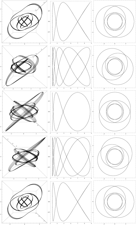
The goal here is to generalize the equatorial taxonomy to fully generic Kerr motion. We could identify fully periodic orbits and argue that all generic orbits are approximated at arbitrary precision by that set of measure zero levin2008 . However, it is sufficient to consider the less restrictive, larger set of orbits that are periodic only in , as these will be shown to be perfectly periodic when projected into an instantaneous orbital plane, as illustrated in Fig. 1.
A series of orbits is shown in on the leftmost column of Fig. 1, in the plane in the middle column, and projected in an effective orbital plane in the final column. These orbits are closed in and also in the orbital plane, but are not fully closed in . The following sections will be devoted to realizing this argument. Similar reasoning led to a taxonomy of generic orbits in a Post-Newtonian expansion of two black holes in Ref. levin2008:2 ; grossman2008 .
II The Basics
We begin with the Kerr metric in Boyer-Lindquist coordinates and geometrized units and the conventional choice of :
| (2) | ||||
where
| (3) | ||||
Carter reduced the equations to first integrals of motion carter1968 ; misner , exploiting the four constants of motion and :
| (4a) | ||||
| (4b) | ||||
| (4c) | ||||
| (4d) | ||||
We will often refer to equations (4) as the Carter equations. In those equations, an overdot denotes differentiation with respect to Mino time mino2003 , , which is related to the particle’s proper time, , by , and the quantities
| (5) | ||||
| (6) | ||||
are the polar and radial quasi-potentials, respectively wilkins1972 .
The quasi-potentials reveal some well-known geometric information about bound non-plunging orbits (orbits that neither escape to infinity nor cross the horizon of the central black hole). First, they reveal the radial turning points, which occur at roots of . For a given and , the quartic polynomial has four roots. The outermost two are periastron and apastron, between which the radial position of a bound orbit oscillates. A similar analysis of the roots of reveals that every bound orbit oscillates between a fixed and symmetrically distributed about the equatorial plane111For equatorial orbits, ., i.e. levin2008:3 ; wilkins1972 ; hughes2001 . The upshot is that every orbit will generally lie in a toroidal wedge around the equatorial plane bounded and in radial coordinate and between and in polar angle drasco2006 .
Every bound Kerr orbit also has an associated triplet of fundamental frequencies , which can be defined for any choice of time coordinate schmidt2002 . The simplicity afforded by the choice of Mino time and exploited heavily in mino2003 ; drasco2004 is that, since the radial and polar motions decouple in Mino time, each of and is independently periodic. As a result, the Mino-time frequencies can be defined and computed directly from equations (4a) and (4b).
We will only be concerned with the radial and polar frequencies here. To obtain them, we first define the radial and polar Mino periods via
| (7a) | ||||
| (7b) | ||||
The corresponding Mino-time frequencies are then
| (8a) | ||||
| (8b) | ||||
Note that we use Mino time purely for ease and convenience and that the frequency ratios which figure prominently in our analysis are independent of the choice of time variable.
We want to consider orbits that are closed in . That closure will result when the polar and radial frequencies are rationally related, or in language more directly useful for our orbital plane description of the motion, when the quantity
| (9) |
is rational. To be useful, a classification based on orbits with rational has to have two properties: the rational must tell us about the topology of the orbit, and it must relate that topology to more physical conserved quantities. In the subsequent sections, we show that this is indeed the case.
II.1 The Energy Spectrum
In the spirit of the equatorial classification of levin2008 , we begin by describing how varies with energy. For ease, and in anticipation of the fact that our analysis will ultimately focus on the discrete set of values for those orbits with rational values of , we will refer (loosely) to the dependence of on as an energy spectrum. The subtlety in establishing a simple relationship between and is the choice of which other parameters to keep fixed as is varied. In the appendix we show that the key combinations are an effective total angular momentum and angle of inclination for orbits around a black hole of a given spin defined by
| (10) | ||||
first used by ryan1995 ; ryan1996 and used occasionally in other references drasco2006 ; hughes2001 ; hughes2001:2 ; glampedakis2002:2 . Our construction turns out to be greatly facilitated by varying while keeping fixed, as opposed to varying while keeping fixed.
This choice of orbital parameters allows us to write equations (5) and (6) as
| (11) | ||||
| (12) | ||||
With this particular combination of constants, we can produce an analog of the familiar Schwarzschild effective potential for nonequatorial Kerr motion. Consider a black hole of given spin . For a non-spinning black hole (), we can rewrite the radial equation (4a) as
| (13) |
This standard effective potential formulation of Schwarzschild motion relates the radial velocity with respect to particle proper time to an effective energy and an effective potential that is a different function of for each fixed – crucially, is independent of . The result is a simple visual way to describe the different types of allowed motion as is varied.
However, for fully orbits around a spinning black hole, an analogous potential is not self-evident. The counterpart to equation (13) (which must involve velocities with respect to Mino-time in order to decouple the radial motion from the polar motion) is
| (14) |
In this case, the dependence on in cannot be simply separated and moved to the right-hand side. It would seem that the best we can do with eqn. (14) is end up with a that depends on all the constants of motion. We therefore lose the ability to visualize easily the variation of orbits with energy, as we can in the Schwarzschild case, because even at fixed and (or and ), changing also causes the potential to shift. As written, then, equation (14) admits a one-dimensional effective potential description, but that description is not useful because there is a different potential for every combination of orbital parameters.
However, if we consider only the behavior at the turning points, we can construct a useful pseudo-effective potential. The idea is to set in Eqn. (14), which amounts to setting , and to solve for :
| (15) |
. We then define a pseudo-effective potential
| (16) |
that will allow us to draw various lines of fixed on a potential that maintains its shape and visually identify turning points of the motion, even if the difference between and the value of no longer gives the value of .
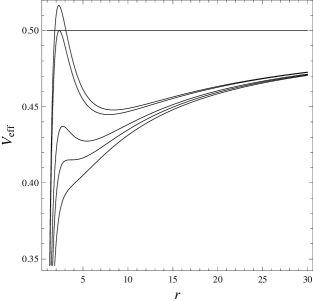
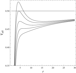
Fig. 2 illustrates the utility of this approach. For every fixed , as is lowered we get an analogous pattern of orbits to the Schwarzschild case. There is a minimum of , which corresponds to a stable constant radius orbit. There is a maximum of , which corresponds to an unstable constant radius orbit. Unlike the Schwarzschild case, the constant radius orbits are not circles. Instead they lie on the surface of a sphere bounded between and . We hereafter call these spherical orbits.
The parallel story continues. As is lowered, the unstable spherical orbit becomes bound once a certain critical value is crossed. That value is the angular momentum of the innermost bound spherical orbit (ibso), the unstable spherical orbit with critical energy . An innermost stable spherical orbit (isso) appears as a saddle point of once drops to yet another critical value . For , all orbits plunge into the central black hole. Fig. 2 demonstrates the consistency for both prograde and retrograde orbits.
If we had chosen to keep fixed while varying instead of keeping fixed while varying , we would not have seen the same simple pattern. Appendix B shows the breakdown in the Schwarzschild analogy when using orbital parameters .
The result, for a given , is that increases monotonically with energy. The lowest energy bound orbit is the stable spherical orbit, and, importantly, this orbit has the lowest value of for that combination of . As detailed in Ref. levin2008 , the constant radius orbits do not have rational value zero, as can be proven by taking the zero eccentricity limit, .
Since is monotonic, its upper bound is the value of for the maximum energy bound non-plunging orbit for a given . Whether is finite or infinite depends on whether is greater than or less than . If , the unstable spherical orbit is unbound and has energy . is therefore the value of the orbit, and despite the fact that the orbit just reaches after infinite time, its is nonetheless finite. As we reduce , increases monotonically, and eventually once . For all , remains infinite levin2008:3 ; perez-giz2008 . This happens because the maximum energy bound non-plunging orbit is now the homoclinic orbit (or separatrix orbit), which formally has an infinite number of whirls during its lone infinite-period radial cycle. A detailed analysis of the homoclinic orbit can be found in levin2008:3 ; perez-giz2008 .
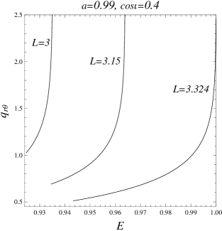
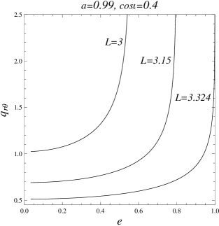
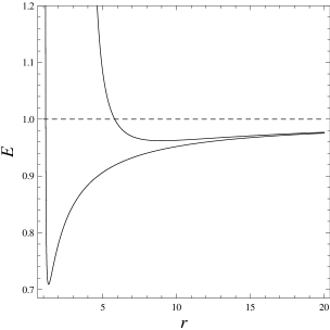
Figure 3 is a plot of the versus energy for a given and sets of values. It is representative of the general trend we see for any combination222The case of needs to be handled as in Ref. levin2008 because that is motion that takes place entirely in the equatorial plane. of . As the energy increases, so does . As decreases towards , the minium value of increases. This trend was seen equatorially in Ref. levin2008 .
In figure 3 we see that the also increases with eccentricity, . Again this is a general trend so that is monotonic with eccentricity. The larger , again for a fixed , the more eccentric the orbit.
We have shown that corresponds to an energy spectrum for orbits. What we want now is to show this also corresponds to a measure of zoom-whirliness and so is also a toplogical indicator. As we will see, quite incredibly, this measures the amount by which the angle in the orbital plane overshoots , that is, precesses, in one radial period. In other words, when is rational, it is a direct measure of the topology of the orbit in the orbital plane and increases monotonically with energy, thereby defining a spectrum of zoom-whirl orbits in the orbital plane.
II.2 Periodic Tables and the Orbital Plane


We preface this section with the caveat that the orbital plane construction below naively employs flat space vector algebra and vector calculus constructions (e.g. cross products of 3-vectors) without fully taking into account the curvature of the background Kerr spacetime. Prima facie, it is not obvious that the formalism should accurately capture geometric or topological features of 3D orbits. Nevertheless, we have the amazing result that the periodic orbits correspond to a spectrum of zoom-whirl orbits in this effective orbital plane, beautifully mirroring the equatorial result of Ref. levin2008 . For now, we simply state our results, which are compelling, and report that a more precise analysis of the connection between the orbital plane construction and a relativistically precise projection of the motion using local tetrads is underway. A very precise implementation for the PN-expansion of two black holes can be found in Refs. levin2008:2 ; grossman2008 .
We consider the projection of periodic orbits in an instantaneous orbital plane that we define naively as the plane in the tangent space spanned by and , defined below, with a corresponding angular momentum . At every instant, the orbital plane is the plane perpendicular to the angular momentum vector.
It is useful to define
| (17) |
and convert from ellipsoidal to Cartesian coordinates
| (18) |
Then,
| (19) |
where
for which
| (20) |
where and . For convenience we take the limit carroll ,
so that
| (22) |
To find the orbital plane, we write
| (23) |
so that we can define
| (24) |
The orbital plane is spanned by . (For a more detailed exposition on the orbital plane variables, see Ref. levin2008:2 ; grossman2008 .) This informally defined orbital plane is sufficient, as we will see, since it effectively soaks out any motion.
Fig. 4 shows a table of orbits in the effective orbital plane. Our periodic table assembles orbits with rational as an energy spectrum, with energy increasing from top to bottom and then from left to right. The topology of zoom-whirl orbits in the effective orbital plane is encoded in through
| (25) |
where is the number of nearly circular whirls and indicates the order in which the zooms, or leaves, are traced out. So the orbit is a -leaf clover, that executes whirls during each each radial cycle before it moves to the leaf in the pattern.
This result is quite remarkable: is a measure of the number of times the orbit returns to per radial cycle, yet it gives topological information about the degree of precession in a very different angular variable, namely the angle swept out in the oribtal plane. Had we instead projected the orbit onto the plane, our periodic orbits would look like Lissajous figures as in Fig. 5. The geometric information in Fig. 4 is severely obscured when the trajectories are plotted as Lissajous figures.
Fig. 1 shows trajectories with the same orbital parameters but different phasing. All orbits have the same and therefore the same . However, coincides with different initial values of in the range for each picture. Under shifts in phase, the orbits are all rather different (illustrated in the first column) as are their corresponding Lissajous figures (illustrated in the second column). Notice, in stark contrast, that varying the initial phasing of -vs.- merely corresponds to an overall rotation of the very same zoom-whirl orbit in the orbital plane (illustrated in the final column).
III Summary
Our results are neatly summarized in Figures 4 and 1. Fig. 4 illustrates that orbits periodic in assemble into a spectrum of multi-leaf clovers when projected in a loosely defined orbital plane. The topology of the orbit is encoded in a rational number , from which one can immediately read off the number of leaves (or zooms), the ordering of the leaves, and the number of whirls. For a given , the rational number monotonically increases with energy and with eccentricity. So, a simple -leaf clover () has less energy and is less eccentric than a -leaf () of the same . Significantly, the rational number is bounded below so that there are no orbits in the strong-field regime. There are therefore no tightly precessing elliptical orbits in the strong-field regime. All eccentric orbits will have a countable number of leaves.
Moreover, as Fig. 1 illustrates, a change in phase corresponds to a simple rotation of the orbit in the effective orbital plane. An orbit that hits apastron at will be rotated by in the orbital plane relative to an orbit with identical that hits apastron at .
Any aperiodic orbit will be arbitrarily well-approximated by a nearby periodic orbit. What’s more, aperiodic orbits will look like precessions of low-leaf clovers. Just as Mercury is a precession of the ellipse, an orbit with is the precession of a -leaf clover that accumulates an extra of azimuth during each radial cycle. Our results therefore provide a complete taxonomy for generic Kerr orbits.
**Acknowledgements**
This work was supported by an NSF grant AST-0908365. JL gratefully acknowledges support of a KITP Scholarship, under Grant no. NSF PHY05-51164.
Appendix A Spherical Orbits
In the cases of Schwarzschild and equatorial Kerr motion, orbits of constant — circular orbits — serve to organize the ranges of orbital parameters over which bound, nonplunging motion exists. Constant orbits in the general Kerr geometry play a similar organizational role but need not lie in a plane. Thus, they are not necessarily circular orbits but rather spherical. Spherical orbits were first treated in wilkins1972 and later analyzed in the context of radiation reaction in hughes2001 ; hughes2001:2 (in the latter references, these constant orbits are refered to as “circular, nonequatorial orbits”, but we use the original shorter moniker “spherical” from Ref. wilkins1972 ). Like circular orbits, spherical orbits have ; unlike their circular counterparts, spherical orbits do not have .
An initial analysis of equatorial Kerr motion (we can think of Schwarzschild motion as the subcase) begins with expressions for and of circular orbits as a function of and the (fixed) central black hole spin . Our generic Kerr analysis will reproduce one such equatorial-like picture for each inclination and will have an effective total angular momentum take the place of the more conventional conserved quantity but otherwise proceed analogously. We therefore turn now to deriving expressions for the effective angular momentum and of spherical orbits as functions of and . Ref. hughes2001 has similar expressions for and of spherical orbits in terms of and , but as we explain in Appendix B, aggregating orbits with fixed values of the constants and is most conducive to a clear exposition of the dynamics.
As in the equatorial Kerr case, our starting point is the radial quasi-potential . We begin by expressing and its derivatives in terms of and . From eqn. (12),
| (26) | ||||
| (27) | ||||
| (28) | ||||
The condition implies from equation (4a). Solving for from equation (4a) we find that
where . We can see immediately from equation (A) that implies . Similarly, implies that .
To find expressions for all and for a fixed and , we set and solve for and . Solving the two coupled quadratic equations yields four solutions for each of and . We determine the physically admissible solutions by imposing that always be positive, i.e. an effective angular momentum magnitude. Additionally, because each fixed should replicate the orbital structure of the Schwarzschild geometry, both the and solutions should asymptote at low -values to the innermost time-like spherical orbit. There should also be a minimum and value corresponding to the innermost bound spherical orbit (ibso). And the at which the minima occur on the and graphs should be the same. Finally, at large , our plot should reproduce the Newtonian limit, and should asymptote to .
Combining the above conditions, we find
| (30) | ||||
| (31) | ||||
. We recover the functions and given in bardeen1972 for equatorial Kerr circular orbits by setting for prograde and for retrograde in equations (30) and (31). From there, we recover the well-known Schwarzschild functions and (see, for instance, Ref. carroll ) by setting in (30) and (31) (note that, by spherical symmetry, those values must be and are independent of ).
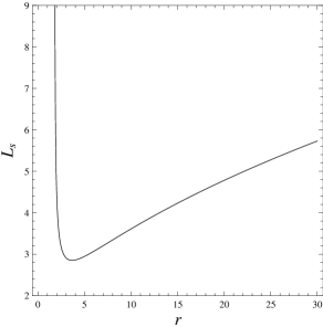
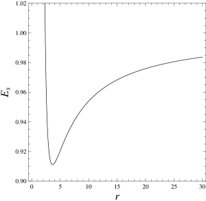
Figure 6 shows both and as functions of with parameters and . The following qualitative features are representative of all and values and mimic the features of Schwarzschild. Both and have minima that occur at the same . The minimum , , corresponds to the least for which there exists a spherical orbit. The plot corresponding to has a saddle point where the stable and unstable spherical orbits merge. For all there are two spherical orbits, whose -values exactly correspond to the local minimum and maximum of the effective potential plots of that . The maximum is the unstable spherical orbit and the minimum is the stable spherical orbit. There is a critical value at which the unstable spherical orbit has , and for all , the unstable spherical orbit is unbound with . For a fixed and , all the qualitative properties of the generic Kerr orbits replicate the Schwarzschild system.
The innermost bound spherical orbit, ibso, is defined as the spherical orbit with critical energy . To find the and , we set (26) and (27) to zero with . The innermost stable spherical orbit, isso, is the minimum of the plot and is subject to the further constraint . We therefore find the isso for a given and by setting all three of equations (26), (27) and (28) to zero simultaneously and solving for , and .
Appendix B Choosing conserved quantities
The Kerr metric has four conserved quantities. They are conventionally chosen to be the black hole mass (), the orbital energy (), the -component of angular momentum () and the carter constant (). Because each of those quantities are constants of the motion, any combination of them is also a constant of the motion. Therefore, there are an infinite number of choices of four independent quantities we could make for our conserved quantities.
We have chosen to use , , effective angular momentum (, where ) and inclination angle (, where ). This section provides an explanation for our choice.
Our goal was to realize a generic Kerr orbit structure that generalized the Schwarzschild and equatorial Kerr orbit structures presented in levin2008 . To bring that goal to fruition, we look for a set of conserved quantities such that we could hold one fixed and reproduce all the qualitative features of Schwarzschild dynamics (isso, ibso, etc.).
Using the conventional , and , the equatorial Kerr system is defined by . There are two sets of and solutions for circular orbits, one prograde and one retrograde. Figure 7 shows the two solutions for and . We can see that the solutions never intersect and each solution has all the qualitative features present in the standard organization of Schwarzschild orbits.
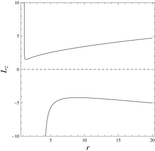
However, when becomes large enough, regardless of the spin, we see a loss of adherence to these features. Specifically, there is no longer an isso, and the two sets of solutions for and for a fixed mix. While this phenomenon is not seen until gets large, it is present for all spin values. The discontinuity in the and spherical graphs, as well as the loss of the isso is seen for the full range of values.
The upshot is that there are values of that do not allow us to reproduce the familiar qualitative organization of Schwarzschild dynamics if we choose to look at orbits of constant as an ensemble. In contrast, we find that with , for every fixed , the qualitative dynamical picture mimics the familiar Schwarzschild one beautifully. In this picture, each corresponds to a fixed orbital inclination so that equatorial orbits correspond to one of two values: for prograde, and for retrograde. Furthermore, whereas each fixed admits two associated and solutions each for spherical orbits, each produces only one curve each for and .
Figure 8 shows a set of and plots for spherical orbits with . We can see the loss of the isso and the mixing of the two seperate solutions. The curves are no longer even single-valued at a given . Moreover, the curve can have more than 2 orbits with a given , as opposed to only the stable and unstable constant orbits we are used to in the Schwarzschild effective potential picture. We have picked four points on the fixed plots, each with a unique set of orbital parameters, , and . For each of those points, we have determined the corresponding , and and plotted the and curves for each of those values. Notice that there is no such breakdown when we look at curves of fixed rather than fixed . Instead, the latter curves faithfully reproduce the expected qualitative features of the corresponding Schwarzschild or equatorial Kerr curves.

References
- (1) B. Carter, Phys. Rev. 174, 1559 (1968).
- (2) C. W. Misner, K. S. Thorne, and J. A. Wheeler, Gravitation, W. H. Freeman, first edition, 1973.
- (3) J. Levin and G. Perez-Giz, Phys. Rev. D 77, 103005 (2008).
- (4) J. Levin, Class. Quant. Grav. 26, 235010 (2009).
- (5) J. Levin and R. Grossman, gr-qc/08093838 (2008).
- (6) R. Grossman and J. Levin, gr-qc/08113798 .
- (7) Y. Mino, Phys. Rev. D67, 084027 (2003).
- (8) D. C. Wilkins, Phys. Rev. D5, 814 (1972).
- (9) J. Levin and G. Perez-Giz, Homoclinic Orbits around Spinning Black Holes I: Exact Solution for the Kerr Separatrix, 2008.
- (10) S. A. Hughes, erratum-ibbid.d 63, 049902 (2001).
- (11) S. Drasco and S. Hughes, Phys. Rev. D 73, 024027 (2006).
- (12) W. Schmidt, Class. Quant. Grav. 19, 2743 (2002).
- (13) S. Drasco and S. A. Hughes, Phys. Rev. D 69, 044015 (2004).
- (14) F. D. Ryan, Phys. Rev. D52, 3159 (1995).
- (15) F. D. Ryan, Phys. Rev. D53, 3064 (1996).
- (16) S. A. Hughes, Phys. Rev. D 64, 064004 (2001).
- (17) K. Glampedakis, S. A. Hughes, and D. Kennefick, Phys. Rev. D 66, 064005 (2002).
- (18) G. Perez-Giz and J. Levin, Homoclinic Orbits around Spinning Black Holes II: The Phase Space Portrait, 2008.
- (19) S. Carroll, Spacetime and Geometry: An Introduction to General Relativity, Benjamin Cummings, 2003.
- (20) J. M. Bardeen, W. H. Press, and S. A. Teukolsky, Ap. J. 178, 347 (1972).