Visit: ]http://www.cond-mat.physik.uni-mainz.de/ weigel
Connected component identification and cluster update on GPU
Abstract
Cluster identification tasks occur in a multitude of contexts in physics and engineering such as, for instance, cluster algorithms for simulating spin models, percolation simulations, segmentation problems in image processing, or network analysis. While it has been shown that graphics processing units (GPUs) can result in speedups of two to three orders of magnitude as compared to serial codes on CPUs for the case of local and thus naturally parallelized problems such as single-spin flip update simulations of spin models, the situation is considerably more complicated for the non-local problem of cluster or connected component identification. I discuss the suitability of different approaches of parallelization of cluster labeling and cluster update algorithms for calculations on GPU and compare to the performance of serial implementations.
pacs:
05.10.Ln, 75.10.Hk, 05.10.-aI Introduction
Due to their manifold applications in statistical and condensed matter physics ranging from the description of magnetic systems over models for the gas-liquid transition to biological problems, classical spin models have been very widely studied in the past decades. Since exact solutions are only available for a few exceptional cases baxter:book , with the steady increase in available computer power and the advancement of simulational techniques, in many cases computer simulations have become the tool of choice even above the more traditional variational and perturbative techniques binder:book2 . The workhorse of Monte Carlo simulations in the form of the Metropolis algorithm metropolis:53a is extremely general and robust, but suffers from problems of slowed down dynamics in the vicinity of phase transitions, or for systems with complex free-energy landscapes. For the case of continuous phase transitions, critical slowing down is observed with autocorrelation times increasing as with in the vicinity of the critical point. This divergence of temporal correlations is a consequence of the divergent critical correlations in space, compared to which local modifications of the configuration become inefficient. An exceptionally successful solution of this problem is given by a class of cluster-update algorithms working on stochastically defined connected regions of spins with identical or similar orientation swendsen-wang:87a ; wolff:89a ; kandel:91a ; kawashima:95a , which allow for a significant reduction of the dynamical critical exponent over the local value and can thus easily lead to an effective speed gain in excess of for practically considered system sizes. Incidentally, the practical task of cluster identification resulting from the probabilistic description of the problem as a bond-correlated percolation model is identical to that encountered in image segmentation or computer vision, where neighboring pixels should be lumped together according to their colors, a problem which can be mapped to the Potts model opara:98 ; wang:08 . Also, numerical simulations of percolation problems, with their wide range of realizations from fluids in porous media to epidemic spreading stauffer:book , must deal with a very similar problem of cluster identification (see, e.g., Ref. hoshen:79 ). Further applications occur in network analysis, particle tracking or the identification of structures such as droplets in condensed matter. Efficient implementations of cluster labeling algorithms are, therefore, of significant interest for a number of different applications in scientific computing.
In parallel to the invention of new simulation algorithms, the need for strong computing power for tackling hard problems has prompted scientists to always make the best use of the available computer resources of the time, be it regular PCs, vector computers or Beowulf clusters. For the case of simulations of spin models, for instance, a number of special purpose computers has been devised, including machines for local updates such as JANUS for spin glasses belleti:09 and variants such as the “cluster processor” using cluster-update algorithms bloete:99a . While these were (and are) highly successful in their specific application fields, their design and realization is a rather challenging endeavor, costly in terms of monetary as well as human resources. It is therefore desirable to search for a less application specific, but still highly performant platform for massively parallel scientific computing that is less expensive in terms of its acquisition as well as its power consumption and cooling requirements than traditional cluster computers. An architecture meeting those standards has become available in recent years with the advent of general purpose computing on graphics processing units (GPUs) owens:08 ; kirk:10 . With the availability of convenient application programming interfaces (APIs) for GPU computing, most notably NVIDIA CUDA and OpenCL kirk:10 , the programming effort does no longer dramatically exceed that of CPU based parallel machines. Still, for efficient implementations architectural peculiarities of these devices, in particular the organization of compute units (cores) in groups (multiprocessors) with reduced synchronization capabilities between multiprocessors and the pyramid of memories with latencies, sizes and access scopes decreasing from base to tip, need to be taken into account. For the case of spin models, a wide range of simulation algorithms with local updates has been previously implemented on GPU preis:09 ; bernaschi:10 ; weigel:10a ; ferrero:11 , where for the implementations reported in Refs. weigel:10c ; weigel:10a ; weigel:11 significant speedups of two to three orders of magnitude as compared to serial CPU codes have been reported. An efficient parallelization of non-local algorithms and cluster labeling is significantly more challenging, however, in particular for the case of cluster updates for spin models close to criticality, where the relevant clusters undergo a percolation transition and are therefore spanning the whole system heermann:90 ; baillie:91 ; mino:91 ; apostolakis:92 ; barkema:94 ; bauernfeind:94 ; flanigan:95 ; martin-herrero:04 .
The implementations discussed here have been realized within the NVIDIA CUDA cuda framework with benchmarks performed on the GTX 480, GTX 580 and Tesla M2070 GPUs. While some of the details are specific to this setup, the algorithmic approaches discussed are fairly general and could easily applied to other GPU devices or realized with different APIs such as OpenCL. For an introduction into the details of the GPU hardware and the corresponding programming models, the reader is referred to the available textbooks (see, e.g, Ref. kirk:10 ) and previous articles by the present author weigel:10c ; weigel:10a .
The rest of the paper is organized as follows. In Section II GPU implementations of the cluster algorithm of Swendsen and Wang swendsen-wang:87a are discussed. The cluster decomposition of the complete spin lattice necessary here is identical to that of a corresponding image segmentation problem or percolation simulation. Section III is devoted to the case of the single-cluster variant suggested by Wolff wolff:89a . Finally, Section IV contains my conclusions.
II Swendsen-Wang algorithm
In this paper, I focus on the ferromagnetic -state Potts model with Hamiltonian
| (1) |
where denote the spin variables, is the exchange coupling, and the sum extends over all bonds of an underlying graph, most commonly a regular lattice. In dimensions , the model undergoes a transition from a disordered phase at high temperatures to an ordered phase where one of the states prevails at low temperatures wu:82a . For , the transition is continuous for and first order for , while in it is first order for any . The special case is equivalent to the celebrated Ising model. A local Monte Carlo simulation of the Potts model proceeds by iteratively changing the orientation of randomly chosen spin variables in accordance with the detailed balance condition binder:book2 . In contrast, the cluster algorithm of Swendsen and Wang swendsen-wang:87a updates connected components of (usually) more than one spin and is based on the following transformation of the partition function due to Fortuin and Kasteleyn fortuin:72a ,
| (2) | |||||
| (3) | |||||
| (4) |
where denotes the inverse temperature and . In Eq. (4), a set of auxiliary bond variables is introduced, where whenever and with probability for . The resulting stochastically defined clusters are therefore subsets of the geometric clusters of parallel spins. Using a graphical expansion of the term in square brackets in Eq. (4) and summing over the spin configurations , it can be shown that the model is equivalent to a generalized percolation model with partition function fortuin:72a ; hu:84a
| (5) |
known as the random-cluster model. Here, denotes the number of activated edges resulting from the bond variables , is the number of connected components of the induced subgraph, and is the total number of edges in the underlying graph or lattice. From the percolation representation (5) it is clear coniglio:80a that the stochastic clusters induced by the bond variables (and not the geometric clusters of like spins) undergo a percolation transition at the thermal transition point, and hence it is these structures that should be updated to efficiently decorrelate the system close to criticality.
Utilizing the representation (4) the algorithm by Swendsen and Wang alternatingly updates spins and bond variables as follows:
-
1.
For a given spin configuration set for each bond with . Set and with probabilities and , respectively, for each bond with .
-
2.
Identify the connected components of the subgraph of the lattice induced by the bond variables .
-
3.
Choose a new spin orientation randomly in for each connected component and update the spin variables accordingly.
Since clusters of single spins are possible, this update is trivially ergodic. It is straightforward to show that detailed balance is fulfilled swendsen-wang:87a ; kawashima:95a . Hence, the Swendsen-Wang (SW) dynamics forms a valid Markov chain Monte Carlo algorithm of the Potts model. Autocorrelations are dramatically reduced as compared to local spin flips. A rigorous bound for the dynamical critical exponent is li:89 , where is the exponent of the scaling of the integrated autocorrelation time and and are the (static) critical exponents of the specific heat and the correlation length, respectively. This bound is close to sharp in two dimensions deng:07a , but not in where, nevertheless, significant reductions in autocorrelations and the dynamical critical exponent are observed.
Attempting a highly parallel GPU implementation of the SW algorithm, it is clear that the bond activation in step 1 as well as the cluster flipping in step 3 can be rather easily parallelized as they are perfectly local operations. In contrast, the cluster identification in step 3 must deal with structures spanning the whole system, in particular for simulations close to criticality which are the main strength of cluster updates. This is also the crucial step for further applications of cluster identification such as the image segmentation problem mentioned above. The total run time for a single update of the spin lattice with the SW algorithm on a single GPU therefore decomposes as
| (6) |
We distinguish these times from the corresponding serial run times , , etc. for single-threaded calculations. For definiteness, the implementation is discussed in some detail for the specific example of the Potts model on the square lattice of edge length with periodic boundary conditions. Generalizations to three dimensions or other lattice types are straightforward.
II.1 Bond activation
We use an array of char variables to represent the bond activation states . For the GPU implementation using CUDA kirk:10 , bond activation is performed by a first kernel, prepare_bonds(). Given a configuration of the spins , for each bond an expression of the form
| (7) |
needs to be evaluated, where is a uniform (pseudo) random number, and . To enable parallelism, the system is broken up into tiles of spins, and each tile is assigned to an independent thread block. If we denote , and the number of tiles, the expected parallel run time behaves as
| (8) |
where denotes the number of multiprocessors ( for Tesla M2070, for GTX 480, for GTX 580), is the number of cores per multiprocessor ( for all three cards), and is the number of sites assigned to each thread111I do not take the effects of latency hiding and other scheduling specificities into account in the scaling formulae, but discuss them in some places in connection with observed deviations from these simplified laws. It is also assumed that the number of threads per block is at least since due to the limitation to eight active blocks per multiprocessor on current NVIDIA GPUs, there would otherwise be idle cores.. For large systems, and , Eq. (8) reduces to . As discussed in detail in Refs. weigel:10c ; weigel:10a , each thread requires its own instance of a random number generator (RNG) to prevent the formation of a performance bottleneck. Due to the resulting large number of RNG instances (for the case of large systems), one requires a generator with a small state comprising, ideally, not more than a few bytes. This precludes the use of high-quality, but large state generators such as Mersenne twister matsumoto:98 in applications of the type considered here. Additionally, one needs to ensure that the thus created streams of random numbers are sufficiently uncorrelated with each other. Suitable generator types for this purpose are, for instance, arrays of linear congruential generators with random seeds, which are fast but might not produce random numbers of sufficient quality gentle:03 ; preis:09 ; weigel:10a , generalized lagged Fibonacci generators weigel:10a , or the Marsaglia generator as suggested in Ref. ferrero:11 . As the cluster identification step, which does not require random numbers, dominates the parallel runtime of the algorithm, RNG speed is not as important as in local update simulations on GPUs. For the benchmarks reported below, I used an array of 32-bit linear congruential generators. Statistically significant deviations from the exact results ferdinand:69a for the Potts model at criticality have not been observed.
An analysis of the kernel with CUDA’s Compute Visual Profiler cuda shows that its performance is compute bound. Still, memory performance can be improved by using an appropriate memory layout ensuring that reads of subsequent threads in the spin and bond arrays map to consecutive locations in global memory to ensure coalescence of memory requests kirk:10 . With a linear memory arrangement these requirements are best met when using tiles with . Best results for systems with are found here for , (considering only lattice sizes , ). Evaluating the acceptance criterion leads to unavoidable thread divergence, but the effects are not very dramatic here. The asymptotic performance of the kernel with one spin per thread, , is ns on the GTX 480 (assuming full loading of the multiprocessors which is reached for sufficiently large systems). An alleviating effect on thread divergence and memory limitations is reached by assigning several spin pairs (bonds) to each thread. Two versions have been considered here, either assigning a (square) sub-block of four spins to each thread (), which brings down the updating time to ns, or assigning only threads per tile, each of which has to update spins, leading to the same asymptotic performance of ns on the GTX 480. The better performance of these variant kernels has to do with the possibility of pre-fetching of data into registers while arithmetic operations are being performed. The same kernel is used to also initialize the cluster labels (see below). Note that the relatively lower performance of this kernel as compared to the Metropolis update of the Ising model reported in Ref. weigel:10a of about ns per spin (without multi-hit updates) on the same hardware is explained by the 6-fold increase in memory writes (two chars and one int versus one char) and the use of two random numbers (instead of one) per spin.
II.2 Cluster labeling on tiles
To allow for an efficient use of parallel hardware, cluster labeling is first performed on (square) tiles of spins and cluster labels are consolidated over the whole lattice in a second step (see Sec. II.3 below) heermann:90 ; baillie:91 ; mino:91 ; barkema:94 ; bauernfeind:94 ; flanigan:95 . Hence the time for cluster identification naturally breaks up into two contributions,
| (9) |
In the field of simulations of spin systems (and percolation), the standard technique for cluster identification is due to Hoshen and Kopelman hoshen:79 . Although originally not formulated in this context, it turns out to be a special version of the class of union-and-find algorithms well known in theoretical computer science cormen:09 . Time and storage requirements for this approach scale linearly with the number of sites. A somewhat more “natural” approach consists of a set of breadth-first searches on the graph of bonds, growing the clusters in a layered fashion. While storage requirements are super-linear in (and might be as large as depending on the structure of the underlying graph), computing time scales still linear in and implementations are typically very straightforward and efficient. A third approach considered here, dubbed self-labeling baillie:91 , is very inefficient regarding (serial) computing time, but very well suited for parallelization.
II.2.1 Breadth-first search
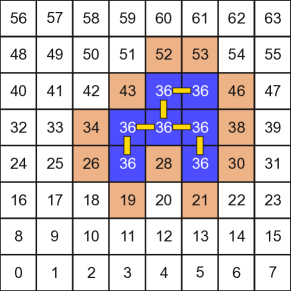
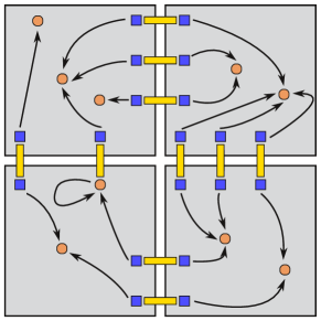
In breadth-first search (or “ants in the labyrinth”) the unvisited neighbors of a starting vertex or seed that are connected by activated bonds are examined and stored in a first-in-first-out (FIFO) data structure (a queue). Subsequently, nodes are removed from the queue in the order they have been stored and examined in the same fashion as the initial vertex. This leads to a layered growth of the identified part of a cluster as illustrated in Fig. 1. The complete set of clusters is being identified by seeding a new cluster at each node of the lattice that is not yet part of a previously identified cluster. Information about the cluster structure is stored in an array of cluster labels, where originally each cluster label is initialized with the site number on the lattice and cluster labels are set to that of the seed site on growing the cluster, cf. Fig. 1. While this approach is very general (it can be applied without changes to any graph) and well suited for serial calculations, it is not very suitable for parallelization bader:06 . Parallelism can be implemented in the examination of different neighbors of a site and in processing the sites on the wave front of the growing cluster. To avoid race conditions and achieve consistency of the data structures, however, locks or atomic operations are required, considerably complicating the code. Additionally, the number of (quasi) independent tasks is highly variable as the length of the wave fronts is fluctuating quite strongly. For the case of a parallel identification of all clusters as necessary for the SW algorithm and image segmentation, this approach is hence not very well suited for a GPU implementation. A parallel implementation will be discussed below in the context of the single-cluster (or Wolff) variant of the algorithm in Sec. III, however.
The parallel run time of this kernel, local_BFS(), employing one thread per block performing cluster identification in a tile of edge length , is therefore expected to scale as
| (10) |
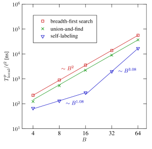
The measured run times for follow this expectation, resulting in perfectly linear scaling of the time per tile with the number of tile sites, cf. Fig. 2. Since only a maximum of 8 thread blocks can be simultaneously active on each multiprocessor on current generation NVIDIA GPUs kirk:10 , however, 24 of the 32 cores of each multiprocessor are idling, leading to rather low performance. The asymptotic maximum performance for large system sizes (leading to an optimum effect of latency hiding through the scheduler) on the GTX 480 is at around ns for this kernel, local_BFS().
II.2.2 Union-and-find algorithms
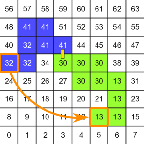
It is a well known problem in computer science to partition a set of elements into disjoint subsets according to some connectedness or identity criterion. A number of efficient algorithm for this so-called union-and-find problem have been developed cormen:09 . Consider a set of elements denoted as vertices in a graph which, initially, has no edges. Now, a number of edges is sequentially inserted into the graph and the task is to successively update a data structure that contains information about the connected components resulting from the edge insertion. Obviously, our cluster identification task is a special case of this problem. In a straightforward implementation one maintains a forest of spanning trees where each node carries a pointer to its parent in the tree, unless it is the tree root which points to itself. On insertion of an edge one determines the roots of the two adjacent vertices by successively walking up the respective tree structures (find). If the two roots found are the same, the inserted edge was internal and no further action is required. If two different roots were found, the edge was external and one of the trees is attached to the root of the other as a new branch (union), thus amalgamating two previously disjoint subsets or connected components of the graph. The forest structure can be realized with an array of node labels, where each node is initialized to point to itself (i.e., it is its own root). This process is illustrated for the present application in Fig. 3.
(Worst case) time complexity is trivially constant or for union steps, while find steps can be extensive, , if edges connecting macroscopic clusters are considered. (Storage requirements are clearly just linear in .) The complexity of the find step can be reduced by two tricks, tree balancing and path compression. Balancing can be achieved by making sure that always the smaller tree (in terms of the number of nodes) is attached to the larger. To this end, the current number of nodes is stored in the tree root. Balancing reduces the time to find the root to steps cormen:09 . Similarly path compression, which redirects the “up” pointer of each node to point directly to the tree root in a backtracking operation after each completed find task, reduces find complexity to . The combination of both techniques can be shown to result in an essentially constant find complexity for all practically relevant system sizes tarjan:75 . An implementation of the full algorithm geared towards cluster identification is described in Ref. newman:01a .
Like the breadth-first search, the tree-based union-and-find approach is intrinsically serial as all operations work on the same forest structure, whose consistency could not be easily maintained under parallel operations. Moderate parallelsim is possible in the union step, where the two find operations for the vertices connected by the new edge can be performed in parallel. Due to the resultant thread divergence, however, using two threads per block is found to actually decrease performance. Similarly, the extra effect of path compression (keeping the stack for backtracking in fast shared memory) is found to actually increase run times, at least in the range of tile sizes considered. The parallel scaling of the algorithm is thus the same (up to logarithmic corrections) as that of breadth-first search given in Eq. (10). In fact, is found to be almost perfectly linear in in the considered regime, cf. the data presented in Fig. 2. The asymptotic performance (neglecting logarithmic terms due to the find step) of the kernel local_unionfind() on the GTX 480 is found to be ns, somewhat better than for local_BFS(). Note that for the tree-based algorithms of the union-and-find type, memory accesses are inherently non-local leading to a certain performance penalty which hardly can be avoided.
II.2.3 Self-labeling
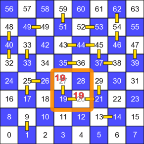
While breadth-first search and tree-based union-and-find are elegant and very efficient for serial implementations, they appear not very suitable for parallelization, especially on GPUs where groups of threads are executed in perfect synchrony or lockstep and extensive thread divergence is expensive. An antipodal type of algorithm is given by the simple approach of self-labeling baillie:91 : Cluster labels are initialized with the site numbers. Each site then compares its label to that of its eastward neighbor and sets its own and this neighbor’s labels to the minimum of the two, provided that an activated bond connects the two sites. The same is subsequently done with respect to the northward neighbor, cf. Fig. 4. (On a simple cubic lattice, the analog procedure would involve three out of six neighbors.) Clearly, the outcome of a whole sweep of re-labeling events will depend on the order of operations and several passes through the tile will be necessary until the final cluster labels have propagated through the whole system. Eventually, however, no label will have changed in a whole pass through the tile and the procedure can be stopped, leading to a correct labeling of clusters inside of each tile. Let us first concentrate on the spin model at criticality. Then, clusters typically span the tile, such that at least of the order of sweeps will be required to pass information about correct cluster labels from one end of the tile to the other. In fact, even more passes are necessary, as information about cluster labels needs to be diffusively transmitted between each pair of sites in the same cluster. Since under the chosen dynamics this information will be transmitted along the shortest path connecting the two sites, the required number of sweeps will scale as
| (11) |
where is the fractal dimension of the shortest path on a percolation cluster. For pure percolation (corresponding to the limit of the Potts model) it is found to be in and in herrmann:88 , whereas for the (Fortuin-Kasteleyn clusters of the) and Potts models in two dimensions it has been estimated as and , respectively miranda:91 . Obviously, the approach can be easily parallelized inside of tiles, assigning an individual thread to one or spins. As a consequence, the parallel run time for the self-labeling approach is
| (12) |
at or close to the percolation transition, which asymptotically appears to be rather unflattering as compared to the breadth-first search and union-and-find techniques. Due to the parallelization on the tile level, however, the total run time can still be quite low for intermediate tile sizes. Off criticality, the scaling becomes somewhat more favorable. Below the transition, where clusters span the lattice, but they are no longer fractal, should be replaced by one. Above the transition, on the other hand, with a finite correlation length , in Eq. (12) is replaced by . While this somewhat better behavior is probably not very relevant for the spin models as simulations close to criticality are the main purpose of cluster-update algorithms, it is of importance for percolation simulations or image segmentation problems for the (typical) case of a finite characteristic length scale .
Figure 2 shows the scaling of parallel run times for the kernel local_selflabel() on tiles of sizes for the Potts model at the critical point . One can clearly distinguish two regimes with scaling for and for . (The data in Fig. 2 are for on the GTX 480 with , such that the crossover occurs at .) As is apparent from Fig. 2, for tile sizes self-labeling is clearly superior in parallel performance on GPU as compared to breadth-first search or union-and-find, although it becomes less efficient than the latter two approaches for . I tested different variants: (a) an implementation, local_selflabel_small(), that assigns one spin per thread, restricting the tile size to on current NVIDIA GPUs with a limitation of 1024 threads per block, (b) a kernel local_selflabel() which assigns a block of spins to each thread, allowing tile sizes up to , and (c) a looped version, local_selflabel_block(), that assigns one column of height to each thread, such that the lines are worked on through a loop. In all cases, the relevant portion of the bond activation variables and cluster labels are copied to shared memory, such that memory fetches in the re-labeling steps are (almost) instantaneous. Bank conflicts are avoided through an appropriate layout of the data in shared memory. Depending on the number of spins per thread, a different order of operations can lead to different results for each single self-labeling pass. Consistency could be enforced via atomic operations, but these slow down the code and are found to be not necessary here. Therefore, while the number of necessary self-labeling passes might vary from run to run (or device to device) depending on scheduling specificities, the final result is deterministic and does not depend on the order of operations. The decision about the end of self-labeling is taken using the warp vote function __syncthreads_or() cuda which evaluates to true as long as any of the threads has seen a re-labeling event in the last pass. Performance differences between the mentioned three kernels are found to be relatively small. The best asymptotic performance is observed for the kernel local_selflabel() with spins per thread, as this setup avoids read/write conflicts in shared memory. For tiles of size on the GTX 480 the run time per spin is ns for all labeling passes. While the total number of operations is larger for self-labeling than for breadth-first search or union-and-find, the former is 13 and 8 times faster than the latter at , respectively, due to the easily exploited inherent parallelism.
II.3 Tile consolidation
Each of the three cluster labeling algorithms on tiles discussed above results in correct cluster labels inside of tiles, however, ignoring the information of any active bonds crossing tile boundaries. To reach unified labels for clusters spanning several tiles, an additional consolidation phase is necessary. Two alternatives, an iterative relaxation procedure and a hierarchical sewing scheme have been considered to this end.
II.3.1 Label relaxation
Cluster labels can be consolidated across tile boundaries using a relaxation procedure similar to the self-labeling employed above inside of tiles flanigan:95 . In a preparation step, for each edge crossing a tile boundary the indices of the cluster roots of the two sites connected by the boundary-crossing bond are stored in an array, cf. Fig. 5 (kernel prepare_relax()). In the relaxation phase each tile sets the root labels of its own active boundary sites to the minimum of its own current label and that of the corresponding neighboring tile. Relaxation steps are repeated until local cluster labels do not change any further. Similar to self-labeling, the number of relaxation steps scales as the shortest path between two points on the largest cluster(s), however, the relevant length scale for the relaxation procedure is now , leading to the following scaling behavior at the percolation threshold
| (13) |
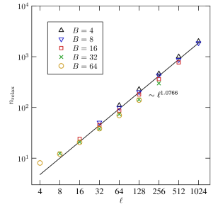
For systems below the transition temperature or more general cluster identification tasks with extensive, but non-fractal clusters, is replaced by 1, whereas above the critical point and for other problems with finite characteristic length scales . The number of iterations is shown for a simulation of the Potts model at criticality in Fig. 6. The expected scaling with miranda:91 is well observed for sufficiently large system sizes across all tile sizes : a fit of the functional form (13) results in . The small, but visible downward shift of with increasing results from concurrency effects: for a small total number of tiles many of them are treated at the same time on different multiprocessors, resulting in the possibility of a label propagating to tiles more than one step away in one pass if (as is likely) several of the boundary sites belong to the same clusters.
The number of operations per relaxation iteration is proportional to the length of the tile boundary times the number of tiles, i.e.,
| (14) |
The relaxation routine (kernel relax()) appears intrinsically serial in nature as different boundary spins can point to the same roots such that concurrent operations could lead to inconsistencies, unless appropriate locks are used. Nevertheless, an alternative implementation (kernel relax_multithread()) using threads to update a number of boundary spin pairs concurrently in a thread block is perfectly valid as similar to the self-labeling approach only the number of necessary iterations is affected by the order of operations while the final result is not changed. As different blocks can essentially only be synchronized between kernel calls, the stopping criterion is checked on CPU in between kernel invocations. The parallel run time for this kernel is then given by
| (15) |
Note that the asymptotic effort per spin from the relaxation phase, , does not become constant as the system size is increased, unless the tile size is scaled proportionally to .
For root finding in the spin-flipping phase, it is of some relevance that the relaxation process effectively attaches all sub-clusters in tiles belonging to the same global cluster directly to the root of the sub-cluster with the smallest cluster label. Therefore, the algorithm involves path compression on the level of the coarse grained lattice.
II.3.2 Hierarchical sewing
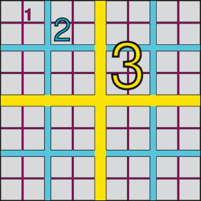
An alternative technique of label consolidation across tiles uses a hierarchical or divide-and-conquer approach as schematically depicted in Fig. 7 baillie:91 . On the first level tiles of spins are sewn together by inserting the missing bonds crossing tile boundaries. This results in larger tiles which are then combined in a second step etc. until, finally, labels of the whole system have been consolidated. For the case of periodic boundary conditions, the bonds wrapping around the lattice in both directions need to be inserted in an additional step. Bond insertion itself is performed in the union-and-find manner described above using tree balancing, i.e., the roots of the two clusters connected by the added bond are identified and the smaller cluster is then attached to the root of the larger cluster. We can assume that find times are essentially constant inside of the original tiles of size , either because tile labeling was performed with the breadth-first or self-labeling algorithms which produce labelings with complete path compression (i.e., each node label points directly to the root), or since it was done using union-and-find with (at least) one of the ingredients of tree balancing or path compression, leading to (at most) logarithmic time complexity of finds. Then, using tree balancing in the hierarchical sewing step ensures that find times remain logarithmically small as tiles are combined. Time complexity could be further improved by adding path compression, but (as for union-and-find inside of tiles) it is found here that this rather slows down the code in the range of lattice sizes considered here. Note that the self-labeling approach does not naturally provide the information about cluster sizes in the tree roots. It is found, however, that it has no adverse effect on the performance of the tile consolidation step if cluster sizes are simply assumed to be identical (and, for simplicity, equal to one) for partial clusters inside of tiles.
One thread block is assigned to a configuration of tiles at each level. The sewing itself is essentially serial in nature. For one of the two linear seams of each sewing step (the horizontal seam, say), one can use two threads, however, leading to two tiles after finishing the horizontal seam which are only combined into one larger tile by closing the vertical seam222Note that this still leads to some under-utilization of the device due to the limit of eight active blocks per multiprocessor which requires at least four threads per block for full occupancy with blocks.. As the tile size for the th generation is and the length of the seam is , the serial computational effort for level of the sewing is
| (16) |
where I have neglected logarithmic terms due to the find operations. The total number of levels is (assuming, for simplicity, that and are powers of two). Hence, the total serial effort is
| (17) |
On the GPU device with multiprocessors mapped to independent blocks available for the sewing procedure, the parallel run time for generation is
| (18) |
For a sufficiently large system, at the beginning of the process the number of tiles to sew will always exceed . As the number of remaining tiles is reduced, the number of sewing jobs will drop to reach the number of multiprocessors at or
| (19) |
where another approximation is made by allowing for non-integer level numbers . Due to the variable number of multiprocessors actually involved in the calculation, the total parallel effort has two contributions,
| (20) | |||||
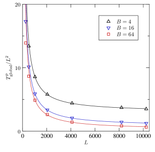
Therefore, the effort per site becomes asymptotically independent of , but this limit is approached rather slowly with a correction, whereas effects of incomplete loading of the device decay as (in two dimensions). This is illustrated by the numerical results shown in Fig. 8. The data are well described by the form
| (21) |
expected from Eq. (20). Comparing Eqs. (20) and (21), from the ratio of fit parameters one can deduce the effective number of processing units as
| (22) |
and, for instance, the fit at constant yields , while a fit at constant results in , rather close to the theoretically expected result for the GTX 480 with 8 blocks for each of the 15 multiprocessors, resulting in processing elements. The somewhat smaller estimated are attributed to effects of thread divergence and the neglect of logarithmic terms in the find step. For tile size , the asymptotic performance of this kernel if found to be ns.
II.4 Cluster flipping

Having globally identified the connected components resulting from the bond configuration, step 3 of the SW algorithm described at the beginning of Sec. II consists of assigning new, random spin orientations to each cluster and adapting the orientation of each spin in the cluster to the new orientation prescribed. Since it is inconvenient to keep a separate list of global cluster roots, it is easiest to generate a new random spin orientation for each lattice site while only using this information at the cluster roots. To this end, the array of now superfluous bond activation variables is re-used. In a first kernel, prepare_flip(), a random orientation is drawn and stored in the bond array for each site. This is done in tiles of sites as for the bond activation, using the same array of random-number generators. In a second step (kernel flip()), each site performs a find operation to identify its root and applies the new spin orientation found there to the local spin. Since cluster labels are effectively stored in a tree structure, this step involves non-local memory accesses for each site. In principle, locality could be improved here by employing full path compression in the union steps before, but in practice this is not found to improve performance for the system sizes up to considered here. Another possible improvement would eliminate the wasteful operation of drawing new proposed orientations for all spins while only the new orientations of the cluster roots are required. This can be achieved by carrying the flipping information piggy-back on the cluster labels, at least for the or Ising model where flipping information is only one bit wide. Again, however, in practice it is found that due to the incurred complications in the arithmetics regarding cluster labels in find and union operations, overall performance is actually decreased by this “optimization”. Due to the necessary tree traversal, the performance of the cluster flipping procedure depends weakly on the degree of path compression performed previously in cluster labeling on tiles and label consolidation as well as on the tile size . For the combination of self-labeling on tiles and hierarchical sewing, it is found to be ns for and , while it is somewhat smaller at ns if label relaxation is used instead of hierarchical sewing.
II.5 Performance and benchmarks
As a number of options for the cluster identification task have been discussed, the question arises which of them is the most efficient for a given set of parameters and a given GPU device. For the bond activation and cluster flipping steps, the situation is simpler as no important variants haven been discussed there, such that these steps are always performed with the outlined local approaches and tiles with and , apart from the smallest systems with . Regarding the cluster labeling in tiles, it is clear from the data presented in Fig. 2 that self-labeling shows the best performance for block sizes . The main decision is thus between the label relaxation and hierarchical sewing approaches for label consolidation. Additionally, an optimal tile size needs to be determined. For the combination of self-labeling and hierarchical sewing, the total parallel run time for cluster identification is
| (23) |
assuming that in Eq. (12). Here, and are the parameters from Eq. (21). On minimizing, the optimal tile size is then found to be
| (24) |
The fit parameters for the runs on the GTX 480 and then yield . Since, for simplicity, runs were restricted to and being powers of two, is closest to the optimum. Similar fits for the data on the GTX 580 and the Tesla M2070 also used for test runs yield the same optimum in the power-of-two step sizes. The pre-asymptotic branch with in Eq. (12) does not yield an optimum, but total run times are monotonously decreasing with . In other words, as long as idle cores in the multiprocessors are available, the tile size should be increased. hence is also the global optimum for this setup.
For the combination of self-labeling and label relaxation, the total run time for an update is
| (25) |
such that the optimal tile size becomes
| (26) |
which (with ) is approximately proportional to for the critical Potts model in two dimensions. Figure 9 shows the resulting optimal tile size as a function of . Due to the limitation of shared memory to kB on current NVIDIA GPUs, self-labeling on tiles is limited to block sizes (assuming , , , ), such that the optimal tile sizes cannot be used for . Working directly in global memory is no option as it slows down the code dramatically. Using breadth-first search or union-and-find on larger tiles is feasible, but does significantly increase the total run time, even though the relaxation phase is slightly more efficient. I therefore did not increase the tile size beyond , as indicated in Fig. 9.
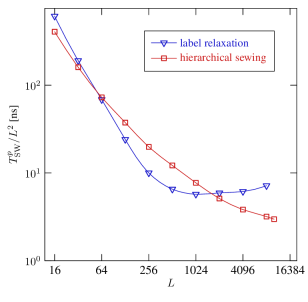
The resulting total run times on the GTX 480 are shown in Fig. 10. The two consolidation approaches lead to quite different size dependence. Tile relaxation results in a rather fast decay of run times per site in the under-utilized regime and is faster than the sewing approach for intermediate system sizes. Eventually, however, the scaling
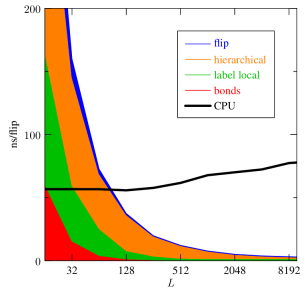
implied by Eqs. (25) and (26) kicks in, which amounts to for , and results in the upturn seen in Fig. 10. For the hierarchical approach, on the other hand, as implied by Eq. (23) the best performance is reached only rather slowly as is increased, but ultimately becomes constant as (theoretically) . At and for the Potts model, SW with sewing performs at ns per spin and per sweep on the GTX 480, while relaxation results in ns per sweep. For the pure cluster identification problem, i.e., without the bond activation and spin flipping steps, these times are reduced to ns and ns, respectively. Figure 11 shows the break down of run times into the algorithmic components of bond activation, labeling on tiles, tile consolidation and spin flipping when using hierarchical sewing. Label consolidation is the dominant contribution up to intermediate system sizes, and only for its run time drops below that of local labeling on tiles. For smaller systems, the fraction of time spent on bond activation and spin flipping is negligible, while (due to the decrease in time spent for label consolidation) it rises to about 20% for . As a reference, Fig. 11 also shows the run time of an optimized, serial CPU implementation using breadth-first search and on-line flipping of spins as the clusters are grown, running on an Intel Core 2 Quad Q6700 at 2.66 GHz.
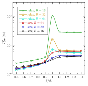
The incipient percolating clusters for the Potts model simulations at are typical for a critical model. For other applications, for instance in image segmentation, it is interesting to investigate the performance for more general situations. Figure 12 displays the run times for an SW update as a function of inverse temperature , comparing the setups with relaxation and hierarchical sewing for tile consolidation. There is a natural increase in run time with the concentration of bonds. While for the sewing procedure, run times increase monotonically with , for the relaxation approach there is a pronounced peak of run times near , where the number of necessary iterations shoots up since now information about the incipient percolating cluster needs to be transmitted across the whole system. Run times become somewhat smaller again for as most bonds crossing tile boundaries belong to the same (percolating) cluster such that, due to concurrency, cluster labels can travel several steps in one iteration. This concurrency effect strongly increases as more tiles are treated simultaneously which, for a fixed number of multiprocessors, is the case for larger tile sizes. Figure 12 shows that the preference of the sewing procedure over relaxation for large systems is robust with respect to variations in temperature and should also be justified for more general structures not resulting from a percolation transition.
| method | CPU | GPU | speedup | |||||
|---|---|---|---|---|---|---|---|---|
| 2 | 1 | self-labeling, relaxation | Q6700 | ns | GTX 480 | ns | ||
| 2 | 1 | self-labeling, sewing | Q6700 | ns | GTX 480 | ns | ||
| 2 | 1 | self-labeling, sewing | Q6700 | ns | GTX 480 | ns | ||
| 2 | 1 | self-labeling, sewing | Q6700 | ns | GTX 580 | ns | ||
| 2 | 1 | self-labeling, sewing | i7@9300 | ns | GTX 580 | ns | ||
| 2 | 1 | self-labeling, sewing | Q6700 | ns | M2070 | ns | ||
| 2 | 1 | self-labeling, sewing | E5620 | ns | M2070 | ns | ||
| 2 | 1 | self-labeling, sewing | E5620 | ns | M2070 | ns | ||
| 2 | 1 | self-labeling, relaxation | Q6700 | ns | GTX 480 | ns | ||
| 2 | self-labeling, sewing | Q6700 | ns | GTX 480 | ns | |||
| 2 | self-labeling, sewing | Q6700 | ns | GTX 480 | ns | |||
| 3 | 1 | self-labeling, sewing | Q6700 | ns | GTX 480 | ns | ||
| 4 | 1 | self-labeling, sewing | Q6700 | ns | GTX 480 | ns | ||
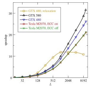
Figure 13 shows the speed-up of the GPU implementation with respect to the CPU code on the Q6700 processor. For large systems, speed-ups in excess of 30 are observed. Comparing different GPU devices, a clear scaling with the number of multiprocessors and global memory bandwidth is observed with the best performance seen for the GTX 580 (, 192 GB/s), followed by the GTX 480 (, 177 GB/s) and the Tesla M2070 (, 144 GB/s). Naturally, effects of higher double-precision floating-point performance of the latter are not seen for the present code, which almost exclusively uses integer and a few single-precision floating point arithmetic instructions. The penalty for activating error correction (ECC) on the memory is minute. Some benchmark results, also including different processors, are collected in Tab. 1.
III Wolff algorithm
For simulations of spin models, Wolff wolff:89a suggested a variant of the Swendsen-Wang algorithm where only a single cluster, seeded at a randomly chosen site, is grown at a time which is then always flipped. Empirically, it is found that this leads to somewhat smaller autocorrelation times than SW wolff:89 ; baillie:91a but, most likely, no change in the dynamical critical exponent (at least for integer ) deng:09 . Conceptually, one can imagine the single-cluster algorithm as a variant of the SW dynamics where after a full decomposition of the lattice according to the SW prescription, a site is picked at random and the cluster of spins it belongs to is flipped. Since the probability of picking a specific cluster in this way is proportional to its size, in this approach larger clusters are flipped on average than in the original SW algorithm. This explains the somewhat reduced autocorrelation times.
While this approach is easily coded in a serial program and, in addition to the smaller autocorrelation times, in a suitable implementation performs at even somewhat less effort per spin than the SW algorithm, it is not straightforwardly parallelized evertz:93 ; bae:95 ; bader:06 ; kaupuzs:10 . The only obvious parallelism lies in the sites at the wave front of the growing cluster, cf. the sketch in Fig. 1. A number of approaches for parallel calculations come to mind:
-
(a)
A full parallel cluster labeling as in SW, followed by picking out and flipping a single cluster. Although many operations are wasteful here, there might still be a speed-up as compared to the serial code. If using a relaxation procedure for label consolidation, this approach can be somewhat improved by modifying the stopping criterion to only focus on the labels belonging to the cluster to be flipped.
-
(b)
Restriction to wave-front parallelism evertz:93 . Due to the rather variable number of sites at the front, however, this generically leads to poor load balancing between the processing units. Load balancing can be improved by a de-localization of the wave front with a “randomized” rearrangement of the lattice. This can be reached, for instance, with a scattered strip partitioning, where strips of the lattice are assigned to available processing units in a round-robin fashion, leading to a more even distribution of sites at the wave front to different processors bae:95 .
-
(c)
Suitable modifications of the single-cluster algorithm to make it more appropriate for parallel computation.
The approach (a) can be easily realized with the techniques outlined in Sec. II. As discussed in Ref. bae:95 , additional load balancing can result in significant improvements on MIMD (multiple instruction, multiple data) machines. It appears less suitable for the mixed architecture of GPUs. In contrast to the more general case of SW dynamics discussed above in Sec. II, I refrain here from a comprehensive evaluation of options, and only give some preliminary results for a modification (c) of the Wolff algorithm appearing suitable for GPU computing.
In this approach, the lattice is again decomposed into tiles of edge length . A single cluster per tile is then grown using a number of threads per tile to operate on the wave front. Unlike the case of the SW implementation, the clusters are not confined to the tiles, but can grow to span the whole lattice. One can easily convince oneself, that the underlying decomposition remains to be the SW one. If seeds in different tiles turn out to belong to the same cluster, different parts of that cluster receive different labels, but since all clusters are flipped the effect is the same as if a single cluster (for that two seeds) had been grown (this is for the case of the model). Logically, this algorithm is identical to performing the full SW decomposition and then selecting points on the lattice, followed by flipping all distinct clusters these points belong to. While this approach satisfies detailed balance (the SW decomposition remains the same and the cluster flipping probability is symmetric), it is not ergodic as it stands since, for instance, it becomes impossible to flip only a single spin. This deficiency can be easily repaired, however, by assigning a flipping probability to the clusters which can be large, but must be strictly smaller than one. If only a relatively small number of tiles is chosen, the decorrelation efficiency of this “few-cluster” variant of the SW algorithm is about the same as that of the single-cluster variant.
For implementing the labeling in tiles, a number of threads per block is chosen. If there are enough pending sites in the queue, each thread is assigned one of these spins which are then examined in parallel. The queue is here realized as a simple linear array of size . This appears inefficient as the size of the wave front will at most be of the order of , where is the fractal dimension of the cluster boundary. In contrast to the use of a ring buffer of length , however, storing in and retrieving from the queue can be realized with atomic operations only cuda , i.e., without the use of locks. Unfortunately, this setup severely limits the range of realizable tile sizes for larger systems as memory requirements for this queue scale as . In contrast to the SW algorithm, bond activation and spin flipping can be done online with the labeling pass. Consequently, the “few-cluster” implementation needs only two kernels, cluster_tile() for the labeling and flipping and reset_inclus() for resetting the cluster labels after each pass. The number of threads per block is adapted to maximize occupancy of the device. In general, it is found that good results are obtained on setting
| (27) |
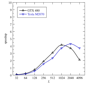
as is the maximum number of threads per block, is the maximum number of active threads and the maximum number of resident blocks per multiprocessor. (Here, denotes the number of multiprocessors of the device.) The resulting speed-ups as compared to a serial code on the Intel Core 2 Quad Q6700 are shown in Fig. 14. The performance for large system sizes is limited by the memory consumption of the queues, limiting the number of tiles. Speed-ups by a factor of up to about five are achieved, significantly lower than for the SW dynamics. It is expected than further optimizations (such as the use of ring buffers instead of queues) could approximately double this speed-up. Nevertheless, for cluster-update simulations on GPUs it might be more efficient to stick with the SW algorithm.
Conclusions
Cluster identification is a pivotal application in scientific computations with applications in the simulation of spin models and percolation, image processing or network analysis. While the underlying problem is inherently non-local in nature, the choice of appropriate algorithms for implementations on GPU allows for significant performance gains as compared to serial codes on CPU. The overall speed-up is seen to be lowest for spin models at criticality, where clusters are fractal and span the system. In all cases, however, speed-ups up to about 30 can be achieved on current GPU devices. This is to be contrasted to the case of purely local algorithms, such as Metropolis simulations of spin models, where speed-ups are seen to be larger by a factor three to five weigel:10c ; weigel:10a ; weigel:11 . Even with this caveat, it seems clear that GPU computing is not limited to the case of purely local problems as significant performance gains can be achieved for highly non-local problems also. Generalizations within the realm of spin-model simulations, such as variants on different lattices or embedded clusters for O() spin models wolff:89a are straightforward.
While the considerations presented here have been restricted to calculations on a single GPU, it should be clear that the approach outlined for the Swendsen-Wang dynamics or the pure cluster identification problem is easily parallelized across several GPUs. For the case of spin-model simulations, the combination of self-labeling and label relaxation appears better suited for this task as for the final spin-flipping step only information local to each GPU is required, whereas for the hierarchical scheme cluster roots (and therefore spin-flipping states) are scattered throughout the whole system. The most effective setup for simulating large systems, therefore appears to be the combination of self-labeling and hierarchical sewing inside of a GPU and label relaxation between GPUs which can easily be realized using MPI with rather low communication overheads.
Acknowledgments
Support by the DFG through the Emmy Noether Programme under contract No. WE4425/1-1 and by the Schwerpunkt für rechnergestützte Forschungsmethoden in den Naturwissenschaften (SRFN Mainz) is gratefully acknowledged.
References
- (1) R. J. Baxter, Exactly Solved Models in Statistical Mechanics (Academic Press, London, 1982)
- (2) K. Binder and D. P. Landau, A Guide to Monte Carlo Simulations in Statistical Physics, 3rd ed. (Cambridge University Press, Cambridge, 2009)
- (3) N. Metropolis, A. W. Rosenbluth, M. N. Rosenbluth, A. H. Teller, and E. Teller, J. Chem. Phys. 21, 1087 (1953)
- (4) R. H. Swendsen and J. S. Wang, Phys. Rev. Lett. 58, 86 (1987)
- (5) U. Wolff, Phys. Rev. Lett. 62, 361 (1989)
- (6) D. Kandel and E. Domany, Phys. Rev. B 43, 8539 (1991)
- (7) N. Kawashima and J. E. Gubernatis, Phys. Rev. E 51, 1547 (1995)
- (8) R. Opara and F. Wörgötter, Neural Comput. 10, 1547 (Aug. 1998)
- (9) X. Wang and J. Zhao, International Conference on Natural Computation 7, 352 (2008)
- (10) D. Stauffer and A. Aharony, Introduction to Percolation Theory, 2nd ed. (Taylor & Francis, London, 1994)
- (11) J. Hoshen and R. Kopelman, Phys. Rev. B 14, 3438 (Oct. 1976)
- (12) F. Belletti, M. Cotallo, A. Cruz, L. A. Fernández, A. G. Guerrero, M. Guidetti, A. Maiorano, F. Mantovani, E. Marinari, V. Martín-Mayor, A. Muñoz Sudupe, D. Navarro, G. Parisi, S. P. Gaviro, M. Rossi, J. J. Ruiz-Lorenzo, S. F. Schifano, D. Sciretti, A. Tarancón, and R. L. Tripiccione, Comput. Sci. Eng. 11, 48 (2009)
- (13) H. W. J. Blöte, L. N. Shchur, and A. L. Talapov, Int. J. Mod. Phys. C 10, 1137 (1999)
- (14) J. D. Owens, M. Houston, D. Luebke, S. Green, J. E. Stone, and J. C. Phillips, Proceedings of the IEEE, Proceedings of the IEEE 96, 879 (May 2008)
- (15) D. B. Kirk and W. W. Hwu, Programming Massively Parallel Processors (Elsevier, Amsterdam, 2010)
- (16) T. Preis, P. Virnau, W. Paul, and J. J. Schneider, J. Comput. Phys. 228, 4468 (2009)
- (17) M. Bernaschi, G. Parisi, and L. Parisi, Comput. Phys. Commun. 182, 1265 (Jun. 2011)
- (18) M. Weigel, “Performance potential for simulating spin models on GPU,” (2011), preprint arXiv:1101.1427
- (19) E. E. Ferrero, J. P. De Francesco, N. Wolovick, and S. A. Cannas, “-state Potts model metastability study using optimized GPU-based Monte Carlo algorithms,” (Jan. 2011), preprint arXiv:1101.0876, arXiv:1101.0876
- (20) M. Weigel, Comput. Phys. Commun. 182, 1833 (2011)
- (21) M. Weigel and T. Yavors’kii, Physics Procedia(2011), in print
- (22) D. Heermann and A. N. Burkitt, Parallel Comput. 13, 345 (1990)
- (23) C. F. Baillie and P. D. Coddington, Concurrency: Pract. Exper. 3, 129 (1991)
- (24) H. Mino, Comput. Phys. Commun. 66, 25 (1991)
- (25) J. Apostolakis, P. Coddington, and E. Marinari, Europhys. Lett. 17, 189 (Jan. 1992)
- (26) G. T. Barkema and T. MacFarland, Phys. Rev. E 50, 1623 (Aug. 1994)
- (27) M. Bauernfeind, R. Hackl, H. G. Matuttis, J. Singer, T. Husslein, and I. Morgenstern, Physica A 212, 277 (1994)
- (28) M. Flanigan and P. Tamayo, Physica A 215, 461 (1995)
- (29) J. Martín-Herrero, J. Phys. A 37, 9377 (2004)
- (30) “CUDA zone — Resource for C developers of applications that solve computing problems,” http://www.nvidia.com/object/cuda_home_new.html
- (31) F. Y. Wu, Rev. Mod. Phys. 54, 235 (1982)
- (32) C. M. Fortuin and P. W. Kasteleyn, Physica 57, 536 (1972)
- (33) C. K. Hu, Phys. Rev. B 29, 5103 (1984)
- (34) A. Coniglio and W. Klein, J. Phys. A 13, 2775 (1980)
- (35) X. J. Li and A. D. Sokal, Phys. Rev. Lett. 63, 827 (Aug. 1989)
- (36) Y. Deng, T. M. Garoni, J. Machta, G. Ossola, M. Polin, and A. D. Sokal, Phys. Rev. Lett. 99, 055701 (Jul. 2007)
- (37) I do not take the effects of latency hiding and other scheduling specificities into account in the scaling formulae, but discuss them in some places in connection with observed deviations from these simplified laws. It is also assumed that the number of threads per block is at least since due to the limitation to eight active blocks per multiprocessor on current NVIDIA GPUs, there would otherwise be idle cores.
- (38) M. Matsumoto and T. Nishimura, ACM Trans. Model. Comput. Simul. 8, 3 (Jan. 1998)
- (39) J. E. Gentle, Random number generation and Monte Carlo methods, 2nd ed. (Springer, Berlin, 2003)
- (40) A. E. Ferdinand and M. E. Fisher, Phys. Rev. 185, 832 (1969)
- (41) T. H. Cormen, C. E. Leiserson, R. L. Rivest, and C. Stein, Introduction to Algorithms, 3rd ed. (MIT Press, 2009) ISBN 9780262533058
- (42) D. A. Bader and K. Madduri, in Proc. The 35th International Conference on Parallel Processing (ICPP) (Columbus, Ohio, 2006) pp. 523–530
- (43) R. E. Tarjan, J. ACM 22, 215 (Apr. 1975)
- (44) M. E. J. Newman and R. M. Ziff, Phys. Rev. E 64, 016706 (2001)
- (45) H. J. Herrmann and H. E. Stanley, J. Phys. A 21, L829 (Sep. 1988)
- (46) E. Miranda, Physica A 175, 229 (Jul. 1991)
- (47) Note that this still leads to some under-utilization of the device due to the limit of eight active blocks per multiprocessor which requires at least four threads per block for full occupancy with blocks.
- (48) U. Wolff, Phys. Lett. B 228, 379 (1989)
- (49) C. F. Baillie and P. D. Coddington, Phys. Rev. B 43, 10617 (May 1991)
- (50) Y. Deng, X. Qian, and H. W. J. Blöte, Phys. Rev. E 80, 036707 (Sep. 2009)
- (51) H. G. Evertz, J. Stat. Phys. 70, 1075 (Feb. 1993)
- (52) S. Bae, S. H. Ko, and P. D. Coddington, Int. J. Mod. Phys. C 6, 197 (1995)
- (53) J. Kaupužs, J. Rimšans, and R. V. N. Melnik, Phys. Rev. E 81, 026701 (Feb. 2010)