On Real Time Coding with Limited Lookahead

Abstract

A real time coding system with lookahead consists of a memoryless source, a memoryless channel, an encoder, which encodes the source symbols sequentially with knowledge of future source symbols upto a fixed finite lookahead, $d$, with or without feedback of the past channel output symbols and a decoder, which sequentially constructs the source symbols using the channel output. The objective is to minimize the expected per-symbol distortion.

For a fixed finite lookahead $d\geq 1$ we invoke the theory of controlled markov chains to obtain an average cost optimality equation (ACOE), the solution of which, denoted by $D(d)$, is the minimum expected per-symbol distortion. With increasing $d$, $D(d)$ bridges the gap between causal encoding, $d=0$, where symbol by symbol encoding-decoding is optimal and the infinite lookahead case, $d=\infty$, where Shannon Theoretic arguments show that separation is optimal.

We extend the analysis to a system with finite state decoders, with or without noise-free feedback. For a Bernoulli source and binary symmetric channel, under hamming loss, we compute the optimal distortion for various source and channel parameters, and thus obtain computable bounds on $D(d)$. We also identify regions of source and channel parameters where symbol by symbol encoding-decoding is suboptimal. Finally, we demonstrate the wide applicability of our approach by applying it in additional coding scenarios, such as the case where the sequential decoder can take cost constrained actions affecting the quality or availability of side information about the source.

I Introduction

I-A Motivation and Related Work

A memoryless source $\{U_{1},U_{2},\ldots\}$ is to be communicated over a memoryless channel with the objective of minimizing expected average (per-symbol) distortion, with or without the availability of unit-delay noise-free feedback. The communication is in real time and hence the encoding and decoding is sequential, with a fixed finite lookahead of source symbols available at the encoder (cf. the setting in Fig. 1). The motivation stems from practical systems such as for video streaming, cache memory devices in computing systems, real time communication systems etc., where the encoder has a fixed buffer of future source symbols, and the quality of service demands that encoding and decoding should be in real time. The problem finds its applications in other sequential decision systems, where resource allocation should be done on the fly due to adverse effects of latency or delay, such as sensor networks, weather-monitoring systems, flow in societal networks such as transportation networks, recycling systems, etc. A natural criterion of performance is to minimize the expected average distortion. What is the best we can do here ? Note that such a framework with real time constraints is not covered by Shannon Theory. In classical Information Theory, encoding of long “typical” sequences in blocks as well as block decoding introduces large delays and thus such achievable schemes violate the very premise of bounded or no delay constraint. To answer the question, we invoke markov decision theory and cast our problem and other such variants as discrete time controlled markov chains with average cost criterion.

The problem is well motivated by practical problems of delay constrained source-channel coding and has been of much interest in the literature. There have also been many different ways to model the notion of sequential encoding and decoding. In the source coding context, causal source codes were studied in [1], [2], [3], which demand the reconstruction to depend causally on the source symbols. But this is a much weaker constraint and causal source codes can operate on large delays as was pointed out in [1] itself. Causal source codes with side information were studied in [4].

Note that we can transform our setting of limited encoder lookahead of $d$, to that of a zero lookahead of a markov source, $V_{i}=U_{i}^{i+d}$. This transformation puts the problem in the class of sequential encoding decoding problems with markov sources. When the communication horizon is fixed, the structure of optimal encoding and decoding policies with Markov sources have been studied in [5], [6], [7], [8], [9], [10]. In [11], authors propose a systematic methodology for such a non-classical information structure to search for an optimal strategy.

The problem of real time coding and decoding in semi stochastic setting, i.e., for the individual sequences was studied in [12] and [13], while finite state digital systems were the subject of study in [14].

The connection between dynamic programming and information theory has been well exploited. The problem of computing the capacity of channels with feedback was formulated as a Markov Decision Process in [15], [16]. The long standing problem of capacity of trapdoor channel (cf. [17], [18]) with feedback was evaluated using average cost optimality equations in [19]. Zero error capacity for certain channel coding problems was computed using dynamic programming in [20].

I-B Contributions and Organization of the Paper

The approaches in [5], [6], [7], [8], [9], [10] and [11] are inspired by control theory, which provides tools for finding optimal schemes and understanding their structure. In this work, we take these tools further to provide more explicit expressions and bounds for the optimum performance under a given lookahead constraint $d$. While optimum performance in the case $d=0$ is easily shown to be attained by “symbol-by-symbol” operations, and the case $d=\infty$ can be answered with the tools of Shannon theory, for any finite $d\geq 1$, the existing literature does not provide useful analytical values or bounds on the minimum expected average distortion, $D(d)$. In addition to being amenable to a decision theoretic formulation of Markov sources, as in the surveyed literature above, the model we consider here is more basic and lends itself to simpler average cost optimality equation, which in some cases (cf. Section V) can be computed exactly. While in [7], [8], [10] emphasis is on expected total fixed horizon cost, we argue that expected average cost over infinite horizon is a more natural criterion of performance as in the sequential encoding and decoding problems, we typically do not know when to stop, and hence we would like to analyze the asymptotics of the horizon-independent problem. While the main focus in this work has been to characterize the minimum achievable distortion, the average cost optimality equations also characterize sufficient conditions on the optimality of stationary (encoding and decoding) policies.

Note that in our communication problem in Fig. 1, the lookahead is available only at the encoder while the decoder constructs the estimates causally, instead of a seemingly more general setting where lookahead of $l_{e}$ is present at the encoder while decoder has lookahead $l_{d}$. However performance of any policy/code with encoder and decoder lookahead parameters $(l_{e},l_{m})$ can be attained arbitrarily closely by the optimal policy for our setting in Fig. 1 with $d=l_{e}+l_{m}$ as pointed out in Section II of [13]. Authors in [21] consider the communication problem similar to our setting with $l_{e}=0$, $l_{d}=d$ for $d\geq 0$, per-symbol distortion $D(d)$ and show that $D(d)$ converges exponentially rapidly to $D(\infty)$ and provide bounds on the exponent. However the results are asymptotic in nature and hence different from this work, which is explicit exact or approximate characterization of values for $D(d)$ for any fixed, possibly small $d$.

Recently there has been work in the direction of “action in information theory” , i.e. canonical Shannon theoretic models with encoder and/or decoder taking cost constrained actions to affect the generation or availability of channel state information, side information, feedback etc., cf. action in point to point scenarios in [22], [23], [24] [25], [26] and in multi-terminal systems in [27], [28]. We revisit the setting of source coding with a side information vending machine, as in [22] (See Fig. 6) for the case where the encoding is sequential with lookahead, decoder takes an action $A_{v}$ sequentially dependent on the encoded symbols to get side information about the source through a memoryless channel, $P_{Y|U,A_{v}}$. The reconstruction of the source is based upon the current encoded symbol, the current side information symbol and memories storing the past encoded symbols and side information symbols. We show that the problem can be formulated as a constrained Markov Decision Process.

The main contribution of this paper is the casting of a large class of limited delay source, channel and joint source-channel coding problems in the realm of sequential decision theory, obtain characterizations of the optimum performance via average cost optimality equations with finite or compact state spaces, and solve exactly or obtain bounds for the expected average distortion as a function of lookahead $d$.

The paper is organized as follows. Section II describes the basic model of problems with lookahead (See Fig. 1), encoding is sequential using the lookahead and unit delay noise-free feedback, $X_{i}(U^{i+d},Y^{i-1})$, while the decoding depends on the current channel output and the past memory, $\hat{U}_{i}(Y_{i},Z_{i-1})$. The memory evolves as $Z_{i}(Z_{i-1},Y_{i})$. We seek to find the minimum expected average distortion as a function of lookahead, i.e.,

$$D(d)=\inf_{\{X_{i}(\cdot)\},\{\hat{U}_{i}(\cdot)\}}\limsup_{N\rightarrow\infty}\mathsf{E}\left[\frac{1}{N}\sum_{i=1}^{N}\Lambda(U_{i},\hat{U}_{i})\right].$$ (1)

In Section III we present an overview of controlled markov processes with average cost, the unconstrained case in Section III-A and constrained control in Section III-B. Section IV studies the case of complete memory, i.e., $Z_{i}=Y^{i}$. In Section IV-A we use the theory of Section III to construct an average cost optimality equation, the solution to which is the average optimal distortion. In Section IV-B, we consider the question “to look or not to lookahead ” and specify a sufficient condition under which symbol by symbol encoding-decoding is optimal for a given source, channel, distortion function and lookahead. This kind of result in our problem of sequential encoding decoding with lookahead complements that of “to code or not to code ” of [29]. In Section V, we consider the framework with finite state decoders, constructing corresponding ACOE in Section V-A. In Section V-B, we use relative value iteration to solve the problem exactly for an example of binary source and binary symmetric channel under hamming loss, thereby demonstrating how the average distortion values for this setting can be used to bound $D(d)$ of Section IV. We also contrast with the extreme cases of no lookahead, $d=0$, where symbol by symbol policies are optimal and $d=\infty$ where Shannon’s Separation Theorem [30] determines the minimum expected average distortion. We also highlight the regions of source-channel parameters where for any finite $d\geq 1$, symbol by symbol encoding-decoding is strictly suboptimal for a Bernoulli source and binary symmetric channel. Section VI relaxes the assumption of the previous sections that feedback is present. In Section VII, the setting of source coding with a side information vending machine is considered. Here again, encoding is sequential with lookahead, decoder takes cost constrained actions, $A_{v,i}$, sequentially to get side information about the source through a memoryless channel, $P_{Y|U,A_{v}}$. The decoding is the optimal reconstruction $\hat{U}_{i}(X_{i},Y_{i},M_{i-1},N_{i-1})$, where $M_{i-1}$ and $N_{i-1}$ are the memories storing some or all of past encoded symbols and side information symbols, respectively. Section VII-A evaluates the case when encoder also has access to the side information, with decoder having complete memory in Section VII-A1, while finite memory decoders are considered in Section VII-A2. Section VII-B studies the same source coding problem with a side information vending machine but now encoder has no access to side information. Section VIII summarizes the methodology developed in this paper of constructing average cost optimality equations. The paper is concluded in Section IX.

II Problem Formulation

We begin by explaining the notation to be used throughout this paper. Let upper case, lower case, and calligraphic letters denote, respectively, random variables, specific or deterministic values which random variables may assume, and their alphabets. For two jointly distributed random variables, $X$ and $Y$, let $P_{X}$, $P_{XY}$ and $P_{X|Y}$ respectively denote the marginal of $X$, joint distribution of $(X,Y)$ and conditional distribution of $X$ given $Y$. $X_{m}^{n}$ is a shorthand for the $n-m+1$ tuple $\{X_{m},X_{m+1},\cdots,X_{n-1},X_{n}\}$. $\mathcal{B}(\mathcal{X})$ denotes the Borel $\sigma$-algebra of a given topological space, $\mathcal{X}$. $\mathcal{P}(\mathcal{X})$ denotes the probability simplex on the finite alphabet, $\mathcal{X}$. $C_{b}(\mathcal{X})$ denotes the set of continuous and bounded functions on the topological space $\mathcal{X}$. ${\bf 1}_{\{\cdot\}}$ stands for the indicator function. $\mathbf{N}$ and $\mathbf{R}$ denote the sets of natural and real numbers respectively. We impose the assumption of finiteness of cardinality on all alphabets of operational significance (source, channel input, channel output, reconstruction), unless otherwise indicated.

Figure 1: Real time coding with lookahead. Encoder uses future source symbols upto a fixed finite lookahead, $d$ and unit-delay noise free feedback, decoder uses present channel output and past memory for source reconstruction. Complete memory case corresponds to $Z_{i}=Y^{i}$ which implies $\left|\mathcal{Z}_{i}\right|=\left|\mathcal{Y}\right|^{i}$.

The general problem setup, depicted in Fig. 1 consists of the following principle components :

• Source : Generates i.i.d. source symbols, $\{U_{i}\}_{i\in\mathbf{N}}\in\mathcal{U}$. The source symbols are distributed $\sim P_{U}$.

• Channel Encoder : The encoder has access to unit-delay noise-free feedback from the channel output and future source symbols upto a fixed finite lookahead, $d$, i.e, $X_{i}=f_{e,i}(U^{i+d},Y^{i-1})$, where $f_{e,i}$ is the encoding function, $f_{e,i}:\mathcal{U}^{i+d}\times\mathcal{Y}^{i-1}\rightarrow\mathcal{X}$, $i\in\mathbf{N}$.

• Channel : Given channel input symbol, $x_{i}$, and all the source symbols and past channel inputs and outputs, $(u_{1}^{\infty},x^{i-1},y^{i-1})$, channel output, $y_{i}$ is distributed i.i.d. $\sim P_{Y|X}$, i.e.,

  $$P(y_{i}|u_{1}^{\infty},x^{i},y^{i-1})=P_{Y|X}(y_{i}|x_{i}).$$ (2)

• Memory : The decoder cannot make use of all the channel output symbols upto current time due to memory constraints. Memory is updated as a function of the past state of the memory and the current channel output, i.e., $Z_{i}=f_{m,i}(Z_{i-1},Y_{i})$, where the $f_{m.i}$ is the memory update function, $f_{m,i}:\mathcal{Z}_{i-1}\times\mathcal{Y}\rightarrow\mathcal{Z}_{i}$, $i\in\mathbf{N}$. Note that the alphabet $\mathcal{Z}_{i}$ can grow with $i$, hence the setup also includes the special case of complete memory, i.e., $Z_{i}=Y^{i}$ which implies $\left|\mathcal{Z}_{i}\right|=\left|\mathcal{Y}\right|^{i}$.

• Channel Decoder : Channel decoder uses the current channel output and the past memory state to construct its estimate of the source symbol, i.e., $\hat{U}_{i}=f_{d,i}(Z_{i-1},Y_{i})$, the decoding rule is the map, $f_{d,i}:\mathcal{Z}_{i-1}\times\mathcal{Y}\rightarrow\hat{\mathcal{U}}$.

The alphabets $\mathcal{U}$, $\mathcal{X}$, $\mathcal{Y}$ and $\hat{\mathcal{U}}$ are assumed to be finite. Let $\Lambda(\cdot,\cdot):\mathcal{U}\times\hat{\mathcal{U}}\rightarrow\mathbf{R}$ indicate a distortion function. We assume for simplicity that, $0\leq\Lambda(\cdot,\cdot)\leq\Lambda_{max}<\infty$. Let the tuple $\mu(d)=(f_{e},f_{m},f_{d})$ indicate the sequence of encoding rules, $\{f_{e,i}\}_{i\in\mathbf{N}}$, memory update rules, $\{f_{m,i}\}_{i\in\mathbf{N}}$ and decoding rules, $\{f_{d,i}\}_{i\in\mathbf{N}}$.

Definition 1

[Distortion-Optimal Policy] For a fixed lookahead, $d$, we define $d$-distortion optimal policies, $\mathcal{P}^{opt}(d)$ as the set of $(f_{e},f_{m},f_{d})$-policies, denoted by $\mu(d)$, which achieve the minimum expected average distortion, i.e,

$$\mathcal{P}^{opt}(d)=\left\{\mu(d):\mu(d)=\arg\inf_{\{f_{e},f_{m},f_{d}\}}\limsup_{N\rightarrow\infty}\mathsf{E}\left[\frac{1}{N}\sum_{i=1}^{N}\Lambda(U_{i},\hat{U}_{i})\right]\right\}.$$ (3)

The corresponding minimum expected distortion as a function of lookahead, $d$,

$$D(d)=\inf_{\{f_{e},f_{m},f_{d}\}}\limsup_{N\rightarrow\infty}\mathsf{E}\left[\frac{1}{N}\sum_{i=1}^{N}\Lambda(U_{i},\hat{U}_{i})\right].$$ (4)

Our main goal is to characterize $D(d)$ and identify structural properties of the elements of $\mathcal{P}^{opt}(d)$.

Note 1

Note that $\inf$ in the definition of $D(d)$ can equivalently be replaced by $\min$ (cf. Appendix A). This implies that $\mathcal{P}^{opt}(d)$ is non-empty. Taking limsup in definition of $D(d)$, while appearing more conservative, is actually inconsequential as you would get the same value of D(d) if you put a liminf in the definition. This can be easily argued as follows. Let, the per-symbol expected distortion under a policy $\mu$ upto time $N$ be denoted by $D_{\mu}^{(N)}$. Denoting $D^{\sup}(d)$ and $D^{\inf}(d)$ as the distortion criterion with $\limsup$ and $\liminf$ respectively, we know $D^{\inf}(d)\leq D^{\sup}(d)$. We will now show $D^{\inf}(d)\geq D^{\sup}(d)$. Let a policy $\mu^{\ast}$ attains the infimum for $D^{\inf}(d)$ (that there exists such policy follows from the same arguments as above for the non-emptiness of $\mathcal{P}^{opt}(d)$). This implies (as $\Lambda(\cdot)$ is bounded) for $\epsilon>0$, $\exists$ $N(\epsilon)>0$ such that under this policy $D^{(N(\epsilon))}\leq D^{\inf}(d)+\epsilon$. Operating such a policy in $b$ blocks,

$$D^{\sup}(d)\leq\lim_{b\rightarrow\infty}D_{\mu^{\ast}}^{(N(\epsilon)b)}\leq D^{\inf}(d)+\epsilon,$$ (5)

which implies in the limit $\epsilon\rightarrow 0$, $D^{\sup}(d)\leq D^{\inf}(d)$.

III Controlled Markov Process with Average Cost : Background and Preliminaries

We present here an overview of parts of the controlled Markov process with average cost criterion framework that will be applied. First, we present an overview of the unconstrained case where the only objective is to maximize an expected average cost. We then consider the constrained case where, in addition, the system needs to satisfy certain expected average cost constraints.

III-A Unconstrained Control

Here we overview results about general Borel state and action spaces. We refer to [31] for a more complete discussion. The problem is characterized by the tuple $(\mathcal{S},A_{s},\mathcal{A},\mathcal{W},F,P_{S},P_{W},g)$ and a discrete time dynamical system,

$$s_{t}=F(s_{t-1},a_{t},w_{t}),$$ (6)

where the states $s_{t}$ take values in finite, countable or in general Borel space $\mathcal{S}$ (called the state space), actions $a_{t}$ take values in the admissible action space, $A_{s}(s_{t})$ which is a subset of a compact subset $\mathcal{A}$ (called the action space) of a Borel space, and the disturbance, $w_{t}$, takes values in a measurable space $\mathcal{W}$ (called the disturbance space). Initial state $S_{0}$ is drawn with distribution $P_{S}$ and the disturbance $w_{t}$ is drawn from the distribution, $P_{W}(\cdot|s_{t-1},a_{t})$ which depends on past actions and states, only through the pair $(s_{t-1},a_{t})$. We consider only measurable functions. A policy $\pi$ is defined to be the sequence of functions, $\pi=(\mu_{1},\mu_{2},\cdots)$, where $\mu_{t}$ is the function which maps histories ($\phi_{t}=(s_{0},w_{0},\cdots,w_{t-1})$) to actions. A set of history deterministic policies, $\Pi_{HD}$ is characterized by policies for which actions are generated as $a_{t}=\mu_{t}(\Phi_{t})$. A set of Markov deterministic policies, $\Pi_{MD}$ is characterized by policies for which actions are generated as $a_{t}=\mu_{t}(s_{t-1})$. A set of policies $\Pi_{SD}$ is referred to as stationary deterministic if it is characterized by a function $\mu:\mathcal{S}\rightarrow\mathcal{A}$ such that, $\mu_{t}(\Phi_{t})=\mu(s_{t-1})$ $\forall\ t$. Policies can be randomized or deterministic ([31], Section 2.2). The policy sets $\Pi_{HR}$, $\Pi_{MR}$ and $\Pi_{SR}$ respectively stand for history randomized, markov randomized and stationary randomized policies. As per our definitions and interests, the largest class of policies considered henceforth will be history deterministic policies, $\Pi_{HD}$. Let

$$\mathcal{K}=\{(x,a):x\in\mathcal{S},a\in A_{s}(x)\}\in\mathcal{B}(\mathcal{S}\times\mathcal{A}).$$ (7)

Note if $\mathcal{S}$ and $\mathcal{A}$ are compact subsets of a Borel space, $\mathcal{K}$ is a compact subset $\in\mathcal{B}(\mathcal{S}\times\mathcal{A})$. The dynamics induce a stochastic transition kernel on $\mathcal{B}(\mathcal{S})\times\mathcal{K}$, $Q(\cdot|x,a)$, which implies for each $(x,a)\in\mathcal{K}$, $Q(\cdot|x,a)$ is probability measure on $\mathcal{B}(\mathcal{S})$ and for each $D\in\mathcal{B}(\mathcal{S})$, $Q(D|\cdot)$ is Borel measurable on $\mathcal{K}$.
The objective is to maximize expected average reward given a bounded one stage reward function, $g:\mathcal{K}\rightarrow\mathbf{R}$ and find the optimal policy. The average reward of a policy $\pi$ with a given initial state distribution $\nu$ is defined by,

$$J({\nu,\pi})\stackrel{{\scriptstyle\triangle}}{{=}}\liminf_{N\rightarrow\infty}\mathsf{E}^{\pi}_{\nu}\left[\frac{1}{N}\sum_{t=1}^{N}g(S_{t-1},\mu_{t}(\Phi_{t}))\right].$$ (8)

The optimal average reward and the optimal policy is defined by,

$$J^{opt}(\nu) = \sup_{\pi}J({\nu,\pi})$$ (9)

$$\pi^{opt}(\nu) = \{\pi:J({\nu,\pi})=J^{opt}(\nu)\}.$$ (10)

Note that in general for a controlled Markov process with average cost criterion, where the state space is infinite, the total expected average cost might depend on the initial state. However, operationally, since our objective is to minimize the expected average distortion as in Eq. 4, we can decide to start of the system with the best initial state, state which yields the best distortion, in which case the optimal cost and optimal policy will be denoted by, $J^{opt}$ and $\pi^{opt}$.

$$J^{opt} = \sup_{\nu}J^{opt}({\nu})$$ (11)

$$\pi^{opt} = \{\pi:\exists\ \nu\mbox{ s.t. }J(\nu,\pi)=J^{opt}\}.$$ (12)

We need not dwell on sensitivity of the optimal cost to initial states, as this will not be an issue in our application of this framework. However when state space is say finite, irreducible and positive recurrent, average cost is indeed equal for all initial states. In general, there can be more than one optimal policy, in which case ties are resolved arbitrarily.
The following theorem describes the average cost optimality equation (ACOE) for such a process, and relates the optimal reward with the optimal stationary deterministic policy.

Theorem 1 (cf. Theorem 6.1 of [31])

If $\lambda\in\mathbf{R}$ and a bounded function $h:\mathcal{S}\rightarrow\mathbf{R}$ satisfy,

$$\lambda+h(s)=\sup_{a\in\mathcal{A}}\left[g(s,a)+\int P_{W}(dw|s,a)h(F(s,a,w))\right],\mbox{ }\forall\ s\in\mathcal{S},$$ (13)

then $\lambda=J^{opt}$. Further, if there is a function $\mu:\mathcal{S}\rightarrow\mathcal{A}$ such that $\mu(s)$ attains the supremum above for all states, then $J({\pi})=J^{opt}$ for $\pi=\{\mu_{1},\mu_{2},\cdots\}$ with $\mu_{i}(\Phi_{i})=\mu(s_{i-1})$, $\forall i$.

Note 2

As in [31], the above theorem assumes the conditions of semi-continuous model, ([31], Section 2.4). However in the set of problems considered in our paper, all such assumptions will be trivially met such as the transition kernel being weakly continuous in $\mathcal{K}$ and the continuity of $g$. For brevity, we omit explicitly mentioning such assumptions before invoking the above theorem in the sections to follow.

III-B Constrained Control

In constrained control, the system is characterized by the tuple $(\mathcal{S},A_{s},\mathcal{A},\mathcal{W},F,P_{S},P_{W},g,\mathbf{l},\mathbf{\Gamma})$. With all the terms carrying the same meaning as in previous subsection, $\mathbf{l}=\{l_{1}(\cdot),\cdots,l_{k}(\cdot)\}$ and $\mathbf{\Gamma}=\{\Gamma_{1},\cdots,\Gamma_{k}\}$ are respectively $k$-dimensional constraint functions (defined on $\mathcal{K}$) and cost vectors for some $k\in\mathbf{N}$. the dynamics of the system are precisely the same as in the unconstrained case, the objective here being,

$$\mathbf{maximize}\mbox{ } J(\nu,\mu)$$

$$\mathbf{subject}\mbox{ }\mathbf{to}\mbox{ } J^{c}_{i}(\nu,\mu)\leq\Gamma_{i}\mbox{ }\forall\mbox{ }i=1,\cdots,k,$$ (14)

where,

$$J({\nu,\pi})\stackrel{{\scriptstyle\triangle}}{{=}}\liminf_{N\rightarrow\infty}\mathsf{E}^{\pi}_{\nu}\left[\frac{1}{N}\sum_{t=1}^{N}g(S_{t-1},\mu_{t}(\Phi_{t}))\right],$$ (15)

is the average cost and,

$$J_{i}^{c}({\nu,\pi})\stackrel{{\scriptstyle\triangle}}{{=}}\liminf_{N\rightarrow\infty}\mathsf{E}^{\pi}_{\nu}\left[\frac{1}{N}\sum_{t=1}^{N}l_{i}(S_{t-1},\mu_{t}(\Phi_{t}))\right]\mbox{ }\forall\mbox{ }i=1,\cdots,k,$$ (16)

are the constraints. [31] and [32] provide a treatment of this problem but only for denumerable states. We here present the more general framework of [33], with compact state and action spaces. The Lagrangian, $L$, associated with the problem is defined as,

$$L((\nu,\pi),\lambda)=J(\nu,\pi)+\sum_{i=1}^{k}\lambda_{i}(\Gamma_{i}-J_{i}^{c}(\nu,\mu)),$$ (17)

for any $(\nu,\pi)\in P(\mathcal{S})\times\Pi_{HD}$ and $\lambda=(\lambda_{1},\cdots,\lambda_{k})\in\mathbf{R}^{k}_{+}$ (positive orthant of the $k$-dimensional Euclidean space).

The following theorem gives conditions of optimality of a particular initial state distribution and a policy.

Theorem 2

[Theorem 2.3 of [33]] Assume the following conditions for the tuple $(\mathcal{S},A_{s},\mathcal{A},\mathcal{W},F,P_{S},P_{W},g,\mathbf{l},\mathbf{\Gamma})$,

• $\mathcal{S}$ and $\mathcal{K}$ are compact.

• $g\in C_{b}(\mathcal{K})$ and $l_{i}\in C_{b}(\mathcal{K}),\mbox{ }\forall\mbox{ }i=1,\cdots,k$.

• For all $x_{n}\rightarrow x$ and $a_{n}\rightarrow a$, $Q(\cdot|x_{n},a_{n})$, converges weakly to $Q(\cdot|x,a)$.

• (Slater’s Condition) There exists a $(\overline{\nu},\overline{\pi})\in P(\mathcal{S})\times\Pi_{HD}$ such that,

  $$J_{i}^{c}(\overline{\nu},\overline{\pi})<\Gamma_{i}\mbox{ }\forall\mbox{ }i=1,\cdots,k.$$ (18)

Under the conditions C1-C4, the Lagrangian $L(\cdot,\cdot)$ has a saddle point with a randomized stationary policy, i.e., $\exists\mbox{ }\lambda^{\ast}\geq 0$ and $(\nu^{\ast},\pi^{\ast})\in P(\mathcal{S})\times\Pi_{SR}$ such that,

$$L((\nu,\pi),\lambda^{\ast})\leq L((\nu^{\ast},\pi^{\ast}),\lambda^{\ast})\leq L((\nu^{\ast},\pi^{\ast}),\lambda),\mbox{ }\forall\mbox{ }(\nu,\pi)\in P(\mathcal{S})\times\Pi,\mbox{ }\lambda\geq 0,$$ (19)

which implies (from Theorem 2.1 of [33]) that $(\nu^{\ast},\pi^{\ast})$ is a constrained optimal pair. Further (Theorem 2.2 of [33]),

$$L^{\ast}=L((\nu^{\ast},\mu^{\ast}),\lambda^{\ast})=\inf_{\lambda\geq 0}\sup_{(\nu,\pi)\in P(\mathcal{S})\times\Pi_{HD}}L((\nu,\pi),\lambda)=\sup_{(\nu,\pi)\in P(\mathcal{S})\times\Pi_{HD}}\inf_{\lambda\geq 0}L((\nu,\pi),\lambda),$$ (20)

and $L^{\ast}$ is the solution of the problem or the minimum expected average distortion such that the constraints are satisfied.

Note 3

In all the settings considered henceforth, $\forall\ s\in\mathcal{S}$, $A_{s}(s)=\mathcal{A}$, hence with benign abuse of notation, we will drop $A_{s}$ from the tuple associated with our description.

IV Real-Time Coding with Limited Lookahead : Complete Memory

The problem we described in Section II (Fig. 1) is an abstraction of a real time communication problem with the encoder having a fixed lookahead of the future source symbols and a perfect unit-delay feedback of the channel output symbols. In this section, we show that this problem can be formulated as a controlled Markov chain process with average cost criterion, and derive an optimality equation. Before that, we modify our source to concentrate on an equivalent problem. Note that the i.i.d. source, $S=\{U_{i}\}_{i\in\mathbf{N}}$ considered can be replaced by a markov source $S_{M}=\{V_{i}\}_{i\in\mathbf{N}}$ such that, $V_{i}=U_{i}^{i+d}\in\mathcal{U}^{d+1}$. Since the source $S$ is i.i.d., the transition kernel for this Markov process $S_{M}$ from $v=(u_{1},u_{2},\cdots,u_{d+1})$ to $\tilde{v}=(\tilde{u}_{1},\tilde{u}_{2},\cdots,\tilde{u}_{d+1})$ is given by,

$$K(v,\tilde{v})=P(\tilde{v}|v)={\bf 1}_{\{(u_{2},\cdots,u_{d+1})=(\tilde{u}_{1},\cdots,\tilde{u}_{d})\}}P_{U}(\tilde{u}_{d+1}).$$ (21)

The transition matrix is denoted by $\mathbf{K}$. Let us assume the distribution of initial state is $P_{V}$. Also there is no loss of optimality in considering encoding functions to be $\left|\mathcal{V}\right|$ dimensional mappings, $\{f_{e,i}(v,V^{i-1},Y^{i-1})\}_{v\in\mathcal{V}}$. The effective problem with modified source, $S_{M}$ is now a real-time communication problem as in Fig. 2 with no lookahead. For this modified problem, we seek to minimize the average reward,

$$\inf\limsup_{n\rightarrow\infty}\frac{1}{n}\mathsf{E}\left[\sum_{i=1}^{n}\tilde{\Lambda}(V_{i},\hat{V}^{opt}_{i}(Y^{i}))\right]=\inf\limsup_{n\rightarrow\infty}\frac{1}{n}\mathsf{E}\left[\sum_{i=1}^{n}\Lambda(U_{i},\hat{U}^{opt}_{i}(Y^{i}))\right],$$ (22)

where $\tilde{\Lambda}(V_{i},\hat{V}^{opt}_{i}(Y^{i}))=\Lambda(U_{i},\hat{U}^{opt}_{i}(Y^{i}))$. In this section we construct an average cost optimality equation for the equivalent problem in Fig. 2 and complete memory, i.e. $Z_{i}=Y^{i}$.

Figure 2: Equivalent problem to Fig. 1, with memoryless source $S=\{U\}_{i\in\mathbf{N}}$ transformed to a Markov source, $S_{M}=\{V\}_{i\in\mathbf{N}}$.

IV-A Average Cost Optimality Equation

Definition 2 (Bayes Envelope and Bayes Response)

Consider a random variable $X$ taking values in a finite alphabet $\mathcal{X}$ with distribution $\sim P_{X}$ and $\hat{x}\in\hat{\mathcal{X}}$ is our guess. The loss function $\Lambda:\mathcal{X}\times\hat{\mathcal{X}}\rightarrow\mathbf{R}$ can be understood as quantifying the discrepancy in the actual value of $X$ and its estimate. An estimate is good if its expected loss $\mathsf{E}[\Lambda(X,\hat{X})]$ is small. We define the Bayes Envelope as $B(P_{X})=\min_{\hat{x}}\mathsf{E}_{P_{X}}[\Lambda(X,\hat{x})]$. This represents the minimal expected loss value associated with the best guess possible. The best guess is called the Bayes Response to $P_{X}$ and is denoted as $\hat{X}_{Bayes}(P_{X})=\mathop{\mbox{{\rm argmin}}}\limits_{\hat{x}}\mathsf{E}[\Lambda(X,\hat{x})]$, where ties are resolved arbitrarily. In the presence of observation, the optimal estimator of X based on Y in the sense of minimizing expected loss under $\Lambda$ is given by $\hat{X}_{Bayes}(P_{X|Y})=\mathop{\mbox{{\rm argmin}}}\limits_{\hat{x}}\mathsf{E}[\Lambda(X,\hat{x})|Y]$. Note that in general, the Bayes response depends on the loss function, this dependence is implied whenever we use Bayes response.

Lemma 3

The optimal decoding rule for the problem in Fig. 2 is given by,

$$\hat{V}^{opt}_{i}(Y^{i})=\hat{V}_{Bayes}(P_{V_{i}|Y^{i}}).$$ (23)

Proof:

Fix $n$ and the encoding rule. From the definition of Bayes response,

$$\mathsf{E}\left[\tilde{\Lambda}(V_{i},\hat{V}_{i}(y^{i}))\Big{|}Y^{i}=y^{i}\right] \geq \mathsf{E}\left[\tilde{\Lambda}(V_{i},\hat{V}_{Bayes}(P_{V_{i}|y^{i}}))\Big{|}Y^{i}=y^{i}\right],$$ (24)

which implies,

$$\mathsf{E}\left[\tilde{\Lambda}(V_{i},\hat{V}_{i}(Y^{i}))\right] \geq \mathsf{E}\left[\tilde{\Lambda}(V_{i},\hat{V}_{Bayes}(P_{V_{i}|Y^{i}}))\right].$$ (25)

Thus we have the following lower bound on the expected average cost,

$$\limsup_{n\rightarrow\infty}\frac{1}{n}\mathsf{E}\left[\sum_{i=1}^{n}\tilde{\Lambda}(V_{i},\hat{V}_{i}(Y^{i}))\right]\geq\limsup_{n\rightarrow\infty}\frac{1}{n}\mathsf{E}\left[\sum_{i=1}^{n}\tilde{\Lambda}(V_{i},\hat{V}_{Bayes}(P_{V_{i}|Y^{i}}))\right],$$ (26)

which is attained by decoding rule $\hat{V}^{opt}_{i}(Y^{i})=\hat{V}_{Bayes}(P_{V_{i}|Y^{i}})$. Thus the optimal decoding for the original source, $\hat{U}^{opt}_{i}(Y^{i})=\hat{U}_{Bayes}(P_{U_{i}|Y^{i}})$. ∎

Fix the decoding rule to be the optimal rule $\{\hat{V}^{opt}_{i}\}_{i\in\mathbf{N}}$ as above. Consider the state sequence for this problem, $S_{i}=(V_{i},P_{V_{i}|Y^{i}})\in\mathcal{S}$. $P_{V_{i}|Y^{i}}$ denotes the belief of the encoder on the source symbol given all the past and the present channel outputs. Let us denote it by a $\left|\mathcal{V}\right|$-dimensional non-negative probability (column) vector $\beta_{Y^{i}}$. As source symbols takes values in a finite alphabet, the state space $\mathcal{S}$ is a compact subset of Borel space. Consider the disturbance to be $W_{i}=(V_{i},Y_{i})$, which takes values in a finite set, $\mathcal{V}\times\mathcal{Y}$. The action is history dependent, $A_{i}=f_{e,i}(S_{0},V^{i-1},Y^{i-1})=f_{e,i}(S_{0},W^{i-1})$ (here $S_{0}$ is some fixed initial state). $P_{S}$ is some initial distribution. From now on we will use $f_{e,i}(V^{i-1},Y^{i-1})$ interchangeably with $f(S_{0},V^{i-1},Y^{i-1})$ to denote $A_{i}$ as $S_{0}$ is fixed. The action set is the set of mappings from $\mathcal{V}$ to $\mathcal{X}$, hence $\left|\mathcal{A}\right|=\left|\mathcal{X}\right|^{\left|\mathcal{V}\right|}$, which is finite. Note,

$$P(W_{i}|S^{i-1},A^{i}) = P(V_{i},Y_{i}|V^{i-1},A^{i},\beta_{Y_{1}},\cdots,\beta_{Y^{i-1}})$$ (27)

$$\stackrel{{\scriptstyle(\ast)}}{{=}} K(V_{i-1},V_{i})P(Y_{i}|X_{i}=A_{i}(V_{i}))$$ (28)

$$= P_{W}(W_{i}|S_{i-1},A_{i}),$$ (29)

where ($\ast$) follows from the fact that $\{V_{i}\}_{i\in\mathbf{N}}$ is Markov, and from the DMC property of the channel as in Eq. (2). Hence $W_{i}\sim P_{W}(\cdot|S_{i-1},A_{i})$ where $P_{W}$ is given by Eqs. (28) and (29).

Lemma 4

Given knowledge of the entire past history of actions, states and disturbance, the current state evolves according to a deterministic function of the past state, current action and the current disturbance, i.e.,

$$S_{i}=F(S_{i-1},A_{i},W_{i}).$$ (30)

Proof:

$$P_{V_{i}=v|Y^{i}} = \frac{P_{v,Y_{i}|Y^{i-1}}}{P_{Y_{i}|Y_{i-1}}}$$ (31)

$$= \frac{\sum_{V_{i-1}}P_{V_{i-1},v,Y_{i}|Y^{i-1}}}{\sum_{V_{i-1},V_{i}}P_{V_{i-1},V_{i},Y_{i}|Y_{i-1}}}$$ (32)

$$= \frac{\sum_{V_{i-1}}P_{V_{i-1}|Y^{i-1}}K(V_{i-1},v)P(Y_{i}|X_{i}=A_{i}(v))}{\sum_{V_{i-1},V_{i}}P_{V_{i-1}|Y^{i-1}}K(V_{i-1},V_{i})P(Y_{i}|X_{i}=A_{i}(V_{i}))}.$$ (33)

Therefore,

$$\beta_{Y^{i}} = \left[P_{V_{i}=v|Y^{i}}\right]_{v\in\mathcal{V}}$$ (34)

$$= \left[\frac{\beta_{Y^{i-1}}^{T}\mathbf{K}(v)P(Y_{i}|A_{i}(v))}{\sum_{\tilde{v}\in\mathcal{V}}\beta_{Y^{i-1}}^{T}\mathbf{K}(\tilde{v})P(Y_{i}|A_{i}(\tilde{v}))}\right]_{v\in\mathcal{V}}$$ (35)

$$= G(\beta_{Y^{i-1}},A_{i},Y_{i}),$$ (36)

where $\mathbf{K}(v)=[K(\tilde{v},v)]_{\tilde{v}\in\mathcal{V}}$ is a column vector. Since $W_{i}=(V_{i},Y_{i})$, $S_{i}=(V_{i},\beta_{Y^{i}})$ Eq. (36) implies,

$$S_{i}=(V_{i},\beta_{Y^{i}}) = (V_{i},G(\beta_{Y^{i-1}},A_{i},Y_{i}))$$ (37)

$$= G^{\prime}(V_{i},Y_{i},A_{i},\beta_{Y^{i-1}})$$ (38)

$$= F(S_{i-1},A_{i},W_{i}).$$ (39)

∎

Let,

$$g(S_{i},A_{i+1}) = c(S_{i})$$ (40)

$$= c(\beta_{Y^{i}})$$ (41)

$$= -\mathsf{E}\left[\tilde{\Lambda}(V_{i},\hat{V}_{Bayes}(\beta_{Y^{i}}))|Y^{i}\right].$$ (42)

Therefore,

$$\inf\limsup_{n\rightarrow\infty}\frac{1}{n}\mathsf{E}\left[\sum_{i=1}^{n}\tilde{\Lambda}(V_{i},\hat{V}^{opt}_{i}(Y^{i}))\right]=-\sup\liminf_{n\rightarrow\infty}\frac{1}{n}\mathsf{E}\left[\sum_{i=1}^{n}g(S_{i-1},A_{i})\right].$$ (43)

Hence the tuple $\mathcal{T}=(\mathcal{S},\mathcal{A},\mathcal{W},F,P_{S},P_{W},g)$ forms a controlled Markov process. The problem of finding the best channel encoder (using the optimal decoder to be the Bayesian $V_{i}(Y^{i})=V^{opt}_{i}(P_{V_{i}|Y^{i}})$) in our problem of real time communication is equivalent to the problem of finding the optimal policy for the tuple $\mathcal{T}$ which maximizes the average reward under the cost function $g$. The optimal reward is given by,

$$\lambda^{opt}_{\mathcal{T}}=\sup_{\pi}\liminf_{n\rightarrow\infty}\frac{1}{n}\mathsf{E}\left[\sum_{i=1}^{n}g(S_{i-1},A_{i})\right].$$ (44)

Thus the ACOE for the controlled Markov process $\mathcal{T}=(\mathcal{S},\mathcal{A},\mathcal{W},F,P_{S},P_{W},g)$ which has the generic form,

$$\lambda+h(s) = \sup_{a\in\mathcal{A}}\left[g(s,a)+\sum_{w\in\mathcal{W}}P_{W}(w|s,a)h(F(s,a,w))\right],\mbox{ }\forall{s\in\mathcal{S}},$$ (45)

when specialized to our setting becomes,

$$\lambda+h(v,\beta) = \sup_{a\in\mathcal{A}}\left[g(v,\beta,a)+\sum_{w\in\mathcal{W}}P_{W}(w|v,\beta,a)h(F(v,\beta,a,w))\right],\mbox{ }\forall{v\in\mathcal{V},}\mbox{ }\beta\in\mathcal{P}(\mathcal{V}),$$ (46)

which becomes, upon substitution from Eq. (28),

$$\lambda+h(v,\beta) = c(\beta)+\sup_{a\in\mathcal{A}}\left[\sum_{(\tilde{v},\tilde{y})\in\mathcal{V}\times\mathcal{Y}}K(v,\tilde{v})P_{Y|X}(\tilde{y}|a(\tilde{v}))h(\tilde{v},G(\beta,a,\tilde{y}))\right],\mbox{ }\forall{v\in\mathcal{V},}\mbox{ }\beta\in\mathcal{P}(\mathcal{V}).$$ (47)

We will now transform back the setting from Markov source $\{V_{i}\}_{i\in\mathbf{N}}$ to i.i.d. source $\{U_{i}\}_{i\in\mathcal{N}}$. Let us denote $v=(u_{1},u_{2},\cdots,u_{d+1})$ and $\beta=\beta(\hat{u}_{1},\cdots,\hat{u}_{d+1})_{(\hat{u}_{1},\cdots,\hat{u}_{d+1})\in\mathcal{U}^{d+1}}$. Note that,

$$\mathsf{E}\left[\tilde{\Lambda}(V_{i},\hat{V}^{opt}(Y^{i}))\Big{|}Y^{i}\right] = \mathsf{E}\left[\tilde{\Lambda}(V_{i},\hat{V}_{Bayes}(P_{V_{i}|Y^{i}}))\Big{|}Y^{i}\right]$$ (48)

$$= \mathsf{E}\left[\Lambda(U_{i},\hat{U}^{opt}(Y^{i}))\Big{|}Y^{i}\right]$$ (49)

$$= \mathsf{E}\left[\Lambda(U_{i},\hat{U}_{Bayes}(P_{U_{i}|Y^{i}}))\Big{|}Y^{i}\right]$$ (50)

$$\stackrel{{\scriptstyle(\ast)}}{{=}} \min_{\hat{u}}\sum_{u\in\mathcal{U}}P_{U_{i}|Y^{i}}(u)\Lambda(u,\hat{u}),$$ (51)

where $(\ast)$ follows from the Definition 2. Hence,

$$g(s,a)=c(\beta)=-\min_{\hat{u}}\sum_{u\in\mathcal{U}}\beta_{1}(u)\Lambda(u,\hat{u}),$$ (52)

where $\beta_{1}(u)=\sum_{(\hat{u}_{2},\cdots,\hat{u}_{d+1})\in\mathcal{U}^{d}}\beta(u,\hat{u}_{2},\cdots,\hat{u}_{d+1})$ is the marginal of $\beta$ on the first component. Note that $g(\cdot)$ is continuous in $\beta$. Thus the transformed ACOE to our original problem with i.i.d. source,

$$\lambda+h(u_{1},\cdots,u_{d+1},\beta)$$ (53)

$$= -\min_{\hat{u}}\sum_{u\in\mathcal{U}}\beta_{1}(u)\Lambda(u,\hat{u})+\max_{a\in\mathcal{A}}\left[\sum_{(\tilde{u},\tilde{y})\in\mathcal{U}\times\mathcal{Y}}P_{U}(\tilde{u})P_{Y|X}(\tilde{y}|a(u_{2},\cdots,u_{d+1},\tilde{u}))h(u_{2}.\cdots,u_{d+1},\tilde{u},G(\beta,a,\tilde{y}))\right],$$

$$\mbox{ }\forall{(u_{1},\cdots,u_{d+1})\in\mathcal{U}^{d+1},}\mbox{ }\beta\in\mathcal{P}(\mathcal{U}^{d+1}).$$

Note 4 (Structure of Optimal Policy)

As $\mathcal{A}$ is finite, we have replaced the sup with max in the Eq. (53). Specializing Theorem 1 for the above ACOE, if there exists, a constant, $\lambda^{\ast}$ and a measurable real valued bounded function $h:\mathcal{S}\rightarrow\mathbf{R}$ such that equation Eq. (53) is satisfied for all $(u_{1},\cdots,u_{d+1})\in\mathcal{U}^{d+1},\beta\in\mathcal{P}(\mathcal{U}^{d+1})$ then the minimum distortion $D(d)=-\lambda^{opt}=-\lambda^{\ast}$. Further, if there exists a function, $\mu:\mathcal{S}\rightarrow\mathcal{A}$ such that the maximum for all states in Eq. (53) is attained by $\mu(s)=\mu(u^{d+1}_{1},\beta)$, then the optimal encoding policy is stationary and depends on history only through the past state, i.e., $\mu_{i}(\Phi_{i})=\mu(\cdot,S_{i-1})=\mu(\cdot,U^{d}_{i-1},\beta_{Y^{i-1}})$, or the input to the channel at $i^{th}$ time epoch, is $X_{i}=A_{i}(U_{i}^{d+i})=\mu(U_{i}^{d+i},U^{d}_{i-1},\beta_{Y^{i-1}})=\mu(U_{i-1},\cdots,U_{d+1},\beta_{Y^{i-1}})$. Hence the optimal encoding in this case is a stationary mapping into $\mathcal{X}$ which uses only $d+2$ source symbols $U_{i-1}^{d+1}$ and the belief $\beta_{Y^{i-1}}$ that is updated by the Eq. (36).

IV-B To Look or Not to Lookahead : Optimality of Symbol by Symbol Policies

In this section we derive conditions for stationary, symbol by symbol policies to be optimal. This means that we seek to identify situations where the optimal encoding at time $i$ is given by, $X_{i}=\mu_{symbol}(U_{i})$.

Lemma 5

When lookahead $d=0$, the minimum average distortion is achieved by symbol-by-symbol encoding (and decoding) and given by $D_{symbol}=\min_{\hat{X}:\mathcal{U}\rightarrow\mathcal{X}}\mathsf{E}\left[\Lambda\left(U,\hat{U}_{Bayes}(P_{U|Y})\right)\right]$

Proof:

Consider the communication system in Fig. 1 with lookahead, $d=0$. Thus this corresponds to a communication system with memoryless source and memoryless channel, and causal encoding and causal decoding with unit delay feedback. We will first use standard information theoretic methods to prove,

$$D_{symbol}=\min_{\hat{X}:\mathcal{U}\rightarrow\mathcal{X},\hat{U}:\mathcal{Y}\rightarrow\hat{\mathcal{U}}}\mathsf{E}\left[\Lambda\left(U,\hat{U}(Y)\right)\right].$$ (54)

Achievability :
Let $D_{min}$ denote the minimum distortion. Clearly $D_{symbol}$ is achievable by encoding, $X(\cdot)$ and decoding, $\hat{U}(\cdot)$ which attain the minimum in Eq. (54). Hence $D_{min}\leq D_{symbol}$.
Converse :
Consider the chain of inequalities to prove $D_{min}\geq D_{symbol}$. Let $D$ be the distortion achieved by any causal encoding and causal decoding. Also note that minimizing over functions of the form, $f_{e,i}(U^{i})$ and $f_{d,i}(Y^{i})$ is equivalent to minimizing over vector valued mappings of the form, $f_{e,i}(\cdot,U^{i-1}):\mathcal{U}\rightarrow\mathcal{X}$ and $f_{d,i}(\cdot,Y^{i-1}):\mathcal{Y}\rightarrow\hat{\mathcal{U}}$

$$D = \limsup_{n\rightarrow\infty}\frac{1}{n}\sum_{i=1}^{n}\mathsf{E}\left[\Lambda(U_{i},\hat{U}_{i})\right]$$ (55)

$$= \limsup_{n\rightarrow\infty}\frac{1}{n}\sum_{i=1}^{n}\mathsf{E}\left[\mathsf{E}\left[\Lambda(U_{i},\hat{U}_{i})|U^{i-1},Y^{i-1}\right]\right]$$ (56)

$$= \limsup_{n\rightarrow\infty}\frac{1}{n}\sum_{i=1}^{n}\mathsf{E}\left[\mathsf{E}\left[\Lambda(U_{i},\hat{U}_{i})|f_{e,i},f_{d,i},U^{i-1},Y^{i-1}\right]\right].$$ (57)

Note that,

$$\mathsf{E}\left[\Lambda(U_{i},\hat{U}_{i})|f_{e,i},f_{d,i},U^{i-1},Y^{i-1}\right] = \sum_{u\in\mathcal{U},y\in\mathcal{Y}}P_{U}(u)P_{Y|X}(y|f_{e,i}(u))\Lambda(u,f_{d,i}(y))$$ (58)

$$\geq \min_{X,\hat{U}}\sum_{u\in\mathcal{U},y\in\mathcal{Y}}P_{U}(u)P_{Y|X}(y|X(u))\Lambda(u,\hat{U}(y))$$ (59)

$$= D_{symbol},$$ (60)

which implies, $D\geq D_{symbol}$ for all possible achievable distortions, which implies, $D_{min}\geq D_{symbol}$. What is left is to show that,

$$D_{symbol}=\min_{\hat{X}:\mathcal{U}\rightarrow\mathcal{X},\hat{U}:\mathcal{Y}\rightarrow\hat{\mathcal{U}}}\mathsf{E}\left[\Lambda(U,\hat{U}(Y))\right]=\min_{\hat{X}:\mathcal{U}\rightarrow\mathcal{X}}\mathsf{E}\left[\Lambda\left(U,\hat{U}_{Bayes}(P_{U|Y})\right)\right],$$ (61)

which is equivalent to showing that for any encoding rule the optimal decoding rule, $\hat{U}$ is the Bayes response $\hat{U}_{Bayes}(P_{U|Y})$ which follows from the definition of the Bayes response. ∎

The above proof shows that if stationary symbol by symbol policy is optimal for controlled Markov process of Section IV-A, then the optimal reward is given by,

$$\lambda_{symbol}=-\min_{\hat{X}:\mathcal{U}\rightarrow\mathcal{X}}\mathsf{E}\left[\Lambda\left(U,\hat{U}_{Bayes}(P_{U|Y})\right)\right].$$ (62)

Note that the joint distribution of (U,Y) on the right hand side of Eq. (62) and hence the expected loss is dependent on the encoding rule $\hat{X}$. To simplify the notation we denote, $\Lambda(U_{i},\hat{U}_{Bayes}(\cdot))$ by $\Lambda(U_{i},\cdot)$, the Bayes response is implied in this notation. Also, for a given source, $P_{U}$, channel $P_{Y|X}$, and a symbol by symbol encoding policy $\mu_{s}$, i.e., $X_{i}=\mu_{s}(U_{i})$, let $f_{\mu_{s}}\left[P_{U},Y\right]$ denote the posterior, $P_{U|Y}$, when source is distributed as $P_{U}$, and encoding policy is $\mu_{s}$ through the channel $P_{Y|X}$. Note for brevity we omit indicating $P_{Y|X}$ in the argument of $f_{\mu_{s}}(\cdot)$ though the posterior depends on channel also. Hence if $\mu_{s}$ is the minimizer in Eq. (62), then $\lambda_{symbol}$ is given by $-\mathsf{E}\left[\Lambda\left(U,f_{\mu_{s}}\left[P_{U},Y\right]\right)\right]$. To state our next result, pertaining to the optimality of symbol by symbol coding, we introduce another bit of notation. The evolution of the posterior is through the function $G(\beta,a,y)$, i.e.,

$$\tilde{\beta} = G(\beta,a,y)$$ (63)

$$= \left[\frac{\beta^{T}\mathbf{K}(v)P(y|a(v))}{\sum_{\tilde{v}\in\mathcal{V}}\beta^{T}\mathbf{K}(\tilde{v})P(y|a(\tilde{v}))}\right]_{v\in\mathcal{V}}.$$ (64)

Also let for a distribution $\beta$, $B(\beta)=\min_{\hat{u}\in\mathcal{U}}\sum_{\overline{u}\in\mathcal{U}}\beta(\overline{u})\Lambda(\overline{u},\hat{u})$, which is the Bayes Envelope for the given loss function.

Theorem 6

Denote the encoding function which achieves the minimum in Eq. (54) by $\mu_{s}$. For the problem setup depicted in Fig. 1 with the ACOE in Eq. (53) for a given positive lookahead $d\geq 1$, stationary symbol by symbol policy is optimal if the following holds :

$$\sum_{(u,y)\in\mathcal{U}\times\mathcal{Y}}P_{U}(u)P_{Y|X}(y|\mu_{s}(u))B(f_{\mu_{s}}[P_{U},y])+\sum_{k=2}^{d+1}\left[\sum_{y\in\mathcal{Y}}P_{Y|X}(y|\mu_{s}(u_{k}))B(f_{\mu_{s}}[\beta_{k},y])\right]$$

$$= \sum_{(\tilde{u},\tilde{y})\in\mathcal{U}\times\mathcal{Y}}P_{U}(\tilde{u})P_{Y|X}(\tilde{y}|a^{\ast}(u_{2}^{d+1},\tilde{u}))B(\beta_{1})$$

$$+ \sum_{(\tilde{u},\tilde{y})\in\mathcal{U}\times\mathcal{Y}}P_{U}(\tilde{u})P_{Y|X}(\tilde{y}|a^{\ast}(u_{2}^{d+1},\tilde{u}))\sum_{k=2}^{d}\left(\sum_{\hat{y}\in\mathcal{Y}}P_{Y|X}(\hat{y}|\mu_{s}(u_{k+1}))B(f_{\mu_{s}}[\tilde{\beta}_{k},\hat{y}])\right)$$

$$+ \sum_{(\tilde{u},\tilde{y})\in\mathcal{U}\times\mathcal{Y}}P_{U}(\tilde{u})P_{Y|X}(\tilde{y}|a^{\ast}(u_{2}^{d+1},\tilde{u}))\left(\sum_{\hat{y}\in\mathcal{Y}}P_{Y|X}(\hat{y}|\mu_{s}(\tilde{u}))B(f_{\mu_{s}}[\tilde{\beta}_{d+1},\hat{y}])\right)$$

$$\forall{(u_{1},\cdots,u_{d+1})\in\mathcal{U}^{d+1},}\mbox{ }\beta\in\mathcal{P}(\mathcal{U}^{d+1}),$$ (65)

where $a^{\ast}(\cdot)$ is the minimizer of the right hand side of the above equation, $\tilde{\beta}=G(\beta,a,\tilde{y})$ and $\beta_{k}$ and $\tilde{\beta}_{k}$ denote the marginal of the $k^{th}$ component of $\beta$ and $\tilde{\beta}$, respectively.

Proof:

We will first assume that symbol by symbol policy is optimal or the optimal encoding is $X_{i}=\mu_{i}(U_{i}^{d+i},\Phi_{i})=\mu_{s}(U_{i}^{d+i},S_{i-1})=\mu_{s}(U_{i}^{d+i})=\mu_{s}(U_{i})$. Hence we can solve for an $h$ that satisfies the following equation,

$$\lambda_{symbol}+h(u_{1},\cdots,u_{d+1},\beta) = -\min_{\hat{u}}\sum_{u\in\mathcal{U}}\beta_{1}(u)\Lambda(u,\hat{u})+\sum_{(\tilde{u},\tilde{y})\in\mathcal{U}\times\mathcal{Y}}P_{U}(\tilde{u})P_{Y|X}(\tilde{y}|\mu_{s}(u_{2}))h(u_{2}.\cdots,u_{d+1},\tilde{u},\tilde{\beta})$$ (66)

$$\mbox{ }\forall{(u_{1},\cdots,u_{d+1})\in\mathcal{U}^{d+1},}\mbox{ }\beta\in\mathcal{P}(\mathcal{U}^{d+1}),\tilde{\beta}=G(\beta,\mu_{s},\tilde{y}).$$

We claim that for a given lookahead, $d$, Eq. (66) is satisfied with,

$$h(u_{1},\cdots,u_{d+1},\beta)=-B(\beta_{1})-\sum_{k=2}^{d+1}\left[\sum_{\hat{y}\in\mathcal{Y}}P_{Y|X}(\hat{y}|\mu_{s}(u_{k}))B(f_{\mu_{s}}[\beta_{k},\hat{y}])\right],$$ (67)

where $\beta_{k}$ is the marginal $\beta_{k}(u_{k})=\sum_{(u_{1}^{k-1},u_{k+1}^{d+1})}\beta(u_{1},\cdots,u_{d+1})$. To prove the claim, consider the L.H.S. of Eq. (66),

LHS $$= \lambda_{symbol}+h(u_{1},\cdots,u_{d+1},\beta)$$ (68)

$$= -\mathsf{E}\left[\Lambda\left(U,f_{\mu_{s}}\left[P_{U},Y\right]\right)\right]-B(\beta_{1})-\sum_{k=2}^{d+1}\left[\sum_{\hat{y}\in\mathcal{Y}}P_{Y|X}(\hat{y}|\mu_{s}(u_{k}))B(f_{\mu_{s}}[\beta_{k},\hat{y}])\right]$$ (70)

$$= -\sum_{(u,y)\in\mathcal{U}\times\mathcal{Y}}P_{U}(u)P_{Y|X}(y|\mu_{s}(u))B(f_{\mu_{s}}[P_{U},y])$$

$$-B(\beta_{1})-\sum_{k=2}^{d+1}\left[\sum_{\hat{y}\in\mathcal{Y}}P_{Y|X}(\hat{y}|\mu_{s}(u_{k}))B(f_{\mu_{s}}[\beta_{k},\hat{y}])\right].$$

Before evaluating the right hand side of Eq. (66), we evaluate the marginals $\tilde{\beta}_{k}$.

$$\tilde{\beta}(\hat{u}_{1}^{d+1}) = G(\beta,\mu_{s},\tilde{y})(\hat{u}_{1}^{d+1})$$ (71)

$$= \frac{\beta^{T}\mathbf{K}(\hat{u}_{1}^{d+1})P_{Y|X}(\tilde{y}|\mu_{s}(\hat{u}_{1}^{d+1}))}{\sum_{\tilde{u}_{1}^{d+1}}\beta^{T}\mathbf{K}(\tilde{u}_{1}^{d+1})P_{Y|X}(\tilde{y}|\mu_{s}(\tilde{u}_{1}^{d+1}))}$$ (72)

$$= \frac{\sum_{u}\beta(u,\hat{u}^{d}_{1})P_{U}(\hat{u}_{d+1})P_{Y|X}(\tilde{y}|\mu_{s}(\hat{u}^{d+1}_{1}))}{\sum_{\hat{u}_{1}^{d+1}}\sum_{u}\beta(u,\hat{u}^{d}_{1})P_{U}(\hat{u}_{d+1})P_{Y|X}(\tilde{y}|\mu_{s}(\hat{u}^{d+1}_{1}))}$$ (73)

$$= \frac{\sum_{u}\beta(u,\hat{u}^{d}_{1})P_{U}(\hat{u}_{d+1})P_{Y|X}(\tilde{y}|\mu_{s}(\hat{u}_{1}))}{\sum_{\hat{u}_{1}^{d+1}}\sum_{u}\beta(u,\hat{u}^{d}_{1})P_{U}(\hat{u}_{d+1})P_{Y|X}(\tilde{y}|\mu_{s}({u}_{1}))}.$$ (74)

Hence the marginals,

$$\tilde{\beta}_{k}(\hat{u}_{k})=\sum_{(\hat{u}_{1}^{k-1},\hat{u}_{k+1}^{d+1})}\tilde{\beta}(\hat{u}_{1}^{d+1}) = f_{\mu_{s}}[\beta_{2},\tilde{y}](\hat{u}_{1}),\mbox{ }k=1$$ (75)

$$= \beta_{k+1}(\hat{u}_{k}),\mbox{ }2\leq k\leq d,$$ (76)

$$= P_{U}(\hat{u}_{d+1}),\mbox{ }k=d+1.$$ (77)

Thus RHS of the Eq. (66),

$$= -B(\beta_{1})+\sum_{(\tilde{u},\tilde{y})\in\mathcal{U}\times\mathcal{Y}}P_{U}(\tilde{u})P_{Y|X}(\tilde{y}|\mu_{s}(u_{2}))h(u_{2}.\cdots,u_{d+1},\tilde{u},\tilde{\beta})$$ (81)

$$= -B(\beta_{1})-\sum_{(\tilde{u},\tilde{y})\in\mathcal{U}\times\mathcal{Y}}P_{U}(\tilde{u})P_{Y|X}(\tilde{y}|\mu_{s}(u_{2}))B(\tilde{\beta}_{1})$$

$$-\sum_{(\tilde{u},\tilde{y})\in\mathcal{U}\times\mathcal{Y}}P_{U}(\tilde{u})P_{Y|X}(\tilde{y}|\mu_{s}(u_{2}))\sum_{k=2}^{d}\left[\sum_{\hat{y}\in\mathcal{Y}}P_{Y|X}(\hat{y}|\mu_{s}(u_{k+1}))B(f_{\mu_{s}}[\tilde{\beta}_{k},\hat{y}]))\right]$$

$$-\sum_{(\tilde{u},\tilde{y})\in\mathcal{U}\times\mathcal{Y}}P_{U}(\tilde{u})P_{Y|X}(\tilde{y}|\mu_{s}(u_{2})\sum_{\hat{y}\in\mathcal{Y}}P_{Y|X}(\hat{y}|\mu_{s}(\tilde{u})B(f_{\mu_{s}}[\tilde{\beta}_{d+1},\hat{y}])$$

$$= -B(\beta_{1})-\sum_{(\tilde{u},\tilde{y})\in\mathcal{U}\times\mathcal{Y}}P_{U}(\tilde{u})P_{Y|X}(\tilde{y}|\mu_{s}(u_{2}))B(f_{\mu_{s}}[\beta_{2},\tilde{y}])$$

$$-\sum_{k=2}^{d}\left[\sum_{(\tilde{u},\tilde{y})\in\mathcal{U}\times\mathcal{Y}}P_{U}(\tilde{u})P_{Y|X}(\tilde{y}|\mu_{s}(u_{2}))\sum_{\hat{y}\in\mathcal{Y}}P_{Y|X}(\hat{y}|\mu_{s}(u_{k+1}))B(f_{\mu_{s}}[\beta_{k+1},\hat{y}])\right]$$

$$-\sum_{(\tilde{u},\tilde{y})\in\mathcal{U}\times\mathcal{Y}}P_{U}(\tilde{u})P_{Y|X}(\tilde{y}|\mu_{s}(u_{2})\sum_{\hat{y}\in\mathcal{Y}}P_{Y|X}(\hat{y}|\mu_{s}(\tilde{u})B(f_{\mu_{s}}[P_{U},\hat{y}])$$

$$= -B(\beta_{1})-\sum_{\tilde{y}\in\mathcal{Y}}P_{Y|X}(\tilde{y}|\mu_{s}(u_{2}))B(f_{\mu_{s}}[\beta_{2},\tilde{y}])-\sum_{k=2}^{d}\left[\sum_{\hat{y}\in\mathcal{Y}}P_{Y|X}(\hat{y}|\mu_{s}(u_{k+1}))B(f_{\mu_{s}}[\beta_{k+1},\hat{y}])\right]$$

$$-\sum_{(\tilde{u},\hat{y})\in\mathcal{U}\times\mathcal{Y}}P_{U}(\tilde{u})P_{Y|X}(\hat{y}|\mu_{s}(\tilde{u}))B(f_{\mu_{s}}[P_{U},\hat{y}])$$

$$= \mbox{ LHS}.$$ (82)

Thus Eq. (65) and Eq. (53) imply that $\exists$ a bounded function, $h$ given by Eq. (67) such that we have,

$$\lambda_{symbol}+h(u_{1},\cdots,u_{d+1},\beta) = -B(\beta_{1})+\max_{a\in\mathcal{A}}\left[\sum_{(\tilde{u},\tilde{y})\in\mathcal{U}\times\mathcal{Y}}P_{U}(\tilde{u})P_{Y|X}(\tilde{y}|a(u_{2}^{d+1},\tilde{u}))h(u_{2}.\cdots,u_{d+1},\tilde{u},\tilde{\beta})\right]$$ (83)

$$\mbox{ }\forall{(u_{1},\cdots,u_{d+1})\in\mathcal{U}^{d+1},}\mbox{ }\beta\in\mathcal{P}(\mathcal{U}^{d+1}),\tilde{\beta}=G(\beta,\mu_{s},\tilde{y}),$$

and the maximization is attained by the policy, $\mu_{s}(\cdot,s)=\mu_{s}(\cdot)$ such that $\mu_{s}(u_{1},\cdots,u_{d+1})=\mu_{s}(u_{1})$. This implies by Theorem 1 that the symbol by symbol coding policy is optimal.
∎

Corollary 7

Given $\mathcal{X}\supseteq\mathcal{U}$, uncoded symbol by symbol policy, i.e., $\mu_{s}(U_{i})=\mu_{c}(U_{i})=U_{i}$ is optimal if,

$$\sum_{(u,y)\in\mathcal{U}\times\mathcal{Y}}P_{U}(u)P_{Y|X}(y|u)B(f_{\mu_{c}}[P_{U},y])+\sum_{k=2}^{d+1}\left[\sum_{y\in\mathcal{Y}}P_{Y|X}(y|u_{k})B(f_{\mu_{c}}[\beta_{k},y])\right]$$

$$= \sum_{(\tilde{u},\tilde{y})\in\mathcal{U}\times\mathcal{Y}}P_{U}(\tilde{u})P_{Y|X}(\tilde{y}|a^{\ast}(u_{2}^{d+1},\tilde{u}))B(\beta_{1})$$

$$+ \sum_{(\tilde{u},\tilde{y})\in\mathcal{U}\times\mathcal{Y}}P_{U}(\tilde{u})P_{Y|X}(\tilde{y}|a^{\ast}(u_{2}^{d+1},\tilde{u}))\sum_{k=2}^{d}\left(\sum_{\hat{y}\in\mathcal{Y}}P_{Y|X}(\hat{y}|u_{k+1}))B(f_{\mu_{c}}[\tilde{\beta}_{k},\hat{y}])\right)$$

$$+ \sum_{(\tilde{u},\tilde{y})\in\mathcal{U}\times\mathcal{Y}}P_{U}(\tilde{u})P_{Y|X}(\tilde{y}|a^{\ast}(u_{2}^{d+1},\tilde{u}))\left(\sum_{\hat{y}\in\mathcal{Y}}P_{Y|X}(\hat{y}|\tilde{u})B(f_{\mu_{c}}[\tilde{\beta}_{d+1},\hat{y}])\right)$$

$$\forall{(u_{1},\cdots,u_{d+1})\in\mathcal{U}^{d+1},}\mbox{ }\beta\in\mathcal{P}(\mathcal{U}^{d+1}),$$ (84)

where $a^{\ast}(\cdot)$ is the minimizer of the right hand side of the above equation, $\tilde{\beta}=G(\beta,a,\tilde{y})$ and $\beta_{k}$ and $\tilde{\beta}_{k}$ denote the marginal of the $k^{th}$ component of $\beta$ and $\tilde{\beta}$, respectively.

Proof:

Substitute in Theorem 6, $\mu_{s}=\mu_{c}$. ∎

V Real-Time Coding with Limited Lookahead : Finite Memory

V-A Average Cost Optimality Equation

In Section IV, we considered the scenario where the decoder has access to the entire past channel output sequence or, equivalently memory is unbounded. In this section, we will develop controlled Markov process formulation for the case where the memory alphabet is finite and does not grow with time i.e, the memory space ($\mathcal{M}$) is time-independent with $\left|\mathcal{M}\right|<\infty$. We make two assumptions on our coding systems for this setting :

• There is a fixed time-independent memory update function, i.e., there exists a function $f_{m}$ such that $Z_{i}=f_{m}(Z_{i-1},Y_{i})$ for all $i$. This assumption is not very restrictive as real systems such as quantizers or finite window storage devices store only the past few channel output symbols and evolve in a time invariant way, eg. $Z_{i}=f_{m}(Z_{i-1},Y_{i})=Y_{i}$, implies the reconstruction is given by, $\hat{U}_{i}=f_{d,i}(Y_{i},Y_{i-1})$.

• We fix the optimal decoding rule to be, $f_{d,i}(Y_{i},Z_{i-1})=\hat{U}^{opt}(Y_{i},Z_{i-1})$, that is the decoding is restricted to optimal policies among the stationary (time invariant) ones. Note that though we assume stationary decoding, optimal encoding may in general not be stationary.

Hence the optimal expected average distortion depends on $d,f_{m},\mathcal{M}$ and hence we denote it by, $D(d,f_{m},\mathcal{M})$ to distinguish it from $D(d)$ of Section IV.

Here too we begin by formulating a controlled Markov process for the modified source, $\{V_{i}\}_{i\in\mathbf{N}}$ and then substitute for the original source. By the assumption A2, the optimal decoding is stationary, $\hat{V}^{opt}(\cdot)$. Consider the state sequence, $S_{i}=(V_{i},Z_{i})\in\mathcal{S}$($=\mathcal{V}\times\mathcal{Z}$) and the disturbance sequence, $W_{i}=(V_{i},Y_{i})\in\mathcal{W}$($=\mathcal{V}\times\mathcal{Y}$). The actions can be history dependent, $A_{i}=f_{e,i}(S_{0},W^{i-1})$, $S_{0}$ is a fixed initial state (with some distribution $P_{S}$). The disturbance depends on the past sequence of disturbances, states, actions and the current action only through the past state and current action, i.e.,

$$P(W_{i}|W^{i-1},S^{i-1},A^{i}) = P(V_{i},Y_{i}|V^{i-1},Y^{i-1},A^{i})$$ (85)

$$= K(V_{i-1},V_{i})P_{Y|X}(Y_{i}|A_{i}(V_{i}))$$ (86)

$$= P_{W}(W_{i}|S_{i-1},A_{i}),$$ (87)

and hence

$$S_{i}=(V_{i},Z_{i})=(V_{i},f_{m}(Y_{i},Z_{i-1}))=F(S_{i-1},A_{i},W_{i}).$$ (88)

Note that for our transformation (as in Section IV) the modified cost function is given by,

$$\tilde{\Lambda}(V_{i},\hat{V}^{opt}(Y_{i},Z_{i-1}))=\Lambda(U_{i},\hat{U}^{opt}(Y_{i},Z_{i-1})).$$ (89)

Therefore consider,

$$\mathsf{E}\left[\tilde{\Lambda}(V_{i},\hat{V}^{opt}(Y_{i},Z_{i-1}))|V^{i-1},Y^{i-1},Z^{i-1},A^{i}\right]$$ (90)

$$= \sum_{v\in\mathcal{V},y\in\mathcal{Y}}P(V_{i}=v,Y_{i}=y|V^{i-1},Y^{i-1},Z^{i-1},A^{i})\tilde{\Lambda}(v,\hat{V}^{opt}(y,Z_{i-1}))$$ (91)

$$= \sum_{v\in\mathcal{V},y\in\mathcal{Y}}K(V_{i-1},v)P(y|A_{i}(v))\tilde{\Lambda}(v,\hat{V}^{opt}(y,Z_{i-1}))$$ (92)

$$= -g(S_{i-1},A_{i}).$$ (93)

Thus,

$$\frac{1}{n}\sum_{i=1}^{n}\mathsf{E}\left[\tilde{\Lambda}(V_{i},\hat{V}^{opt}(Y_{i},Z_{i-1}))\right]$$ (94)

$$= \frac{1}{n}\sum_{i=1}^{n}\mathsf{E}\left[\mathsf{E}\left[\tilde{\Lambda}(V_{i},\hat{V}^{opt}(Y_{i},Z_{i-1}))|V^{i-1},Y^{i-1},Z^{i-1},A^{i}\right]\right]$$ (95)

$$= -\frac{1}{n}\sum_{i=1}^{n}\mathsf{E}\left[g(S_{i-1},A_{i})\right],$$ (96)

and consequently,

$$\inf\limsup_{n\rightarrow\infty}\frac{1}{n}\mathsf{E}\left[\sum_{i=1}^{n}\tilde{\Lambda}(V_{i},\hat{V}^{opt}(Y^{i}))\right]=-\sup\liminf_{n\rightarrow\infty}\frac{1}{n}\mathsf{E}\left[\sum_{i=1}^{n}g(S_{i-1},A_{i})\right].$$ (97)

Thus the problem is to find the optimal policy for the controlled markov process, $\mathcal{T}=(\mathcal{S},\mathcal{A},\mathcal{W},F,P_{S},P_{W},g)$, which maximizes the average reward under the cost function $g$. The optimal reward is given by,

$$\lambda^{opt}_{\mathcal{T}}=\sup_{\pi}\liminf_{n\rightarrow\infty}\frac{1}{n}\mathsf{E}\left[\sum_{i=1}^{n}g(S_{i-1},A_{i})\right].$$ (98)

Thus the ACOE for the controlled Markov process $\mathcal{T}=(\mathcal{S},\mathcal{A},\mathcal{W},F,P_{S},P_{W},g)$, is given by,

$$\lambda+h(s) = \sup_{a\in\mathcal{A}}\left[g(s,a)+\sum_{w\in\mathcal{W}}P_{W}(w|s,a)h(F(s,a,w))\right],\mbox{ }\forall{s\in\mathcal{S}}$$ (99)

$$\lambda+h(v,z) = \sup_{a\in\mathcal{A}}\left[g(v,z,a)+\sum_{w\in\mathcal{W}}P_{W}(w|v,z,a)h(F(v,z,a,w))\right],\mbox{ }\forall{v\in\mathcal{V},}\mbox{ }z\in\mathcal{Z}.$$ (100)

We will now transform back the setting from Markov source $\{V_{i}\}_{i\in\mathbf{N}}$ to i.i.d. source $\{U_{i}\}_{i\in\mathcal{U}}$. Let us denote $v=(u_{1},u_{2},\cdots,u_{d+1})$. Since $\tilde{\Lambda}(V_{i},\hat{V}^{opt}(Y_{i},Z_{i-1}))=\Lambda(U_{i},\hat{U}^{opt}(Y_{i},Z_{i-1}))$ , we have,

$$g(s,a) = g(u_{1}^{d+1},z,a)$$ (101)

$$= -\sum_{\tilde{u}\in\mathcal{U},\tilde{y}\in\mathcal{Y}}P_{U}(\tilde{u})P_{Y|X}(\tilde{y}|a(u_{2},\cdots,u_{d+1},\tilde{u}))\Lambda(u_{2},\hat{U}^{opt}(\tilde{y},z)).$$

Thus the resulting ACOE for our problem of an i.i.d. source with lookahead $d$ (replacing again $\sup$ by $\max$ due to finiteness of the action set),

$$\lambda+h(u_{1},\cdots,u_{d+1},z)$$ (102)

$$= \max_{a\in\mathcal{A}}\left[\sum_{(\tilde{u},\tilde{y})\in\mathcal{U}\times\mathcal{Y}}P_{U}(\tilde{u})P_{Y|X}(\tilde{y}|a(u_{2},\cdots,u_{d+1},\tilde{u}))\left\{h(u_{2}.\cdots,u_{d+1},\tilde{u},f_{m}(\tilde{y},z))-\Lambda(u_{2},\hat{U}^{opt}(\tilde{y},z))\right\}\right],$$

$$\mbox{ }\forall{(u_{1},\cdots,u_{d+1})\in\mathcal{U}^{d+1},}\mbox{ }z\in\mathcal{Z}.$$

Here again, invoking Theorem 1 implies that if the ACOE in Eq. (102) is solved by a real $\lambda^{\ast}$ and a bounded $h(\cdot)$, then $D(d,f_{m},\mathcal{M})=-\lambda^{\ast}$.

Note 5

The reason for making assumptions A1 and A2, is that the modification of the cost function $\Lambda(\cdot,\cdot)$ results in $g(\cdot,\cdot)$ which is time invariant and a state sequence evolving through a function $F(\cdot,\cdot,\cdot)$ which is also time invariant.

Theorem 8 (Optimality of Stationary Policy)

The ACOE Eq. (102) admits a stationary optimal policy.

Proof:

This follows from Theorem 4.3 in [31] as for a fixed lookahead, $d$, the state space and action space are finite. Hence the optimal encoding is, $X_{i}=\mu(U_{i-1}^{d+1},Z_{i-1})$. ∎

V-B Computing $D(d,f_{m},\mathcal{M})$, Bounding $D(d)$

In this section, we explicitly compute $D(d,f_{m},\mathcal{M})$. Note that in the setting of complete memory in Section IV the average cost optimality equation can also be solved approximately. As the state space is compact, this admits discretization of the space and running value or policy iteration to obtain approximations to the optimal distortion. References [34] and [35] provide an extensive treatment along with prescriptions of error bounds and the trade off between quantization resolution and the precision of the approximated optimal reward for discounted cost problems. However, the computational point of view we take in this section does not follow the path of discretization and then approximation of the average reward. Rather, we compute exactly $D(d,f_{m},\left|\mathcal{M}\right|)$ which provide non-trivial upper bounds on $D(d)$. This is illustrated by the following example.
We assume $\mathcal{U}=\mathcal{X}=\mathcal{Y}=\hat{\mathcal{U}}=\{0,1\}$. The source is $Bern(p),p\in[0,0.5]$ and the channel is $BSC(\delta),\delta\in[0,0.5]$ and loss function is hamming distortion. The memory is of $m$ bits and retains the last $m$ channel outputs and hence, $\hat{U}_{i}=\hat{U}^{opt}(Y^{i}_{i-m}$). We will denote the optimal expected average distortion by $D(d,m)$ in this case. We observe the following,

• $D(0,m)=D(0)=D_{symbol}=\min_{\hat{X}:\mathcal{U}\rightarrow\mathcal{X}}\mathsf{E}\left[\Lambda(U,\hat{U}_{Bayes}(P_{U|Y})\right]=\min\{p,\delta\}$, $\forall$ $m$.

• $D(d)\leq D(d,m_{1})\leq D(d,m_{2})\leq D(0)$ $\forall$ $m_{1}\geq m_{2}$.

• $D(d)\leq D(d_{1},m)\leq D(d_{2},m)\leq D(0)$ $\forall$ $d_{1}\geq d_{2}$.

• $D(\infty)\leq D(d)\leq D(d,m)\leq D(0)$ $\forall$ $m,d$.

Lemma 9

$D(\infty)=D_{min}$ where $D_{min}$ is the minimum achievable distortion of the joint source-channel communication problem.

Proof:

Any sequential or limited delay encoding and decoding scheme can obviously be embedded into and emulated arbitrarily closely by a sequence of block codes. Hence $D_{min}\leq D(\infty)$. We will now prove $D_{min}\geq D(\infty)$. This is equivalent to proving that any sequential scheme with infinite lookahead can be used to construct a block coding scheme which can then attain arbitrarily close to $D_{min}$ hence, $D(\infty)\leq D_{min}$. The argument is based on block Markov coding, (cf. Section on Coherent Multihop Lower Bound, Chapter 17, [36]) except that instead of coding via looking at the past block as in block Markov coding, here we look at the future block. Fix an arbitrarily small $\epsilon>0$, an arbitrarily large $B$, and an $n$ sufficiently large that there exists a block coding scheme of blocklength $n$ achieving per symbol distortion no larger than $D_{min}+\epsilon$. Let $f_{e}$ and $f_{d}$ denote the encoding and decoding mappings of that $\epsilon$-achieving scheme. We now construct a sequential scheme with lookahead $d=2n$ as follows :

• Encoding : We code in the present block using the source symbols of the future block, i.e, $X^{n}(b)=f_{e}(U_{bn+1}^{(b+1)n})$ for $b=1,\cdots,B-1$, and some dummy coding for the last block known to the decoder.

• Decoding : For the block one decoder has some predefined construction. For block $b$, decoder constructs source symbols as, $\hat{U}^{n}(b)=f_{d}(Y^{(b-1)n}_{(b-2)n+1})$, $b=2,\cdots,B$, thus decoding is in blocks using the past block.

The per-symbol distortion achieved by this scheme is clearly upper bounded by $\frac{\Lambda_{max}+(B-1)(D_{min}+\epsilon)}{B}$, which can be made arbitrarily close to $D_{\min}$ for sufficiently small $\epsilon$ and sufficiently large $B$. ∎

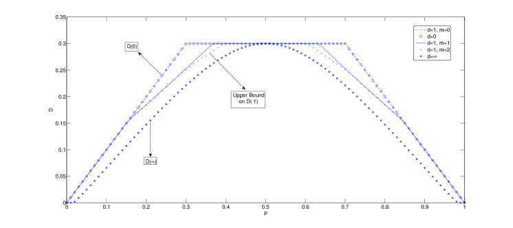
Figure 3: Computing and contrasting $D(d,m)$ and $D(d)$ for a Bernoulli source and binary symmetric channel and Hamming loss. We fix channel cross over probability $\delta=0.3$ and vary source probability in $[0,0.5]$. For $d=1$, we have plotted values for increasing memory, $m=0,1,2$, which yield series of non-trivial non-increasing upper bounds on $D(1)$. $D(0)$ is achieved by symbol symbol by symbol coding, while $D(\infty)=D_{min}$ of Shannon’s joint source channel coding (achieved by separation).

We have run relative value iteration to compute $D(d,m)$ for $d=1$ and some values of $m$, yielding some interesting upper bounds on $D(1)$. Note that the values obtained are exact and do not approximate distortion as the relative value iteration converges in a few iterations. This is because the state space and action space is finite, and it is easy to check that the weak accessibility condition (Definition 4.2.2 [37]) is satisfied. This implies by Proposition 4.3.1 of [37], that relative value iteration converges. Fig. 3 shows the distortion values as a function of source distribution when the cross over probability is fixed, $\delta=0.3$. Fig. 4 shows the distortion values as a function of channel cross over probabilities when the source distribution is fixed, $p=0.3$.

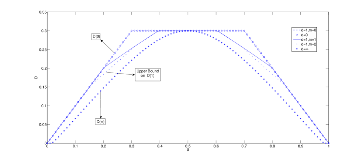
Figure 4: Computing and contrasting $D(d,m)$ and $D(d)$ for a Bernoulli source and binary symmetric channel and Hamming loss. We fix source probability $p=0.3$ and vary the channel cross-over probability in $[0,0.5]$. For $d=1$, we have plotted values for increasing memory, $m=0,1,2$, which yield series of non-trivial non-increasing upper bounds on $D(1)$. $D(0)$ is achieved by symbol symbol by symbol coding, while $D(\infty)=D_{min}$ of Shannon’s joint source channel coding (achieved by separation).

These plots provide insight into the structure of optimal policies in the setting of Section IV, given that we are considering $Bern(p)$ source, $BSC(\delta)$ channel under Hamming loss and $\left|\mathcal{X}\right|=\left|\mathcal{U}\right|=2$. Since $D(1,2)$ is an upper bound on $D(1)$ and hence on $D(d),d\geq 1$, it is clear that for source distributions and channel cross over probabilities where $D(1,2)<D(0)$, symbol by symbol is not optimal. We evaluate this region and show it in Fig. 5. Note when $d=\infty$, since separation is optimal, the region of suboptimality of symbol by symbol is the the complete square $(p\in(0,0.5),\delta\in(0,0.5))$ except the boundary where symbol by symbol is optimal. Also note, as is consistent with the plots, that in the zero lookahead case, we have $D(0)=\min\{p,\delta\}$. Hence, for any lookahead, $d$, for a fixed cross over probability $\delta$, if symbol by symbol encoding-decoding achieves $D(d)$ for $p=p_{0}<0.5$, then it is also optimal for $p\in(p_{0},1-p_{0}]$. Similarly, for a fixed source probability $p$, if symbol by symbol encoding-decoding is optimal for $\delta=\delta_{0}<0.5$, then it is also optimal for $\delta\in(\delta_{0},1-\delta_{0}]$.

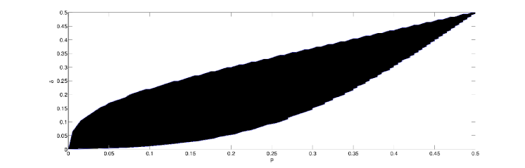
Figure 5: The plot shows a region in the source-channel plane where symbol by symbol coding is suboptimal among schemes with lookahead $d=1$, i.e., it does not achieve $D(1)$. This is the shaded region which is bounded inside by the two curves.

VI Real Time Coding with Limited Lookahead : In the Absence of Feedback

In the previous sections we assumed the availability of perfect unit delay feedback from the decoder to the encoder. We now consider the same setting as that depicted in Fig. 1, but without feedback, and we formulate the problem as a controlled Markov process. Decoders have finite state (see Note 6) and the assumptions A1 and A2 are presumed for similar reasons as in Note 5 in Section V, i.e., memory is finite and decoding is stationary. Here again, we first study the system with modified source, $\{V_{i}\}_{i\in\mathbf{N}}$. The state space for this problem is, $S_{i}=(V_{i},P_{Z_{i}|V^{i}})\in\mathcal{S}$ and the disturbance $W_{i}=V_{i}$. The actions are thus history dependent, $A_{i}=f_{e,i}(S_{0},V^{i-1})=f_{e,i}(S_{0},W^{i-1})$, $S_{0}$ is some fixed initial state with distribution $P_{S}$. Due to Markovity of the source we have,

$$P(W_{i}|W^{i-1},S^{i-1},A^{i}) = K(V_{i-1},V_{i})$$ (103)

$$= P_{W}(W_{i}|S_{i-1},A_{i}).$$ (104)

Denoting $\{P_{Z_{i}|V^{i}}\}_{Z_{i}\in\mathcal{Z}}$ by $\beta_{i}$,

$$\beta_{i}(z) = \frac{P_{V_{i},z|V^{i-1}}}{P_{V_{i}|V_{i-1}}}$$ (105)

$$= \frac{\sum_{Z_{i-1}}P_{Z_{i-1},V_{i},z|V^{i-1}}}{\sum_{Z_{i-1},Z_{i}}P_{Z_{i-1},V_{i},Z_{i}|V^{i-1}}}$$ (106)

$$= \frac{\sum_{Z_{i-1},Y_{i}}P_{Z_{i-1}|V^{i-1}}K(V_{i-1},V_{i})P(Y_{i}|A_{i}(V_{i})){\bf 1}_{\{z=f_{m}(Y_{i},Z_{i-1})\}}}{\sum_{Z_{i-1},Y_{i},Z_{i}}P_{Z_{i-1}|V^{i-1}}K(V_{i-1},V_{i})P(Y_{i}|A_{i}(V_{i})){\bf 1}_{\{Z_{i}=f_{m}(Y_{i},Z_{i-1})\}}}$$ (107)

$$= \frac{\sum_{Z_{i-1},Y_{i}}\beta_{i-1}(Z_{i-1})K(V_{i-1},V_{i})P(Y_{i}|A_{i}(V_{i})){\bf 1}_{\{z=f_{m}(Y_{i},Z_{i-1})\}}}{\sum_{Z_{i-1},Y_{i},Z_{i}}\beta_{i-1}(Z_{i-1})K(V_{i-1},V_{i})P(Y_{i}|A_{i}(V_{i})){\bf 1}_{\{Z_{i}=f_{m}(Y_{i},Z_{i-1})\}}}.$$ (108)

This implies,

$$\beta_{i}=\xi(\beta_{i-1},V_{i},V_{i-1},A_{i})=\xi(S_{i-1},A_{i},W_{i}),\mbox{ }S_{i}=F(S_{i-1},A_{i},W_{i}).$$ (109)

We now have for average cost, with modified cost function $\tilde{\Lambda}(V_{i},\hat{V}_{i})=\Lambda(U_{i},\hat{U}_{i})$ and stationary decoding $\hat{V}^{opt}(\cdot)$,

$$\mathsf{E}\left[\tilde{\Lambda}(V_{i},\hat{V}^{opt}(Y_{i},Z_{i-1}))|V^{i-1},\beta^{i-1},A^{i}\right]$$ (110)

$$= \sum_{\tilde{z}\in\mathcal{Z},\tilde{v}\in\mathcal{V},\tilde{y}\in\mathcal{Y}}P(Z_{i-1}=\tilde{z},V_{i}=\tilde{v},Y_{i}=\tilde{y}|V^{i-1},\beta^{i-1},A^{i})\tilde{\Lambda}(\tilde{v},\hat{V}^{opt}(\tilde{y},\tilde{z})))$$ (111)

$$= \sum_{\tilde{z}\in\mathcal{Z},\tilde{v}\in\mathcal{V},\tilde{y}\in\mathcal{Y}}\beta_{i-1}(\tilde{z})K(V_{i-1},\tilde{v})P(\tilde{y}|A_{i}(\tilde{v}))\tilde{\Lambda}(\tilde{v},\hat{V}^{opt}(\tilde{y},\tilde{z})))$$ (112)

$$= -g(V_{i-1},\beta_{i-1},A_{i})$$ (113)

$$= -g(S_{i-1},A_{i}).$$ (114)

Thus,

$$\frac{1}{n}\sum_{i=1}^{n}\mathsf{E}\left[\tilde{\Lambda}(V_{i},\hat{V}^{opt}(Y_{i},Z_{i-1}))\right]$$ (115)

$$= \frac{1}{n}\sum_{i=1}^{n}\mathsf{E}\left[\mathsf{E}\left[\tilde{\Lambda}(V_{i},\hat{V}^{opt}(Y_{i},Z_{i-1}))|V^{i-1},\beta^{i-1},A^{i}\right]\right]$$ (116)

$$= -\frac{1}{n}\sum_{i=1}^{n}\mathsf{E}\left[g(S_{i-1},A_{i})\right].$$ (117)

We finally write down the ACOE after transforming to the original source (similar to the previous sections),

$$\lambda+h(u_{1},\cdots,u_{d+1},\beta) = \max_{a\in\mathcal{A}}\left[g(u_{1}^{d+1},\beta,a)+\sum_{(\tilde{u},\tilde{y})\in\mathcal{U}\times\mathcal{Y}}P_{U}(\tilde{u})P_{Y|X}(\tilde{y}|a(u_{2},\cdots,u_{d+1},\tilde{u}))h(u_{2}.\cdots,u_{d+1},\tilde{u},\tilde{\beta})\right],$$ (118)

$$\mbox{ }\forall{(u_{1},\cdots,u_{d+1})\in\mathcal{U}^{d+1},}\mbox{ }\beta\in\mathcal{P}(\mathcal{Z}).$$

where

$$g(s,a)=g(u_{1}^{d+1},\beta,a) = -\sum_{\tilde{z}\in\mathcal{Z},\tilde{u}\in\mathcal{U},\tilde{y}\in\mathcal{Y}}\beta(\tilde{z})P_{U}(\tilde{u})P(\tilde{y}|a(u_{2},\cdots,u_{d+1},\tilde{u}))\Lambda(u_{2},\hat{U}^{opt}(\tilde{y},\tilde{z})),$$ (119)

and

$$\tilde{\beta} = \xi((u_{1},\cdots,u_{d+1},\beta),a,(u_{2},\cdots,u_{d+1},\tilde{u}))$$ (120)

$$= \left\{\frac{\sum_{\tilde{z}\in\mathcal{Z},\tilde{y}\in\mathcal{Y}}\beta(\tilde{z})P(\tilde{u})P(\tilde{y}|a(u_{2},\cdots,u_{d+1},\tilde{u})){\bf 1}_{\{z=f_{m}(\tilde{y},\tilde{z})\}}}{\sum_{\tilde{z}\in\mathcal{Z},\tilde{y}\in\mathcal{Y},z\in\mathcal{Z}}\beta(\tilde{z})P(\tilde{u})P(\tilde{y}|a(u_{2},\cdots,u_{d+1},\tilde{u})){\bf 1}_{\{z=f_{m}(\tilde{y},\tilde{z})\}}}\right\}_{z\in\mathcal{Z}}.$$ (121)

Theorem 1 implies that if ACOE Eq. (118) is solved by a real $\lambda^{\ast}$ and a bounded $h(\cdot)$, then $D(d,f_{m},\mathcal{M})=-\lambda^{\ast}$. The results on the structure of optimal policies parallel those outline in Note 4 and hence are omitted.

Note 6

For the setting considered in this section when no feedback is present, we have restricted our attention to finite state decoders only, unlike the previous section where feedback was present and we also considered the case where decoding used complete memory. This is because in the absence of feedback when decoding uses complete memory, the state space is one on the simplex of distributions on alphabets that grows exponentially with the time index and hence the results of the theory presented in Section III are not as directly applicable.

VII Sequential Source Coding with A Side Information “Vending Machine”

In previous sections we considered the problem of real time source-channel communication when the encoder generates channel input symbol sequentially with a lookahead, with or without unit delay noise-free feedback, and the decoder generates the estimate of the source given the channel output and the memory. In this section we consider a rate-distortion problem, where encoding is sequential with lookahead. In addition to it, the decoder can take cost constrained actions, also in a sequential fashion, which affect the quality of the side information correlated with the source symbol it attempts to reconstruct. We consider two classes of such models : one where the encoder has access to the past side information symbols through unit delay noise-free feedback (Section VII-A) and the other when it does not (Section VII-B). The findings of this section are similar in spirit to those of previous sections and assert the universality of the methodology invoked in the paper. We defer the proofs in this section to the Appendix.

Figure 6: The setting of sequential source coding with source lookahead at the encoder and side information vending machine at the decoder. The encoder also knows the past side information symbols through a unit delay noise-free feedback from the decoder.

VII-A Encoder has access to Side Information

The setting depicted in Fig. 6 consists of the following blocks :

• Source Encoder : The encoder has access to source symbols upto a lookahead, $d$ and to the past side information symbols, i.e, $X_{i}=f_{e,i}(U^{i+d},Y^{i-1})$, where $f_{e,i}$ is the encoding function, $f_{e,i}:\mathcal{U}^{i+d}\times\mathcal{Y}^{i-1}\rightarrow\mathcal{X}$, $i\in\mathbf{N}$.

• Memory X : The decoder might not be able to use all of the encoded symbols upto current time due to memory constraints. Memory X is updated as a function of the past state of the memory and the current encoder output, i.e., $M_{i}=f_{m,i}(M_{i-1},X_{i})$, where the $f_{m,i}$ is the memory update function, $f_{m,i}:\mathcal{M}_{i-1}\times\mathcal{X}\rightarrow\mathcal{M}_{i}$, $i\in\mathbf{N}$. Note that the alphabet $\mathcal{M}_{i}$ can grow with $i$, hence this includes the special case of complete memory, i.e., $M_{i}=X^{i}$.

• Actuator : Actuator uses the past Memory X, and the current encoded symbol to generate an action, i.e., $A_{v,i}=f_{v,i}(M_{i-1},X_{i})$, where $f_{v,i}:\mathcal{M}_{i-1}\times\mathcal{X}_{i}\rightarrow\mathcal{A}_{v}$. The action sequence should satisfy the following cost constraint,

  $$\limsup_{N\rightarrow\infty}\mathsf{E}\left[\frac{1}{N}\sum_{i=1}^{N}C(A_{v,i})\right]\leq\Gamma,$$ (122)

  where $C(\cdot)$ is the cost function and $\Gamma$ is the cost constraint.

• Side Information “Vending Machine” : The side information is generated according to $P_{Y|U,A_{v}}$, i.e.,

  $$P(y_{i}|u_{1}^{\infty},x^{i},a_{v}^{i})=P_{Y|U,A_{v}}(y_{i}|u_{i},a_{v,i}).$$ (123)

• Memory Y : The decoder may be limited in its ability to remember all the side information upto current time due to memory constraints. Memory Y is updated as a function of the past state of the memory and the current side information, i.e., $N_{i}=f_{n,i}(N_{i-1},Y_{i})$, where the $f_{n,i}$ is the memory update function, $f_{n,i}:\mathcal{N}_{i-1}\times\mathcal{X}\rightarrow\mathcal{N}_{i}$, $i\in\mathbf{N}$. Here also the alphabet $\mathcal{N}_{i}$ can grow with $i$, hence also includes the special case of complete memory, i.e., $N_{i}=Y^{i}$.

• Source Decoder : Source decoder uses the current encoded symbol, current side information and the past memory states, to construct its estimate of the source symbol, i.e., $\hat{U}_{i}=f_{d,i}(X_{i},Y_{i},M_{i-1},N_{i-1})$, the decoding rule is the map, $f_{d,i}:\mathcal{X}\times\mathcal{Y}\times\mathcal{M}_{i-1}\times\mathcal{N}_{i-1}\rightarrow\hat{\mathcal{U}}$. The complete memory case corresponds to the decoding, $\hat{U}_{i}(X^{i},Y^{i})$.

The alphabets $\mathcal{U},\mathcal{X},\mathcal{A}_{v},\mathcal{Y},\mathcal{M},\mathcal{N}$ are assumed to be finite. Note that the finiteness of the alphabets implies we may assume, without loss of generality, that $0\leq\Lambda(\cdot)\leq\Lambda_{max}<\infty$ and $0\leq C(\cdot)\leq\Gamma_{max}<\infty$. We make the further assumption that there exists $a\in\mathcal{A}_{v}$ such that $C(a)=0$. Thus it makes sense to consider cost constraints, $\Gamma\in[0,\Gamma_{max}]$.

Our approach to construction of the ACOE is similar to that taken in previous sections, we first consider the system with modified source, $\{V_{i}=U_{i}^{i+d}\}_{i\in\mathbf{N}}$ and it is equivalent to consider source and action encoding rules as mappings, $\{f_{e,i}(v,V^{i-1},Y^{i-1})\}_{v\in\mathcal{V}}$ and $\{f_{v,i}(x,X^{i-1})\}_{x\in\mathcal{X}}$. Hence the modified vending machine is,

$$P(Y_{i}|V_{i},A_{v,i}(X_{i}))=P(Y_{i}|U_{i},A_{v,i}(X_{i})),$$ (124)

and the modified cost function is,

$$\tilde{\Lambda}(V_{i},\hat{V}_{i})=\Lambda(U_{i},\hat{U}_{i}).$$ (125)

We study two scenarios under this setting :

VII-A1 Complete Memory

Here $M_{i}=X^{i}$ and $N_{i}=Y^{i}$. Note that we can restrict our attention to optimal decoders of the form, $\hat{U}_{i}(X^{i},Y^{i})=\hat{U}_{Bayes}(X^{i},Y^{i})$ (cf. Lemma 3). Let us denote the minimum expected average distortion achieved to be $D^{FB}_{a}(d)$. Here $FB$ superscript indicating we have side information available as a feedback to the encoder, $a$ subscript denotes presence of actions and $d$ stands for lookahead. We have the average cost optimality equation as,

$$\rho^{\lambda}(u_{1},\cdots,u_{d+1},\beta)+h^{\lambda}(u_{1},\cdots,u_{d+1},\beta)$$ (126)

$$= \max_{(a_{e},a_{v})}\left[g^{\lambda}(u_{1},\cdots,u_{d+1},\beta,a_{e},a_{v})+\sum_{\tilde{u}\in\mathcal{U},\tilde{x}\in\mathcal{X},\tilde{y}\in\mathcal{Y}}P(\tilde{u}){\bf 1}_{\{\tilde{x}=a_{e}(u_{2},\cdots,u_{d+1},\tilde{u})\}}P(\tilde{y}|u_{2},a_{v}(\tilde{x}))h(u_{d},\cdots,u_{d+1},\tilde{u},\tilde{\beta})\right]$$

$$\mbox{ }\forall\mbox{ }(u_{1},\cdots,u_{d+1})\in\mathcal{U}^{d+1},\beta\in\mathcal{P}(\mathcal{U}^{d+1}),$$

where $(a_{e},a_{v})\in\mathcal{A}_{e}\times\mathcal{A}_{v}$ and $\tilde{\beta}=G(\beta,a_{e},a_{v},(u_{2}^{d+1},\tilde{u},\tilde{x},\tilde{y}))$ (cf. Appendix B) is the updated belief and $g^{\lambda}(\cdot)$ is the Lagrangian augmented cost,

$$g^{\lambda}(u_{1},\cdots,u_{d+1},\beta,a_{e},a_{v})$$ (127)

$$= g(u_{1},\cdots,u_{d+1},\beta,a_{e},a_{v})+\lambda\left(\Gamma-l(u_{1},\cdots,u_{d+1},\beta,a_{e},a_{v})\right)$$

$$= -\min_{\hat{u}\in\mathcal{U}}\sum_{\overline{u}\in\mathcal{U}}\beta_{1}(\overline{u})\Lambda(\overline{u},\hat{u})+\lambda\left(\Gamma-\sum_{\tilde{u}\in\mathcal{U},\tilde{x}\in\mathcal{X}}P(\tilde{u}){\bf 1}_{\{\tilde{x}=a_{e}(u_{2},\cdots,u_{d+1},\tilde{u})\}}C(A_{v}(\tilde{x}))\right).$$ (128)

We have now the following theorem, with proof in Appendix B.

Theorem 10

For a fixed lookahead, $d$, let $(\rho^{\lambda}(\cdot),h^{\lambda}(\cdot))$ solves the ACOE Eq. (126). Then the optimal average distortion is given by,

$$D^{FB}_{a}(d)=-\inf_{\lambda\geq 0}\sup_{x\in\mathcal{U}^{d+1}\times\mathcal{P}(\mathcal{U}^{d+1})}\rho^{\lambda}(x).$$ (129)

Note 7

Note that for a fixed finite lookahead, $d\geq 1$, $D^{FB}_{a}(d)$ contrasts the minimum distortion at, $d=0$, where symbol by symbol encoding, action-encoding and decoding are optimal, i.e,

$$D^{FB}_{a}(0)=\min_{X:\mathcal{U}\rightarrow\mathcal{X},A:\mathcal{X}\rightarrow\mathcal{A}}\mathsf{E}\left[\Lambda\left(U,\hat{U}_{Bayes}(P_{U|X,Y})\right)\right],$$ (130)

while at infinite lookahead, $d=\infty$, the minimum distortion is given by the distortion rate function at unit rate by results from [22], i.e,

$$D^{FB}_{a}(\infty) = \min_{P_{A_{v},W|U},\hat{U}^{opt}:\mathcal{W}\times\mathcal{Y}\rightarrow\hat{\mathcal{U}}}\mathsf{E}\left[\Lambda\left(U,\hat{U}^{opt}(W,Y)\right)\right]$$

such that $$I(U;W,A_{v})\leq\log_{2}\left|\mathcal{X}\right|$$ (131)

$$\left|\mathcal{W}\right|\leq\left|\mathcal{U}\right|\left|\mathcal{A}_{v}\right|+2$$

$$\mathsf{E}\left[C(A_{v})\right]\leq\Gamma,$$

where $I(\cdot;\cdot)$ is the mutual information (cf. [38]). The above distortion is basically the distortion rate function (cf. Theorem 3 [22]) evaluated at the rate equal to the cardinality of the alphabet $\left|\mathcal{X}\right|$. The proofs for Equations (130) and (131) are similar to those of Lemma 5 and Lemma 9.

VII-A2 Finite Memory

In this section, all memories are finite (not growing with time). With the object of minimizing the expected distortion, we cast this problem as a constrained Markov decision process. To be able to do that, for reasons discussed in Section V, we assume, $f_{m,i}=f_{m}$, $f_{n,i}=f_{n}$, $\mathcal{M}_{i}=\mathcal{M}$ and $\mathcal{N}_{i}=\mathcal{N}$ for all $i\in\mathbf{N}$, the alphabets $\mathcal{M}$, $\mathcal{N}$ being finite. We further assume stationary optimal decoding and actuator policies, i.e., $f_{d,i}(\cdot,\cdot,\cdot,\cdot)=U^{opt}(\cdot,\cdot,\cdot,\cdot)$, and $f_{a,i}(\cdot,\cdot)=A_{v}^{opt}(\cdot,\cdot)$ for all $i\in\mathbf{N}$.
Fix a lookahead $d$. Now for fixed $\lambda\geq 0$, the average cost optimality equation is,

$$\rho^{\lambda}(u_{1},\cdots,u_{d+1},m,n)+h^{\lambda}(u_{1},\cdots,u_{d+1},m,n)$$ (132)

$$= \max_{a\in\mathcal{A}}\left[g^{\lambda}(u_{1},\cdots,u_{d+1},m,n,a)+\sum_{\tilde{u}\in\mathcal{U},\tilde{x}\in\mathcal{X},\tilde{y}\in\mathcal{Y}}P(\tilde{u}){\bf 1}_{\{\tilde{x}=a(u_{2},\cdots,u_{d+1},\tilde{u})\}}P(\tilde{y}|u_{2},A^{opt}_{v}(\tilde{x}))h(u_{d},\cdots,u_{d+1},\tilde{u},\tilde{m},\tilde{n}))\right]$$

$$\mbox{ }\forall\mbox{ }(u_{1},\cdots,u_{d+1})\in\mathcal{U}^{d+1},m\in\mathcal{M},n\in\mathcal{N},$$

where $\tilde{m}=f_{m}(m,\tilde{x})$ and $\tilde{n}=f_{n}(n,\tilde{y})$ are memory updates and $g^{\lambda}(\cdot)$ is the Lagrangian augmented cost,

$$g^{\lambda}(u_{1},\cdots,u_{d+1},m,n,a)$$

$$= g(u_{1},\cdots,u_{d+1},m,n,a)+\lambda\left(\Gamma-l(u_{1},\cdots,u_{d+1},m,n,a)\right)$$

$$= -\sum_{\tilde{u}\in\mathcal{U},\tilde{x}\in\mathcal{X},\tilde{y}\in\mathcal{Y}}P(\tilde{u}){\bf 1}_{\{\tilde{x}=a(u_{2},\cdots,u_{d+1},\tilde{u})\}}P(\tilde{y}|u_{2},A^{opt}_{v}(\tilde{x}))\Lambda(u_{2},\hat{U}_{Bayes}(\tilde{x},\tilde{y},m,n))$$

$$+ \lambda\left(\Gamma-\sum_{\tilde{u}\in\mathcal{U},\tilde{x}\in\mathcal{X}}P(\tilde{u}){\bf 1}_{\{\tilde{x}=a_{e}(u_{2},\cdots,u_{d+1},\tilde{u})\}}C(A_{v}^{opt}(\tilde{x}))\right).$$ (134)

Let us denote the optimal distortion by $D^{FB}_{a}(d,\mathcal{M},\mathcal{N})$. We have now the following theorem, with proof in Appendix C.

Theorem 11

For a fixed lookahead, $d$, let $(\rho^{\lambda}(\cdot),h^{\lambda}(\cdot))$ solves the ACOE Eq. (132). Then the optimal average distortion is given by,

$$D^{FB}_{a}(d,\mathcal{M},\mathcal{N})=-\inf_{\lambda\geq 0}\sup_{x\in\mathcal{U}^{d+1}\times\mathcal{M}\times\mathcal{N}}\rho^{\lambda}(x).$$ (135)

VII-B Encoder does not have access to Side Information

Here encoder does not recieve any knowledge about side information. In this section also, we make assumptions A1 and A2 and further assume finite state decoders (for reasons similar to those outlined in Note 6). For a fixed lookahead $d$, $\lambda\geq 0$, we have the average cost optimality equation,

$$\rho^{\lambda}(u_{1},\cdots,u_{d+1},\beta,\gamma)+h^{\lambda}(u_{1},\cdots,u_{d+1},\beta,\gamma)$$ (136)

$$= \max_{a\in\mathcal{A}}\left[g^{\lambda}(u_{1},\cdots,u_{d+1},\beta,\gamma,a)+\sum_{\tilde{u}\in\mathcal{U},\tilde{x}\in\mathcal{X},\tilde{y}\in\mathcal{Y}}P(\tilde{u}){\bf 1}_{\{\tilde{x}=a(u_{2},\cdots,u_{d+1},\tilde{u})\}}P(\tilde{y}|u_{2},A^{opt}_{v}(\tilde{x}))h(u_{d},\cdots,u_{d+1},\tilde{u},\tilde{\beta},\tilde{\gamma}))\right]$$

$$\mbox{ }\forall\mbox{ }(u_{1},\cdots,u_{d+1})\in\mathcal{U}^{d+1},\beta\in\mathcal{P}(\mathcal{M}),\gamma\in\mathcal{P}(\mathcal{N}),$$

where $\tilde{\beta}=\xi_{m}(\beta,u_{1}^{d+1},\tilde{u},a)$ and $\tilde{\gamma}=\xi_{n}(\gamma,u_{1}^{d+1},\tilde{u},a)$ are belief updates (cf. Appendix D) and $g^{\lambda}(\cdot)$ is the Lagrangian augmented cost,

$$g^{\lambda}(u_{1},\cdots,u_{d+1},\beta,\gamma,a)$$

$$= g(u_{1},\cdots,u_{d+1},\beta,\gamma,a)+\lambda\left(\Gamma-l(u_{1},\cdots,u_{d+1},\beta,\gamma,a)\right)$$

$$= -\sum_{\tilde{m}\in\mathcal{M},\tilde{n}\in\mathcal{N},\tilde{u}\in\mathcal{U},\tilde{x}\in\mathcal{X},\tilde{y}\in\mathcal{Y}}\beta(\tilde{m})\gamma(\tilde{n})P(\tilde{u}){\bf 1}_{\{\tilde{x}=a(u_{2},\cdots,u_{d+1},\tilde{u})\}}P(\tilde{y}|u_{2},A^{opt}_{v}(\tilde{x}))\Lambda(u_{2},\hat{U}_{Bayes}(\tilde{x},\tilde{y},\tilde{m},\tilde{n}))$$

$$+ \lambda\left(\Gamma-\sum_{\tilde{u}\in\mathcal{U},\tilde{x}\in\mathcal{X}}P(\tilde{u}){\bf 1}_{\{\tilde{x}=a_{e}(u_{2},\cdots,u_{d+1},\tilde{u})\}}C(A_{v}^{opt}(\tilde{x}))\right).$$ (138)

Let us denote the optimal distortion by $D^{NF}_{a}(d,\mathcal{M},\mathcal{N})$ (NF standing for no feedback of side information symbols). We can now state the following theorem whose proof is defered to Appendix D.

Theorem 12

For a fixed lookahead, $d$, suppose that $(\rho^{\lambda}(\cdot),h^{\lambda}(\cdot))$ solves the ACOE Eq. (136). Then the optimal average distortion is given by,

$$D^{NF}_{a}(d,\mathcal{M},\mathcal{N})=-\inf_{\lambda\geq 0}\sup_{x\in\mathcal{U}^{d+1}\times\mathcal{P}(\mathcal{M})\times\mathcal{P}(\mathcal{N})}\rho^{\lambda}(x).$$ (139)

Note 8

Note that the ACOE in this section on sequential source coding with lookahead and a side information vending machine is amenable to computational solutions as in Section V-B. Here also $D^{FB}_{a}(d,\mathcal{M},\mathcal{N})$ can be computed for increasing memories exactly, and yield non trivial bounds on $D^{FB}_{a}(d)$.

VIII Summary of the Results

In this section we provide a summary of the various settings considered in this paper on real time communication with fixed finite lookahead at the encoder, and the transformations performed to cast the problem as (constrained or unconstrained) Markov decision process. The methodology is to construct an average cost optimality equation (ACOE), and seek its solution. We have considered two classes of problems in this paper :

1. Real Time Communication, Fig. 1. The problem is characterized by tuple $(\mathcal{S},\mathcal{A},\mathcal{W},F,P_{S},P_{W},g)$, the meaning of various symbols being explained in Section III. The general ACOE is,

   $$\lambda(s)+h(s)=\max_{a\in\mathcal{A}}\left[g(s,a)+\sum_{w\in\mathcal{W}}P_{W}(w|s,a)h(F(s,a,w))\right]\mbox{ }\forall\mbox{ }s\in\mathcal{S}.$$ (140)

   Note in all the settings we considered, $\sup$ is replaced by $\max$ as the set of actions is finite. If $\exists\ \lambda^{\ast}\in\mathbf{R}$ and a bounded $h(\cdot)$, satisfying the above equation, then using Theorem 1, the minimum distortion is $-\lambda^{\ast}$. The following table exhibits the transformations, along with pointers to the equations in the paper that cast the problem of Fig. 1 as an unconstrained Markov decision process :
   

   Real-Time Communication, Fig. 1, Lookahead, $d$	Noise-Free Feedback, Complete Memory Decoding	Noise-free Feedback, Finite Memory ($\mathcal{M}$) Decoder	No Feedback, Finite Memory ($\mathcal{M}$) Decoder
   $\mathcal{S}$, state space	$\mathcal{U}^{d+1}\times\mathcal{P}(\mathcal{U}^{d+1})$	$\mathcal{U}^{d+1}\times\mathcal{M}$	$\mathcal{U}^{d+1}\times\mathcal{P}(\mathcal{M})$
   $\mathcal{A}$, action space	$\mbox{Mappings}:\mathcal{U}^{d+1}\rightarrow\mathcal{X}$	$\mbox{Mappings}:\mathcal{U}^{d+1}\rightarrow\mathcal{X}$	$\mbox{Mappings}:\mathcal{U}^{d+1}\rightarrow\mathcal{X}$
   $\mathcal{W}$, disturbance	$\mathcal{U}^{d+1}\times\mathcal{Y}$	$\mathcal{U}^{d+1}\times\mathcal{Y}$	$\mathcal{U}^{d+1}$
   $F(\cdot)$	Eq. (39)	Eq. (88)	Eq. (109)
   $P_{W}(\cdot|S,A)$	Eq. (29)	Eq. (87)	Eq. (104)
   $g(S,A)$, reward	Eq. (52)	Eq. (101)	Eq. (119)
   ACOE	Eq. (53)	Eq. (102)	Eq. (118)

   
   

2. Source Coding with a Side Information Vending Machine, Fig. 6 : The problem is characterized by tuple $(\mathcal{S},\mathcal{A},\mathcal{W},F,P_{s},P_{w},g,l,\Gamma)$ explained in Section III-A. Here also the general ACOE is,

   $$\rho^{\lambda}(s)+h^{\lambda}(s)=\sup_{a\in\mathcal{A}}\left[g^{\lambda}(s,a)+\sum_{w\in\mathcal{W}}P(w|s,a)h(F(s,a,w))\right]\mbox{ }\forall\mbox{ }s\in\mathcal{S},$$ (141)

   where $\lambda$ is the Lagrangian parameter. Minimum distortion is given by the Theorems 10, 11 and 12, respectively, for the cases tabulated below.
   

   Source Coding With SI “Vendor”, Fig. 6, Lookahead, $d$	Noise-Free Feedback, Complete Memory Decoding	Noise-free Feedback, Finite Memory ($\mathcal{M},\mathcal{N}$) Decoder	No Feedback, Finite Memory ($\mathcal{M},\mathcal{N}$) Decoder
   $\mathcal{S}$, state space	$\mathcal{U}^{d+1}\times\mathcal{P}(\mathcal{U}^{d+1})$	$\mathcal{U}^{d+1}\times\mathcal{M}\times\mathcal{N}$	$\mathcal{U}^{d+1}\times\mathcal{P}(\mathcal{M})\times\mathcal{P}(\mathcal{N})$
   $\mathcal{A}$, action space	$\mbox{Mappings}:\mathcal{U}^{d+1}\times\mathcal{X}\rightarrow\mathcal{X}\times\mathcal{A}_{v}$	$\mbox{Mappings}:\mathcal{U}^{d+1}\rightarrow\mathcal{X}$	$\mbox{Mappings}:\mathcal{U}^{d+1}\rightarrow\mathcal{X}$
   $\mathcal{W}$, disturbance	$\mathcal{U}^{d+1}\times\mathcal{X}\times\mathcal{Y}$	$\mathcal{U}^{d+1}\times\mathcal{X}\times\mathcal{Y}$	$\mathcal{U}^{d+1}$
   $F(\cdot)$	Eq. (166) (Appendix B)	Eq. (181) (Appendix C)	Eq. (199) (Appendix D)
   $P_{w}(\cdot|S,A)$	Eq. (162) (Appendix B)	Eq. (180) (Appendix C)	Eq. (194) (Appendix D)
   $g^{\lambda}(S,A)$, Lagrangian augmented reward	Eq. (173) (Appendix B)	Eq. (190) (Appendix C)	Eq. (208) (Appendix D)
   ACOE	Eq. (126)	Eq. (132)	Eq. (136)

IX Conclusion

In this paper, we consider an important class of problems in real time coding : a memoryless source is to be communicated over a memoryless channel, with sequential encoding and decoding and with a fixed finite lookahead of future symbols available at the encoder. Unit delay feedback may or may not be present, and decoding is based on the channel output symbols without delay, with or without a memory constraint. In all these scenarios, under the objective of minimizing the per-symbol distortion, we obtain average cost optimality equations whose solution yields the minimum achievable distortion, as well as sufficient conditions for the optimality of stationary policies. We contrast the minimum distortion at a fixed lookahead, with the best achievable with zero lookahead, where symbol by symbol encoding-decoding is optimal, and with the infinite lookahead case, for which the minimum achievable per symbol distortion is shown to coincide with that for the classical joint source channel coding problem, where separation is optimal. For the Bernoulli source and binary symmetric channel under Hamming loss, in case of finite state decoders, we compute exactly the minimum distortion values for various memory sizes, and study the upper bounds that they yield on the minimum distortion for a fixed lookahead in the absence of memory constraints. Answering the question “to look or not to lookahead”, we characterize general conditions on the source and channel such that symbol by symbol encoding-decoding is optimal within the class of schemes of a given lookahead. We obtain and plot the region for source and channel parameters in case of Bernoulli source, binary symmetric channel and Hamming distortion, where the symbol by symbol policy is strictly suboptimal. We then demonstrate that this framework of casting real time coding problems as Markov decision problems with average cost criteria can be useful in various other frameworks by applying this same methodology in source coding problem with a side information vending machine, where encoder encodes the source sequentially, with a possible lookahead, decoder takes cost constrained actions to receive the side information about the source. This setting is cast as a constrained Markov decision problem and it is shown that a stationary randomized policy can attain the minimum per-symbol distortion which is characterized as the solution to a saddle point equation.

Appendix A

In Section II the minimum expected distortion is defined as,

$$D(d)=\inf_{\{f_{e},f_{m},f_{d}\}}\limsup_{N\rightarrow\infty}\mathsf{E}\left[\frac{1}{N}\sum_{i=1}^{N}\Lambda(U_{i},\hat{U}_{i})\right].$$ (142)

Note that $\inf$ in the above definition can be replaced by $\min$ over the class of $(f_{e},f_{m},f_{d})$-policies as outlined in Section II. This is argued by constructing an $(f_{e},f_{m},f_{d})$-policy that achieves $D(d)$. Fix lookahead $d$. As $D(d)$ always exists (also it is finite due to our assumption that $\Lambda(\cdot,\cdot)\leq\Lambda_{max}<\infty$), for a positive non-increasing vanishing sequence $\{\epsilon_{m}\}_{m\geq 1}$, we can construct a sequence of policies, i.e., $\{\mu_{m}\}_{m\geq 1}$ with expected average distortion $D_{\mu_{m}}(d)$, i.e.,

$$D_{\mu_{m}}(d) = \limsup_{N\rightarrow\infty}\mathsf{E}_{\mu_{m}}\left[\frac{1}{N}\sum_{i=1}^{N}\Lambda(U_{i},\hat{U}_{i})\right]$$ (143)

$$= \limsup_{N\rightarrow\infty}D^{N}_{\mu_{m}}(d),$$ (144)

($\mathsf{E}_{\mu_{m}}$ is the expectation with respect to the joint probability distribution induced when the policy used is $\mu_{m}$), such that $D_{\mu_{m}}(d)$ is a monotone non-increasing sequence converging to $D(d)$. By the definition of $\limsup$, for every $m\geq 1$, $\exists\ N_{m}(\epsilon_{m})$ such that $\forall\ N\geq N_{m}$ ($N_{m}$ being function of $\epsilon_{m}$ is implied henceforth),

$$D^{N}_{\mu_{m}}(d)\leq D_{\mu_{m}}(d)+\epsilon_{m}.$$ (145)

Now define a block-length sequence $\{l_{m}\in\mathbf{N}\}_{m\geq 1}$, satisfying the following requirements,

• R1 : $l_{m}>\sum_{i=1}^{m-1}l_{i}$ and that $\frac{\sum_{i=1}^{m-1}l_{i}}{l_{m}}\rightarrow 0$ as $m\rightarrow\infty$.

• R2 : $l_{m}>\max\{N_{m},N_{m+1}\}$ and that $\frac{\max\{N_{m},N_{m+1}\}}{l_{m}}\rightarrow 0$ as $m\rightarrow\infty$.

Note that we can always choose such a sequence, for eg. $l_{m}=\max\{N_{m},N_{m+1}\}(\sum_{i=1}^{m-1}l_{i})$. We define a block-coding scheme $\mu^{\ast}$ which operates with block length $l_{i}$ in $i^{th}$ block with scheme $\mu_{i}$. Operating this scheme for time $N\in(\sum_{i=1}^{m}l_{i},\sum_{i=1}^{m+1}l_{i}]$ for some $m=m(N)$, (note $m(N)\rightarrow\infty$ as $N\rightarrow\infty$) we can bound the normalized distortion as:

• (Case 1) $N-\sum_{i=1}^{m}l_{i}<N_{m+1}$

  $$D^{N}_{\mu^{\ast}}(d) \stackrel{{\scriptstyle(a)}}{{\leq}} \left(\frac{\sum_{i=1}^{m-1}l_{i}}{N}\right)\Lambda_{max}+\frac{l_{m}}{N}\left(D_{\mu_{m}}(d)+\epsilon_{m}\right)+\left(\frac{N-\sum_{i=1}^{m}l_{i}}{N}\right)\Lambda_{max}$$ (146)

  $$= \left(\frac{N-l_{m}}{N}\right)\Lambda_{max}+\frac{l_{m}}{N}\left(D_{\mu_{m}}(d)+\epsilon_{m}\right)$$ (147)

  $$\leq \left(\frac{\sum_{i=1}^{m-1}l_{i}+N_{m+1}}{l_{m}}\right)\Lambda_{max}+D_{\mu_{m}}(d)+\epsilon_{m},$$ (148)

  where (a) is due to the fact that $l_{m}>N_{m}$ (requirement R2) and hence distortion in block $m$ is bounded above by $D_{\mu_{m}}(d)+\epsilon_{m}$.

• (Case 2) $N-\sum_{i=1}^{m}l_{i}\geq N_{m+1}$

  $$D^{N}_{\mu^{\ast}}(d) \stackrel{{\scriptstyle(b)}}{{\leq}} \left(\frac{\sum_{i=1}^{m-1}l_{i}}{N}\right)\Lambda_{max}+\frac{l_{m}}{N}\left(D_{\mu_{m}}(d)+\epsilon_{m}\right)+\left(\frac{N-\sum_{i=1}^{m}l_{i}}{N}\right)\left(D_{\mu_{m+1}}(d)+\epsilon_{m+1}\right)$$ (149)

  $$\stackrel{{\scriptstyle(c)}}{{\leq}} \left(\frac{\sum_{i=1}^{m-1}l_{i}}{N}\right)\Lambda_{max}+\frac{l_{m}}{N}\left(D_{\mu_{m}}(d)+\epsilon_{m}\right)+\left(\frac{N-l_{m}}{N}\right)\left(D_{\mu_{m}}(d)+\epsilon_{m}\right)$$ (150)

  $$= \left(\frac{\sum_{i=1}^{m-1}l_{i}}{N}\right)\Lambda_{max}+D_{\mu_{m}}(d)+\epsilon_{m}$$ (151)

  $$\leq \left(\frac{\sum_{i=1}^{m-1}l_{i}+N_{m+1}}{l_{m}}\right)\Lambda_{max}+D_{\mu_{m}}(d)+\epsilon_{m},$$ (152)

  where (b) follows from bounding the distortion in block $m$ as in (a) and similarly as $N-\sum_{i=1}^{m}l_{i}\geq N_{m+1}$, bounding distortion in block $m+1$ by $D_{\mu_{m+1}}(d)+\epsilon_{m+1}$ and (c) follows from the fact that both $D_{\mu_{m}}(d)$ and $\epsilon_{m}$ are non-increasing sequences.

Thus we see in both the above cases, for any time $N$, the normalized distortion is bounded above as,

$$D^{N}_{\mu^{\ast}}(d) \leq \left(\frac{\sum_{i=1}^{m-1}l_{i}+N_{m+1}}{l_{m}}\right)\Lambda_{max}+D_{\mu_{m}}(d)+\epsilon_{m},$$ (153)

which implies that the expected average distortion under policy $\mu^{\ast}$ is,

$$D_{\mu^{\ast}}(d) \leq \limsup_{N\rightarrow\infty}\left[\left(\frac{\sum_{i=1}^{m-1}l_{i}+N_{m+1}}{l_{m}}\right)\Lambda_{max}+D_{\mu_{m}}(d)+\epsilon_{m}\right]$$ (154)

$$\leq \limsup_{N\rightarrow\infty}\left(\frac{\sum_{i=1}^{m-1}l_{i}}{l_{m}}\right)\Lambda_{max}+\limsup_{N\rightarrow\infty}\left(\frac{N_{m+1}}{l_{m}}\right)\Lambda_{max}+\limsup_{N\rightarrow\infty}\left(D_{\mu_{m}}(d)+\epsilon_{m}\right)$$ (155)

$$\stackrel{{\scriptstyle(d)}}{{=}} D(d),$$ (156)

where (d) follows from the fact that $\frac{\sum_{i=1}^{m-1}l_{i}}{l_{m}}\rightarrow 0$ and $\frac{N_{m+1}}{l_{m}}\rightarrow 0$ by requirements R1 and R2 respectively, since $m(N)\rightarrow\infty$ as $N\rightarrow\infty$. Thus we have a scheme $\mu^{\ast}$ with minimum expected distortion $D_{\mu^{\ast}}(d)\leq D(d)$, but we know for any scheme $\mu^{\ast}$, $D(d)\leq D_{\mu^{\ast}}(d)$, implying $D_{\mu^{\ast}}(d)=D(d)$.

Appendix B Proof of Theorem 10

We will first obtain the ACOE Eq. (126). Define the state sequence, $S_{i}=(V_{i},\{P_{V_{i}=v|X^{i},Y^{i}}\}_{v\in\mathcal{V}})$, disturbance sequence, $W_{i}=(V_{i},X_{i},Y_{i})$, action sequence, $A_{i}=\{f_{e,i}(v,V^{i-1},Y^{i-1}),f_{v,i}(x,X^{i-1})\}_{v\in\mathcal{V},x\in\mathcal{X}}$ is clearly a history dependent action, i.e. function of $W^{i-1}=(V^{i-1},X^{i-1},Y^{i-1})$. We will now verify the conditions for the defined state sequence, disturbance and action sequence to form a controlled markov process. With some abuse of notation, we denote,

$$\beta_{i} = \{P_{V_{i}=v|X^{i},Y^{i}}\}_{v\in\mathcal{V}}$$ (157)

$$A_{e,i} = f_{e,i}(\cdot,V^{i-1},Y^{i-1})$$ (158)

$$A_{v,i} = f_{v,i}(\cdot,X^{i-1}).$$ (159)

Now,

$$P(W_{i}|W^{i-1},S^{i-1},A^{i}) = P(V_{i},X_{i},Y_{i}|V^{i-1},X^{i-1},Y^{i-1},A_{v}^{i},A_{e}^{i},\beta^{i})$$ (160)

$$= K(V_{i-1},V_{i}){\bf 1}_{\{X_{i}=A_{e,i}(V_{i})\}}P(Y_{i}|V_{i},A_{v,i}(X_{i}))$$ (161)

$$= P_{W}(W_{i}|S_{i-1},A_{i})$$ (162)

$$\beta_{i} = \left\{\frac{\sum_{V_{i-1}}\beta_{i-1}(V_{i-1})K(V_{i-1},v){\bf 1}_{\{X_{i}=A_{e,i}(v)\}}P(Y_{i}|v,A_{v,i}(X_{i}))}{\sum_{V_{i-1},V_{i}}\beta_{i-1}(V_{i-1})K(V_{i-1},V_{i}){\bf 1}_{\{X_{i}=A_{e,i}(V_{i})\}}P(Y_{i}|V_{i},A_{v,i}(X_{i}))}\right\}_{v\in\mathcal{V}}$$ (163)

$$= G(\beta_{i-1},A_{e,i},A_{v,i},V_{i},X_{i},Y_{i})$$ (164)

$$= G(\beta_{i-1},A_{i},W_{i}),$$ (165)

which implies,

$$S_{i}=F(S_{i-1},A_{i},W_{i}).$$ (166)

The optimal decoding is $\hat{V}_{Bayes}(P_{V_{i}|X^{i},Y^{i}})$. Also let $g(S_{i},A_{i+1})=-\mathsf{E}\left[\tilde{\Lambda}(V_{i},\hat{V}_{Bayes}(P_{V_{i}|X^{i},Y^{i}}))\Big{|}Y^{i}\right]$ so that we have

$$\inf\limsup_{N\rightarrow\infty}\mathsf{E}\left[\frac{1}{N}\sum_{i=1}^{N}\tilde{\Lambda}(V_{i},\hat{V}_{Bayes}(X^{i},Y^{i})\right] = -\sup\liminf_{N\rightarrow\infty}\mathsf{E}\left[\frac{1}{N}\sum_{i=1}^{N}g(S_{i-1},A_{i})\right].$$ (167)

Also for the cost constraint on action,

$$\mathsf{E}\left[{C}(A_{v,i}(X_{i}))\Big{|}V^{i-1},X^{i-1},Y^{i-1},A^{i}\right] = \sum_{\tilde{v}\in\mathcal{V},\tilde{x}\in\mathcal{X}}K(V_{i-1},\tilde{v}){\bf 1}_{\{\tilde{x}=A_{e,i}(\tilde{v})\}}{C}(A_{v,i}(\tilde{x}))$$ (168)

$$= l(S_{i-1},A_{i}),$$ (169)

which imply,

$$\limsup_{N\rightarrow\infty}\mathsf{E}\left[\frac{1}{N}\sum_{i=1}^{N}C(A_{v,i})\right]=\limsup_{N\rightarrow\infty}\mathsf{E}\left[\frac{1}{N}\sum_{i=1}^{N}l(S_{i-1},A_{i})\right].$$ (170)

Thus the problem of minimizing the average distortion subject to constraints on the vending action is equivalent to a constrained Markov decision process, $(\mathcal{S},\mathcal{A},\mathcal{W},F,P_{S},P_{W},g,l,\Gamma)$ (note here the number of constraints is $k=1$). Fix a lookahead $d$. Let $\beta_{1}$ denote the marginal of belief $\beta$ with respect to the first argument. Now for fixed $\lambda\geq 0$, we have the average cost optimality equation as,

$$\rho^{\lambda}(u_{1},\cdots,u_{d+1},\beta)+h^{\lambda}(u_{1},\cdots,u_{d+1},\beta)$$ (171)

$$= \max_{(a_{e},a_{v})}\left[g^{\lambda}(u_{1},\cdots,u_{d+1},\beta,a_{e},a_{v})+\sum_{\tilde{u}\in\mathcal{U},\tilde{x}\in\mathcal{X},\tilde{y}\in\mathcal{Y}}P(\tilde{u}){\bf 1}_{\{\tilde{x}=a_{e}(u_{2},\cdots,u_{d+1},\tilde{u})\}}P(\tilde{y}|u_{2},a_{v}(\tilde{x}))h(u_{d},\cdots,u_{d+1},\tilde{u},\tilde{\beta})\right]$$

$$\mbox{ }\forall\mbox{ }(u_{1},\cdots,u_{d+1})\in\mathcal{U}^{d+1},\beta\in\mathcal{P}(\mathcal{U}^{d+1}),$$

where $\tilde{\beta}=G(\beta,a_{e},a_{v},(u_{2}^{d+1},\tilde{u},\tilde{x},\tilde{y}))$ is the updated belief, $(a_{e},a_{v})\in\mathcal{A}_{e}\times\mathcal{A}_{v}$ and $g^{\lambda}(\cdot)$ is the Lagrangian augmented cost,

$$g^{\lambda}(u_{1},\cdots,u_{d+1},\beta,a_{e},a_{v})$$ (172)

$$= g(u_{1},\cdots,u_{d+1},\beta,a_{e},a_{v})+\lambda\left(\Gamma-l(u_{1},\cdots,u_{d+1},\beta,a_{e},a_{v})\right)$$

$$= -\min_{\hat{u}\in\mathcal{U}}\sum_{\overline{u}\in\mathcal{U}}\beta_{1}(\overline{u})\Lambda(\overline{u},\hat{u})+\lambda\left(\Gamma-\sum_{\tilde{u}\in\mathcal{U},\tilde{x}\in\mathcal{X}}P(\tilde{u}){\bf 1}_{\{\tilde{x}=a_{e}(u_{2},\cdots,u_{d+1},\tilde{u})\}}C(a_{v}(\tilde{x}))\right).$$ (173)

Now having obtained the ACOE, the proof is an application of Theorem 2 stated in Section III-A. We need merely verify that the conditions :

• holds as the state space and actions space both are compact subsets of Borel spaces.

• holds because of our definitions of $g(\cdot)$, $l(\cdot)$ and assumptions on cost and distortion constraints.

• Denoting the state by $s=(u_{1},\cdots,u_{d+1},\beta)$ and action $a=(a_{e},a_{v})$, we have the stochastic kernel,

  $$Q(\tilde{s}|s,a) = \sum_{\tilde{x}\in\mathcal{X},\tilde{y}\in\mathcal{Y}}P(\tilde{u}){\bf 1}_{\{\tilde{x}=a_{e}(u_{2},\cdots,u_{d+1},\tilde{u})\}}P(\tilde{y}|u_{2},a_{v}(\tilde{x})){\bf 1}_{\{\tilde{\beta}=G(\beta,a,(u_{2}^{d+1},\tilde{u},\tilde{x},\tilde{y})\}}$$ (174)

  $$\mbox{ if }\tilde{s}=(u_{2},\cdots,u_{d+1},\tilde{u},\tilde{\beta}),$$

  $$= 0\mbox{ otherwise }.$$ (175)

  Fix tuple $(u_{1}^{d+1},a)$ which takes values in a finite set. Consider a sequence $\beta_{n}\rightarrow\beta$. Let $\mu_{n}$ and $\mu$ be the measure on $\mathcal{B}(\mathcal{S})$ induced by $Q(\cdot|u_{1}^{d+1},\beta_{n},a)$ and $Q(\cdot|u_{1}^{d+1},\beta,a)$ respectively. Proving C3 is equivalent to proving that $\forall\ h\in C_{b}(\mathcal{S})$, we have $\mu_{n}(h)\rightarrow\mu(h)$, i.e.

  $$\sum_{\tilde{u}\in\mathcal{U},\tilde{x}\in\mathcal{X},\tilde{y}\in\mathcal{Y}}P(\tilde{u}){\bf 1}_{\{\tilde{x}=a_{e}(u_{2},\cdots,u_{d+1},\tilde{u})\}}P(\tilde{y}|u_{2},a_{v}(\tilde{x}))h(F(\beta_{n},a,(u_{2}^{d+1},\tilde{u},\tilde{x},\tilde{y}))$$

  $$\rightarrow\sum_{\tilde{u}\in\mathcal{U},\tilde{x}\in\mathcal{X},\tilde{y}\in\mathcal{Y}}P(\tilde{u}){\bf 1}_{\{\tilde{x}=a_{e}(u_{2},\cdots,u_{d+1},\tilde{u})\}}P(\tilde{y}|u_{2},a_{v}(\tilde{x}))h(F(\beta,a,(u_{2}^{d+1},\tilde{u},\tilde{x},\tilde{y})),$$ (176)

  which is true as $F(\cdot)$ (by its definition Eq. (166)) is continuous in its arguments.

• (Slater’s Condition) We need to show there exists a policy such that the constraint on the vending action are strictly satisfied, but this is trivially true as we can select a policy with $A_{v,i}(\cdot)$ such that $C(A_{v,i})=0$, $\forall\ i$ which satisfies the slater’s condition. Thus C1-C4 being true, this implies that the optimal distortion, $D^{FB}_{a}(d)$ is,

  $$D^{FB}_{a}(d)=-\rho^{\ast} \stackrel{{\scriptstyle(a)}}{{=}} -\sup_{(\nu,\pi)\in P(\mathcal{S})\times\Pi_{HD}}\inf_{\lambda\geq 0}L((\nu,\pi),\lambda)$$ (177)

  $$\stackrel{{\scriptstyle(b)}}{{=}} -\inf_{\lambda\geq 0}\sup_{(\nu,\pi)\in P(\mathcal{S})\times\Pi_{HD}}L((\nu,\pi),\lambda)$$ (178)

  $$\stackrel{{\scriptstyle(c)}}{{=}} -\inf_{\lambda\geq 0}\sup_{x\in\mathcal{U}^{d+1}\times\mathcal{M}(\mathcal{U}^{d+1})}\rho^{\lambda}(x),$$ (179)

  where (a) follows from the definition of $\rho^{\ast}$, (b) follows from Theorem 2 (note assumptions C1-C4 are satisfied here as proved above) while (c) follows as $(\rho^{\lambda}(\cdot),h^{\lambda}(\cdot))$ solve the ACOE.

Appendix C Proof of Theorem 11

Define the state sequence as, $S_{i}=(V_{i},M_{i},N_{i})$ and the disturbance sequence, $W_{i}=(V_{i},X_{i},Y_{i})$. We will first derive the ACOE Eq. (132). The action (encoder’s control) sequence is history dependent, $A_{i}=f_{e,i}(\cdot,W^{i-1})$. (Note here $A_{i}$ is the encoding action while $A_{v}^{opt}$ is the action taken by the decoder to observe side information). It can be easily established as in previous sections that,

$$P(W_{i}|W^{i-1},S^{i-1},A^{i})=P_{W}(W_{i}|S_{i-1},A_{i})=K(V_{i-1},V_{i}){\bf 1}_{\{X_{i}=A_{i}(V_{i})\}}P(Y_{i}|V_{i},A^{opt}_{v}(X_{i})).$$ (180)

We have,

$$X_{i}=A_{i}(V_{i})\mbox{, }M_{i}=f_{m}(M_{i-1},X_{i})\mbox{, }N_{i}=f_{n}(N_{i-1},Y_{i})\mbox{, and hence }S_{i}=F(S_{i-1},A_{i},W_{i}).$$ (181)

By the assumptions in the Section VII-A2, the decoding is stationary, hence we have,

$$\mathsf{E}\left[\tilde{\Lambda}(V_{i},\hat{V}^{opt})|V^{i-1},M^{i-1},N^{i-1},Y^{i-1},A^{i}\right]$$ (182)

$$= \sum_{\tilde{v}\in\mathcal{V},\tilde{x}\in\mathcal{X},\tilde{y}\in\mathcal{Y}}K(V_{i-1},\tilde{v}){\bf 1}_{\{\tilde{x}=A_{i}(\tilde{v})\}}P(\tilde{y}|\tilde{v},A_{v}^{opt}(\tilde{x}))\Lambda(\tilde{v},\hat{U}^{opt}(\tilde{x},\tilde{y},M_{i-1},N_{i-1}))$$ (183)

$$= -g(S_{i-1},A_{i}).$$ (184)

For the cost constraints we have,

$$\mathsf{E}\left[C(A_{v}^{opt}(V_{i})|V^{i-1},M^{i-1},N^{i-1},Y^{i-1},A^{i}\right]$$ (185)

$$= \sum_{\tilde{v}\in\mathcal{V},\tilde{x}\in\mathcal{X}}K(V_{i-1},\tilde{v}){\bf 1}_{\{\tilde{x}=A_{i}(\tilde{v})\}}C(A_{v}^{opt}(\tilde{x}))$$ (186)

$$= l(S_{i-1},A_{i}).$$ (187)

Fix a lookahead $d$. Now for fixed $\lambda\geq 0$, the average cost optimality equation is,

$$\rho^{\lambda}(u_{1},\cdots,u_{d+1},m,n)+h^{\lambda}(u_{1},\cdots,u_{d+1},m,n)$$ (188)

$$= \max_{a\in\mathcal{A}}\left[g^{\lambda}(u_{1},\cdots,u_{d+1},m,n,a)+\sum_{\tilde{u}\in\mathcal{U},\tilde{x}\in\mathcal{X},\tilde{y}\in\mathcal{Y}}P(\tilde{u}){\bf 1}_{\{\tilde{x}=a(u_{2},\cdots,u_{d+1},\tilde{u})\}}P(\tilde{y}|u_{2},A^{opt}_{v}(\tilde{x}))h(u_{d},\cdots,u_{d+1},\tilde{u},\tilde{m},\tilde{n}))\right]$$

$$\mbox{ }\forall\mbox{ }(u_{1},\cdots,u_{d+1})\in\mathcal{U}^{d+1},m\in\mathcal{M},n\in\mathcal{N},$$

where $\tilde{m}=f_{m}(m,\tilde{x})$ and $\tilde{n}=f_{n}(n,\tilde{y})$ are memory updates and $g^{\lambda}(\cdot)$ is the Lagrangian augmented cost,

$$g^{\lambda}(u_{1},\cdots,u_{d+1},m,n,a)$$

$$= g(u_{1},\cdots,u_{d+1},m,n,a)+\lambda\left(\Gamma-l(u_{1},\cdots,u_{d+1},m,n,a)\right)$$

$$= -\sum_{\tilde{u}\in\mathcal{U},\tilde{x}\in\mathcal{X},\tilde{y}\in\mathcal{Y}}P(\tilde{u}){\bf 1}_{\{\tilde{x}=a(u_{2},\cdots,u_{d+1},\tilde{u})\}}P(\tilde{y}|u_{2},A^{opt}_{v}(\tilde{x}))\Lambda(u_{2},\hat{U}_{Bayes}(\tilde{x},\tilde{y},m,n))$$

$$+ \lambda\left(\Gamma-\sum_{\tilde{u}\in\mathcal{U},\tilde{x}\in\mathcal{X}}P(\tilde{u}){\bf 1}_{\{\tilde{x}=a_{e}(u_{2},\cdots,u_{d+1},\tilde{u}\}}C(A_{v}^{opt}(\tilde{x}))\right).$$ (190)

Once we have the ACOE, rest of the proof is similar to the proof of Theorem 10 by invoking Theorem 2.

Appendix D Proof of Theorem 12

The proofs of this section follow in line with the previous sections. We just need to establish the ACOE Eq. (136), rest of the proof follows invoking Theorem 2. Define the following :

$$S_{i} = (V_{i},P_{M_{i}|V^{i}},P_{N_{i}|V^{i}})$$ (191)

$$W_{i} = V_{i}$$ (192)

$$A_{i} = f_{e,i}(\cdot,W^{i-1}).$$ (193)

Let us use the following notation, $\beta_{i}=P(M_{i}|V^{i})$ and $\gamma_{i}=P(N_{i}|V^{i})$. It is easy to see (along the lines of analysis in previous sections),

$$P(W_{i}|W^{i-1},S^{i-1},A^{i})=P(W_{i}|S_{i-1},A_{i})=K(V_{i-1},V_{i}),$$ (194)

and,

$$\beta_{i} = \left\{\frac{\sum_{M_{i-1},X_{i}}\beta_{i-1}(M_{i-1})K(V_{i-1},V_{i}){\bf 1}_{\{X_{i}=A_{i}(V_{i})\}}{\bf 1}_{\{m=f_{m}(X_{i},M_{i-1})\}}}{\sum_{M_{i-1},X_{i},M_{i}}\beta_{i-1}(M_{i-1})K(V_{i-1},V_{i}){\bf 1}_{\{X_{i}=A_{i}(V_{i})\}}{\bf 1}_{\{M_{i}=f_{m}(X_{i},M_{i-1})\}}}\right\}_{m\in\mathcal{M}}$$ (195)

$$= \xi_{m}(\beta_{i-1},V_{i-1},V_{i},A_{i})$$ (196)

$$\gamma_{i} = \left\{\frac{\sum_{N_{i-1},X_{i},Y_{i}}\beta_{i-1}(N_{i-1})K(V_{i-1},V_{i}){\bf 1}_{\{X_{i}=A_{i}(V_{i})\}}P(Y_{i}|V_{i},A^{opt}_{v}(X_{i})){\bf 1}_{\{n=f_{n}(Y_{i},N_{i-1})\}}}{\sum_{N_{i-1},X_{i},Y_{i},N_{i}}\beta_{i-1}(N_{i-1})K(V_{i-1},V_{i}){\bf 1}_{\{X_{i}=A_{i}(V_{i})\}}P(Y_{i}|V_{i},A^{opt}_{v}(X_{i})){\bf 1}_{\{N_{i}=f_{n}(Y_{i},N_{i-1})\}}}\right\}_{n\in\mathcal{N}}$$ (197)

$$= \xi_{n}(\gamma_{i-1},V_{i-1},V_{i},A_{i}),$$ (199)

$$\mbox{ which imply that }S_{i}=F(S_{i-1},A_{i},W_{i}).$$

Also for constraints,

$$\mathsf{E}\left[\tilde{\Lambda}(V_{i},\hat{V}^{opt}(X_{i},Y_{i},M_{i-1},N_{i-1}))|V^{i-1},\beta^{i-1},\gamma^{i-1},Y^{i-1},A^{i}\right]$$ (200)

$$= \sum_{\tilde{m}\in\mathcal{M},\tilde{n}\in\mathcal{N},\tilde{v}\in\mathcal{V},\tilde{x}\in\mathcal{X},\tilde{y}\in\mathcal{Y}}\beta_{i-1}(\tilde{m})\gamma_{i-1}(\tilde{n})K(V_{i-1},\tilde{v}){\bf 1}_{\{\tilde{x}=A_{i}(\tilde{v})\}}P(\tilde{y}|A^{opt}_{v}(\tilde{x}),\tilde{v})\tilde{\Lambda}(\tilde{v},\hat{V}^{opt}(\tilde{x},\tilde{y},\tilde{m},\tilde{n})))$$ (201)

$$= -g(V_{i-1},\beta_{i-1},\gamma_{i-1},A_{i})$$ (202)

$$= -g(S_{i-1},A_{i}),$$ (203)

and

$$\mathsf{E}\left[\tilde{C}(A_{v}^{opt}(V_{i}))|V^{i-1},\beta^{i-1},\gamma^{i-1},Y^{i-1},A^{i}\right] = \sum_{\tilde{x}\in\mathcal{X},\tilde{v}\in\mathcal{V}}K(V_{i-1},\tilde{v}){\bf 1}_{\{\tilde{x}=A_{i}(\tilde{v})\}}\tilde{C}(A_{v}^{opt}(\tilde{x}))$$ (204)

$$= l(S_{i-1},A_{i}).$$ (205)

After these transformations for a fixed lookahead $d$, $\lambda\geq 0$, we have the average cost optimality equation,

$$\rho^{\lambda}(u_{1},\cdots,u_{d+1},\beta,\gamma)+h^{\lambda}(u_{1},\cdots,u_{d+1},\beta,\gamma)$$ (206)

$$= \max_{a\in\mathcal{A}}\left[g^{\lambda}(u_{1},\cdots,u_{d+1},\beta,\gamma,a)+\sum_{\tilde{u}\in\mathcal{U},\tilde{x}\in\mathcal{X},\tilde{y}\in\mathcal{Y}}P(\tilde{u}){\bf 1}_{\{\tilde{x}=a(u_{2},\cdots,u_{d+1},\tilde{u})\}}P(\tilde{y}|u_{2},A^{opt}_{v}(\tilde{x}))h(u_{d},\cdots,u_{d+1},\tilde{u},\tilde{\beta},\tilde{\gamma})\right]$$

$$\mbox{ }\forall\mbox{ }(u_{1},\cdots,u_{d+1})\in\mathcal{U}^{d+1},\beta\in\mathcal{P}(\mathcal{M}),\gamma\in\mathcal{P}(\mathcal{N}),$$

where $\tilde{\beta}=\xi_{m}(\beta,u_{1}^{d+1},\tilde{u},a)$ and $\tilde{\gamma}=\xi_{n}(\gamma,u_{1}^{d+1},\tilde{u},a)$ are belief updates and $g^{\lambda}(\cdot)$ is the Lagrangian augmented cost,

$$g^{\lambda}(u_{1},\cdots,u_{d+1},\beta,\gamma,a)$$

$$= g(u_{1},\cdots,u_{d+1},\beta,\gamma,a)+\lambda\left(\Gamma-l(u_{1},\cdots,u_{d+1},\beta,\gamma,a)\right)$$

$$= -\sum_{\tilde{m}\in\mathcal{M},\tilde{n}\in\mathcal{N},\tilde{u}\in\mathcal{U},\tilde{x}\in\mathcal{X},\tilde{y}\in\mathcal{Y}}\beta(\tilde{m})\gamma(\tilde{n})P(\tilde{u}){\bf 1}_{\{\tilde{x}=a(u_{2},\cdots,u_{d+1},\tilde{u})\}}P(\tilde{y}|u_{2},A^{opt}_{v}(\tilde{x}))\Lambda(u_{2},\hat{U}_{Bayes}(\tilde{x},\tilde{y},\tilde{m},\tilde{n}))$$

$$+ \lambda\left(\Gamma-\sum_{\tilde{u}\in\mathcal{U},\tilde{x}\in\mathcal{X}}P(\tilde{u}){\bf 1}_{\{\tilde{x}=a_{e}(u_{2},\cdots,u_{d+1},\tilde{u})\}}C(A_{v}^{opt}(\tilde{x}))\right),$$ (208)

thus the ACOE Eq. (136) is established.

References

• [1] D. Neuhoff and R. Gilbert, “Causal source codes,” Information Theory, IEEE Transactions on, vol. 28, no. 5, pp. 701 – 713, sep 1982.
• [2] T. Linder and R. Zamir, “Causal source coding of stationary sources with high resolution,” in Information Theory, 2001. Proceedings. 2001 IEEE International Symposium on, 2001, p. 28.
• [3] P. Piret, “Causal sliding block encoders with feedback (corresp.),” Information Theory, IEEE Transactions on, vol. 25, no. 2, pp. 237 – 240, mar 1979.
• [4] T. Weissman and N. Merhav, “On causal source codes with side information,” Information Theory, IEEE Transactions on, vol. 51, no. 11, pp. 4003 – 4013, nov. 2005.
• [5] H. S. Witsenhausen, “On the structure of real-time source coders,” The Bell System Technical Journal, vol. 58, no. 6, 1979.
• [6] D. Tenetzekis, “Communication in decentralized control,” PhD Dissertation, MIT, Cambridge, MA, 1979.
• [7] D. Teneketzis, “On the structure of optimal real-time encoders and decoders in noisy communication,” Information Theory, IEEE Transactions on, vol. 52, no. 9, pp. 4017 –4035, sept. 2006.
• [8] J. Walrand and P. Varaiya, “Optimal causal coding - decoding problems,” Information Theory, IEEE Transactions on, vol. 29, no. 6, pp. 814 – 820, nov 1983.
• [9] G. Munson, “Causal information transmission with feedback,” PhD Dissertation, Cornell University, Ithaca, NY, 1981.
• [10] S. K. Gorantla and T. P. Coleman, “Information-theoretic viewpoints on optimal causal coding-decoding problems,” CoRR, vol. abs/1102.0250, 2011.
• [11] A. Mahajan and D. Teneketzis, “Optimal design of sequential real-time communication systems,” Information Theory, IEEE Transactions on, vol. 55, no. 11, pp. 5317 –5338, nov. 2009.
• [12] T. Linder and G. Lugosi, “A zero-delay sequential quantizer for individual sequences,” in Information Theory, 2000. Proceedings. IEEE International Symposium on, 2000, p. 125.
• [13] T. Weissman and N. Merhav, “On limited-delay lossy coding and filtering of individual sequences,” Information Theory, IEEE Transactions on, vol. 48, no. 3, pp. 721 –733, mar 2002.
• [14] N. Gaarder and D. Slepian, “On optimal finite-state digital transmission systems,” Information Theory, IEEE Transactions on, vol. 28, no. 2, pp. 167 – 186, mar 1982.
• [15] S. C. Tatikonda, “Control under communication constraints,” PhD Dissertation, MIT, Cambridge, MA, 2000.
• [16] S. C. Tatikonda and S. Mitter, “The capacity of channels with feedback,” IEEE Trans. Inf. Theor., vol. 55, no. 1, pp. 323–349, 2009.
• [17] D. Blackwell, “Information theory,” in Modern Mathematics for the Engineer ; Second Series.   McGraw-Hill, 1091, pp. 183–193.
• [18] R. Ash, Information Theory.   New York: Wiley, 1965.
• [19] H. Permuter, P. Cuff, B. Van Roy, and T. Weissman, “Capacity of the trapdoor channel with feedback,” Information Theory, IEEE Transactions on, vol. 54, no. 7, pp. 3150 –3165, Jul. 2008.
• [20] L. Zhao and H. H. Permuter, “Zero-error feedback capacity via dynamic programming,” CoRR, vol. abs/0907.1956, 2009.
• [21] A. Sahai, “Why do block length and delay behave differently if feedback is present?” Information Theory, IEEE Transactions on, vol. 54, no. 5, pp. 1860 –1886, may 2008.
• [22] H. H. Permuter and T. Weissman, “Source coding with a side information ’vending machine’ at the decoder,” in ISIT’09: Proceedings of the 2009 IEEE international conference on Symposium on Information Theory.   Piscataway, NJ, USA: IEEE Press, 2009, pp. 1030–1034.
• [23] T. Weissman, “Capacity of channels with action-dependent states,” Information Theory, IEEE Transactions on, vol. 56, no. 11, pp. 5396 –5411, nov. 2010.
• [24] K. Kittichokechai, T. Oechtering, M. Skoglund, and R. Thobaben, “Source and channel coding with action-dependent partially known two-sided state information,” in ISIT’10: Proceedings of the 2010 IEEE international conference on Symposium on Information Theory June 2010, pp. 629 –633.
• [25] H. Asnani, H. H. Permuter, and T. Weissman, “Probing capacity,” oct. 2010, submitted to IEEE Transactions on Information Theory.
• [26] ——, “To feed or not to feed back,” nov. 2010, submitted to IEEE Transactions on Information Theory.
• [27] Y. Chia, H. Asnani, and T. Weissman, “Multi-terminal source coding with action dependent side information,” to appear in Proceedings of 2011 IEEE International Symposium on Information Theory, St. Petersburg, Russia, August 2011.
• [28] H. H. Permuter and H. Asnani, “Multiple access channel with partial and controlled cribbing encoders,” mar. 2011, submitted to IEEE Transactions on Information Theory.
• [29] M. Gastpar, B. Rimoldi, and M. Vetterli, “To code, or not to code: lossy source-channel communication revisited,” Information Theory, IEEE Transactions on, vol. 49, no. 5, pp. 1147 – 1158, may 2003.
• [30] C. E. Shannon, “A mathematical theory of communication,” Bell Syst. Tech. J., vol. 27, pp. 379–423 and 623–656, 1948.
• [31] A. Arapostathis, V. S. Borkar, E. Fernández-Gaucherand, M. K. Ghosh, and S. I. Marcus, “Discrete-time controlled markov processes with average cost criterion: a survey,” SIAM J. Control Optim., vol. 31, pp. 282–344, March 1993.
• [32] E. Altman, Constrained Markov Decision Processes.   Chapman and Hall/CRC, 1999.
• [33] M. Kurano, J.-i. Nakagami, and Y. Huang, “Constrained markov decision processes with compact state and action spaces : The average case,” in Optimization, vol. 48, 2000, pp. 255–269.
• [34] W. Whitt, “Approximations of dynamic programs, i,” Mathematics of Operations Research, vol. 3, no. 3, pp. pp. 231–243.
• [35] ——, “Approximations of dynamic programs, ii,” Mathematics of Operations Research, vol. 4, no. 2, pp. pp. 179–185.
• [36] A. E. Gamal and Y. H. Kim, “Lecture notes on network information theory,” CoRR, vol. abs/1001.3404, 2010.
• [37] D. P. Bertsekas, Dynamic Programming and Optimal Control, Vol. II, 3rd ed.   Athena Scientific, 2007.
• [38] T. M. Cover and J. A. Thomas, Elements of Information Theory, 2nd ed.   Wiley, 2006.