An approximation scheme for an Hamilton-Jacobi equation defined on a network

Abstract

In this paper we study an approximation scheme for an Hamilton-Jacobi equation of Eikonal type defined on a network. We introduce an appropriate notion of viscosity solution for this class of equations (see [12]) and we prove that an approximation scheme of semi-Lagrangian type converges to the unique solution of the problem.

1 Introduction

There is an increasing interest in the study of linear and nonlinear PDEs defined on networks since they naturally arise in several applications (internet, vehicular traffic, social networks, email exchange, disease transmission, etc.) While a theory of linear PDEs on networks is fairly complete (see [10], [11]), the study of nonlinear problems is very recent ([6]) and, concerning Hamilton-Jacobi equations and control problems on networks, is still at the beginning (see [1], [7], [12]).

It is well known that Hamilton-Jacobi equations in general do not admit regular solutions and the correct notion of weak solution is the viscosity solution one. Hence all the three papers concerning Hamilton-Jacobi equations aim to extend the concept of viscosity solution to the case of network and, in particular, to find the correct transition condition at the internal vertices. But, since the papers are motivated by different model problems and therefore they make different assumptions on the Hamiltonian at the vertices, the resulting definitions of viscosity solution are quite different, even if all of them give existence and uniqueness of the solution.

The definition of viscosity solution introduced in [12] satisfies a stability property with respect to the uniform convergence. In this paper, we take advantage of this property to prove the convergence of a numerical scheme for Hamilton-Jacobi equations on a network. For sake of simplicity we consider an Hamiltonian of Eikonal type, i.e. $H(x,p)=|p|-f(x)$, with a Dirichlet boundary condition, but the results can be extended to a more general class of Hamiltonians and also to other boundary conditions.

Following [4], we introduce a scheme of semi-Lagrangian type by discretizing with respect to the time the representation formula for the solution of the Dirichlet problem. We prove the well posed-ness of the discrete problem introducing an appropriate discrete transition condition and the convergence of the scheme to the solution of the continuous problem. It is worth noticing that the proof can be adapted to prove convergence of other approximation schemes, for example based on finite difference approximation.

In the second part of the paper we study a fully discrete scheme which gives a finite-dimensional problem. The scheme is obtained via a finite element discretization of semi-discrete problem. Also for this step of the discretization procedure we prove the well posed-ness of the discrete problem and the convergence of the scheme to the unique solution of the continuous problem. It is important to observe that the scheme not only computes the solution of the Eikonal equations, but it also produces an approximation of the shortest paths to the boundary.

We also discuss some issues concerning the implementation of the algorithm and we present some numerical examples.

2 Assumptions and preliminary results

We give the definition of graph suitable for our problem. We will also use the equivalent terminology of topological network (see [9]).

Definition 2.1

Let $V=\{v_{i},\,i\in I\}$ be a finite collection of different points in ${\mathbb{R}}^{N}$ and let $\{\pi_{j},\,j\in J\}$ be a finite collection of differentiable, non self-intersecting curves in ${\mathbb{R}}^{N}$ given by

$$\pi_{j}:[0,l_{j}]\to{\mathbb{R}}^{N},\,l_{j}>0,\,j\in J.$$

Set $e_{j}:=\pi_{j}((0,l_{j}))$, $\bar{e}_{j}:=\pi_{j}([0,l_{j}])$, and $E:=\{e_{j}:\,j\in J\}$. Furthermore assume that

• $\pi_{j}(0),\pi_{j}(l_{j})\in V$ for all $j\in J$,

• $\#(\bar{e}_{j}\cap V)=2$ for all $j\in J$,

• $\bar{e}_{j}\cap\bar{e}_{k}\subset V$, and $\#(\bar{e}_{j}\cap\bar{e}_{k})\leq 1$ for all $j,k\in J$, $j\neq k$.

• For all $v,w\in V$ there is a path with end-points $v$ and $w$ (i.e. a sequence of edges $\{e_{j}\}_{j=1}^{N}$ such that $\#(\bar{e}_{j}\cap\bar{e}_{j+1})=1$ and $v\in\bar{e}_{1}$, $w\in\bar{e}_{N}$).

Then $\bar{\Gamma}:=\bigcup_{j\in J}\bar{e}_{j}\subset{\mathbb{R}}^{N}$ is called a (finite) topological network in ${\mathbb{R}}^{N}$.

For $i\in I$ we set $Inc_{i}:=\{j\in J:\,e_{j}\,\text{is incident to}\,v_{i}\}$. Given a nonempty set $I_{B}\subset I$, we define $\partial\Gamma:=\{v_{i},\,i\in I_{B}\}$ (we always assume $i\in I_{B}$ whenever $\#(Inc_{i})=1$ for some $i\in I$.) We set $I_{T}:=I\setminus I_{B}$ and $\Gamma:=\bar{\Gamma}\setminus\partial\Gamma$.
For any function $u:\bar{\Gamma}\to{\mathbb{R}}$ and each $j\in J$ we denote by $u^{j}$ the restriction of $u$ to $\bar{e}_{j}$, i.e.

$$u^{j}:=u\circ\pi_{j}:[0,l_{j}]\to{\mathbb{R}}.$$

We say that $u$ is continuous in $\bar{\Gamma}$ and write $u\in C(\bar{\Gamma})$ if $u$ is continuous with respect to the subspace topology of $\bar{\Gamma}$. This means that $u^{j}\in C([0,l_{j}])$ for any $j\in J$ and

$$u^{j}(\pi_{j}^{-1}(v_{i}))=u^{k}(\pi_{k}^{-1}(v_{i}))\qquad\text{for any $i\in I$, $j,k\in Inc_{i}$.}$$

We define differentiation along an edge $e_{j}$ by

$$\partial_{j}u(x):=\partial_{j}u^{j}(\pi_{j}^{-1}(x))=\frac{\partial}{\partial x}u^{j}(\pi_{j}^{-1}(x)),\qquad\text{for $x\in e_{j}$,}$$

and at a vertex $v_{i}$ by

$$\partial_{j}u(x):=\partial_{j}u^{j}(\pi_{j}^{-1}(x))=\frac{\partial}{\partial x}u^{j}(\pi_{j}^{-1}(x))\qquad\text{for $x=v_{i}$, $j\in Inc_{i}$.}$$

Observe that the parametrization of the arcs $e_{j}$ induces an orientation on the edges, which can be expressed by the signed incidence matrix $A=\{a_{ij}\}_{i,j\in J}$ with

$$a_{ij}:=\left\{\begin{array}[]{rl}1&\hbox{if $v_{i}\in\bar{e}_{j}$ and $\pi_{j}(0)=v_{i}$,}\\ -1&\hbox{if $v_{i}\in\bar{e}_{j}$ and $\pi_{j}(l_{j})=v_{i}$,}\\ 0&\hbox{otherwise.}\end{array}\right.$$ (2.1)

Definition 2.2

Let $\varphi\in C(\Gamma)$.

• Let $x\in e_{j}$, $j\in J$. We say that $\varphi$ is differentiable at $x$, if $\varphi^{j}$ is differentiable at $\pi_{j}^{-1}(x)$.

• Let $x=v_{i}$, $i\in I_{T}$, $j,k\in Inc_{i}$, $j\neq k$. We say that $\varphi$ is $(j,k)$-differentiable at $x$, if

  $$a_{ij}\partial_{j}\varphi_{j}(\pi_{j}^{-1}(x))+a_{ik}\partial_{k}\varphi_{k}(\pi_{k}^{-1}(x))=0,$$ (2.2)

  where $(a_{ij})$ as in (2.1).

Remark 2.1

Condition (2.2) demands that the derivatives in the direction of the incident edges $j$ and $k$ at the vertex $v_{i}$ coincide, taking into account the orientation of the edges.

We consider the eikonal equation

$$|\partial u|-f(x)=0,\qquad x\in\Gamma.$$ (2.3)

where $f\in C^{0}(\bar{\Gamma})$, i.e. $f(x)=f^{j}(\pi_{j}^{-1}(x))$ for $x\in\bar{e}_{j}$, $f^{j}\in C^{0}([0,l_{j}])$, and $f^{j}(\pi_{j}^{-1}(v_{i}))=f^{k}(\pi_{k}^{-1}(v_{i}))$ for any $i\in I$, $j,k\in Inc_{i}$. Moreover we assume that

$$f(x)\geq\eta>0\qquad x\in\Gamma$$ (2.4)

Definition 2.3

A function $u\in\text{USC}(\bar{\Gamma})$ is called a (viscosity) subsolution of (2.3) in $\Gamma$ if the following holds:

• For any $x\in e_{j}$, $j\in J$, and for any $\varphi\in C(\Gamma)$ which is differentiable at $x$ and for which $u-\varphi$ attains a local maximum at $x$, we have

  $$|\partial_{j}\varphi(x)|-f(x):=|\partial_{j}\varphi_{j}(\pi_{j}^{-1}(x))|-f^{j}(\pi_{j}^{-1}(x))\leq 0.$$

• For any $x=v_{i}$, $i\in I_{T}$, and for any $\varphi$ which is $(j,k)$-differentiable at $x$ and for which $u-\varphi$ attains a local maximum at $x$, we have

  $$|\partial_{j}\varphi(x)|-f(x)\leq 0.$$

A function $u\in\text{LSC}(\bar{\Gamma})$ is called a (viscosity) supersolution of (2.3) in $\Gamma$ if the following holds:

• For any $x\in e_{j}$, $j\in J$, and for any $\varphi\in C(\Gamma)$ which is differentiable at $x$ and for which $u-\varphi$ attains a local minimum at $x$, we have

  $$|\partial_{j}\varphi(x)|-f(x)\geq 0.$$

• For any $x=v_{i}$, $i\in I_{T}$, $j\in Inc_{i}$, there exists $k\in Inc_{i}$, $k\neq j$, (which we will call $i$-feasible for $j$ at $x$) such that for any $\varphi\in C(\Gamma)$ which is $(j,k)$-differentiable at $x$ and for which $u-\varphi$ attains a local minimum at $x$, we have

  $$|\partial_{j}\varphi(x)|-f(x)\geq 0.$$

A continuous function $u\in C(\Gamma)$ is called a (viscosity) solution of (2.3) if it is both a viscosity subsolution and a viscosity supersolution.

Remark 2.2

Let $i\in I_{T}$ and $\varphi\in C(\Gamma)$ be $(j,k)$-differentiable at $x=v_{i}$. Then

$$|\partial_{j}\varphi(x)|-f(x) =|\partial_{j}\varphi_{j}(\pi_{j}^{-1}(x))|-f^{j}(\pi_{j}^{-1}(x))$$

$$=|\pm\partial_{j}\varphi_{k}(\pi_{k}^{-1}(x))|-f^{k}(\pi_{k}^{-1}(x))=|\partial_{k}\varphi(x)|-f(x),$$

hence in the subsolution and supersolution condition at the vertices, it is indifferent to require the condition for $j$ or for $k$.

We give a representation formula for the solution of (2.3) completed with the Dirichlet boundary condition

$$u(x)=g(x)\qquad x\in\partial\Gamma$$ (2.5)

We define a distance-like function $S:\bar{\Gamma}\times\bar{\Gamma}\to[0,\infty)$ by

$$S(x,y):=\inf\left\{\int_{0}^{t}f({\gamma}(s))ds:\,t>0,\,{\gamma}\in B^{t}_{x,y}\right\}$$

where

• ${\gamma}:[0,t]\to\Gamma$ is a piecewise differentiable path in the sense that there are $t_{0}:=0<t_{1}<\dots<t_{n+1}:=t$ such that for any $m=0,\dots,n$, we have ${\gamma}([t_{m},t_{m+1}])\subset\bar{e}_{j_{m}}$ for some $j_{m}\in J$, $\pi_{j_{m}}^{-1}\circ{\gamma}\in C^{1}(t_{m},t_{m+1})$, and

  $$|\dot{\gamma}(s)|=\left|\frac{d}{ds}(\pi_{j_{m}}^{-1}\circ{\gamma})(s)\right|=1.$$

• $B^{t}_{x,y}$ is the set of all such paths with ${\gamma}(0)=x$, ${\gamma}(t)=y$.

If $f(x)\equiv 1$, then $S(x,y)$ coincides with the path distance $d(x,y)$ on the graph, i.e. the distance given by the length of shortest arc in $\bar{\Gamma}$ connecting $y$ to $x$. The following result is in the spirit of the corresponding results in ${\mathbb{R}}^{N}$ in [3], [5], [8] (for the proof, see [12, Proposition 6.1])

Theorem 2.1

Let $g:\bar{\Gamma}\to{\mathbb{R}}$ be a continuous function satisfying

$$g(x)-g(y)\leq S(y,x)\qquad\text{for any $x$, $y\in\partial\Gamma$}.$$ (2.6)

Then the unique viscosity solution of (2.3)–(2.5) is given by

$$u(x):=\min\{g(y)+S(y,x):\,y\in\partial\Gamma\}.$$ (2.7)

Remark 2.3

It is worthwhile to observe that if supersolutions were defined similarly to subsolutions, then the supersolution condition could not be satisfied by (2.7). Consider the network $\Gamma=\cup_{i=1}^{3}e_{i}\subset{\mathbb{R}}^{2}$, where $e_{1}=\{0\}\times[0,1/2]$, $e_{2}=\{0\}\times[-1,0]$, $e_{3}=[0,1]\times\{0\}$ and the equation $|\partial u|-1=0$ with zero boundary conditions at the vertices $v_{1}=(0,1/2)$, $v_{2}=(0,-1)$, $v_{3}=(1,0)$. Then the distance solution, see Theorem 2.1, is given by $u(x)=\inf\{d(y,x):\,y\in\partial\Gamma\}$ where $d$ is the path distance on the network. The restriction of $u$ to $e_{2}\cup e_{3}$ has a local minimum at the vertex $v_{0}=(0,0)$. Hence if $\varphi$ is a constant function, $u-\varphi$ has a local minimum at $v_{0}$ and therefore the supersolution condition is not satisfied for the couple $(e_{2},e_{3})$. Instead the arc $e_{1}$ is $v_{0}$-feasible; see the definition of supersolution, for both the arcs $e_{2}$ and $e_{3}$.

3 The approximation scheme

We consider an approximation scheme of semi-Lagrangian type for the problem (2.3)–(2.5).

3.1 Semi-discretization in time

Following the approach of [4] we construct an approximation scheme for the equation (2.3) by discretizing the representation formula (2.7). We fix a discretization step $h>0$ and we define a function $u_{h}:\bar{\Gamma}\to{\mathbb{R}}$ by

$$u_{h}(x)=\inf\{{\mathcal{F}}_{h}({\gamma}^{h})+g(y):\,{\gamma}^{h}\in B^{h}_{x,y},\,y\in\partial\Gamma\}$$ (3.1)

where ${\mathcal{F}}_{h}({\gamma}^{h})=\sum_{m=0}^{M}hf({\gamma}^{h}_{m})|q_{m}|$ and

• An admissible trajectory ${\gamma}^{h}=\{{\gamma}^{h}_{m}\}_{m=1}^{M}\subset\Gamma$ is a finite number of points ${\gamma}^{h}_{m}=\pi_{j_{m}}(t_{m})\in\Gamma$ such that for any $m=0,\dots,M$, the arc $\widehat{{\gamma}^{h}_{m}{\gamma}^{h}_{m+1}}\subset\bar{e}_{j_{m}}$ for some $j_{m}\in J$ and $|q_{m}|:=|\frac{t_{m+1}-t_{m}}{h}|\leq 1$

• $B^{h}_{x,y}$ is the set of all such paths with ${\gamma}^{h}_{0}=x$, ${\gamma}^{h}_{M}=y$.

Remark 3.1

Given ${\gamma}^{h}\in B^{h}_{x,y}$, we define a continuous path, still denoted by ${\gamma}^{h}$, in $B_{x,y}$ by setting ${\gamma}^{h}(s)=\pi_{j_{m}}(t_{m}+\frac{(s-mh)}{h}(t_{m+1}-t_{m}))$ for $s\in[mh,(m+1)h]$ if $\widehat{{\gamma}^{h}_{m}{\gamma}^{h}_{m+1}}\subset\bar{e}_{j_{m}}$. Then, recalling formula (2.7) we approximate

$$\int_{0}^{Mh}f({\gamma}(s))|\dot{\gamma}(s))|ds=\sum_{m=1}^{M}\int_{(m-1)h}^{mh}f({\gamma}(s))|q_{m}|ds\approx\sum_{m=1}^{M}hf({\gamma}^{h}_{m})|q_{m}|$$

which shows that (3.1) is an approximation of (2.7). In the continuous case it is always possible to assume by reparametrization that $|\dot{\gamma}(s)|=1$. In the discrete one we consider instead velocities in the interval $[-1,1]$, since otherwise near the vertices the discrete dynamics can move only in one direction.

Let ${\mathcal{B}}(\Gamma)$ be the space of the bounded functions on the network. We show that the function $u_{h}$ can be characterized as the unique solution of the semi-discrete problem

$$u_{h}(x)=S(h,x,u_{h})$$ (3.2)

where the scheme $S:{\mathbb{R}}^{+}\times\bar{\Gamma}\times{\mathcal{B}}(\Gamma)\to{\mathbb{R}}$ is defined by

$$S(h,x,\varphi)=\inf_{q\in[-1,1]:\,x_{hq}\in\bar{e}_{j}}\{\varphi(x_{hq})+hf(x)|q|\}$$ (3.3)

if $$x=\pi_{j}(t)\in e_{j}$$

$$S(h,x,\varphi)=\inf_{k\in Inc_{i}}\left[\inf_{q\in[-1,1]:\,x_{hq}\in\bar{e}_{k}}\{\varphi(x_{hq})+hf(x)|q|\}\right]$$ (3.4)

if $$x=v_{i} i\in I_{T}$$,

$$S(h,x,\varphi)=g(x)$$ (3.5)

if $$x\in\partial\Gamma$$

where, for $x=\pi_{j}(t)$, we define $x_{hq}:=\pi_{j}(t-hq)$.

Proposition 3.1

Assume that

$$g(x)\leq\inf\{{\mathcal{F}}_{h}({\gamma})+g(y):\,{\gamma}\in B^{h}_{x,y},\,y\in\partial\Gamma\}\qquad\text{for any $x\in\partial\Gamma$.}$$ (3.6)

Then $u_{h}$ is the unique solution of (3.2). Moreover $u_{h}$ is Lipschitz continuous uniformly in $h$, i.e.

$$|u_{h}(x_{1})-u_{h}(x_{2})|\leq Cd(x_{1},x_{2})\qquad\text{for any $x_{1},x_{2}\in\bar{\Gamma}$}$$ (3.7)

Proof. Let $u_{1}$, $u_{2}$ be two bounded solutions of (3.2) and set $w_{i}(x)=1-e^{-u_{i}(x)}$, for $i=1,2$. Then $w_{i}$ satisfies

$$w_{i}(x)=\bar{S}(h,x,w_{i})$$ (3.8)

where

$$\bar{S}(h,x,\varphi)=\inf_{q\in[-1,1]:\,x_{hq}\in\bar{e}_{j}}\{e^{-hf(x)|q|}\varphi(x_{hq})+1-e^{-hf(x)|q|}\}$$

if $$x=\pi_{j}(t)\in e_{j}$$

$$\bar{S}(h,x,\varphi)=\inf_{k\in Inc_{i}}\left[\inf_{q\in[-1,1]:\,x_{hq}\in\bar{e}_{k}}\{e^{-hf(x)|q|}\varphi(x_{hq})+1-e^{-hf(x)|q|}\}\right]$$

if $$x=v_{i} i\in I_{T}$$,

$$\bar{S}(h,x,\varphi)=1-e^{-g(x)}$$

if $$x\in\partial\Gamma$$

where, for $x=\pi_{j}(t)$, $x_{hq}:=\pi_{j}(t-hq)$. In fact, for any $q\in[-1,1]$ such that $x_{hq}\in\bar{e}_{j}$, we have

$$w_{i}(x)=1-e^{-u_{i}(x)}\leq 1-e^{-u_{i}(x_{hq})-hf(x)|q|}=1-e^{-u_{i}(x_{hq})}e^{-hf(x)|q|}=$$

$$(1-e^{-u_{i}(x_{hq})})\,e^{-hf(x)|q|}+1-e^{-hf(x)|q|}=e^{-hf(x)|q|}w_{i}(x_{hq})+1-e^{-hf(x)|q|}$$

and the first equation in (3.8) follows taking the infimum with respect to $q$. We proceed similarly for the other two equations.

We have that

$$\sup_{\Gamma}|\bar{S}(h,x,w_{1}(x))-\bar{S}(h,x,w_{2}(x))|\leq\beta\sup_{\Gamma}|w_{1}(x)-w_{2}(x)|$$

with $\beta=e^{-h\eta}<1$, see (2.4). Since $\bar{S}$ is a contraction, we conclude that for $h>0$ there exists at most one bounded solution of (3.8) and therefore of problem (3.2).

Now we show the function $u_{h}$ is a bounded solution of (3.3)–(3.5). It is always possible to assume, by adding a constant, that $g\geq 0$. It follows that $u_{h}\geq 0$. Moreover it is easy to see that

$$u_{h}(x)\leq\|f\|_{\infty}\sup_{x\in\Gamma}d(x,\partial\Gamma)+\sup_{x\in\partial\Gamma}g(x).$$

To show (3.5), observe that we have $u_{h}(x)\neq g(x)$ for $x\in\partial\Gamma$ if and only if there is some $z\in\partial\Gamma$ such that $g(x)>g(z)+{\mathcal{F}}_{h}({\gamma}^{h})$ for some ${\gamma}^{h}\in B^{h}_{z,x}$ which gives a contradiction to (3.6).

We consider (3.3) and we first show the “$\leq$”-inequality. For $x\in e_{j}$ and for $q\in[-1,1]$ such that $x_{hq}\in\bar{e}_{j}$, let $y\in\partial\Gamma$ and ${\gamma}_{1}^{h}\in B^{h}_{x_{hq},y}$ be $\epsilon$-optimal for $u_{h}(x_{hq})$. Define ${\gamma}^{h}=\{{\gamma}_{i}^{h}\}_{i=0}^{1}$ with ${\gamma}_{0}^{h}=x$, ${\gamma}_{1}^{h}=x_{hq}$. Hence ${\gamma}^{h}_{1}\cup{\gamma}^{h}\in B^{h}_{x,y}$ (with $x_{hq}$ counted only one time in ${\gamma}^{h}_{1}\cup{\gamma}^{h}$) and

$$u_{h}(x)\leq g(y)+{\mathcal{F}}_{h}({\gamma}^{h}\cup{\gamma}_{1}^{h})\leq g(y)+{\mathcal{F}}_{h}({\gamma}^{h})+hf(x)|q|\leq u_{h}(x_{hq})+\epsilon+hf(x)|q|.$$

To show the reverse inequality, assume that for some $x\in\Gamma$,

$$u_{h}(x)\leq\inf_{q\in[-1,1]:\,x_{hq}\in\bar{e}_{j}}\{u_{h}(x_{hq})+hf(x)|q|\}-{\delta}.$$

for ${\delta}>0$. Given $\epsilon<{\delta}$, let $y\in\partial\Gamma$ and ${\gamma}^{h}_{x,y}=\{{\gamma}^{h}_{m}\}_{m=0}^{M}\in B^{h}_{x,y}$ be $\epsilon$-optimal for $x$. By the inequality

$$g(y)+{\mathcal{F}}_{h}({\gamma}^{h}_{xy})-\epsilon\leq u_{h}(x)\leq u_{h}(x_{hq})+hf(x)|q|-{\delta}$$

it is clear that if $y=x_{hq}$ for some $q\in[-1,1]$ we get a contradiction. Define ${\gamma}^{h}={\gamma}^{h}_{x,y}\setminus{\gamma}^{h}$ where ${\gamma}^{h}=\{{\gamma}_{i}^{h}\}_{i=0}^{1}$ with ${\gamma}_{0}^{h}=x$, ${\gamma}_{1}^{h}=x_{hq}$. Since $\bar{\gamma}^{h}:={\gamma}^{h}_{x,y}\setminus{\gamma}^{h}\in B^{h}_{x_{hq},y}$ we have

$$g(y)+{\mathcal{F}}_{h}(\bar{\gamma}^{h})=g(y)+{\mathcal{F}}_{h}({\gamma}^{h}_{x,y})-{\mathcal{F}}_{h}({\gamma}^{h})\leq u_{h}(x_{hq})+\epsilon-{\delta}$$

a contradiction to the definition of $u_{h}$ and therefore (3.3). The equation (3.4) can be proved in a similar way.
We finally show that the function $u_{h}$ is Lipschitz continuous in $\Gamma$, uniformly in $h$. Consider first the case of two points in the same arc, i.e. $x_{1}$, $x_{2}\in\bar{e}_{j}$ for some $j\in J$. Given $\epsilon>0$, denote by ${\gamma}^{h}=\{\gamma^{h}_{m}\}\in B^{h}_{x_{1},x_{2}}$ by

$$\gamma^{h}_{m}=\left\{\begin{array}[]{ll}x_{1},&\hbox{$m=0$;}\\ z_{m},&\hbox{$m=1,\dots,M-1$;}\\ x_{2},&\hbox{$m=M$.}\end{array}\right.$$ (3.9)

where $|\pi_{j}^{-1}({\gamma}_{m})-\pi_{j}^{-1}({\gamma}_{m+1})|\leq h$ for $m=0,\dots,M$. Let $y\in\partial\Gamma$ and ${\gamma}_{1}^{h}\in B^{h}_{x_{1},y}$ be $\epsilon$-optimal for $x_{1}$. Then ${\gamma}^{h}_{1}\cup{\gamma}^{h}\in B^{h}_{x_{2},y}$ and

$$u_{h}(x_{2})\leq g(y)+{\mathcal{F}}_{h}({\gamma}_{1}^{h}\cup{\gamma}_{2}^{h})\leq g(y)+{\mathcal{F}}_{h}({\gamma}^{h}_{1})+{\mathcal{F}}_{h}({\gamma}^{h}_{2})$$

$$\leq u_{h}(x_{1})+C\sum_{m=0}^{M}h|\pi_{j}(t_{m+1}-\pi_{j}(t_{m})|+\epsilon\leq u_{h}(x_{1})+Cd(x_{1},x_{2})+2\epsilon$$

Exchanging the role of $x_{1}$ and $x_{2}$ we get

$$|u_{h}(x_{1})-u_{h}(x_{2})|\leq Cd(x_{1},x_{2})$$ (3.10)

If $x_{1},x_{2}\in\Gamma$, let ${\gamma}$ be such that $\int_{0}^{T}|\dot{\gamma}(s)|ds\leq d(x_{1},x_{2})+\epsilon$ and $\{e_{j_{m}}\}_{m=1}^{M}\subset J$ such that ${\gamma}([0,T])\subset\cup_{m=1}^{M}e_{j_{m}}$. For each one of the couples $(x_{1},v_{j_{1}})$, $(v_{j_{m}},v_{j_{m+1}})$ for $m=1,\dots,M$ and $(v_{j_{M}},x_{2})$ define a trajectory ${\gamma}_{m}^{h}$ as in (3.9). Then define ${\gamma}^{h}\in B^{h}_{x_{1},x_{2}}$ by

$$\gamma^{h}=\left\{\begin{array}[]{ll}x_{1},&\hbox{$k=0$;}\\[3.0pt] {\gamma}_{k}^{h}&\hbox{$k=\sum_{i=1}^{m}M_{i-1},\dots,\sum_{i=1}^{m}M_{i-1}+M_{m}-1$;}\\[3.0pt] x_{2},&\hbox{$m=\bar{M}$.}\end{array}\right.$$

where $\bar{M}=\sum_{i=0}^{M+1}M_{i}$. For $t_{k}=\pi_{j_{m}}^{-1}({\gamma}^{h}_{k})$, $k=\sum_{i=1}^{m}M_{i-1},\dots,\sum_{i=1}^{m}M_{i-1}+M_{m}-1$, then we have $t_{k+1}-t_{k}=hq_{k}$ with $|q_{k}|\leq 1$. Let $y\in\partial\Gamma$ and ${\gamma}^{h}_{1}\in B^{h}_{x_{1},y}$ be $\epsilon$-optimal for $x_{1}$. Then ${\gamma}^{h}_{1}\cup{\gamma}^{h}\in B^{h}_{x_{2},y}$ and

$$u_{h}(x_{2})\leq g(y)+{\mathcal{F}}_{h}({\gamma}^{h}_{1}\cup{\gamma}^{h}_{2})\leq g(y)+{\mathcal{F}}_{h}({\gamma}^{h}_{2})+{\mathcal{F}}_{h}({\gamma}^{h}_{2})$$

$$\leq u_{h}(x_{1})+\sum_{k=0}^{\bar{M}}h|q_{k}|f({\gamma}_{k}^{h})+\epsilon\leq u_{h}(x_{1})+Cd(x_{1},x_{2})+2\epsilon.$$

Exchanging the role of $x_{1}$ and $x_{2}$ we get (3.10)   

Remark 3.2

By Remark 3.1 and the continuity of $f$, assumption (2.6) implies

$$g(x)\leq\inf\{{\mathcal{F}}_{h}({\gamma})+g(y):\,{\gamma}\in B^{h}_{x,y},\,y\in\partial\Gamma\}+Ch\qquad\text{for any $x,y\in\partial\Gamma$.}$$

Moreover, if $g\equiv 0$ on $\partial\Gamma$, the condition (3.6) is satisfied since ${\mathcal{F}}_{h}({\gamma}^{h})\geq 0$ for any ${\gamma}^{h}$.

Theorem 3.1

Assume (3.6) for any $h>0$ and (2.6). Then for $h\to 0$, the solution $u_{h}$ of (3.2) converges uniformly to the unique solution $u$ of (2.3)-(2.5).

Proof. we first observe that (2.3) can be written in equivalent form as

$$\sup_{q\in[-1,1]}\{-q\,\partial u(x)-f(x)|q|\}=0$$

By (3.7), $u_{h}$ converges, up to a subsequence, to a Lipschitz continuous function $u$. We show that $u$ is a solution of (2.3) at $x\in\Gamma$. We will consider the case $x=v_{i}\in I_{T}$, as otherwise the argument is standard (see f.e. [2, Th.VI.1.1]).

To show that $u$ is a subsolution, choose any $j,k\in Inc_{i}$, $j\neq k$, along with an $(j,k)$-test function $\varphi$ of $u$ at $x$. Observe that it is not restrictive to consider $x$ to be a strict maximum point for $u-\varphi$, since we otherwise consider the auxiliary function $\varphi_{\delta}(y):=\varphi(y)+{\delta}d(x,y)^{2}$ for ${\delta}>0$ with $\partial_{m}(d(x,\cdot)^{2})(\pi_{m}^{-1}(x))=0$ for $m=j$ and $m=k$. Then there exists $r>0$ such that $u-\varphi$ attains a strict local maximum w.r.t. $\bar{B}_{r}(x)$ at $x$, where $B_{r}(x):=\{y\in\Gamma:\,d(x,y)<r\}$. Moreover $x$ is a strict maximum point for $u-\varphi$ also in $\bar{B}:=\bar{B}_{r}(x)\cap(\bar{e}_{j}\cup\bar{e}_{k})$. Now choose a sequence $\omega_{h}\to 0$ for $h\to 0$ with

$$\sup_{\Gamma}|u(x)-u_{h}(x)|\leq\omega_{h}$$ (3.11)

and let $y_{h}$ be a maximum point for $u_{h}-\varphi$ in $\bar{B}$. Up to a subsequence, $y_{h}\to z\in\bar{B}$. Moreover,

$$u(x)-\varphi(x)-\omega_{h}\leq u_{h}(x)-\varphi(x)\leq u_{h}(y_{h})-\varphi(y_{h})\leq u(y_{h})-\varphi(y_{h})+\omega_{h}.$$

For $h\to 0$, we get $u(x)-\varphi(x)\leq u(z)-\varphi(z).$ As $x$ is a strict maximum point, we conclude $x=z$. Invoking

$$u(x)+\varphi(y_{h})-\varphi(x)-\omega_{h}\leq u_{h}(y_{h})\leq u(y_{h})+\omega_{h}$$

we altogether get

$$\lim_{h\to 0}y_{h}=x,\quad\lim_{h\to 0}u_{h}(y_{h})=u(x)$$ (3.12)

We distinguish two cases:
Case 1: $y_{h}\neq x$. Then $y_{h}\in e_{m}$ with either $m=j$ or $m=k$. Since $u_{h}-\varphi$ attains a maximum at $y_{h}$, then for $y_{h}=\pi_{m}(t_{h})$ and $y_{hq}=\pi_{m}(t_{h}-hq)\in\bar{e}_{m}$

$$u_{h}(y_{h})-\varphi(y_{h})\geq u_{h}(\pi^{-1}_{m}(y_{hq}))-\varphi(\pi^{-1}_{m}(y_{hq}))$$

and therefore

$$\sup_{q\in[-1,1]:\,y_{hq}\in\bar{e}_{m}}\left\{-\frac{\varphi(\pi^{-1}_{m}(y_{hq}))-\varphi(\pi^{-1}_{m}(y_{h}))}{h}-hf^{m}(y_{h})|q|\right\}\leq 0$$ (3.13)

The set $\{q\in{\mathbb{R}}:\,\pi_{m}(t-hq)\in\bar{e}_{m}\}$ contains for $h$ small enough either $[-1,0]$ if $a_{i,m}=1$ or $[0,1]$ if $a_{i,m}=-1$. Passing to the limit for $h\to 0$ in (3.13), since $f^{m}(x)|q|=f^{m}(x)|-q|$ we get

$$\sup_{q\in[-1,1]}\{q\,\partial_{m}\varphi(x)-f(x)|q|\}\leq 0.$$

Case 2: $y_{h}=x$. Since $u_{h}-\varphi$ attains a maximum at $x$, then for $x=\pi_{j}(t_{h})$ and $y_{hq}=\pi_{j}(t_{h}-hq)\in\bar{e}_{j}$

$$u_{h}(y_{h})-\varphi(y_{h})\geq u(y_{hq})-\varphi(y_{hq})$$

and therefore

$$\sup_{q\in[-1,1]:\,y_{hq}\in\bar{e}_{j}}\left\{-\frac{\varphi^{j}_{h}(y_{hq})-\varphi_{h}^{j}(y_{h})}{h}-hf^{j}(y_{h})|q|\right\}\leq 0$$

The set $\{q\in{\mathbb{R}}:\,\pi_{j}(t-hq)\in\bar{e}_{j}\}$ contains for $h$ small enough either $[-1,0]$ if $a_{i,j}=1$ or $[0,1]$ if $a_{i,j}=-1$ and passing to the limit for $h\to 0$ we conclude as in the previous case that

$$\sup_{q\in[-1,1]}\{q\,\partial_{j}\varphi(x)-f(x)|q|\}\leq 0.$$

To show that $u$ is a supersolution, we assume by contradiction that there exists $j\in Inc_{i}$ such that for any $k\in Inc_{i}$, $k\neq j$, there exists a $(j,k)$-test function $\varphi_{k}$ of $u$ at $x$ for which

$$\sup_{q\in[-1,1]}\{q\,\partial_{j}\varphi_{k}(x)-f(x)|q|\}<0.$$ (3.14)

By adding a quadratic function of the form $-{\alpha}_{k}d(x,y)^{2}$ to the function $\varphi_{k}$ we may assume that there exists $r>0$ such that $u-\varphi_{k}$ attains a strict minimum in $\bar{B}_{r}(x)$ at $x$. Observe that $x$ is a strict minimum point of $u-\varphi_{k}$ also in $\bar{B}_{k}:=\bar{B}_{r}(x)\cap(\bar{e}_{j}\cup\bar{e}_{k})$.
Since for any $h$, there exists $k_{h}$ such that

$$u_{h}^{j}(v_{i})=\inf_{{q\in[-1,1]:\,\pi_{k_{h}}(t-hq)\in\bar{e}_{k_{h}}}}\{u^{k_{h}}_{h}(\pi_{k_{h}}(t-hq))+hf^{k_{h}}(v_{i})|q|\}$$

we may assume, up to a subsequence, that there exists $k\in Inc_{i}$ such that $k_{h}=k$ for any $h>0$.
Let $y_{h}$ be a minimum point of $u_{h}-\varphi_{k}$ in $\bar{B}_{k}$ and let $\omega_{h}$ be as in (3.11). As in the subsolution case, we prove that (3.12) holds. If $y_{h}\neq x$, we have for $y_{h}=\pi_{m}(t_{h})$ and $t_{h}-hq\in\bar{e}_{m}$

$$u_{h}(y_{h})-\varphi(y_{h})\leq u(\pi_{m}(t_{h}-hq))-\varphi(\pi_{m}(t_{h}-hq))$$

and therefore

$$\sup_{q\in[-1,1]:\,\pi_{m}(t-hq)\in\bar{e}_{m}}\left\{-\frac{\varphi^{m}_{h}(\pi_{m}(t_{h}-hq))-\varphi_{h}^{m}(y_{h})}{h}-hf^{m}(y_{h})|q|\right\}\geq 0$$

for either $m=j$ or $m=k$. If $y_{n}=x$, we get

$$\sup_{q\in[-1,1]:\,\pi_{j}(t-hq)\in\bar{e}_{j}}\left\{-\frac{\varphi^{j}_{h}(\pi_{j}(t_{h}-hq))-\varphi_{h}^{j}(y_{h})}{h}-hf^{j}(x)|q|\right\}\geq 0$$

Arguing as in the subsolution case we get for $h\to 0$

$$\sup_{q\in[-1,1]}\{q\,\partial_{j}\varphi(x)-f(x)|q|\}\geq 0.$$

which is a contradiction to (3.14).

We conclude the proof by observing that the uniqueness of the solution to (2.3) implies that any convergent subsequence $u_{h}$ must converge to the unique solution $u$ of (2.3)-(2.5) and therefore the uniform convergence of all the sequence $u_{h}$ to $u$.   

3.2 Fully discretization in space

In this section we introduce a FEM like discretization of (3.2) yielding a fully discrete scheme. For any $j\in J$, given ${\Delta x}^{j}>0$ we consider a finite partition

$$P^{j}=\{t^{j}_{1}=0<\dots<t^{j}_{m}<\dots<t^{j}_{M_{j}}=l_{j}\}$$

of the interval $[0,l_{j}]$ such that $|P^{j}|=\max_{1,\dots,M_{j}}(t^{j}_{m}-t^{j}_{m-1})\leq{\Delta x}^{j}$. We set

$${\Delta x}=\max_{j\in J}{\Delta x}^{j},\qquad M=\sum_{j\in J}M_{j}$$ (3.15)

The partition $P^{j}$ induces a partition of the arc $\bar{e}_{j}$ given by the points

$$x_{m}^{j}=\pi_{j}(t_{m}^{j}),\qquad m=1,\dots,M_{j}.$$

and we set $X_{\Delta x}=\cup_{{j\in J}}\cup_{m=1}^{M_{j}}x_{m}^{j}$.

In each interval $[0,l_{j}]$ we consider a family of basis functions $\{\beta^{j}_{m}\}_{m=0}^{M_{j}}$ for the space of continuous, piecewise linear functions in the intervals of the partition $P^{j}$. Hence $\beta^{j}_{m}$ are piecewise linear functions satisfying $\beta^{j}_{m}(t_{k})=\delta_{mk}$ for $m,k\in\{1,\dots,M_{j}\}$ $0\leq\beta^{j}_{m}(t)\leq 1$, $\sum_{m=1}^{M_{j}}\beta^{j}_{m}(t)=1$ and for any $t\in[0,l_{j}]$ at most $2$ $\beta_{m}^{j}$’s are non-zero. We define $\bar{\beta}_{j}:\bar{e}_{j}\to{\mathbb{R}}$ by

$$\bar{\beta}^{j}_{m}(x)=\beta^{j}_{m}(\pi_{j}^{-1}(x)).$$

Given $W\in{\mathbb{R}}^{M}$ we denote by ${\mathcal{I}}_{\Delta x}[W]$ the interpolation operator defined on the arc $\bar{e}_{j}$ by

$${\mathcal{I}}^{j}_{\Delta x}[W](x)=\sum_{m=1}^{M_{j}}\bar{\beta}^{j}_{m}(x)W^{j}_{m}=\sum_{m=1}^{M_{j}}{\beta}^{j}_{m}(\pi_{j}^{-1}(x))W^{j}_{m}\qquad x\in\bar{e}_{j}.$$

We consider the approximation scheme

$$U={\mathcal{S}}({\Delta x},h,U)$$ (3.16)

where the scheme ${\mathcal{S}}=\{{\mathcal{S}}({\Delta x},h,W)\}_{j\in J}$ is given by

$${\mathcal{S}}^{j}_{m}({\Delta x},h,W)=\inf_{q\in[-1,1]:\,x^{j}_{m}(q)\in\bar{e}_{j}}\{{\mathcal{I}}^{j}[W](x^{j}_{m}(q))+hf(x^{j}_{m})|q|\}$$ (3.17)

if $$x^{j}_{m}\in e_{j}$$

$${\mathcal{S}}^{j}_{m}({\Delta x},h,W)=\inf_{{q\in[-1,1]:\,x^{k}_{m}(q)\in\bar{e}_{k}}\atop{k\in Inc_{i}}}\{{\mathcal{I}}^{k}[W](x^{k}_{m}(q))+hf(x^{k}_{m})|q|\}$$ (3.18)

if $$x^{j}_{m}=v_{i}\in I_{T}$$

$${\mathcal{S}}^{j}_{m}({\Delta x},h,W)=g(v_{i})$$ (3.19)

if $$x_{m}^{j}=v_{i},\,i\in I_{B}$$

for $x^{j}_{m}(q)=\pi^{j}(t^{j}_{m}-hq)$.

Proposition 3.2

For any ${\Delta x}>0$ with ${\Delta x}\leq h/2$, there exists a unique solution $U\in{\mathbb{R}}^{M}$ to (3.17)–(3.19). Moreover, defined $u_{h{\Delta x}}(x)={\mathcal{I}}_{\Delta x}[U]$, if ${\Delta x}=o(h)$ for $h\to 0$, then $u_{h{\Delta x}}$ converges to the unique solution $u$ of (2.3)-(2.5) uniformly in $\Gamma$.

Proof. We show the boundedness of a solution to (3.16) by induction. For this purpose we number the nodes $x_{i}$ such that $d(x_{i+1},\partial\Gamma)\geq d(x_{i},\partial\Gamma)$ for all $i=1,\ldots,M$, and claim that

$$|U_{i}|\leq\sup_{x\in\partial\Gamma}|g(x)|+h(L_{g}+M_{f})+2M_{f}d(x_{i},\partial\Gamma).$$

For each $x_{i}$ with $d(x_{i},\partial\Gamma)\leq h$ this estimate is immediate. Now assume the assertion is true for all $x_{i}$ with $i=1,\ldots,l-1$. For $x_{l}\in\bar{e}_{j}$ by (3.16) we obtain the inequality

$$U_{l}\leq hf(x_{l})|q|+{\mathcal{I}}^{j}[U](x^{j}_{l}(q))\leq hM_{f}+{\mathcal{I}}^{j}[U](x^{j}_{l}(q))$$

for any $q\in{\mathbb{R}}^{n}$ with $|q|\leq 1$ and $x^{j}_{l}(q)\in\bar{e}_{j}$. Choosing $q$ such that $d(x^{j}_{l}(q),\partial\Gamma)=d(x_{l},\partial\Gamma)-h$ and using ${\Delta x}\leq h/2$ we obtain that the value ${\mathcal{I}}^{j}[U](x^{j}_{l}(q))$ only depends on nodes $x_{i_{k}}$ with $d(x_{i_{k}},\partial\Gamma)\leq d(x_{l},\partial\Gamma)-h/2$, thus $i_{k}<l$. Picking that node $x_{i_{k}}$ such that $U_{i_{k}}$ becomes maximal, and using the induction assumption we can conclude

$$U_{l}\leq M_{f}h+U_{i_{k}}\leq M_{f}h+\sup_{x\in\partial\Gamma}|g(x)|+h(L_{g}+M_{f})+2M_{f}(d(x_{i},\partial\Gamma)-h/2)$$

i.e. the assertion.

To show existence of a unique solution $U$ we apply the transformation

$$\widetilde{U}=1-e^{-U}$$

to (3.16). Hence $\widetilde{U}$ is a solution to

$$\tilde{U}=\widetilde{\mathcal{S}}({\Delta x},h,U)$$ (3.20)

where

$$\widetilde{\mathcal{S}}^{j}_{m}({\Delta x},h,\widetilde{W})=\inf_{q\in[-1,1]:\,x^{j}_{m}(q)\in\bar{e}_{j}}\{e^{-hf(x^{j}_{m})}{\mathcal{I}}^{j}[\widetilde{W}](x^{j}_{m}(q))+1-e^{-hf(x^{j}_{m})|q|}\}$$

if $$x^{j}_{m}\in e_{j}$$

$$\widetilde{\mathcal{S}}^{j}_{m}({\Delta x},h,\widetilde{W})=\inf_{{q\in[-1,1]:\,x^{k}_{m}(q)\in\bar{e}_{k}}\atop{k\in Inc_{i}}}\{e^{-hf(x^{k}_{m})}{\mathcal{I}}^{k}[\widetilde{W}](x^{k}_{m}(q))+1-e^{-hf(x^{k}_{m})|q|}\}$$

if $$x^{j}_{m}=v_{i}\in I_{T}$$

$$\widetilde{\mathcal{S}}^{j}_{m}({\Delta x},h,\widetilde{W})=1-e^{-g(v_{i})}$$

if $$x_{m}^{j}=v_{i} i\in I_{B}$$,

As in the proof of Proposition 3.6 we show that $\widetilde{\mathcal{S}}$ is a contraction in ${\mathbb{R}}^{M}$ and we conclude that there exists a unique bounded solution to (3.20) and therefore to (3.16).

To show the convergence of $u_{h{\Delta x}}$ to $u$, we set $\tilde{u}_{h}=1-e^{-u_{h}}$, $\tilde{u}_{h{\Delta x}}=1-e^{-u_{h{\Delta x}}}$ and we estimate for $x\in\bar{e}_{j}$

$$|\tilde{u}_{h}(x)-\tilde{u}_{h{\Delta x}}(x)|\leq\big{|}\tilde{u}_{h}(x)-{\mathcal{I}}^{j}[\tilde{U}^{h}](x)\big{|}+\big{|}{\mathcal{I}}^{j}[\widetilde{U}^{h}](x)-{\mathcal{I}}^{j}[\widetilde{U}](x)\big{|}\$$ (3.21)

where $\tilde{U}^{h}$, $\tilde{U}$ are the vectors of the values of $\tilde{u}_{h}$, $\tilde{u}_{h{\Delta x}}$ at the nodes of the grid. By the Lipschitz continuity and boundedness of $u_{h}$ we get

$$|\tilde{u}_{h}(x)-{\mathcal{I}}^{j}[\tilde{U}^{h}](x)|\leq C{\Delta x}$$ (3.22)

with $C$ independent of $h$. Moreover, by (3.8) and (3.20) we get for $x_{k}=\pi_{j}^{-1}(t_{k})\in e_{j}$, $x_{hq}:=\pi_{j}(t_{k}-hq)$ and since $x^{j}_{k}(q)=x_{hq}$

$$\big{|}\tilde{U}^{h}_{k}-\tilde{U}_{k}\big{|}\leq e^{-hf(x_{k})}|\tilde{u}_{h}(x_{hq})-{\mathcal{I}}^{j}[\widetilde{U}](x^{j}_{k}(q))|\leq e^{-h\eta}\|\tilde{u}_{h}-\tilde{u}_{h{\Delta x}}\|_{\infty}$$ (3.23)

where $\eta$ as in (2.4). Substituting (3.22) and (3.23) in (3.21) we get

$$\|\tilde{u}_{h}-\tilde{u}_{h{\Delta x}}\|_{\infty}\leq\frac{C}{1-e^{-\eta h}}{\Delta x}$$

and therefore, taking into account Theorem 3.1, we have that if ${\Delta x}=o(h)$ for $h\to 0$, then $u_{h{\Delta x}}$ converges to $u$ uniformly on $\Gamma$.   

4 Implementation of the scheme and numerical tests

In this section we discuss the numerical implementation of the scheme described in the previous section and we present some numerical examples. We remark again that the most interesting feature of our approach is that it is intrinsically one-dimensional, even if the graph is embedded in ${\mathbb{R}}^{N}$. For this reason it does not present the typical curse of dimensionality issue which is usually encountered in solving Hamilton-Jacobi equations on ${\mathbb{R}}^{N}$.

The numerical implementation of semi-Lagrangian schemes has been extensively discussed in previous works (see for example the Appendix B in [2]), hence the only regard is due to vertices, where the information could come from different arcs. We briefly describe the logical structure of the algorithm we use to compute the solution.
Let $A$ be the $m\times m$ incidence matrix defined in (2.1). We also define a matrix $BC$ which contains the information on boundary vertices, in particular: $BC(\cdot,1)$ represents a boundary vertex and $BC(\cdot,2)=$ the value of the Dirichlet datum at that vertex. The number of the edges is at most $n=\frac{(m-1)m}{2}$ and, after having ordered the edges, we define the auxiliary edges matrix $B\in M^{3,n}$ where the $i$-row contains the following information:

• $B(i,1)=$ #knot where the i-arc starts,

• $B(i,2)=$ #knot where the i-arc ends,

• $B(i,3)=$ length of the discretized i-arc,

We choose the same discretization step $\Delta x\equiv\Delta x_{i}$ for every edge, so that the approximated length of the edge $i$ is $L_{i}=trunc(\frac{B(i,3)}{\Delta x})\in{\mathbb{N}}^{+}$ and we consider a finite partition

$$P^{i}=\left\{t_{0}^{i}=0,t_{1}^{i}=\Delta x,t_{2}^{i}=2\Delta x,\cdots,t^{i}_{M_{i}-1}=(M_{i}-1)\Delta x,t^{i}_{M_{i}}=B(i,3)\right\}.$$ (4.1)

The matrix $C$, contains the grid points of the graph, i.e. for the edge $i$

$$C(i,j)=\pi_{i}(t^{i}_{j})\quad j=0,\ldots,M_{i}$$ (4.2)

Finally, we denote by $U(i,j)$ the the approximated solution at the point $C(i,j)$ point. We solve the problem using the following iteration HJ-networks algorithm.   1. Initialize

$U=U_{0}$ ;

it=0;

2. Until convergence, Do

3. for i=0 to n

4.           If there is an $s$ s.t. $B(i,1)=BC(s,1)$

5.               then $U(i,0)=BC(s,2)$;

6.               else

7.               $U(i,0)=\min\left\{\min_{\left\{k|A(B(i,1),k)=1\right\}}\left\{I[U](C(k,\frac{h}{\Delta x}))\right\},\right.$

$\left.\min_{\left\{k|A(B(i,1)=-1\right\}}\left\{I[U](C(k,B(k,3)-\frac{h}{\Delta x}))\right\}\right\}+hf(C(i,j))$

8.           for $j=0$ to $B(i,3)-1$

9.                   $U(i,j)=\min_{a\in\left[-1,1\right]}\left\{I[U](C(i,j+\frac{ah}{\Delta x}))\right\}+hf(C(i,j))$

10.           If there is an $s$ s.t. $B(i,2)=BC(s,2)$

11.               then $U(i,B(i,3))$=BC(s,2);

12.               else

13.              $U(i,B(i,3))=\min\left\{\min_{\left\{k|A(B(i,2)=1\right\}}\left\{I[U](C(k,\frac{h}{\Delta x}))\right\},\right.$

$\left.\min_{\left\{k|A(B(i,2)=-1\right\}}\left\{I[U](C(k,B(k,3)-\frac{h}{\Delta x}))\right\}\right\}+hf(C(i,j))$

14. re-initialize vertex on $U$

15. EndDo

 

The interpolation $I[U](C(i,x))$ is the usual linear interpolation, i.e., said $t(x)=trunc(x)$

$$\begin{split}I[C](x)&=C(i,t(x))+\frac{(x-t(x))}{\Delta x}[C(i,t(x)+1)-C(i,t(x))]\\ I[U](C(i,x))&=U(i,t(x))+(I[C](x)-C(i,t(x)))\frac{U(i,t(x)+1)-U(i,t(x))}{C(i,t(x)+1)-C(i,t(x))}\end{split}$$ (4.3)

Remark 4.1

The order given to the edges, which is necessary to define the previous iteration, brings some additional problems that we have to consider:

• At the end of each iteration of the method, the values of the solution at a same vertex, which is contained in different arcs, could be different. Hence we make a re-initialization, choosing for every vertex the minimum of the previous values.

• It is also important that the initial guess $U_{0}$ of the solution we use to initialize the algorithm is greater than the solution. In fact, if this condition is not satisfied, for particular choices of the discretization step the algorithm could generate a non correct minimum.

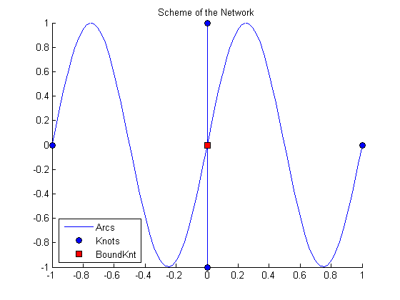
Figure 1: Test 1, structure of the graph.

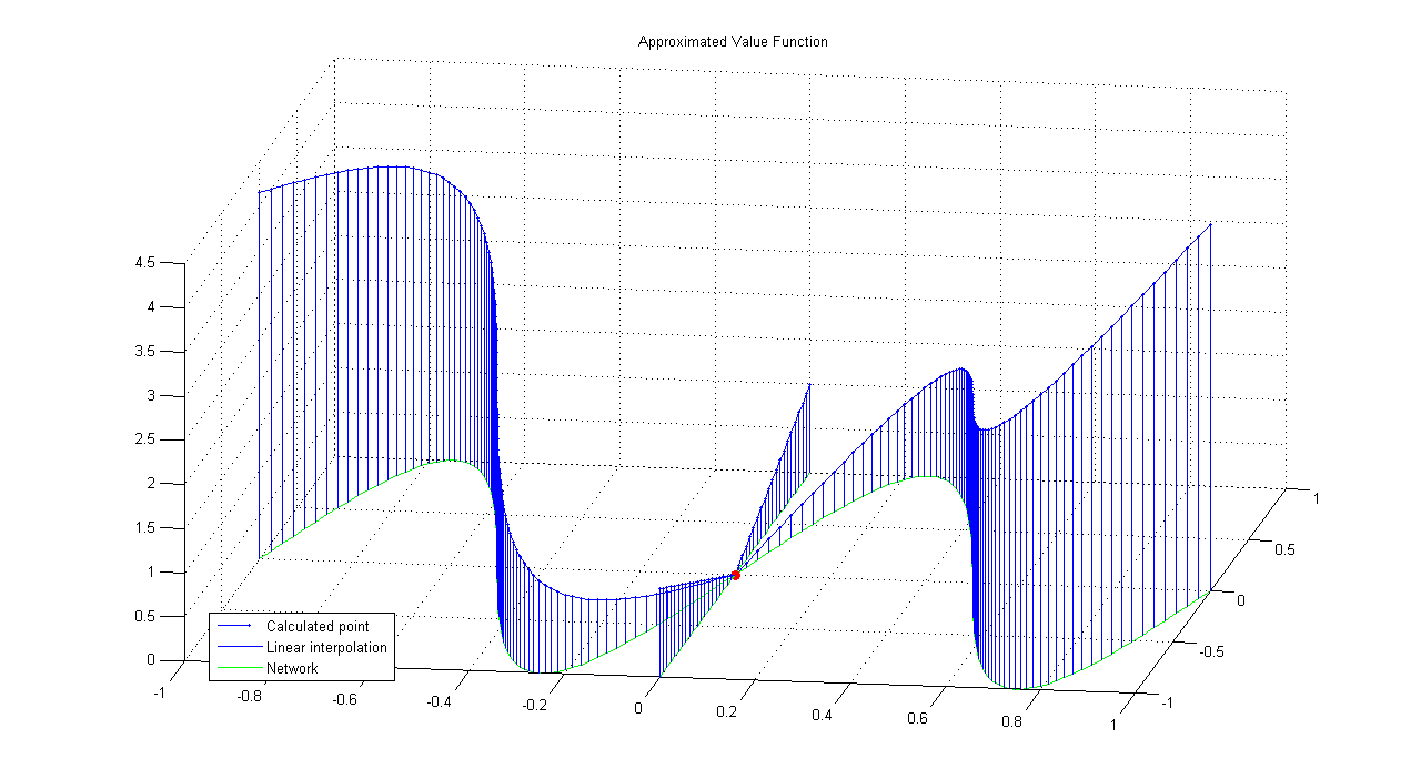
Figure 2: Test 1, $\Delta x=0.025$.

In the first test we consider a five knots graph with two straight arcs and two sinusoidal ones (see figure 1). The only boundary knot is the one placed at the origin and the value of the solution at this knot is fixed to zero. The cost function is constant, i.e. $f(x)\equiv 1$ on $\Gamma$. In this case the correct solution is

$$\begin{split}u(x)=&dist(x,0)=|x_{2}|\quad\hbox{ for the straight arcs}\\ u(x)=&\int^{|x_{1}|}_{0}(\sqrt{1+(2\pi\cos{2\pi t})})dt\quad\hbox{ for sinusoidal arcs}\end{split}$$ (4.4)

An approximated solution is shown in Figure 2. In Table 1, we compare the exact solution with the approximate one, obtained by the scheme. We observe a numerical convergence to the correct solution in $L_{2}$-norm and in the uniform one. As uniform norm we consider the maximum of the uniform norm of the error on every arc and as $L_{2}$-norm the maximum of the $L_{2}$-norm on every arc. We can observe an order of convergence close to $0.5$ that is the typical theoretical order of convergence in the uniform norm of semi-Lagrangian schemes in ${\mathbb{R}}^{n}$, (see for instance [4]).

$\Delta x=h$	$||\cdot||_{\infty}$	$Ord(L_{\infty})$	$||\cdot||_{2}$	$Ord(L_{2})$
0.2	0.1468		0.1007
0.1	0.0901	0.7043	0.0639	0.6562
0.05	0.0630	0.5162	0.0491	0.3801
0.025	0.0450	0.4854	0.0402	0.2885
0.0125	0.0321	0.4874	0.029	0.4711

Table 1: Test 1.

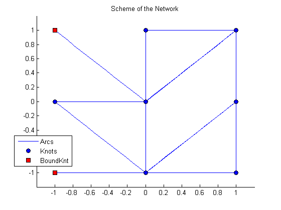
Figure 3: Test 2, structure of the graph.

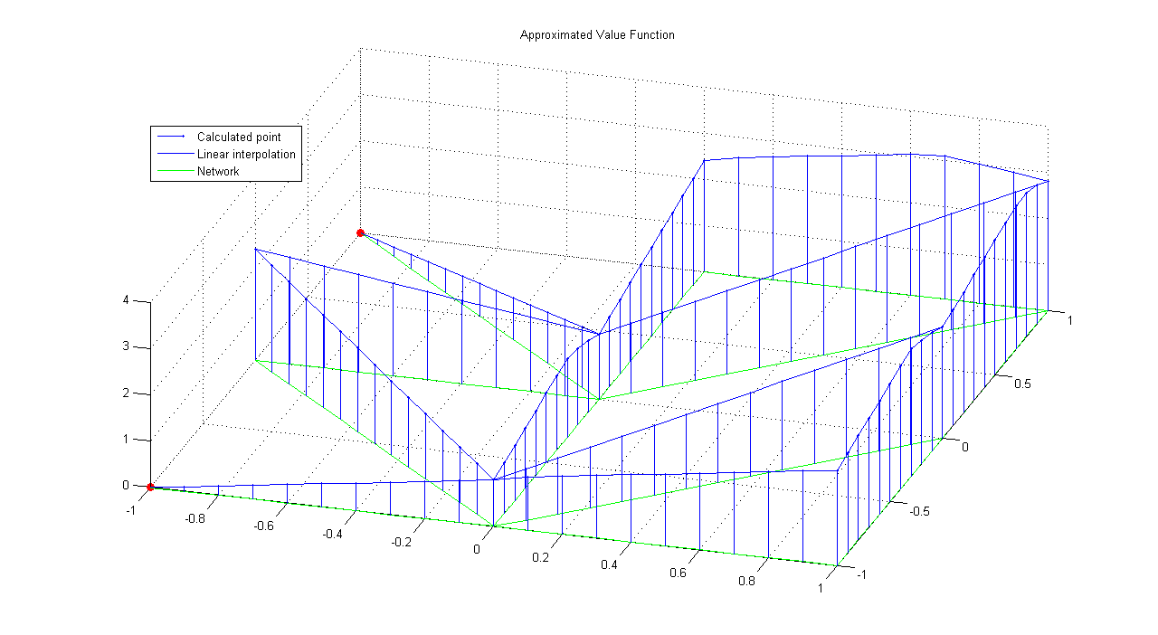
Figure 4: Test 2, $\Delta x=0.1$.

In the second test we present a more complicated graph with two boundary vertices and a several connections among the arcs. Also in this case, we consider a constant cost function $f(x)\equiv 1$ on $\Gamma$. In Table 2 and in Figure 4 we show our results.
In this case we observe an improvement of order of convergence with respect to the previous example. This is due to the fact that the graph is compose of only straight arcs and this reduces the error due to the piecewise linear discretization of the arcs.

$\Delta x=h$	$||\cdot||_{\infty}$	$Ord(L_{\infty})$	$||\cdot||_{2}$	$Ord(L_{2})$
0.2	0.1716		0.0820
0.1	0.0716	1.2610	0.0297	1.4652
0.05	0.0284	1.3341	0.0127	1.2256
0.025	0.0126	1.1611	0.0072	0.8188
0.0125	0.0056	1.1699	0.0037	0.9605

Table 2: Test 2.

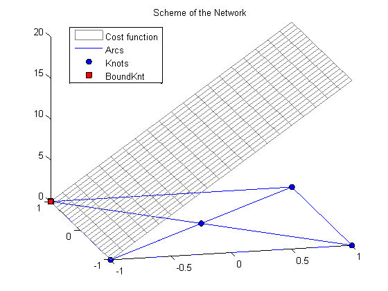
Figure 5: Test 3, structure of the graph.

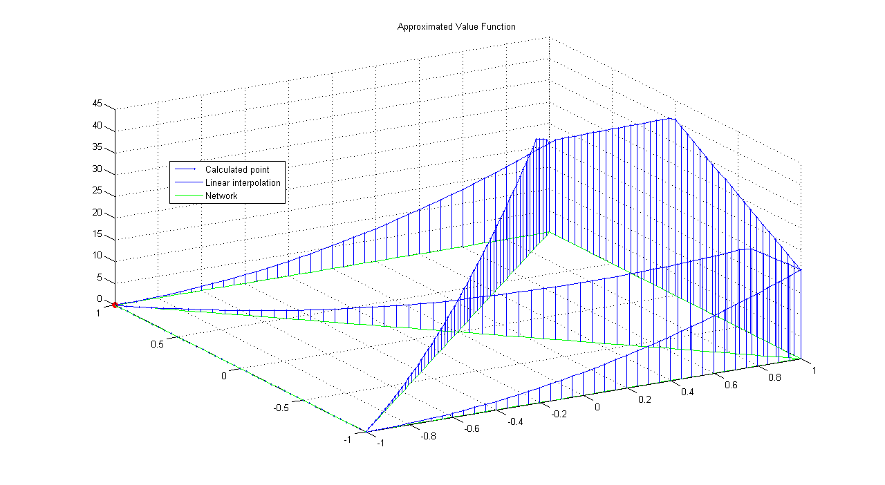
Figure 6: Test 3, $\Delta x=0.05$.

In the third test we consider a five knots graph (figure 5), with a running cost which is not constant. For any point on the graph $x=(x_{1},x_{2})\in\Gamma$, we take $f(x)=10(x_{1}-1)+\eta$, hence $f(x)\geq\eta>0$ for $x\in\Gamma$. In the example, we set $\eta=10^{-10}$. The graph of the approximate solution is shown in Figure 6. Also in this case we provide a experimental table of convergence for the error (Table 3). In absence of an exact solution we compare the approximation for various grid sizes with a discrete solution $U_{ex}$ on a fine grid ($\Delta x=0.005$).

$\Delta x=h$	$||\cdot||_{\infty}$	$Ord(L_{\infty})$	$||\cdot||_{2}$	$Ord(L_{2})$
0.2	0.3800		0.2078
0.1	0.1800	1.078	0.0855	1.2812
0.05	0.08	1.1699	0.0419	1.029
0.025	0.035	1.1926	0.0222	0.9164
0.0125	0.0166	1.0762	0.0103	1.1079

Table 3: Test 3.

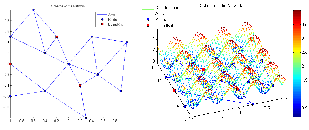
Figure 7: Test 4, structure of the graph.

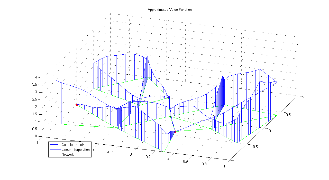
Figure 8: Test 4, $\Delta x=0.05$.

As our last test we consider a graph with several boundary points and a more complicated running cost function $f$. A representation of this graph is shown in Figure 7. We consider the following function $f$

$$f(x_{1},x_{2})=2.1-\sin(4\pi x_{1})+\cos(4\pi x_{2})$$ (4.5)

obviously, because of the regularity of this function, its restriction on the arcs of the graph is continuous.
In Table 4 we show a comparison for the error in various grid steps. Also in this case, in absence of the correct solution, we consider as correct the approximation on a fine grid ($\Delta x=0.005$).

$\Delta x=h$	$||\cdot||_{\infty}$	$Ord(L_{\infty})$	$||\cdot||_{2}$	$Ord(L_{2})$
0.2	0.7049		0.3676
0.1	0.2925	1.2690	0.1557	1.2394
0.05	0.1460	1.0025	0.0777	1.0028
0.025	0.0728	1.0040	0.0320	1.2798
0.0125	0.0375	0.9570	0.0108	1.5670

Table 4: Test 4.

References

- Achdou et al. [2011] Y. Achdou, F. Camilli, A. Cutrì, N. Tchou, Hamilton-jacobi equations constrained on networks, 2011. To appear on NoDEA Nonlinear Differential Equations Appl.
- Bardi and Capuzzo-Dolcetta [1997] M. Bardi, I. Capuzzo-Dolcetta, Optimal Control and Viscosity Solutions of Hamilton-Jacobi-Bellman Equations (Systems & Control: Foundations & Applications), Birkhäuser Boston, 1 edition, 1997.
- Camilli and Siconolfi [1999] F. Camilli, A. Siconolfi, Maximal subsolutions for a class of degenerate hamilton-jacobi problems, Indiana Univ. Math. J. 48 (1999) 1111–31.
- Falcone and Ferretti [2002] M. Falcone, R. Ferretti, Semi-lagrangian schemes for hamilton-jacobi equations, discrete representation formulae and godunov methods, Journal of Computational Physics 175 (2002) 559 –75.
- Fathi and Siconolfi [2005] A. Fathi, A. Siconolfi, Pde aspects of aubry-mather theory for quasiconvex hamiltonians, Calc. Var. Partial Differential Equations 22 (2005) 185–228.
- Garavello and Piccoli [2006] M. Garavello, B. Piccoli, Traffic flow on networks, volume 1 of AIMS Series on Applied Mathematics, American Institute of Mathematical Sciences (AIMS), Springfield, MO, 2006.
- Imbert et al. [2011] C. Imbert, R. Monneau, H. Zidani, A hamilton-jacobi approach to junction problems and application to traffic flows, 2011. To appear on ESAIM Control Optim. Calc. Var.
- Ishii and Mitake [2007] H. Ishii, H. Mitake, Representation formulas for solutions of hamilton-jacobi equations with convex hamiltonians, Indiana Univ. Math. J. 56 (2007) 2159–84.
- Lumer [1980] G. Lumer, Espaces ramifiés, et diffusions sur les réseaux topologiques, C. R. Acad. Sci. Paris Sér. A-B 291 (1980) A627–30.
- Nicaise [1988] S. Nicaise, Elliptic operators on elementary ramified spaces, Integral Equations Operator Theory 11 (1988) 230–57.
- Pokornyi and Borovskikh [2004] Y.V. Pokornyi, A.V. Borovskikh, Differential equations on networks (geometric graphs), J. Math. Sci. (N. Y.) 119 (2004) 691–718.
- Schieborn and Camilli [2011] D. Schieborn, F. Camilli, Viscosity solutions of eikonal equations on topological networks, 2011. To appear on Calc. Var. Partial Differential Equations.