A Comprehensive Study of the ³He-He II Sandwich System Using Monte Carlo Techniques

Abstract

We present a numerical investigation of the thermal and structural properties of the ⁴He-³He sandwich system adsorbed on a graphite substrate using the Worm Algorithm Quantum Monte Carlo (WAQMC) method M. Boninsegni, N. V. Prokof’ev, and B. V. Svistunov (2006a). For this purpose, we modified a previously written WAQMC code originally adapted for ⁴He on graphite, by including the second ³He-component. In order to describe the fermions, a temperature-dependent statistical potential was used which proved very effective. To the best of our knowledge, the statistical potential has not been used before in Quantum Monte Carlo techniques for describing fermions. In an unprecedented task, the WAQMC calculations were conducted in the milli-Kelvin temperature regime. However, because of the heavy computations involved, only 30, 40, and 50 mK were considered for the time being. The pair correlations, Matsubara Green’s function, structure factor, and density profiles were explored at theses temperatures. (Note: this paper is just a preliminary version and will be replaced by an updated version.)

I Introduction

There have been only a few investigations on the ⁴He-³He sandwich system in the last 25 years Humam B. Ghassib and Yahya F. Waqqad (1994); D. McQueeney, G. Agnolet, and J. D. Reppy (1984), most of the studies having concentrated on ⁴He-³He films H. Akimoto and R. B. Hallock (2003); H. Akimoto, J. D. Cummings, and R. B. Hallock (2006); F. Ziouzia, J. Ny$\acute{e}$ki, B. Cowan, and J. Saunders (2003); A. Nash, M. Larson, J. Panek, and N. Mulders (2003); H. B. Ghassib (1984) and superfluid ⁴He films M. Pierce and E. Manousakis (1999); Marlon Pierce and Efstratios Manousakis (2001). These investigations aimed at calculating the Fermi liquid parameters, the speed of third sound in He II, the specific heat capacity, and the Kosterlitz-Thouless (KT) transition. ⁴He-³He mixtures and films E. Krotscheck, J. Paaso, M. Saarela, and K. Schörkhuber (2001); H. B. Ghassib and S. Chatterjee (1984) are considered important physical systems for several reasons: 1) their use in cooling to the milli-Kelvin regime; 2) the central role as theoretical labs for the study of a number of methods in many-body physics; and 3) the importance of the sandwich system specifically in its role where dimensionality effects arise. One can thus see the importance of this study, particularly since it will be conducted using Quantum Monte Carlo techniques. Previous work on ⁴He-³He mixtures and films is abundant. Experimentally, the torsional oscillator was used to study the superfluid ⁴He-³He sandwich system D. McQueeney (1988) and it was found that the critical temperature for the Kosterlitz-Thouless (KT) transition decreases as the number of ³He atoms is increased. Measurements on third sound in ⁴He-³He films have also been conducted. It was found that by increasing the concentration of ³He in ⁴He, the speed of third sound decreases and a complete phase separation occurs at $T\leq 0.5$ K. As a result, this system resembles the ⁴He-³He sandwich system. Ghassib and Waqqad Humam B. Ghassib and Yahya F. Waqqad (1990) reconsidered Bose-Einstein condensation in an ideal, quasi two-dimensional Bose gas and explored crossover effects from two- to three-dimensional systems. Further, Ghassib and Chatterjee H. B. Ghassib and S. Chatterjee (1984) examined the effects of ⁴He impurities on some low-temperature properties of normal liquid ³He. It was argued that no ⁴He-³He mixtures can possibly exist at very low temperature ($T\leq 100$ mK), where a total phase separation occurs.

From another point of view, the possibility for dimer and trimer formation in ⁴He-³He films was explored. Ghassib H. B. Ghassib (1984) predicted that dimers form initially in ³He; afterwards $-$at much lower temperatures$-$ a KT transition could occur for boson composites. ⁴He-³He mixtures in two dimensions have also been considered. For example Krotscheck et al.  E. Krotscheck, J. Paaso, M. Saarela, and K. Schörkhuber (2001) showed than an effective interaction between pairs of ³He atoms inside a host ⁴He liquid was sufficient to cause loosely-bound dimers.

Investigations of ⁴He on a graphite substrate have also been conducted. For example, Corboz et al.  Philppe Corboz, Massimo Boninsegni, Lode Pollet, and Matthias Troyer (2008) investigated the low-temperature phase diagram of the first and second layer of ⁴He adsorbed on graphite, using the worm algorithm. Pierce and Manousakis M. Pierce and E. Manousakis (1999); Marlon Pierce and Efstratios Manousakis (2001) presented a path-integral Monte Carlo (PIMC) method for simulating helium films on the graphite surface, and investigated helium layers adsorbed on the substrate. In addition, diffusion Monte Carlo has also been used to study the first layer of ⁴He adsorbed on graphite M. C. Gordillo and J. Boronat (2009), and the ground-state properties of the homogeneous two-dimensional liquid ⁴He S. Giorgini, J. Boronat, and J. Cassuleras (1996).

It is obvious that these previous investigations are not enough; here here we provide a more comprehensive in depth microscopic study of this system. Our chief goal is to compute some thermal and structural properties of the ⁴He-³He sandwich system in the milli Kelvin temperature regime using the Worm Algorithm Quantum Monte Carlo method M. Boninsegni, N. V. Prokof’ev, and B. V. Svistunov (2006a). To the best of our knowledge, this kind of system has not been simulated before in such a low-temperature regime. Because of the heavy computational aspect of the present simulations, we were only able to obtain results for three temperatures: $T=30$, 40, and 50 mK.

The ⁴He-³He sandwich system proper consists of a ⁴He solid layer of $\sim 3.6\AA$ thickness adsorbed on the walls of a container, above which resides a ⁴He-³He mixture-layer of 7-11 $\AA$ thickness followed by a pure bulk liquid ³He layer. In this paper, we rejuvinate the investigations on this sandwich system which promises richness in physics. We chiefly investigate the thermal properties, such as the pressure, internal energy, entropy, and superfluid density. By using the superfluid density one can detect the role of ³He atoms in the depletion of the superfluid in such a many-body system. In addition, other properties can be obtained such as the solubility of ³He into ⁴He, and the density profiles which show layer promotion upon increasing the number of ³He or ⁴He atoms. Further, the Matsubara Green’s function $G(p,\tau)$ Gerlad D. Mahan (1990) is computed by the numerical implementation of the WAQMC code M. Boninsegni, N. V. Prokof’ev, and B. V. Svistunov (2006a) in order to check for excitations and particle propagation in the sandwich system. Another key point is that we use a statistical potential R. K. Pathria (1996) in order to include real fermionic statistics into the calculations, thereby circumventing the fermion sign problem, which would otherwise arise if we allowed sign-changes corresponding to permutations of the fermions.

We thus consider $N$ ³He and ⁴He atoms with different numeric ratios in a ⁴He-³He sandwich system on graphite. The interactions between the ⁴He atoms and the ⁴He-³He pairs are described by the Aziz potential R. A. Aziz, V. P. S. Nain, J. S. Carley, W. L. Taylor, and G. T. McConville (1979); whereas the ³He atoms interact by the fictitious statistical potential. The Worm-Algorithm Quantum Monte Carlo (WAQMC) method M. Boninsegni, N. V. Prokof’ev, and B. V. Svistunov (2006a) is used to simulate this system. For this purpose, we modified a previously written Worm-Algorithm code Nik specifically designed for ⁴He on graphite, by including a second component (³He) into the code. The use of a statistical potential in the description of fermions in a Monte Carlo simulation is unprecedented, and we hope to be able to convince the reader of its effectiveness.

We found chiefly that the statistical potential is very effective in describing the ³He fermions in a ⁴He environment. The pair correlation function reveals strong correlations between the three pairs of ³He-³He, ⁴He-⁴He, and ⁴He-³He atoms, signalling the presence of different types of clusters. The Matsubara Green’s function demonstrated substantial activity in the system and a condensate fraction as well. The integrated density profiles, taken in a plane perpendicular to the substrate, revealed crystallization of the layers closest to the graphite substrate; whereas disorder is prevalent in the layers father away from the substrate.

The organization of the paper is as follows. In Sec.II we describe the changes we made in the WAQMC code so as to include the ³He component. For this purpose, we needed to recast some of the information in Ref.M. Boninsegni, N. V. Prokof’ev, and B. V. Svistunov (2006a), so that the reader can understand our changes. In Sec.III we present the results of our calculations and discuss them. Finally, in Sec.IV we present our conclusions.

II Method

In this section, we do not explain the WAQMC technique; we only outline our modifications to the code. The WAQMC method has been explained in detail by the inventors of the technique M. Boninsegni, N. V. Prokof’ev, and B. V. Svistunov (2006a). This technique is relatively new and based on conventional path integral Monte Carlo (PIMC) described earlier by the excellent review of David Ceperley D. M. Ceperley (1995). The idea behind the WAQMC method was to make PIMC more efficient by introducing off-diagonal configurations (worms) into the system in addition to the existing diagonal ones. That is, in WAQMC one uses configurations containing both closed (diagonal) world-lines and one open (off-diagonal) world-line (worm). The diagonal configurations contribute to the partition function, hence referred to as the $Z-$sector, whereas the off-diagonal ones to the Matsubara Green’s function, G, hence referred to as the $G-$sector M. Boninsegni, N. V. Prokof’ev, and B. V. Svistunov (2006a). In PIMC as well as WAQMC, each particle is represented by a trajectory in space-time which closes upon itself in space after it has moved for a time $\beta$. Each position in space-time on this trajectory is represented by a bead, and each pair of consecutive beads is separated by a time slice $\tau$. If there are $M$ time slices, then $\beta=M\tau$, where $M$ is the number of time slices along a certain trajectory, the path of the particle in space-time. The particle is thus described by a ring-polymer, an entirely new picture D. M. Ceperley (1995).

II.1 Interactions

For the ⁴He-⁴He and ⁴He-³He interactions, the standard interatomic Aziz potential R. A. Aziz, V. P. S. Nain, J. S. Carley, W. L. Taylor, and G. T. McConville (1979) was used. For the ³He-³He interactions we invoked a fermionic statistical potential R. K. Pathria (1996) given by

$$v_{s}(r)\,=\,-k_{B}T\ln[1-\exp(-2\pi r^{2}/\lambda^{2})],$$ (1)

where $\lambda=\hbar^{2}/(2m)$, $k_{B}$ being Boltzmann’s constant, $r$ the distance between a pair of ³He atoms, and $T$ the temperature. The idea behind the statistical potential is to simulate real fermions; thereby circumventing the sign problem, as mentioned previously.

II.2 Worm updates

In what follows, we describe the changes that we implemented in the WAQMC code in order to include the second ³He component. For this purpose, we recast some of the information in Ref.M. Boninsegni, N. V. Prokof’ev, and B. V. Svistunov (2006a) in order to shed enough light on the changes. All the worm-update equations and concepts used in this paper were given earlier in Ref.M. Boninsegni, N. V. Prokof’ev, and B. V. Svistunov (2006a), except for the indicated changes made to accommodate the ³He component.

The worm updates are accepted or rejected according to certain, carefully defined probabilities. In essence, only one worm is allowed and added to the diagonal configurations. This worm, when inserted, has a starting bead named for historical reasons Masha ($\cal M$), and an ending bead named Ira ($\cal I$). Ira always advances Masha in time. Ira or Masha, that is the end-beads of a worm, can be moved forward or backward in time. They can be reconnected to diagonal trajectories after these trajectories are cut open, and they can also close an off-diagonal trajectory by glueing a worm to the opening. Further, a worm can be erased and then reintroduced. Beads across two different trajectories can be linked together by diagrammatic links, leading to bonds between them.

The WAQMC code was originally written M. Boninsegni, N. V. Prokof’ev, and B. V. Svistunov (2006a) for one component only, namely ⁴He, on graphite. To include the ³He component, a logical array $who_{-}are{}_{-}you(bead)$ was introduced which would return a true value for a chosen bead if it was ⁴He, and false if it was ³He in order to label the particles and to distinguish between them.

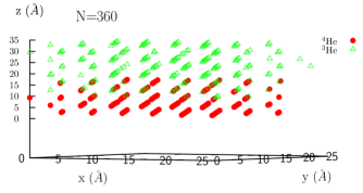
Figure 1: Initialization of a ⁴He-³He sandwich system of $N=360$ atoms on a graphite substrate. The ⁴He atoms (red circles) are adsorbed on a graphite surface constituting a layer of $\sim 3.6\AA$ thickness. The ³He atoms (green triangles) form a bulk layer of about $\sim 7\AA$ thickness. Sandwiched in between these two is a ⁴He-³He mixture-layer of $\sim 15\AA$ thickness. The ratio of ³He and ⁴He atoms in the latter is chosen randomly.

II.2.1 Initialization

The ⁴He-³He sandwich system is initialized using straight world-lines each of length $\beta$ as shown in Fig.1, for a system of, e.g., $N_{3}=222$ ³He atoms and $N_{4}=138$ ⁴He atoms. A logical bead list $who_{-}are{}_{-}you(bead)$ is initialized as the sandwich system is built up into layers on graphite. The first layer adsorbed on the graphite surface consists of ⁴He atoms only constituting about 25$\%$ of the total number of atoms $N$ ($0.25\beta/\epsilon$ beads), the second consists of a ⁴He-³He mixture constituting 25$\%$ of $N$, whereas the third layer consists only of ³He atoms constiuting the rest of $N$. Here, $\epsilon$ is the “time step” in the Worm Algorithm technique. The type of the atoms in the mixture-layer is randomly assigned to simulate a realistically mixed layer.

Figure 2: Worm-Algorithm Insert update representation in space-time coordinates. Ira ($\cal I$) and Masha ($\cal M$) are show as red solid circles.

II.2.2 Insert

A worm, either fermionic or bosonic, is created as shown in Fig.2, where the beginning of the worm is Masha ($\cal M$) and the end Ira ($\cal I$). The figure is a presentation of the open (off-diagonal) trajectory in space-time. The type is assigned randomly using a certain probablity: If a random number, $\xi<0.5$ say, the mass used in the updates will be that of ⁴He; if $\xi\geq 0.5$, the mass is that of ³He. Accordingly, we use in FORTRAN 90

$$\xi=rndm()$$

$$\mathbf{IF}(\xi\,\,\mathbf{.lt.}\,\,0.5)\mathbf{THEN}$$

$$mp\,=\,m4$$

$$\mathbf{ELSEIF}(\xi\,\,\mathbf{.ge.}\,\,0.5)\mathbf{THEN}$$

$$mp\,=\,m3$$

$$\mathbf{ENDIF}$$ (2)

where $mp$ is the mass variable in the program, and $m3$ and $m4$ are the masses of ³He and ⁴He. In the upcoming types of worm updates, the beads, newly created or removed, are assigned the value .TRUE. or .FALSE., respectively, according to the choice of the mass in the INSERT update above. Thus except for the CUT update (see Sec.II.2.9 below), the types of beads and the associated mass used is the same as that chosen initially in the INSERT update.

The acceptance probability for this INSERT update is (as in Ref.M. Boninsegni, N. V. Prokof’ev, and B. V. Svistunov (2006a))

$$P_{in}\,=\,min\left\{1,2CVP\overline{M}\,e^{\Delta U\,+\,\mu M\epsilon}\right\},$$ (3)

where $\Delta U$ is the change in the configurational potential energy of the beads due to the insertion of the worm, $\mu$ the chemical potential, and $\epsilon$ is the time step. Here, $C$ is a constant, $V$ the volume of the system, $M$ the length of the worm proposed which is selected randomly within an interval $[1,\overline{M}]$, and $P=\beta/\epsilon$ is the number of time slices along the path of “length” $\beta$. In the WAQMC code, $P_{in}$ is programmed as follows:

$$P_{in}\,=\,w_{ST}\cdot w_{t}\cdot V\,\frac{\beta}{2}\,\frac{\overline{M}}{2}\,\frac{p_{re}}{p_{in}}\,e^{\mu\epsilon M+\Delta U},$$ (4)

where, $w_{ST}$ controls the worm statistics, $p_{re}$ and $p_{in}$ are fixed attempt probabilities for removing and inserting a worm, respectively, and $w_{t}$ is a weight determined from the total number of beads before and after an update. We multiplied Eqs.(4) and (6) below by $1/p_{f}$ or $1/p_{b}$ for a fermion or boson worm, respectively, where $p_{f}$ is the attempt probability for getting a fermion and $p_{b}=1-p_{f}$ the attempt probability for getting a boson.

II.2.3 Remove

A worm, either fermion or boson, is removed (annihilated) as shown in Fig.3. The type of worm to be removed depends on the mass $mp$ chosen in the INSERT update above. That is, if $mp=m3$, then a fermion worm is removed, otherwise if $mp=m4$ a boson worm. The probability for this update is

$$P_{rm}\,=\,min\left\{1,\frac{e^{\Delta U-\mu\overline{M}\epsilon}}{2CVP\overline{M}}\right\},$$ (5)

and in the WAQMC program it is coded

$$P_{rm}\,=\,\frac{4\,w_{t}\,e^{-\mu\epsilon\overline{M}+\Delta U}\,p_{in}}{w_{ST}\cdot V\cdot\beta\overline{M}p_{re}}.$$ (6)

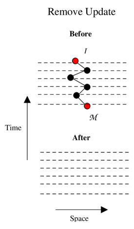
Figure 3: As in Fig.2; but for the removal of a worm.

As a preventive measure during the process of removing the beads, if at any time a bead to be removed has a different type than the worm beads on which the update is performed, the program terminates. But this is just in case and is not supposed to happen.

II.2.4 Move Forward Masha

In this update, the beginning of the worm (timewise speaking slice number 0) is propagated backwards in time as shown in Fig.4. That is to say, a chain of new beads is attached to the old Masha backwards in time ending then with a new Masha. The old Masha is then relabelled as an ordinary bead. In the event that a newly generated bead has a different type than Masha  the program terminates according to the code:

$$\mathbf{IF}(who{}_{-}are{}_{-}you(bead)\mathbf{.ne.}who{}_{-}are{}_{-}you({\cal M}))\mathbf{STOP}$$

(7)

The type of the worm is pre-determined in the INSERT update. The probability for this update advancing Masha forward is

$$P_{ad,\cal M}\,=\,min\left\{1,e^{-\Delta U+\mu M\epsilon}\right\},$$ (8)

and in the program it is coded

$$P_{ad,\,\cal M}\,=\,e^{\mu\epsilon\overline{M}-\Delta U}\cdot w_{t}\cdot w_{lc,\cal M}.$$ (9)

Here $w_{lc,\cal M}$ is the worm-link correction of the links to Masha ($\cal M$):

$$w_{lc_{\cal M}}\,=\,\prod_{i=1}^{N_{\ell}}\,\left(\frac{\displaystyle e^{-\epsilon V(|\mathbf{r}_{\cal M}-\mathbf{r}_{i}|)}-1}{e^{-\epsilon V(|\mathbf{r}_{\cal M}-\mathbf{r}_{i}|)/2}-1}\right),$$ (10)

where $r_{\cal M}$ is the position of Masha, $\mathbf{r}_{i}$ the position of the bead $i$ linked to Masha, $N_{\ell}$ is the number of links to Masha, and $V(r)$ is the pair interaction potential. Here, it doesn’t matter what type of bead one links to since nothing prevents the formation of bonds between fermions and bosons.

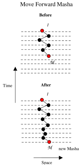
Figure 4: Worm Algorithm update for moving Masha forward

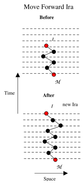
Figure 5: Worm Algorithm update for moving Ira forward.

II.2.5 Move Forward Ira

In this update, the end of the worm (timewise speaking last slice on worm) is propagated forward in time as in Fig.5. Again, the type of worm is pre-determined in the INSERT update, and any newly created beads must have the same type as that of the worm to be updated. If it happens that a bead has a different type than the worm, the program terminates according to

$$\mathbf{IF}(who{}_{-}are{}_{-}you(bead)\mathbf{.ne.}who{}_{-}are{}_{-}you({\cal I}))\mathbf{STOP}.$$

(11)

The probability for this update is

$$P_{ad,\cal I}\,=\,min\left\{1,e^{-\Delta U+\mu M\epsilon}\right\},$$ (12)

and is coded

$$P_{ad,\cal I}\,=\,e^{\mu\epsilon\overline{M}-\Delta U}\cdot w_{t}\cdot w_{lc_{\cal I}}.$$ (13)

Here $w_{lc_{\cal I}}$ is the worm link correction of all the links to Ira

$$w_{lc_{\cal I}}\,=\,\prod_{i=1}^{N_{\ell}}\,\left(\frac{\displaystyle e^{-\epsilon V(|\mathbf{r}_{\cal I}-\mathbf{r}_{i}|)}-1}{e^{-\epsilon V(|\mathbf{r}_{\cal I}-\mathbf{r}_{i}|)/2}-1}\right),$$ (14)

where $\mathbf{r}_{\cal I}$ is the position of $\cal I$ and $N_{\ell}$ is the number of links to $\cal I$.

II.2.6 Move Backward Masha

Here Masha is moved forward in time as in Fig.6. In other words, a chain of new beads is erased forward in time beginning with the old Masha until the erasure stops at a new worm-beginning which becomes then the new Masha. The probability of this update is

$$P_{re,\cal M}\,=\,min\left\{1,e^{\Delta U-\mu M\epsilon}\right\},$$ (15)

and is coded

$$P_{re,\cal M}\,=\,e^{-\mu\epsilon M+\Delta U}w_{lc,{\cal M}}\cdot w_{t}.$$ (16)

As a safety measure, any bead which has a different type than $\cal M$ causes the program to stop, as in (7).

II.2.7 Move Backward Ira

This update moves Ira backward in time as in Fig.7. Correspondingly, a chain of beads is erased backwards in time beginning with the old Ira until the erasure stops at a new Ira. The resulting end of the worm becomes the new Ira. The probability is given by

$$P_{re,\cal I}\,=\,min\left\{1,e^{\Delta U-M\epsilon\mu}\right\},$$ (17)

and is coded:

$$P_{re,\cal I}\,=\,e^{-\mu\epsilon M+\Delta U}\cdot w_{t}\cdot w_{lc,\cal I}.$$ (18)

Again, if a bead happens to have a different type than $\cal I$, the program terminates as in (7) as a safety measure.

II.2.8 Glue

Here, a worm of a type chosen in the INSERT update, is closed to become a ring polymer as shown in Fig.8. Masha and Ira become ordinary beads in this case. The probability for this update is

$$P_{glue}\,=\,min\left\{1,\frac{\rho_{0}(\mathbf{r}_{\cal I},\mathbf{r}_{\cal M},M\epsilon)\,e^{\Delta U+\mu M\epsilon}}{C\overline{M}N_{bd}}\right\},$$ (19)

where $\mathbf{r}_{\cal I}$ and $\mathbf{r}_{\cal M}$ are the positions of $\cal I$ and $\cal M$, respectively, and $N_{bd}$ is the current total number of beads. The free-particle propagator $\rho_{0}$ is given by

$$\rho_{0}(\mathbf{r}_{\cal I},\mathbf{r}_{\cal M},M\epsilon)\,=\,e^{-(\mathbf{r}_{\cal I}-\mathbf{r}_{\cal M})^{2}/(4M\lambda\epsilon)}.$$ (20)

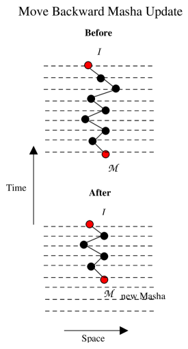
Figure 6: As in Fig.4; but for moving Masha backward

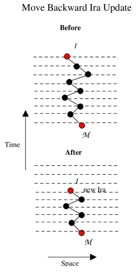
Figure 7: As in Fig.5; but for moving Ira backward.

Eq.(19) is coded

$$P_{glue}\,=\,\left[\frac{1}{4}\,e^{-\mu\epsilon M+\Delta U}e^{-(\mathbf{r}_{\cal I}-\mathbf{r}_{\cal M})^{2}\frac{mp}{2\epsilon M}}(aM)^{3/2}\right.$$

$$\left.(N_{bd}+M-1)w_{ST}\overline{M}\frac{p_{gl}}{p_{cut}}\right.\left.w_{lc,{\cal I}}\cdot w_{lc,{\cal M}}\cdot w_{t})\right]^{-1},$$

where $a\,=\,2\pi\epsilon/mp$, $\mathbf{r}_{\cal I}$ and $\mathbf{r}_{\cal M}$ are the positions of $\cal I$ and $\cal M$, $p_{gl}$ and $p_{cut}$ are the probabilities for attempting a glue or a cut, respectively. The cutting procedure is explained in the next section below. Again, the glue beads must have the same type as the worm beads to be glued, otherwise the program stops using the Fortran statements similar to (7) or (11).

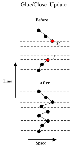
Figure 8: Worm Algorithm update for closing a worm to become a diagonal configuration.

II.2.9 Cut

In this update, a randomly chosen piece of trajectory is removed from a ring polymer in order to create a worm as shown in Fig.9. The beginning of the worm becomes Masha and the end Ira. The mass is assigned according to the type of a randomly chosen bead ($nm$) using the code:

$$\mathbf{IF}(who_{-}are_{-}you(nm)\mathbf{.eq.}\hbox{\bf.TRUE.})\mathbf{THEN}$$

$$mp=m4$$

$$\mathbf{ELSEIF}(who_{-}are_{-}you(nm)\hskip 5.69046pt\mathbf{.eq.}\hbox{\bf.FALSE.})\mathbf{THEN}$$

$$mp=m3$$

$$\mathbf{ENDIF}$$ (21)

The probability for this update is given by

$$P_{cut}\,=\,min\left\{1,\frac{C\overline{M}N_{bd}e^{\Delta U-\mu M\epsilon}}{\rho_{0}(\mathbf{r}_{\cal I},\mathbf{r}_{\cal M},M\epsilon)}\right\},$$ (22)

and is coded

$$P_{cut}\,=\frac{1}{4}\,e^{-\mu\epsilon M+\Delta U}\,e^{(\mathbf{r}_{I}-\mathbf{r}_{M})^{2}\cdot\frac{mp}{2\epsilon M}}(aM)^{3/2}\cdot$$

$$N_{bd}\cdot w_{ST}\overline{M}\cdot\frac{p_{gl}}{p_{cut}}\cdot w_{lc,{\cal I}}\cdot w_{lc,{\cal M}}\cdot w_{t}$$ (23)

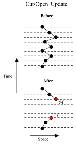
Figure 9: As in Fig.8; but for cutting a ring polymer open, i.e., making a diagonal configuration off-diagonal.

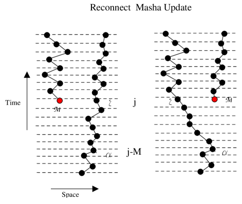
Figure 10: Worm-Algorithm swap updates: After cutting a piece of trajectory between the beads $\alpha$ and $\xi$ from the path to the right of $\cal M$, Masha is reconnected to bead $\alpha$ chosen randomly on the other path, and $\xi$ becomes the new Masha.

II.2.10 Reconnect Masha

In this swap update, Masha of an open world line (worm) and time slice $j$ is connected to a randomly chosen bead $\alpha$ at time $j-M$ on another close world line (ring polymer) as shown in Fig.10, by building a new trajectory between Masha at time $j$ and $\alpha$ at time $j-M$. Prior to this, the trajectory connecting $\alpha$ to a bead $\xi$, where $\xi$ is in the same time slice as Masha, is removed. Again, the mass of each bead is chosen depending on the type of worm inserted in Sec.II.2.2 and to be updated here. We made sure that the swap updates are done between the same type of beads as before:

$$\mathbf{IF}(who_{-}are_{-}you({\cal M})\mathbf{.ne.}who_{-}are_{-}you(\alpha))\mathbf{RETURN}$$

and throughout the removal of the trajectory (i.e., the beads say $\{bead1,\,bead2,\,bead3,\,\cdots,\,beadM\}$ between $\xi$ and $\alpha\equiv bead1$ one checks:

$$\mathbf{IF}(who_{-}are_{-}you(bead1)\mathbf{.ne.}who_{-}are_{-}you(bead2))\mathbf{STOP}$$ (25)

and similarly for the rest of the beads, where $bead2=\mathbf{next}(bead1)$, $bead3=\mathbf{next}(bead2)$ and so on (see M. Boninsegni, N. V. Prokof’ev, and B. V. Svistunov (2006a)). Thus, if a bead does not have the same type as Masha  the update is rejected. If the update is accepted, the previous $\xi$ then becomes the new Masha and the old Masha is connected to $\alpha$. The probability for this update is

$$P_{re,\cal M}\,=\,min\left\{1,e^{-\Delta U}\frac{\Sigma_{\cal M}}{\Sigma_{\xi}}\right\},$$ (26)

where

$$\Sigma_{\cal M}\,=\,\sum_{\sigma\epsilon{\cal L_{M}}}\rho_{0}(\mathbf{r}_{\cal M},\mathbf{r}_{\sigma},\overline{M}\epsilon),$$ (27)

and

$$\Sigma_{\cal\xi}\,=\,\sum_{\sigma\epsilon{\cal L_{M}}}\rho_{0}(\mathbf{r}_{\cal\xi},\mathbf{r}_{\sigma},\overline{M}\epsilon),$$ (28)

with $\cal L_{M}$ the list of particles in the slice $j-M$ in the bins that spatially coincide with the bin of Masha  or one of its nearest neighbors, similarly for $\cal L_{I}$.

The swap probability for Masha is coded

$$P_{re,\cal M}\,=\,\frac{\Sigma_{\cal M}}{\Sigma_{\cal\xi}}\frac{w_{lc,\cal M}}{w_{lc,\cal\xi}}w_{t}e^{-\Delta U}$$ (29)

with

$$\Sigma_{\cal M}\,=\,\left(\frac{1}{\sqrt{aM}}\right)^{3}\,\sum_{i=1}^{h_{m}}e^{-(\mathbf{r}_{\cal M}-\mathbf{r}_{i})^{2}\frac{mp}{2\epsilon M}},$$ (30)

and

$$\Sigma_{\xi}\,=\,\left(\frac{1}{\sqrt{aM}}\right)^{3}\,\sum_{i=1}^{h_{m}}e^{-(\mathbf{r}_{\xi}-\mathbf{r}_{i})^{2}\frac{mp}{2\epsilon M}}.$$ (31)

Here $h_{m}$ is the number of particles in $\cal L_{M}$ and (in the next section) in $\cal L_{I}$.

II.2.11 Reconnect Ira

This is a swap update as in the previous section but for Ira as shown in Fig.11. The probability for this update is given by

$$P_{re,{\cal I}}\,=\,min\left\{1,e^{\Delta U}\,\frac{\Sigma_{\cal I}}{\Sigma_{\xi}}\right\},$$ (32)

where

$$\Sigma_{\cal I}\,=\,\sum_{\sigma\epsilon{L}_{J}}\,\rho_{\sigma}(\mathbf{r}_{I},\mathbf{r}_{\sigma},\overline{M}\epsilon),$$ (33)

and $\Sigma_{\xi}$ was given by Eq.(31) previously. The probability for this update is coded:

$$P_{re,{\cal I}}\,=\,\left(\frac{1}{\sqrt{a\overline{M}}}\right)^{3}\,\frac{\Sigma_{\cal I}}{\Sigma_{\xi}}\frac{w_{lc,\cal I}}{w_{lc,\cal\xi}}\,e^{\Delta U}\,w_{t}\exp(\Delta U).$$ (34)

Again, one makes sure that the swap updates are done on the same type of beads:

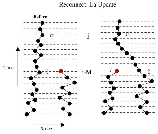
Figure 11: Worm Algorithm swap update: Ira is reconnected to $\alpha$ after removing the trajectory between $\xi$ and $\alpha$. $\xi$ is at the same time as Masha.

$$\mathbf{IF}(who_{-}are_{-}you({\cal I})\mathbf{.ne.}who_{-}are_{-}you(\alpha))\mathbf{STOP},$$ (35)

and during the removal of the path between $\alpha$ and $\xi$

$$\mathbf{IF}(who_{-}are_{-}you(bead1)\mathbf{.ne.}who_{-}are_{-}you(bead2))\mathbf{STOP}.$$ (36)

II.2.12 Insert Link

In addition to the previous updates, this update creates a bond (diagrammatic link) between the beads. In Fig.12, a bond (link) is created between beads $a_{i}$ and $b_{i}$ and the probability for this update is given by:

$$P_{crb}\,=\,\frac{(\overline{M}+1)\,n_{B}}{(\ell_{bnd}+1)\,P_{\cal AB}}\,\left(e^{-fu(\mathbf{r}_{a_{j}}-\mathbf{r}_{b_{j}})}-1\right),$$ (37)

where, $u(\mathbf{r}_{a_{j}}-\mathbf{r}_{b_{j}})$ is the interaction potential between beads $a_{j}$ and $b_{j}$, $n_{B}$ is the number of beads in a spatial bin $\cal B$ within the slice $j$ of the bead $a_{j}$, where the update will be given a try, $\ell_{bnd}$ is the total number of bonds in the initial configuration, and $P_{\cal AB}$ is a probability that depends on the distance between bins $\cal B$ and $\cal A$. The probability is encoded

$$P_{crb}=pat\cdot(e^{-fu(\mathbf{r}_{a_{j}}-\mathbf{r}_{b_{j}})}-1)\frac{\overline{M}+1}{n_{li}\,\cdot\,prob(evk)}$$ (38)

where $n_{li}$ is the total number of links, $pat$ the number of beads $n_{B}$, $prob(evk)$ is $P_{\cal AB}$. Again, the type of bead to which a link is created doesn’t matter. So, we do not check here whether two beads to be linked have the same type or not.

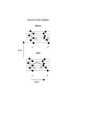
Figure 12: Insert link update: A bead is created between randomly chosen beads $a_{j}$ and $b_{j}$ on different world lines and in the same time slice in their spacial bins $\cal A$ and $\cal B$, respectively.

II.2.13 Remove Link

This update removes a bond between beads $a_{i}$ and $b_{i}$, as shown in Fig.13. The probability for this update is given by

$$P_{rmb}\,=\,\frac{\ell_{bnd}P_{\cal AB}}{(\overline{M}+1)\,n_{B}}\,\left(e^{-fu(\mathbf{r}_{a_{j}}-\mathbf{r}_{b_{j}})}-1\right)^{-1}.$$ (39)

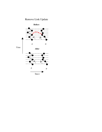
Figure 13: As in Fig.12; but here a bond is removed.

II.2.14 Diagonal

In this update, a randomly chosen piece of trajectory is removed from a closed path and replaced by a newly generated trajectory, as shown in Fig.14. The probability for this update is given by

$$P_{diag}\,=\,e^{-\Delta U}.$$ (40)

The newly generated trajectory must have the same type as the initial diagonal configuration, otherwise the update is rejected.

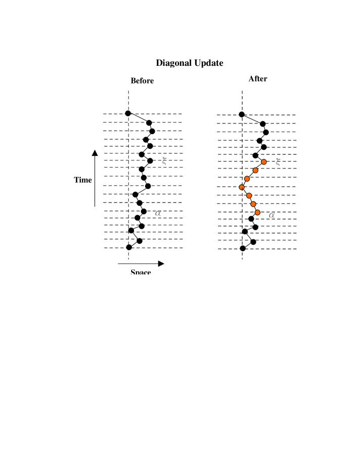
Figure 14: Worm Algorithm Diagonal update where a piece of a trajectory is replace by another one, necessarily of the same type of beads.

II.3 Mobility of ³He in ⁴He

There is an inherent difficulty in the diffusion of ³He atoms in bulk ⁴He. To increase the mobility of ³He inside ⁴He, we applied an approach invented by previous authors Philppe Corboz, Massimo Boninsegni, Lode Pollet, and Matthias Troyer (2008), which makes use of the concept of a fictitous or fake particle. On the other hand, this method also addresses the diffusion of ⁴He atoms in the system. In this technique, one introduces into the system a fake ³He or ⁴He particle whose mass is allowed to vary during the simulation in increments of $\pm dm$. One can then increase the mobility of ³He and ⁴He atoms by reducing their mass or vice versa.

Computationally, an array $markf$ is introduced in order to mark beads as either fake (.FALSE.) or real (.TRUE.). This array is initialized in the beginning to .TRUE.. Next, two mass differences

$$\Delta m_{3}=|m_{fake}-m_{3}|$$

$$\Delta m_{4}=|m_{fake}-m_{4}|$$ (41)

determine whether a fake ³He or ⁴He atom of mass $m_{fake}$ is to be chosen. The mass $m_{fake}$ is initialized to $m_{3}$ and then updated by a subroutine as explained below. If $|\Delta m_{3}|<dm$, where $dm=(m_{4}-m_{3})/10.$, a subroutine choosing a fake ³He particle is called. Otherwise, if $|\Delta m_{4}|<dm$, another subroutine chooses a fake ⁴He particle (see Appendix). When a fake particle is chosen, the beads of its closed trajectory are labelled .FALSE..

II.3.1 Choosing a fake ³He particle

In the subroutine choosing a fake ³He particle, a bead ($bead1$) is selected randomly from a list of beads [$nlist()$]:

$$i=rndm()*nmnm+1;\hskip 14.22636ptip=nlist(i);\hskip 14.22636ptbead1=ip,$$ (42)

where $nmnm$ is the number of beads at some number of Monte Carlo steps. If it happens that ($bead1$) is a ³He atom, a trajectory of length $\beta=Mbeta$ time slices is assigned using a bead-list array $lbfnew()$ starting with $lbfnew(0)=bead1$. Otherwise, if $bead1$ is ⁴He, the routine returns to (42) above and tries again until a ³He $bead1$ is chosen. If the last bead ($ip=lbfnew(Mbeta)$) is not equal to $bead1$, that is the particle is in an exchange cycle, the chosen fake trajectory is rejected, i.e., its beads are not relabelled .FALSE.. The subroutine then returns to Eq.(42) and starts all over again. If all goes well, that is by having a fake and closed pure ³He or ⁴He trajectory, a loop labels the beads of the chosen trajectory by .FALSE. to make it fake:

$$markf=\mathbf{.TRUE.}$$

$$do\hskip 14.22636ptk=0,Mbeta$$

$$lbf(k)=lbfnew(k)$$

$$markf(lbf(k))=\mathbf{.FALSE.}$$

$$enddo$$ (43)

The subroutine choosing a fake ⁴He particle is exactly the same, except for ⁴He. This subroutine is called when $\Delta m_{4}\leq dm$, i.e., when $mfake$ has reached the mass of ⁴He during the mass update described next. Once a fake trajectory is chosen, its mass is updated by a subroutine for changing the mass of the fake particle. Physical properties are then measured when $|\Delta m_{3}|\leq dm$ or $|\Delta m_{4}|\leq dm$. Hence, any trajectory which has $\Delta m_{3}<dm$ or $\Delta m_{4}<dm$ is considered real and can be used to measure physical properties in a given particle number sector. Thus when $\Delta m_{3}<dm$, the routine looks for another ³He atom to put the fake label on, i.e., one looks for the bead which is the same as the current fake, not in exchange cycles and not fake. Once this bead is found, the previous fake labels are dropped and given to the new bead upon which a whole new closed trajectory is labelled fake to which this beads belongs. Similarly, when $\Delta m_{4}<dm$, the same procedure is applied, except that one chooses a fake ⁴He atom. A fake atom is not introduced when a worm is present. That is, one cannot perform these updates on worms, and one cannot have a fake worm. We must nevertheless emphasize that there will always be one fake atom in the configuration, it never disappears. And this fake atom is not part of any exchange cycle.

II.3.2 Mass update

Once a fake trajectory has been selected, its mass is updated using a subroutine (see Appendix) that we wrote for this following Ref.Philppe Corboz, Massimo Boninsegni, Lode Pollet, and Matthias Troyer (2008). In this subroutine, the trajectory mass is incremented or decremented in steps of $dm$, that is,

$$mfake=mold+sgn*dm,$$ (44)

where the sign of the increment, $sgn=\pm 1$, is chosen randomly by the mechanism

$$x=rndm()$$

$$sgn=(-1)**(int(2.*x)),$$

and $mold$ is the fake (old) mass from the previous update. Thus $mfake$ is constantly updated until it becomes either $m_{4}$ or $m_{3}$ within a small margin of error $|\Delta m_{3}|<dm$ or $|\Delta m_{4}|<dm$. In this case, the mass update stops momentarily allowing a measurement of physical properties. Then, a new fake trajectory is selected. We need to emphasize that the previous trajectory is reset to real (.TRUE.) before either one of the subroutines for choosing a fake is called again. That is, no more than one fake trajectory is allowed. Further, inside the subroutine for choosing a fake mass, its mass is not allowed to obtain values less than $m_{3}$ or larger than $m_{4}$. If it reaches one of them, the mass update is rejected and $mfake$ is reset to $mold$. That is $mfake$ must always remain in the interval $[m_{3},m_{4}]$. The mechanism by which the mass update in Eq.(44) is accepted or rejected is according to a certain probability given by

$$P=\exp[\ell_{k}\Delta m/(2\epsilon)]\cdot\exp[\alpha(m\pm\Delta m)]/\exp[\alpha m],$$ (46)

which is actually a modified version of that of Corboz et al.  Philppe Corboz, Massimo Boninsegni, Lode Pollet, and Matthias Troyer (2008) and which proved suitable for our purposes. Here $\ell_{k}$ is defined as

$$\ell_{k}=\sum_{k=1}^{M}\,(\mathbf{r}_{k}-\mathbf{r}_{k-1})^{2},$$ (47)

and $\alpha$ is an adjustable parameter. According to this probability, if $P<1$ and $P>\xi$, where $\xi$ is a random number, the mass update is rejected and the newly proposed fake mass in (44) is set back to the previous one, $m_{fake}=m_{old}$. Otherwise, $m_{fake}$ is assigned the newly proposed value.

II.3.3 Mass histogram

During the above processes, statistics for a mass histogram for the several fake particles are collected in 10 mass bins as was done in Ref.Philppe Corboz, Massimo Boninsegni, Lode Pollet, and Matthias Troyer (2008). This is in order to make sure that the different 10 mass intervals are addressed with almost the same probability. For this purpose, one tunes the $\alpha$ value above such that one gets an almost mass flat histogram.

III Results and Discussion

In this section, we present the results of our simulations. We display the pair correlation function $g(r)$ for the three different temperatures $T=30$, 40, and 50 mK, noting that the correlations weaken as the temperature is reduced to 30 mK. Next, the Matsubara Green’s function Gerlad D. Mahan (1990); M. Boninsegni, N. V. Prokof’ev, and B. V. Svistunov (2006a) reveals the presence of a condensate fraction in the system, whereas the ³He component completely depletes the superfluid. In what follows, we first outline the difficulties which restricted our investigations to only three temperatures.

III.1 Difficulties in the WAQMC Simulations

It was possible to conduct WAQMC simulations on three milli-Kelvin temperatures only. The reasons are as follows. First, in order to reach the milli Kelvin regime $T<100$ mK, one needs to use a large number of “time” slices $\beta$ given by $M\,=\,\beta/\tau$. For our present purposes, we used a time step of $\tau=1/400\,\hbox{K}^{-1}$ and a simulation box of dimensions 19.693 $\AA\times$ 17.054 $\AA\times$ 26.798$\AA$. For example, for $\beta\,=\,(1/0.04)$ K^-1 and $\tau\,=\,(1/400)$ K^-1, one needs $M\,=\,10000$. This is a very large number of time slices for WAQMC, let alone PIMC. Until now, and to the best of our knowledge, no one has ever conducted PIMC calculations below 250 mK because of the considerable computational cost involved. Nevertheless, we decided to take this step to explore the physics of the current system in this difficult regime.

Second, because we used a repulsive statistical potential R. K. Pathria (1996) for the ³He pair interaction, the probabilities for worm updates on the ³He system were lowered substantially (as one can see by inspecting the worm-update probabilities in Sec.II.2, which are governed by the interaction of a worm with the rest of the system). Consider further the substantial large number of ³He atoms present in the current system which provides a large repulsive interaction energy. As a result, the evolution of the current simulated system took a considerable computational time in order to reach thermal equilibrium. The fact that the use of repulsive potentials in the WAQMC method can render the simulation inefficient was already mentioned by Boninsegni et al.  M. Boninsegni, N. V. Prokof’ev, and B. V. Svistunov (2006b). In other words, under these circumstances, the worm updates occur at a significantly lower rate.

Third, the exact adjustment of the chemical potential $\mu$ posed another challenge. The average number of particles $\langle N\rangle$ is allowed to vary by running the WAQMC simulation in the grand canonical ensemble. When the system eventually thermalizes, the number of particles, as determined by $\mu$, stabilizes after a long run or thermal evolution time. It is very difficult to predict the number of particles to which the system would eventually thermalize by guessing $\mu$ from the outset, i.e., the beginning of a simulation. One can only conduct several runs at different $\mu$ and the same $T$ in order to obtain various numbers of particles corresponding to the chemical potentials used. Then, one can construct a “calibration curve” of $\langle N\rangle$ vs. $\mu$ for each $T$ within an acceptable error range of $\langle N\rangle$. That way $\mu$ can be predicted $-$numerically speaking $-$ more reliably for other nearby temperatures. Yet, this procedure is very time-consuming, given that one needs to wait for the system to thermalize for each value of $\mu$ chosen. It could take months to determine the correct $\mu$ with the computational resources that we have currently available. As a result, we chose to conduct a qualitative investigation of this system by running the WAQMC simulations in the canonical ensemble by choosing a reasonable $\mu$. In fact, it was later found that in the milli-Kelvin temperature regime, $N$ turns out to be independent of $\mu$.

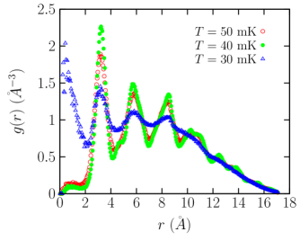
Figure 15: WAQMC pair correlation function $g(r)$ for the ⁴He-³He system at three different temperatures: $T=30$ mK (open circles); 40 mK (solid circles); and 30 mK (open triangles). Distances are in units of $\AA$, and $g(r)$ is in units of $\AA^{-3}$.

III.2 Pair correlations

The correlation function $g(r)$ counts the number of atom pairs with interparticle distance $r$. It provides evidence for the clusterization of particles around certain locations in the system. Fig. 15 displays correlation functions for our system at the indicated temperatures: 50 mK (open circles); 40 mK (solid circles); 30 mK (open triangles). The peaks in this figure strongly indicate the presence of clusters $-$possibly droplets. This explanation is similar to that given by Boninsegni and Szybisz M. Boninsegni and L. Szybisz (2004), who investigated helium films on lithium substrates at $T=0.5$ K. Their $g(r)$ acquires a nonzero value at the origin, indicating that the helium film is forming droplets on the substrate surface. Inspecting Fig. 15, one can see that $g(r=0)=0$ at all $T$. That is, the ⁴He adsorbed on the substrate forms no droplets, as it is almost a solid. The rest of the peaks in $g(r)$ possibly signals the presence of pure ⁴He clusters at $r\sim 3\AA$, ³He-⁴He (pair) clusters at $r\sim 6\AA$, and pure ³He-³He (pair) clusters at $r\sim 8\AA$. This is a reflection of the zero-point motion of ³He and ⁴He, that of ³He being larger, of course. Accordingly, the pure ⁴He cluster would have the lowest interparticle distances around $r\sim 3\AA$. The ³He-⁴He cluster would have larger interparticle distances because of the larger ³He zero-point motion. Finally, the ³He cluster has the largest interparticle distances as it is undergoing only ³He zero-point motion. Yet $g(r)$ in Fig. 15 decays to zero at large $r\geq 16\AA$, the reason being that our system is simulated in a box of finite size and does not extend to infinity. There are some remaining oscillations in $g(r)$ at $r\geq 10\AA$, which could be indicative of other types of structures. However, at $T=30$ mK, $g(r)$ has a peak at $r\sim 0.5\AA$. Some particles may have left the higher layers and approached the graphite surface, most likely ³He. Being attracted by the strong graphite potential, once the ³He atoms reach the surface of the substrate, the strong ³He-graphite interaction ($\sim\,-200$ K) overcomes their zero-point motion ($\sim 7$ K), and they begin to form more ³He or ³He-⁴He clusters close to the surface. Further, the intensity of $g(r)$ at $r\sim 3$, 6, and $8\AA$ indicates clustering closer to the graphite surface, as atoms leave the higher layers and approach the substrate.

A question arises as to the role of temperature reduction on particle promotion and demotion from one layer to another. Are ³He atoms (or ⁴He) being demoted from the highest layer down, closer to the graphite surface? What is the role of the statistical potential in this case? We know that it is temperature-dependent.

III.3 Matsubara Green’s function

In what follows, we explore the possibility for the presence of excitations in the system by measuring the Matsubara Green’s function (MGF) $G(p,\tau)$ Gerlad D. Mahan (1990) at zero momentum using WAQMC. In other words, we check whether our system, as simulated by WAQMC, has really reached its ground state or not. This is a crucial point in the verification of the reliability of the results. Often, in heavy computational techniques like WAQMC, such a step can give the green light for finally stopping the simulation.

Figs. 16, 17, and 18 present the WAQMC $G(p=0,\tau)$ at $T=30$, 40, and 50 mK in the “time” range $-\beta\leq\tau\leq\beta$. The $G(p=0,\tau)$ signal significant activity in the system at the various times $\tau$. The particles seem to propagate at various amplitudes of the MGF in the $p=0$ state at the different values of $\tau$; yet no signals for particle excitations or deexcitations are detected. In fact, the Green function at $\tau=0$ corresponds to the number of particles in the condensate $N_{0}$! That is, according to Mahan Gerlad D. Mahan (1990), $G(p=0,\tau=0)\propto-N_{0}$, where the proportionality sign arises because the Green function obtained in this treatment contains signals from both the fermions and the bosons. Accordingly, one might be tempted to argue that there is a condensate in our system since, at $\tau=0$, the Green function in all three Figs.  16, 17, and 18 displays a nonzero value.

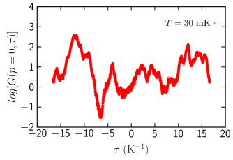
Figure 16: The logarithm of the WAQMC zero-momentum Matsubara Green function $\log[G(p=0,\tau)]$ at $T=30$ mK. The “time” $\tau$ is in units of K^-1.

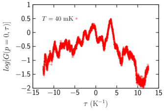
Figure 17: As in Fig. 16; but for $T=40$ mK.

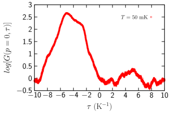
Figure 18: As in Fig. 16; but for $T=50$ mK.

III.4 Structure Factor

Fig. 19 displays the static structure factor $S(k)$ for the sandwich system at $T=30$ mK. Three significant Bragg peaks appear at $k\sim 0.5$, 0.75, and 1.2$\AA^{-1}$, which reveal crystalline order in the system, largely present in the first few ⁴He layers closest to the graphite substrate. The strong attraction of the helium atoms to the graphite forces crystalline order as the ⁴He atoms get adsorbed on the substrate surface. The absence of Bragg peaks in the higher layers is a consequence of the He-graphite potential becoming weaker. As a result, the bulk ³He component is completely disordered.

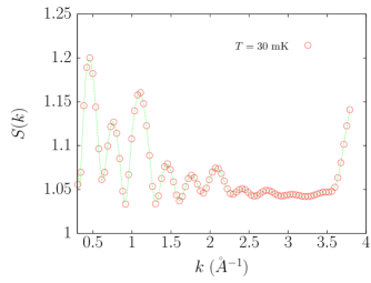
Figure 19: WAQMC static structure factor $S(k)$ at $T=30$ mK. The quasi-momentum wave vector $k$ is in units of $\AA^{-1}$.

III.5 Density Profiles

Figures  20-22 display integrated two-dimensional profiles at $T=30$, 40, and 50 mK, respectively, in the $x-y$ plane perpendicular to the graphite surface $x-z$. The integration is performed along the $z-$axis. A peculiar density distribution is observed at 30 mK, where there is a high peak observed (red cusp), indicating clusterization of the helium atoms. However, it is difficult to tell whether these would be ³He or ⁴He (or both) clusters. Further, there is a smooth, slightly wavy area in the xy plane at $20\leq y\leq 30\AA$ where a crystal structure seems to be absent, and may possibly indicate the presence of a liquid. Figure 21, on the other hand, does not reveal any signals for clusterization at 40 mK. The sharp, periodically ordered peaks are indicative of a largely prevalent crystalline structure. Figure 22 reveals the same absence of crystallization.

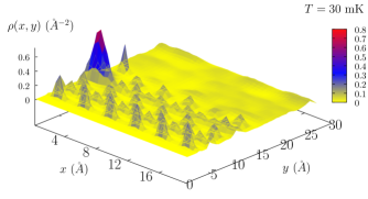
Figure 20: Integrated density $\rho(x,y)$ at $T=$ 30 mK along the $z-$axis in the $xy$ plane perpendicular to the graphite substrate plane

Figure 21: As in Fig. 20; but for 40 mK.

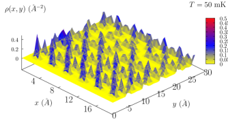
Figure 22: As in Fig. 20; but for 50 mK.

IV Conclusions

In summary, then, the thermal and structural properties of the ³He-⁴He system were investigated at low temperatures in the milli-Kelvin regime. These temperatures lie in an extremely difficult regime in which WAQMC runs must take a long time so as to give good results. The correlations, structure factor, Matsubara Green’s function, and density profiles were explored. A major point in this study is that we used a repulsive statistical potential in order to describe the ³He atoms as real fermions. Although this potential slowed down the evolution of the system during the WAQMC calculation $-$that is, the acceptance probability of worm-updates was reduced and occured less frequently than when using attractive interactions for the ³He atoms $-$ we were still able to evaluate the properties of the system.

It was found that the superfluid fraction of the sandwich has zero value. This is because the large number of ³He atoms depletes the superfluid strongly. The correlation function of the system was evaluated at different temperatures. It was found to display three peaks at $r\sim 3$, 6, and 8$\AA$, signalling ⁴He$-{}^{4}$He, ⁴He$-{}^{3}$He and ³He$-{}^{3}$He clusterizations, respectively. The structure factor was then investigated at $T=30$ mK. It shows a quasicrystalline structure up to $k\sim 2.5\AA^{-1}$; but then disorder sets in. Three significant Bragg peaks appear at $k=0.5$, 0.75, and 1.2$\AA^{-1}$. The density profile of the system was explored at different temperatures. It was shown to depend strongly on temperature. Furthermore, at $T=30$ mK, there is a clustering of the ³He atoms in some region indicated by the highest peak in Fig. 20 In the future, we will explore a few ³He atoms placed on a layer of ⁴He atoms adsorbed on graphite using the same WAQMC code modified here.