Quantized Feedback Control Software Synthesis from System Level Formal Specifications for Buck DC/DC Converters

Abstract

Many Embedded Systems are indeed Software Based Control Systems (SBCSs), that is control systems whose controller consists of control software running on a microcontroller device. This motivates investigation on Formal Model Based Design approaches for automatic synthesis of SBCS control software. In previous works we presented an algorithm, along with a tool QKS implementing it, that from a formal model (as a Discrete Time Linear Hybrid System, DTLHS) of the controlled system (plant), implementation specifications (that is, number of bits in the Analog-to-Digital, AD, conversion) and System Level Formal Specifications (that is, safety and liveness requirements for the closed loop system) returns correct-by-construction control software that has a Worst Case Execution Time (WCET) linear in the number of AD bits and meets the given specifications. In this technical report we present full experimental results on using it to synthesize control software for two versions of buck DC-DC converters (single-input and multi-input), a widely used mixed-mode analog circuit.

1 Introduction

Many Embedded Systems are indeed Software Based Control Systems (SBCSs). An SBCS consists of two main subsystems: the controller and the plant. Typically, the plant is a physical system consisting, for example, of mechanical or electrical devices whereas the controller consists of control software running on a microcontroller. In an endless loop, the controller reads sensor outputs from the plant and sends commands to plant actuators in order to guarantee that the closed loop system (that is, the system consisting of both plant and controller) meets given safety and liveness specifications (System Level Formal Specifications).

Software generation from models and formal specifications forms the core of Model Based Design of embedded software [2]. This approach is particularly interesting for SBCSs since in such a case system level (formal) specifications are much easier to define than the control software behavior itself.

Fig. 1 shows the typical control loop skeleton for an SBCS. Measures from plant sensors go through an AD (analog-to-digital) conversion (quantization) before being processed (line 2) and commands from the control software go through a DA (digital-to-analog) conversion before being sent to plant actuators (line 8). Basically, the control software design problem for SBCSs consists in designing software implementing functions Control_Law and Controllable_Region computing, respectively, the command to be sent to the plant (line 7) and the set of states on which the Control_Law function works correctly (Fault Detection in line 3).

1.  Every $T$ seconds (sampling time) do

2.      Read AD conversion $\hat{x}$ of plant sensor outputs $x$

3.      If ($\hat{x}$ is not in the Controllable_Region)

4.         Then // Exception (Fault Detected):

5.           Start Fault Isolation and Recovery (FDIR)

6.         Else // Nominal case:

7.           Compute (Control_Law) command $\hat{u}$ from $\hat{x}$

8.           Send DA conversion $u$ of $\hat{u}$ to plant actuators

Figure 1: A typical control loop skeleton

In [5] we presented an algorithm and a tool QKS that from the plant model (as a hybrid system), from formal specifications for the closed loop system behaviour (System Level Formal Specifications) and from implementation specifications (that is, number of bits used in the quantization process) can generate correct-by-construction control software satisfying the given specifications.

In this technical report we present full experimental results on using it to synthesize control software for two versions of buck DC-DC converters (single-input and multi-input), a widely used mixed-mode analog circuit.

2 Background

We denote with $[n]$ an initial segment $\{1,\ldots,n\}$ of the natural numbers. We denote with $X$ = $[x_{1},\ldots,x_{n}]$ a finite sequence (list) of variables. By abuse of language we may regard sequences as sets and we use $\cup$ to denote list concatenation. Each variable $x$ ranges on a known (bounded or unbounded) interval ${\cal D}_{x}$ either of the reals or of the integers (discrete variables). We denote with ${\cal D}_{X}$ the set $\prod_{x\in X}{\cal D}_{x}$. To clarify that a variable $x$ is continuous (i.e. real valued) we may write $x^{r}$. Similarly, to clarify that a variable $x$ is discrete (i.e. integer valued) we may write $x^{d}$. Boolean variables are discrete variables ranging on the set $\mathbb{B}$ = {0, 1}. We may write $x^{b}$ to denote a boolean variable. Analogously $X^{r}$ ($X^{d}$, $X^{b}$) denotes the sequence of real (integer, boolean) variables in $X$. Finally, if $x$ is a boolean variable we write $\bar{x}$ for $(1-x)$.

2.1 Predicates

A linear expression over a list of variables $X$ is a linear combination of variables in $X$ with real coefficients. A linear constraint over $X$ (or simply a constraint) is an expression of the form $L(X)\leq b$, where $L(X)$ is a linear expression over $X$ and $b$ is a real constant.

Predicates are inductively defined as follows. A constraint $C(X)$ over a list of variables $X$ is a predicate over $X$. If $A(X)$ and $B(X)$ are predicates over $X$, then $(A(X)\land B(X))$ and $(A(X)\lor B(X))$ are predicates over X. Parentheses may be omitted, assuming usual associativity and precedence rules of logical operators. A conjunctive predicate is a conjunction of constraints. For linear constraints we write: $L(X)\geq b$ for $-L(X)\leq-b$, $L(X)=b$ for (($L(X)\leq b$) $\wedge$ ($-L(X)\leq-b$)) and $a\leq x\leq b$ for $x\geq a\land x\leq b$, being $x\in X$.

A valuation over a list of variables $X$ is a function $v$ that maps each variable $x\in X$ to a value $v(x)$ in ${\cal D}_{x}$. We denote with $X^{\ast}\in{\cal D}_{X}$ the sequence of values $[v(x_{1}),\ldots,v(x_{n})]$. By abuse of language, we call valuation also the sequence of values $X^{\ast}$. A satisfying assignment to a predicate $P$ over $X$ is a valuation $X^{*}$ such that $P(X^{*})$ holds. Abusing notation, we may denote with $P$ the set of satisfying assignments to the predicate $P(X)$. Two predicates $P$ and $Q$ over $X$ are equivalent, notation $P\equiv Q$, if they have the same set of satisfying assignments.

A variable $x\in X$ is said to be bounded in $P$ if there exist $a$, $b\in{\cal D}_{x}$ such that $P(X)$ implies $a\leq x\leq b$. A predicate $P$ is bounded if all its variables are bounded.

Given a constraint $C(X)$ and a fresh boolean variable (guard) $y\not\in X$, the guarded constraint $y\to C(X)$ (if $y$ then $C(X)$) denotes the predicate $((y=0)\lor C(X))$. Similarly, we use $\bar{y}\to C(X)$ (if not $y$ then $C(X)$) to denote the predicate $((y=1)\lor C(X))$. A guarded predicate is a conjunction of either constraints or guarded constraints.

When a guarded predicate is bounded, it can be easily transformed into a conjunctive predicate, as stated by the following proposition.

Proposition 1.

For each bounded guarded predicate $P(X)$, there exists an equivalent bounded conjunctive predicate $Q(X)$.

3 Discrete Time Linear Hybrid Systems

In this section we introduce our class of Discrete Time Linear Hybrid Systems (DTLHS for short).

Definition 1.

A Discrete Time Linear Hybrid System is a tuple ${\cal H}=(X,$ $U,$ $Y,$ $N)$ where:

• $X$ = $X^{r}\cup X^{d}\cup X^{b}$ is a finite sequence of real ($X^{r}$), discrete ($X^{d}$) and boolean ($X^{b}$) present state variables. We denote with $X^{\prime}$ the sequence of next state variables obtained by decorating with ^′ all variables in $X$.

• $U$ = $U^{r}\cup U^{d}\cup U^{b}$ is a finite sequence of input variables.

• $Y$ = $Y^{r}\cup Y^{d}\cup Y^{b}$ is a finite sequence of auxiliary variables. Auxiliary variables are typically used to model modes (e.g., from switching elements such as diodes) or uncontrollable inputs (e.g., disturbances).

• $N(X,U,Y,X^{\prime})$ is a conjunctive predicate over $X\cup U\cup Y\cup X^{\prime}$ defining the transition relation (next state) of the system.

A DTLHS is bounded if predicate $N$ is bounded.

By Prop. 1, any bounded guarded predicate can be transformed into a conjunctive predicate. For the sake of readability, we will use bounded guarded predicates to describe the transition relation of bounded DTLHSs. Note that DTLHSs can effectively model linear algebraic constraints involving both continuous as well as discrete variables. Therefore many embedded control systems may be modeled as DTLHSs.

4 Single-input Buck DC-DC Converter

The buck DC-DC converter (Fig. 2) is a mixed-mode analog circuit converting the DC input voltage ($V_{in}$ in Fig. 2) to a desired DC output voltage ($v_{O}$ in Fig. 2). As an example, buck DC-DC converters are used off-chip to scale down the typical laptop battery voltage (12-24) to the just few volts needed by the laptop processor (e.g. [8]) as well as on-chip to support Dynamic Voltage and Frequency Scaling (DVFS) in multicore processors (e.g. [3, 7]). Because of its widespread use, control schemas for buck DC-DC converters have been widely studied (e.g. see [3, 7, 8, 9]). The typical software based approach (e.g. see [8]) is to control the switch $u$ in Fig. 2 (typically implemented with a MOSFET) with a microcontroller.

\begin{picture}(7611.0,3278.0)(1336.0,-3759.0)\end{picture}

Figure 2: Single-input buck DC-DC converter

Designing the software to run on the microcontroller to properly actuate the switch is the control software design problem for the buck DC-DC converter in our context.

The circuit in Fig. 2 can be modeled as a DTLHS ${\cal H}$ = ($X$, $U$, $Y$, $N$). The circuit state variables are $i_{L}$ and $v_{C}$. However we can also use the pair $i_{L}$, $v_{O}$ as state variables in ${\cal H}$ model since there is a linear relationship between $i_{L}$, $v_{C}$ and $v_{O}$, namely: $v_{O}\;=\;\frac{r_{C}R}{r_{C}+R}i_{L}+\frac{R}{r_{C}+R}v_{C}$. Such considerations lead to use the following sets of variables to model ${\cal H}$: $X$ $=$ $X^{r}$ $=$ $[i_{L}$, $v_{O}]$, $U$ $=$ $U^{b}$ $=$ $[u]$, $Y$ $=$ $Y^{r}\cup Y^{b}$ with $Y^{r}$ $=$ $[i_{u}$, $v_{u}$, $i_{D}$, $v_{D}]$ and $Y^{b}$ $=$ $[q]$. Note how ${\cal H}$ auxiliary variables $Y$ stem from the constitutive equations of the switching elements (i.e. the switch $u$ and the diode D in Fig. 2). From a simple circuit analysis (e.g. see [4]) we have the following equations:

$$\dot{i_{L}} = a_{1,1}i_{L}+a_{1,2}v_{O}+a_{1,3}v_{D}$$ (1)

$$\dot{v_{O}} = a_{2,1}i_{L}+a_{2,2}v_{O}+a_{2,3}v_{D}$$ (2)

where the coefficients $a_{i,j}$ depend on the circuit parameters $R$, $r_{L}$, $r_{C}$, $L$ and $C$ in the following way: $a_{1,1}=-\frac{r_{L}}{L}$, $a_{1,2}=-\frac{1}{L}$, $a_{1,3}=-\frac{1}{L}$, $a_{2,1}=\frac{R}{r_{c}+R}[-\frac{r_{c}r_{L}}{L}+\frac{1}{C}]$, $a_{2,2}=\frac{-1}{r_{c}+R}[\frac{r_{c}R}{L}+\frac{1}{C}]$, $a_{2,3}=-\frac{1}{L}\frac{r_{c}R}{r_{c}+R}$. Using a discrete time model with sampling time $T$ (writing $x^{\prime}$ for $x(t+1)$) we have:

$${i_{L}}^{\prime} = (1+Ta_{1,1})i_{L}+Ta_{1,2}v_{O}+Ta_{1,3}v_{D}$$ (3)

$${v_{O}}^{\prime} = Ta_{2,1}i_{L}+(1+Ta_{2,2})v_{O}+Ta_{2,3}v_{D}.$$ (4)

The algebraic constraints stemming from the constitutive equations of the switching elements are the following:

$\displaystyle q$ $\displaystyle\rightarrow$ $\displaystyle v_{D}=R_{\rm on}i_{D}$ (5) $\displaystyle q$ $\displaystyle\rightarrow$ $\displaystyle i_{D}\geq 0$ (6) $\displaystyle u$ $\displaystyle\rightarrow$ $\displaystyle v_{u}=R_{\rm on}i_{u}$ (7) $\displaystyle v_{D}$ $\displaystyle=$ $\displaystyle v_{u}-V_{in}$ (8)

$\displaystyle\bar{q}$ $\displaystyle\rightarrow$ $\displaystyle v_{D}=R_{\rm off}i_{D}$ (9) $\displaystyle\bar{q}$ $\displaystyle\rightarrow$ $\displaystyle v_{D}\leq 0$ (10) $\displaystyle\bar{u}$ $\displaystyle\rightarrow$ $\displaystyle v_{u}=R_{\rm off}i_{u}$ (11) $\displaystyle i_{D}$ $\displaystyle=$ $\displaystyle i_{L}-i_{u}$ (12)

The transition relation $N$ of ${\cal H}$ is given by the conjunction of the constraints in Eqs. (3)–(12) and the following explicit (safety) bounds: $-4\leq i_{L}\leq 4\land-1\leq v_{O}\leq 7\land-10^{3}\leq i_{D}\leq 10^{3}\land-10^{3}\leq i_{u}\leq 10^{3}\land-10^{7}\leq v_{u}\leq 10^{7}\land-10^{7}\leq v_{D}\leq 10^{7}$.

4.1 Modelling Robustness on Input $V_{in}$ and Load $R$

In this section we address the problem of refining the model given in Sect. 4 so as to require a controller for our single-input buck to be robust to foreseen variations in the load $R$ and in the power supply $V_{in}$. That is, given tolerances $\rho_{R}$ and $\rho_{V_{in}}$, we want the controller output by QKS for our single-input buck to work for any $R\in[\max\{0,R(1-\rho_{R})\},R(1+\rho_{R})]$ and any ${V_{in}}\in[\max\{0,{V_{in}}(1-\rho_{V_{in}})\},{V_{in}}(1+\rho_{V_{in}})]$.

Variations in the power supply are modeled by replacing Eq. (8) in Sect. 4 with the following:

$\displaystyle v_{D}\leq v_{u}-V_{in}(1-\rho_{V_{in}})$ (13)

$\displaystyle v_{D}\geq v_{u}-V_{in}(1+\rho_{V_{in}})$ (14)

Along the same lines, we may model also variations in the load $R$. However, since $N$ dynamics is not linear in $R$, much more work is needed (along the lines of [1]). To this aim, we proceed as follows.

The only equation depending on $R$ is Eq. (4) of Sect. 4. Consider constants $a_{2,1}(R)=\frac{R}{r_{c}+R}[-\frac{r_{c}r_{L}}{L}+\frac{1}{C}]$, $a_{2,2}(R)=\frac{-1}{r_{c}+R}[\frac{r_{c}R}{L}+\frac{1}{C}]$, $a_{2,3}(R)=-\frac{1}{L}\frac{r_{c}R}{r_{c}+R}$ as (nonlinear) functions of $R$. It is easy to see that $a_{2,1}(R)$, $a_{2,2}(R)$ are monotonically increasing functions for $R\in\mathbb{R}^{+}$, while $a_{2,3}(R)$ is monotonically decreasing for $R\in\mathbb{R}^{+}$. Thus, if signs of $i_{L},v_{O},v_{D}$ are known, it is possible to replace Eq. (4) with two inequalities $v_{O}\geq Ta_{2,1}(R_{i_{L}}^{-})i_{L}+(1+Ta_{2,2}(R_{v_{O}}^{-}))v_{O}+Ta_{2,3}(R_{v_{D}}^{-})v_{D}$ and $v_{O}\leq Ta_{2,1}(R_{i_{L}}^{+})i_{L}+(1+Ta_{2,2}(R_{v_{O}}^{+}))v_{O}+Ta_{2,3}(R_{v_{D}}^{+})v_{D}$, being

• $R_{w}^{-}=$ if $w\geq 0$ then $R(1-\rho_{R})$ else $R(1+\rho_{R})$ and $R_{w}^{+}=$ if $w\geq 0$ then $R(1+\rho_{R})$ else $R(1-\rho_{R})$ for $w\in\{i_{L},v_{O}\}$;

• $R_{v_{D}}^{-}=$ if $v_{D}\geq 0$ then $R(1+\rho_{R})$ else $R(1-\rho_{R})$ and $R_{v_{D}}^{+}=$ if $v_{D}\geq 0$ then $R(1-\rho_{R})$ else $R(1+\rho_{R})$.

This leads us to replace Eq. (4) of Sect. 4 with the equations in Fig. 3.

$\displaystyle z_{i_{L}}$ $\displaystyle\to$ $\displaystyle i_{L}\geq 0$ (15) $\displaystyle z_{v_{O}}$ $\displaystyle\to$ $\displaystyle v_{O}\geq 0$ (16) $\displaystyle z_{v_{D}}$ $\displaystyle\to$ $\displaystyle v_{D}\geq 0$ (17) $\displaystyle\overline{z_{i_{L}}}$ $\displaystyle\to$ $\displaystyle i_{L}\leq 0$ (18) $\displaystyle\overline{z_{v_{O}}}$ $\displaystyle\to$ $\displaystyle v_{O}\leq 0$ (19) $\displaystyle\overline{z_{v_{D}}}$ $\displaystyle\to$ $\displaystyle v_{D}\leq 0$ (20) $\displaystyle\overline{z_{ppp}}$ $\displaystyle\to$ $\displaystyle 1-z_{i_{L}}+1-z_{v_{O}}+1-z_{v_{D}}\geq 1$ (21) $\displaystyle\overline{z_{pnp}}$ $\displaystyle\to$ $\displaystyle 1-z_{i_{L}}+z_{v_{O}}+1-z_{v_{D}}\geq 1$ (22) $\displaystyle\overline{z_{ppn}}$ $\displaystyle\to$ $\displaystyle 1-z_{i_{L}}+1-z_{v_{O}}+z_{v_{D}}\geq 1$ (23) $\displaystyle\overline{z_{pnn}}$ $\displaystyle\to$ $\displaystyle 1-z_{i_{L}}+z_{v_{O}}+z_{v_{D}}\geq 1$ (24) $\displaystyle\overline{z_{npp}}$ $\displaystyle\to$ $\displaystyle z_{i_{L}}+1-z_{v_{O}}+1-z_{v_{D}}\geq 1$ (25) $\displaystyle\overline{z_{nnp}}$ $\displaystyle\to$ $\displaystyle z_{i_{L}}+z_{v_{O}}+1-z_{v_{D}}\geq 1$ (26) $\displaystyle\overline{z_{npn}}$ $\displaystyle\to$ $\displaystyle z_{i_{L}}+1-z_{v_{O}}+z_{v_{D}}\geq 1$ (27) $\displaystyle\overline{z_{nnn}}$ $\displaystyle\to$ $\displaystyle z_{i_{L}}+z_{v_{O}}+z_{v_{D}}\geq 1$ (28) $\displaystyle z_{ppp}$ $\displaystyle\to$ $\displaystyle v_{O}^{\prime}\leq Ta_{2,1}^{(M)}i_{L}+(Ta_{2,2}^{(M)}+1)v_{O}+Ta_{2,3}^{(m)}v_{D}$ (29) $\displaystyle z_{ppp}$ $\displaystyle\to$ $\displaystyle v_{O}^{\prime}\geq Ta_{2,1}^{(m)}i_{L}+(Ta_{2,2}^{(m)}+1)v_{O}+Ta_{2,3}^{(M)}v_{D}$ (30) $\displaystyle z_{ppn}$ $\displaystyle\to$ $\displaystyle v_{O}^{\prime}\leq Ta_{2,1}^{(M)}i_{L}+(Ta_{2,2}^{(M)}+1)v_{O}+Ta_{2,3}^{(M)}v_{D}$ (31) $\displaystyle z_{ppn}$ $\displaystyle\to$ $\displaystyle v_{O}^{\prime}\geq Ta_{2,1}^{(m)}i_{L}+(Ta_{2,2}^{(m)}+1)v_{O}+Ta_{2,3}^{(m)}v_{D}$ (32) $\displaystyle z_{pnp}$ $\displaystyle\to$ $\displaystyle v_{O}^{\prime}\leq Ta_{2,1}^{(M)}i_{L}+(Ta_{2,2}^{(m)}+1)v_{O}+Ta_{2,3}^{(m)}v_{D}$ (33) $\displaystyle z_{pnp}$ $\displaystyle\to$ $\displaystyle v_{O}^{\prime}\geq Ta_{2,1}^{(m)}i_{L}+(Ta_{2,2}^{(M)}+1)v_{O}+Ta_{2,3}^{(M)}v_{D}$ (34) $\displaystyle z_{pnn}$ $\displaystyle\to$ $\displaystyle v_{O}^{\prime}\leq Ta_{2,1}^{(M)}i_{L}+(Ta_{2,2}^{(m)}+1)v_{O}+Ta_{2,3}^{(M)}v_{D}$ (35) $\displaystyle z_{pnn}$ $\displaystyle\to$ $\displaystyle v_{O}^{\prime}\geq Ta_{2,1}^{(m)}i_{L}+(Ta_{2,2}^{(M)}+1)v_{O}+Ta_{2,3}^{(m)}v_{D}$ (36) $\displaystyle z_{npp}$ $\displaystyle\to$ $\displaystyle v_{O}^{\prime}\leq Ta_{2,1}^{(m)}i_{L}+(Ta_{2,2}^{(M)}+1)v_{O}+Ta_{2,3}^{(m)}v_{D}$ (37) $\displaystyle z_{npp}$ $\displaystyle\to$ $\displaystyle v_{O}^{\prime}\geq Ta_{2,1}^{(M)}i_{L}+(Ta_{2,2}^{(m)}+1)v_{O}+Ta_{2,3}^{(M)}v_{D}$ (38) $\displaystyle z_{npn}$ $\displaystyle\to$ $\displaystyle v_{O}^{\prime}\leq Ta_{2,1}^{(m)}i_{L}+(Ta_{2,2}^{(M)}+1)v_{O}+Ta_{2,3}^{(M)}v_{D}$ (39) $\displaystyle z_{npn}$ $\displaystyle\to$ $\displaystyle v_{O}^{\prime}\geq Ta_{2,1}^{(M)}i_{L}+(Ta_{2,2}^{(m)}+1)v_{O}+Ta_{2,3}^{(m)}v_{D}$ (40) $\displaystyle z_{nnp}$ $\displaystyle\to$ $\displaystyle v_{O}^{\prime}\leq Ta_{2,1}^{(m)}i_{L}+(Ta_{2,2}^{(m)}+1)v_{O}+Ta_{2,3}^{(m)}v_{D}$ (41) $\displaystyle z_{nnp}$ $\displaystyle\to$ $\displaystyle v_{O}^{\prime}\geq Ta_{2,1}^{(M)}i_{L}+(Ta_{2,2}^{(M)}+1)v_{O}+Ta_{2,3}^{(M)}v_{D}$ (42) $\displaystyle z_{nnn}$ $\displaystyle\to$ $\displaystyle v_{O}^{\prime}\leq Ta_{2,1}^{(m)}i_{L}+(Ta_{2,2}^{(m)}+1)v_{O}+Ta_{2,3}^{(M)}v_{D}$ (43) $\displaystyle z_{nnn}$ $\displaystyle\to$ $\displaystyle v_{O}^{\prime}\geq Ta_{2,1}^{(M)}i_{L}+(Ta_{2,2}^{(M)}+1)v_{O}+Ta_{2,3}^{(m)}v_{D}$ (44)

Figure 3: DTLHS Buck Model Robust on $R$

Note that, w.r.t. the model in Sect. 4, in Fig. 3 we add to $Y^{b}$ 11 auxiliary boolean variables $z_{i_{L}}$, $z_{v_{O}}$, $z_{v_{D}}$, $z_{ppp}$, $z_{ppp}$, $z_{ppn}$, $z_{ppn}$, $z_{pnp}$, $z_{pnp}$, $z_{pnn}$, $z_{pnn}$, $z_{npp}$, $z_{npp}$, $z_{npn}$, $z_{npn}$, $z_{nnp}$, $z_{nnp}$, $z_{nnn}$, $z_{nnn}$ with the following meaning. The boolean variable $z_{i_{L}}$ [$z_{v_{O}}$, $z_{v_{D}}$] is true iff $i_{L}$ [${v_{O}}$, ${v_{D}}$] is positive (see Eqs. (15) and (18) [Eqs. (16) and (19), Eqs. (17) and (20)]). The boolean variable $z_{abc}$, with $a,b,c\in\{p,n\}$, is true iff $($if $a=p$ then $i_{L}\geq 0$ else $i_{L}\leq 0)\land($if $b=p$ then $v_{O}\geq 0$ else $v_{O}\leq 0)\land($if $c=p$ then $v_{D}\geq 0$ else $v_{D}\leq 0)$. This is stated by Eqs. (21)–(28). Finally, we use boolean variables $z_{abc}$ as guards for the inequalities replacing Eq. (4) as stated before. This is done in Eqs. (29)–(44).

5 Multi-input Buck DC-DC Converter

A multi-input buck DC-DC converter [6] (Fig. 4), consists of $n$ power supplies with voltage values $V_{1}<\ldots<V_{n}$, $n$ switches with voltage values $v_{1}^{u},\ldots,v_{n}^{u}$ and current values $I_{1}^{u},\ldots,I_{n}^{u}$, and $n$ input diodes $D_{0},\ldots,D_{n-1}$ with voltage values $v_{0}^{D},\ldots,v_{n-1}^{D}$ and current values $i_{0}^{D},\ldots,i_{n-1}^{D}$ (in the following, we will also write $v_{D}$ for $v_{0}^{D}$ and $i_{D}$ for $i_{0}^{D}$). As for the converter in Sect. 4, the state variables are $i_{L}$ and $v_{O}$. Differently from the converter in Sect. 4, the action variables are $u_{1},\ldots,u_{n}$, thus a control software for the $n$-input buck dc-dc converter has to properly actuate the switches $u_{1},\ldots,u_{n}$.

Figure 4: Multi-input Buck DC-DC converter

We model our $n$-input buck DC-DC converter with DTLHS ${\cal H}$ = ($X,$ $U,$ $Y,$ $N$), where $X=X^{r}=[i_{L},$ $v_{O}],$ $U=U^{b}=[u_{1},$ $\ldots,$ $u_{n}],$ and $Y=Y^{r}\cup Y^{b}$ with $Y^{r}=[v_{D},$ $v_{1}^{D},$ $\ldots,v_{n-1}^{D},$ $i_{D},$ $I_{1}^{u},$ $\ldots,$ $I_{n}^{u},$ $v_{1}^{u},$ $\ldots,$ $v_{n}^{u}]$ and $Y^{b}=[q_{0},$ $\ldots,$ $q_{n-1}]$. As for the predicate $N$, from a simple circuit analysis (e.g. see [4]) we have that state variables constraints are the same as Eqs. (3) and (4) of the converter in Sect. 4.

The algebraic constraints stemming from the constitutive equations of the switching elements are the following (where $i$ and $j$ range in $[n-1]$ and $[n]$ respectively):

$\displaystyle q_{0}$ $\displaystyle\rightarrow$ $\displaystyle v_{D}=R_{\rm on}i_{D}$ (45) $\displaystyle q_{0}$ $\displaystyle\rightarrow$ $\displaystyle i_{D}\geq 0$ (46) $\displaystyle q_{i}$ $\displaystyle\rightarrow$ $\displaystyle v_{i}^{D}=R_{\rm on}I_{i}^{u}$ (47) $\displaystyle q_{i}$ $\displaystyle\rightarrow$ $\displaystyle I_{i}^{u}\geq 0$ (48) $\displaystyle u_{j}$ $\displaystyle\rightarrow$ $\displaystyle v_{j}^{u}=R_{\rm on}I_{j}^{u}$ (49) $\displaystyle i_{L}$ $\displaystyle=$ $\displaystyle i_{D}+\sum_{i=1}^{n}I_{i}^{u}$ (50)

$\displaystyle\bar{q}_{0}$ $\displaystyle\rightarrow$ $\displaystyle v_{D}=R_{\rm off}i_{D}$ (51) $\displaystyle\bar{q}_{0}$ $\displaystyle\rightarrow$ $\displaystyle v_{D}\leq 0$ (52) $\displaystyle\bar{q}_{i}$ $\displaystyle\rightarrow$ $\displaystyle v_{i}^{D}=R_{\rm off}I_{i}^{u}$ (53) $\displaystyle\bar{q}_{i}$ $\displaystyle\rightarrow$ $\displaystyle v_{i}^{D}\leq 0$ (54) $\displaystyle\bar{u}_{j}$ $\displaystyle\rightarrow$ $\displaystyle v_{j}^{u}=R_{\rm off}I_{j}^{u}$ (55) $\displaystyle v_{D}$ $\displaystyle=$ $\displaystyle v_{i}^{u}+v_{i}^{D}-V_{i}$ (56) $\displaystyle v_{D}$ $\displaystyle=$ $\displaystyle v_{n}^{u}-V_{n}$ (57)

Finally, $N$ is given by the conjunction of Eqs. (3) and (4) of Sect. 4, Eqs. (45)–(57) and the following explicit (safety) bounds: $-4\leq i_{L}\leq 4\land-1\leq v_{O}\leq 7\land-10^{3}\leq i_{D}\leq 10^{3}\land\;\bigwedge_{i=1}^{n}-10^{3}\leq I_{i}^{u}\leq 10^{3}\land\;\bigwedge_{i=1}^{n}-10^{7}\leq v_{i}^{u}\leq 10^{7}\land\;\bigwedge_{i=0}^{n-1}-10^{7}$ $\leq v_{i}^{D}\leq 10^{7}$.

5.1 Modelling Robustness on Inputs $V_{i}$ and Load $R$

In this section we address the problem of refining the model given in Sect. 5 so as to require a controller for our multi-input buck to be robust to foreseen variations in the load $R$ and in the power supplies $V_{i}$ (for $i\in[n]$). As it is explained in Sect. 4.1, given tolerances $\rho_{R}$ and $\rho_{V_{i}}$ (for $i\in[n]$), we want the controller output by QKS for our multi-input buck to work for any $R\in[\max\{0,R(1-\rho_{R})\},R(1+\rho_{R})]$ and any ${V_{i}}\in[\max\{0,{V_{i}}(1-\rho_{V_{i}})\},{V_{i}}(1+\rho_{V_{i}})]$ (for $i\in[n]$).

Variations in the power supplies are modeled by replacing Eqs. (56) and (57) in Sect. 5 with the following (where $i$ ranges in $[n-1]$):

$\displaystyle v_{D}\leq v_{i}^{u}+v_{i}^{D}-V_{i}(1-\rho_{V_{i}})$ (58) $\displaystyle v_{D}\geq v_{i}^{u}+v_{i}^{D}-V_{i}(1+\rho_{V_{i}})$ (59)

$\displaystyle v_{D}\leq v_{n}^{u}-V_{n}(1-\rho_{V_{n}})$ (60) $\displaystyle v_{D}\geq v_{n}^{u}-V_{n}(1+\rho_{V_{n}})$ (61)

As for the robustness w.r.t. the load $R$, since the only equation depending on $R$ is Eq. (4) of Sect. 4, which also holds for the multi-input buck, the same reasoning of Sect. 4.1 may be applied. Thus, we have to replace Eq. (4) of Sect. 4 with the equations in Fig. 3.

6 Experimental Results

In this section we present our experimental results about running QKS [5] on the buck models described in Sects. 4 and 5. Namely, we will present experimental results on the robust model for the single-input buck described in Sect. 4.1 (Sect. 6.1) and on the (non-robust) model for the multi-buck described in Sect. 5 (Sect. 6.2). All experiments run on an Intel 3.0 GHz hyperthreaded Quad Core Linux PC with 8 GB of RAM.

6.1 Single-input Buck

We run QKS on the single-input buck model taking into account foreseen variations in the load $R$ and in the power supply $V_{in}$ (see Sect. 4.1). Since QKS also require as input the number of AD bits $b$ (see [5] for details), we run multiple times QKS for different values of $b$, each time obtaining a controller $K^{b}$. All other constants introduced in Sect. 4 are fixed as follows: $T=10^{-6}$ secs, $L=2\cdot 10^{-4}$ H, $r_{L}=0.1$ ${\rm\Omega}$, $r_{C}=0.1$ ${\rm\Omega}$, $R=5$ ${\rm\Omega}$, $C=5\cdot 10^{-5}$ F, $V_{i}=15$ V, $\rho_{R}=\rho_{V_{in}}=25\%$, $R_{\rm on}=0$ ${\rm\Omega}$, $R_{\rm off}=10^{4}$ ${\rm\Omega}$.

Table 1: Single-input buck DC-DC converter: control abstraction and controller synthesis results.

	Control Abstraction					Controller Synthesis		Total
$b$	CPU	MEM	Arcs	MaxLoops	LoopFrac	CPU	$|K|$	CPU	MEM	$\mu$
8	1.95e+03	4.41e+07	6.87e+05	2.55e+04	0.00333	2.10e-01	1.39e+02	1.96e+03	4.46e+07	Unk
9	9.55e+03	5.67e+07	3.91e+06	1.87e+04	0.00440	2.64e+01	3.24e+03	9.58e+03	7.19e+07	Sol
10	1.42e+05	8.47e+07	2.61e+07	2.09e+04	0.00781	7.36e+01	1.05e+04	1.42e+05	1.06e+08	Sol
11	8.76e+05	1.11e+08	2.15e+08	2.26e+04	0.01435	2.94e+02	2.88e+04	8.76e+05	2.47e+08	Sol

Table 2: Single-input buck DC-DC converter: number of MILPs and time to solve them

	$b=8$			$b=9$
MILP	Num	Avg	Time	Num	Avg	Time
1	6.6e+04	7.0e-05	4.6e+00	2.6e+05	7.0e-05	1.8e+01
2	4.0e+05	1.5e-03	3.3e+02	1.6e+06	1.4e-03	1.1e+03
3	2.3e+05	9.1e-04	2.1e+02	9.2e+05	9.2e-04	8.4e+02
4	7.8e+05	9.9e-04	7.7e+02	4.4e+06	1.0e-03	4.5e+03
5	4.3e+05	2.8e-04	1.2e+02	1.7e+06	2.8e-04	4.9e+02

Table 3: Single-input buck DC-DC converter: number of MILPs and time to solve them (continuation of Tab. 2)

	$b=10$			$b=11$
MILP	Num	Avg	Time	Num	Avg	Time
1	1.0e+06	2.7e-04	2.8e+02	4.2e+06	2.3e-04	9.7e+02
2	6.4e+06	3.8e-03	1.3e+04	2.5e+07	3.3e-03	4.6e+04
3	3.7e+06	3.0e-03	1.1e+04	1.5e+07	2.6e-03	3.8e+04
4	3.0e+07	2.6e-03	7.8e+04	2.6e+08	2.2e-03	5.7e+05
5	6.8e+06	1.8e-03	1.3e+04	2.7e+07	1.6e-03	4.2e+04

Tabs. 1, 2 and 3 show our experimental results. Columns in Tab. 1 have the following meaning. Column $b$ shows the number of AD bits (see [5] for details). Columns labeled Control Abstraction show performance for control abstraction computation (see [5] for details) and they show running time (column CPU, in secs), memory usage (MEM, in bytes), the number of transitions in the generated control abstraction (Arcs), the number of self-loops in the maximum control abstraction (MaxLoops), and the fraction of loops that are kept in the minimum control abstraction w.r.t. the number of loops in the maximum control abstraction (LoopFrac).

Columns labeled Controller Synthesis show the computation time (column CPU, in secs) for the generation of $K^{b}$, and the size of its OBDD representation (OBDD, number of nodes). The latter is also the size (number of lines) of $K^{b}$ C code synthesized implementation. Finally, columns labeled Total show the total computation time (column CPU, in secs) and the memory (MEM, in bytes) for the whole process (i.e., control abstraction plus controller source code generation), as well as the final outcome $\mu\in\{$Sol, NoSol, Unk$\}$ of QKS (see [5] for details).

For each MILP problem solved in QKS (see [5] for details), Tabs. 2 and 3 show (as a function of $b$) the total and the average CPU time (in seconds) spent solving MILP problem instances, together with the number of MILP instances solved. Columns in Tabs. 2 and 3 have the following meaning: Num is the number of times that the MILP problem of the given type is called, Time is the total CPU time (in secs) needed to solve all the Num instances of the MILP problem of the given type, and Avg is the average CPU time (in secs), i.e. the ratio between columns Time and Num. Each row in Tabs. 2 and 3 refer to a type of MILP problem solved, see [5] for details.

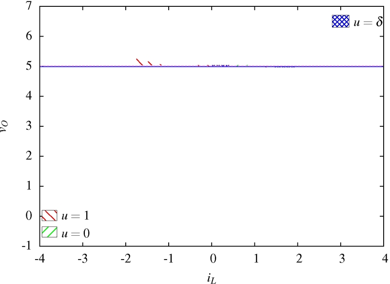
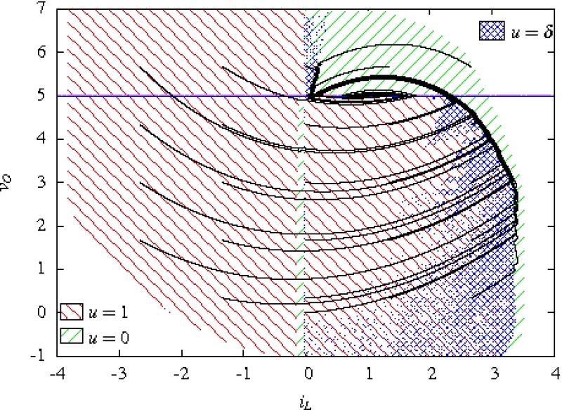
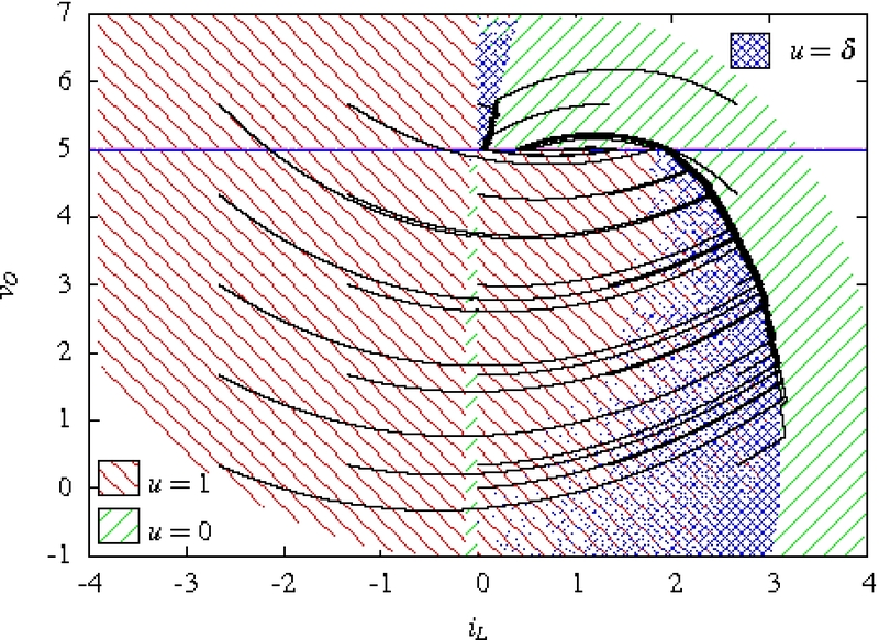
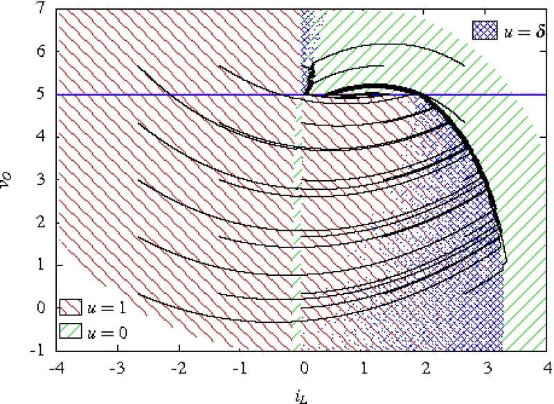
Finally, in Figs. 5–8 we show the guaranteed operational range (controlled regions, see [5] for details) of the controllers generated for the single-input buck by QKS.

Figure 5: Single-input robust buck: controlled region with $b=8$ bits

Figure 6: Single-input robust buck: controlled region with $b=9$ bits

Figure 7: Single-input robust buck: controlled region with $b=10$ bits

Figure 8: Single-input robust buck: controlled region with $b=11$ bits

6.2 Multi-input Buck

We run QKS on the multi-input buck model described in Sect. 5. Differently from Sect. 6.1, we fix the number of AD bits $b$ for QKS, namely $b=10$. On the other hand, we run multiple times QKS by varying the number $n$ of inputs for the multi-input buck. As for input voltages, we have $V_{i}=10i$ V for all $i\in[n]$. All other constants introduced in Sect. 5 are fixed as in Sect. 6.1.

Table 4: Multi-input buck DC-DC converter: control abstraction and controller synthesis results

	Control Abstraction					Controller Synthesis		Total
$n$	CPU	MEM	Arcs	MaxLoops	NoLoopsPerc	CPU	$|K|$	CPU	MEM	$\mu$
1	2.88e+04	6.41e+07	7.38e+06	1.91e+04	0.00377	1.97e+01	1.21e+04	2.88e+04	8.35e+07	Sol
2	8.94e+04	7.63e+07	1.47e+07	1.91e+04	0.00743	2.66e+01	2.52e+04	8.94e+04	8.25e+07	Sol
3	2.46e+05	9.47e+07	2.93e+07	1.90e+04	0.01162	3.66e+01	3.47e+04	2.46e+05	1.05e+08	Sol
4	6.43e+05	9.51e+07	5.84e+07	1.88e+04	0.00330	5.32e+01	4.31e+04	6.43e+05	0.00e+00	Sol

Table 5: Multi-input buck DC-DC converter: number of MILPs and time to solve them

	$n=1$			$n=2$
MILP	Num	Avg	Time	Num	Avg	Time
1	1.0e+06	2.0e-04	2.1e+02	1.0e+06	2.1e-04	2.2e+02
2	6.4e+06	1.4e-03	5.1e+03	1.3e+07	1.9e-03	1.6e+04
3	3.7e+06	8.8e-04	3.2e+03	7.4e+06	1.6e-03	1.1e+04
4	8.7e+06	1.0e-03	8.9e+03	1.7e+07	1.7e-03	2.8e+04
5	6.9e+06	6.8e-04	4.6e+03	1.4e+07	1.1e-03	1.5e+04

Table 6: Multi-input buck DC-DC converter: number of MILPs and time to solve them (continuation of Tab. 5)

	$n=3$			$n=4$
MILP	Num	Avg	Time	Num	Avg	Time
1	1.0e+06	2.1e-04	2.2e+02	1.0e+06	2.2e-04	2.3e+02
2	2.5e+07	3.0e-03	4.6e+04	5.1e+07	4.5e-03	1.2e+05
3	1.5e+07	2.2e-03	3.2e+04	2.9e+07	2.9e-03	8.6e+04
4	3.2e+07	2.4e-03	7.9e+04	6.3e+07	3.2e-03	2.0e+05
5	2.7e+07	1.6e-03	4.3e+04	5.5e+07	2.1e-03	1.1e+05

Tabs. 4, 5 and 6 show our experimental results. Columns in Tab. 4 have the following meaning. Column $n$ shows the number of inputs of the multi-input buck (see Sect. 5 for details). All other columns of Tab. 4, as well as of Tabs. 5 and 6 have the same meaning of the same columns of Tabs. 1, 2 and 3.

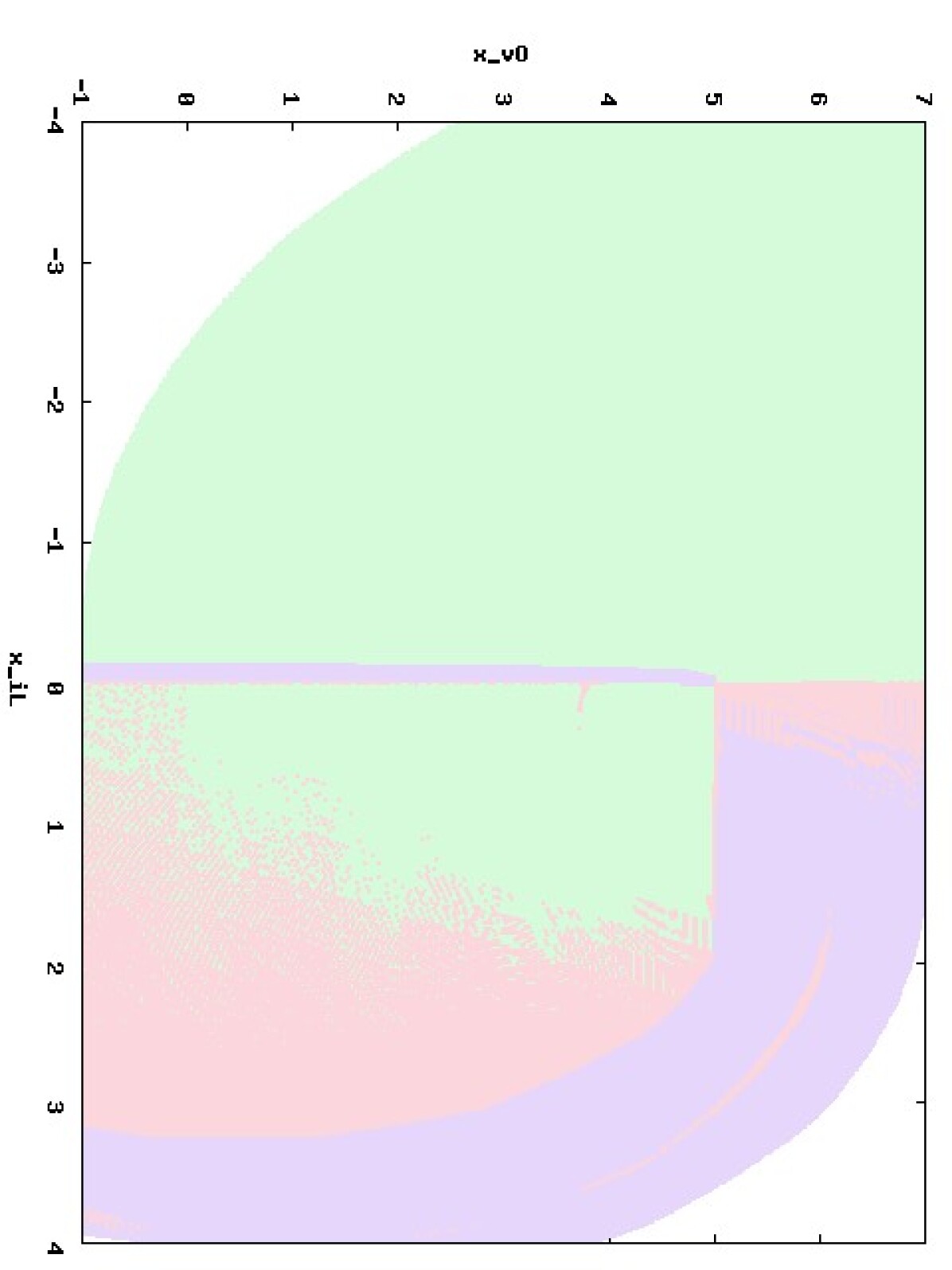
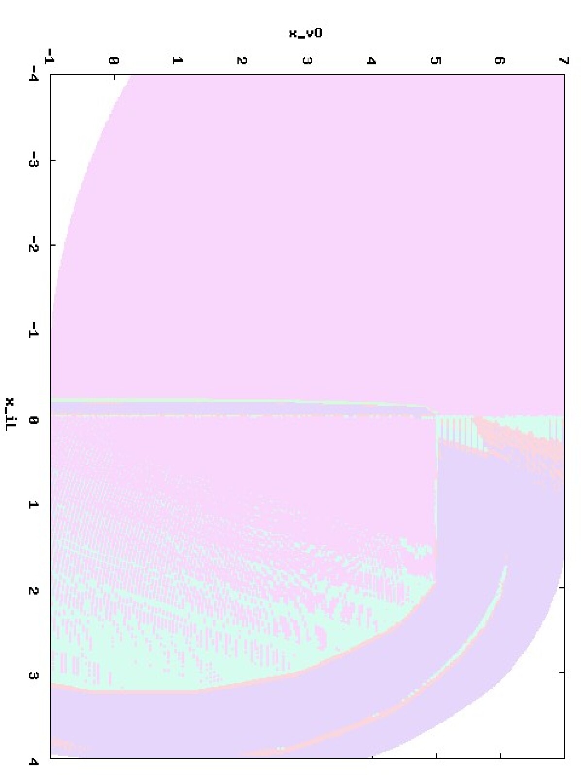
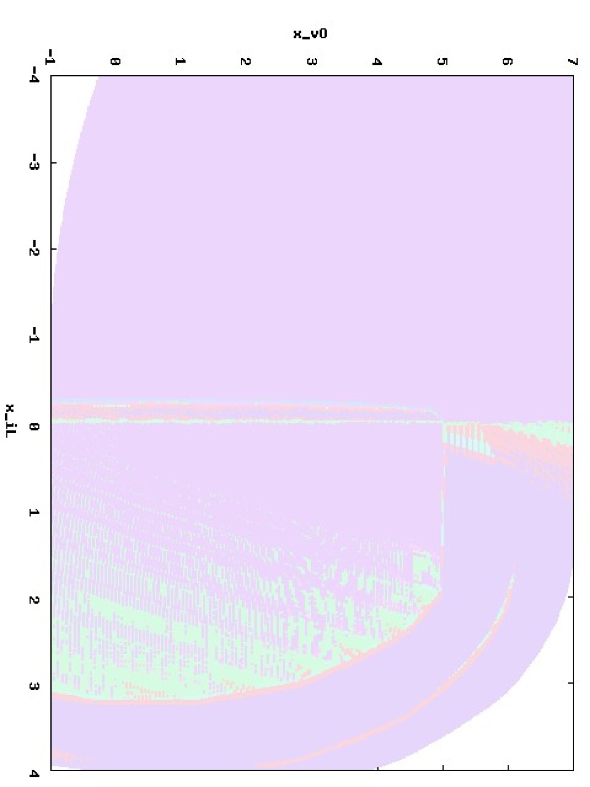
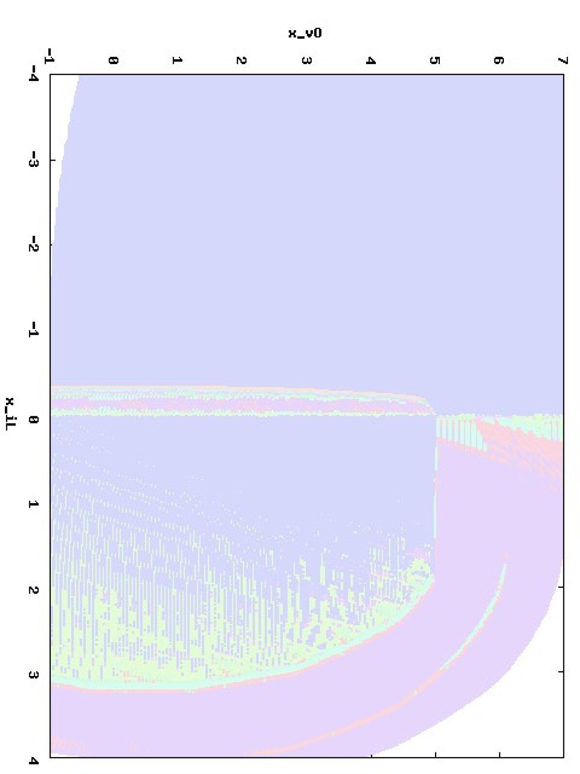
Finally, in Figs. 9–12 we show the guaranteed operational range (controlled regions, see [5] for details) of the controllers generated for the multi-input buck by QKS.

Figure 9: Multi-input buck: controlled region with $n=1$ inputs

Figure 10: Multi-input buck: controlled region with $n=2$ inputs

Figure 11: Multi-input buck: controlled region with $n=3$ inputs

Figure 12: Multi-input buck: controlled region with $n=4$ inputs

7 Conclusions

We presented experimental results on using the QKS tool [5], to support a Formal Model Based Design approach to control software. Our experiments have been carried out on two versions of the buck DC-DC converter, namely the single-input and the multi-input versions. We also showed how robust controllers may be generated for such bucks, namely by taking into account also foreseen variations on some important buck parameters such as load and input power supplies.

References

- [1] Thomas A. Henzinger, Benjamin Horowitz, Rupak Majumdar, and Howard Wong-Toi. Beyond hytech: Hybrid systems analysis using interval numerical methods. In HSCC, LNCS 1790, pages 130–144, 2000.
- [2] Thomas A. Henzinger and Joseph Sifakis. The embedded systems design challenge. In FM, LNCS 4085, pages 1–15, 2006.
- [3] W. Kim, M. S. Gupta, G.-Y. Wei, and D. M. Brooks. Enabling on-chip switching regulators for multi-core processors using current staggering. In ASGI, 2007.
- [4] Ping-Zong Lin, Chun-Fei Hsu, and Tsu-Tian Lee. Type-2 fuzzy logic controller design for buck dc-dc converters. In FUZZ, pages 365–370, 2005.
- [5] Federico Mari, Igor Melatti, Ivano Salvo, and Enrico Tronci. Synthesis of quantized feedback control software for discrete time linear hybrid systems. In CAV, LNCS 6174, pages 180–195, 2010.
- [6] M. Rodriguez, P. Fernandez-Miaja, A. Rodriguez, and J. Sebastian. A multiple-input digitally controlled buck converter for envelope tracking applications in radiofrequency power amplifiers. IEEE Trans on Pow El, 25(2):369–381, 2010.
- [7] G. Schrom, P. Hazucha, J. Hahn, D.S. Gardner, B.A. Bloechel, G. Dermer, S.G. Narendra, T. Karnik, and V. De. A 480-mhz, multi-phase interleaved buck dc-dc converter with hysteretic control. In PESC, pages 4702–4707 vol. 6. IEEE, 2004.
- [8] Wing-Chi So, C.K. Tse, and Yim-Shu Lee. Development of a fuzzy logic controller for dc/dc converters: design, computer simulation, and experimental evaluation. IEEE Trans. on Power Electronics, 11(1):24–32, 1996.
- [9] V. Yousefzadeh, A. Babazadeh, B. Ramachandran, E. Alarcon, L. Pao, and D. Maksimovic. Proximate time-optimal digital control for synchronous buck dc–dc converters. IEEE Trans. on Power Electronics, 23(4):2018–2026, 2008.