CFTP/11-011

LHC AND LEPTON FLAVOUR VIOLATION PHENOMENOLOGY IN SEESAW MODELS

J. C. ROMÃO

We review Lepton Flavour Violation (LFV) in the supersymmetric version of the seesaw mechanism (type I, II, III) and in Left-Right models. The LFV needed to explain neutrino masses and mixings is the only source of LFV and has experimental implications both in low-energy experiments where we search for the radiative decays of leptons, and at the LHC where we look at its imprint on the LFV decays of the sparticles and on slepton mass splittings. We discuss how this confrontation between high- and low-energy LFV observables may provide information about the underlying mechanism of LFV.


1 Introduction

The experimental observation of non-vanishing neutrino masses and mixings, ??\!{}^{{\bf?}} constitutes clear evidence for physics beyond the Standard Model (SM). As neutrino oscillations indisputably signal lepton flavour violation (LFV) in the neutral sector, it is only natural to expect that charged lepton flavour will also be violated in extensions of the SM where ν𝜈\nu oscillations can be naturally accommodated. The search for manifestations of charged LFV constitutes the goal of several experiments, ??\!{}^{{\bf?}} exclusively dedicated to look for signals of processes such as rare radiative as well as three-body decays and lepton conversion in muonic nuclei.

In parallel to these low-energy searches, if the high-energy Large Hadron Collider (LHC) finds signatures of supersymmetry (SUSY), it is then extremely appealing to consider SUSY models that can also accommodate neutrino oscillations. One of the most economical and elegant possibilities is perhaps to embed a seesaw mechanism in this framework, the so-called SUSY seesaw.

If the seesaw is indeed the source of both neutrino masses and leptonic mixings and accounts for low-energy LFV observables within future sensitivity reach, we show that interesting phenomena are expected to be observed at the LHC: in addition to measurable slepton mass splittings, the most striking effect will be the possible appearance of new edges in di-lepton mass distributions.

2 Models

2.1 Seesaw type I,II, III & Left-Right Model

At GUT scale the SU(5) invariant superpotentials for type I, II and III SUSY seesaw are ??\!{}^{{\bf?}}

WRHN=𝐘NINc5¯5H+12MRNcNc,subscript𝑊RHNsuperscriptsubscript𝐘𝑁Isuperscript𝑁𝑐¯5subscript5𝐻12subscript𝑀𝑅superscript𝑁𝑐superscript𝑁𝑐W_{\rm RHN}={\bf Y}_{N}^{\rm I}\ N^{c}\ \overline{5}\cdot 5_{H}+\frac{1}{2}\ M_{R}\ N^{c}N^{c}\ , (1)
W15H=subscript𝑊15Habsent\displaystyle W_{\rm 15H}= 12𝐘NII5¯155¯+12λ15¯H155¯H+12λ25H15¯5H+𝐘5105¯5¯H12superscriptsubscript𝐘𝑁II¯515¯512subscript𝜆1subscript¯5𝐻15subscript¯5𝐻12subscript𝜆2subscript5𝐻¯15subscript5𝐻subscript𝐘510¯5subscript¯5𝐻\displaystyle\frac{1}{\sqrt{2}}{\bf Y}_{N}^{\rm II}\ {\bar{5}}\cdot 15\cdot{\bar{5}}+\frac{1}{\sqrt{2}}\lambda_{1}{\bar{5}}_{H}\cdot 15\cdot{\bar{5}}_{H}+\frac{1}{\sqrt{2}}\lambda_{2}5_{H}\cdot\overline{15}\cdot 5_{H}+{\bf Y}_{5}10\cdot{\bar{5}}\cdot{\bar{5}}_{H}
+𝐘1010105H+M151515¯+M55¯H5H,subscript𝐘101010subscript5𝐻subscript𝑀1515¯15subscript𝑀5subscript¯5𝐻subscript5𝐻\displaystyle+{\bf Y}_{10}10\cdot 10\cdot 5_{H}+M_{15}15\cdot\overline{15}+M_{5}{\bar{5}}_{H}\cdot 5_{H}\ , (2)
W24H=subscript𝑊24Habsent\displaystyle W_{\rm 24H}= 25¯MY510M5¯H1410MY1010M5H+5H24MYNIII5¯M+1224MM2424M.2subscript¯5𝑀superscript𝑌5subscript10𝑀subscript¯5𝐻14subscript10𝑀superscript𝑌10subscript10𝑀subscript5𝐻subscript5𝐻subscript24𝑀subscriptsuperscript𝑌𝐼𝐼𝐼𝑁subscript¯5𝑀12subscript24𝑀subscript𝑀24subscript24𝑀\displaystyle\sqrt{2}\,{\bar{5}}_{M}Y^{5}10_{M}{\bar{5}}_{H}-\frac{1}{4}10_{M}Y^{10}10_{M}5_{H}+5_{H}24_{M}Y^{III}_{N}{\bar{5}}_{M}+\frac{1}{2}24_{M}M_{24}24_{M}\ . (3)
type-I type-II type-III
\psfrag{nL}{$\nu_{L}$}\psfrag{nR}{$N^{c}$}\psfrag{MR}{$M_{R}$}\psfrag{f}{\hskip-5.69054pt$\left\langle H_{u}\right\rangle$}\includegraphics[clip,height=85.35826pt]{typeI.eps} \psfrag{nL}{$\nu_{L}$}\psfrag{nR}{$\nu_{R}$}\psfrag{MR}{$M_{R}$}\psfrag{f}{\hskip-5.69054pt$\left\langle H_{u}\right\rangle$}\psfrag{D}{$T^{0}$}\psfrag{m}{$\mu$}\psfrag{YD}{$Y_{\nu}^{II}$}\includegraphics[height=85.35826pt]{typeII-Moriond.eps} \psfrag{nL}{$\nu_{L}$}\psfrag{nR}{$W_{M}$}\psfrag{MR}{$M_{W_{M}}$}\psfrag{f}{\hskip-5.69054pt$\left\langle H_{u}\right\rangle$}\includegraphics[clip,height=85.35826pt]{typeI.eps}
Figure 1: Seesaw types

The exchange of the singlet Ncsuperscript𝑁𝑐N^{c} in type I, of the scalar triplet T𝑇T in type II and of both the fermionic triplet WMsubscript𝑊𝑀W_{M} and fermionic singlet BMsubscript𝐵𝑀B_{M} in type III lead, through the diagrams of Fig. 1 to the well known effective neutrino mass matrix formulas,

meffI=(vYν)MR1(vYν)T,meffII=v2μYνIIMT2,meffIII=(vYνIII)MWM1(vYνIII)T.formulae-sequencesuperscriptsubscript𝑚effI𝑣subscript𝑌𝜈superscriptsubscript𝑀𝑅1superscript𝑣subscript𝑌𝜈𝑇formulae-sequencesuperscriptsubscript𝑚effIIsuperscript𝑣2𝜇superscriptsubscript𝑌𝜈IIsubscriptsuperscript𝑀2𝑇superscriptsubscript𝑚effIII𝑣superscriptsubscript𝑌𝜈IIIsuperscriptsubscript𝑀subscript𝑊𝑀1superscript𝑣superscriptsubscript𝑌𝜈III𝑇m_{\rm eff}^{\rm I}=-(vY_{\nu})M_{R}^{-1}(vY_{\nu})^{T},\quad m_{\rm eff}^{\rm II}=\frac{v^{2}\mu Y_{\nu}^{\rm II}}{M^{2}_{T}},\quad m_{\rm eff}^{\rm III}=-(vY_{\nu}^{\rm III})M_{W_{M}}^{-1}(vY_{\nu}^{\rm III})^{T}\ . (4)

We have also studied ??\!{}^{{\bf?}} a SUSY seesaw in which the breaking from SU(5)𝑆𝑈5SU(5) to the SM gauge group is done in two steps, first to a Left-Right (LR) symmetric model, SU(3)c×SU(2)L×SU(2)R×U(1)BL𝑆𝑈subscript3𝑐𝑆𝑈subscript2𝐿𝑆𝑈subscript2𝑅𝑈subscript1𝐵𝐿SU(3)_{c}\times SU(2)_{L}\times SU(2)_{R}\times U(1)_{B-L} at scale vRsubscript𝑣𝑅v_{R}, and then with the BL𝐵𝐿B-L broken at a lower scale vBLsubscript𝑣𝐵𝐿v_{B-L}. For neutrino physics, as well as for the LFV, the relevant part of the superpotential is,

𝒲LR=YLLΦLcfcLcΔcLc+,superscript𝒲𝐿𝑅subscript𝑌𝐿𝐿Φsuperscript𝐿𝑐subscript𝑓𝑐superscript𝐿𝑐superscriptΔ𝑐superscript𝐿𝑐\mathcal{W}^{LR}=Y_{L}L\Phi L^{c}-f_{c}L^{c}\Delta^{c}L^{c}+\cdots\ , (5)

where YLsubscript𝑌𝐿Y_{L} and fcsubscript𝑓𝑐f_{c} complex 3×3333\times 3 matrices. After the BL𝐵𝐿B-L breaking we have,

=HuνL¯YνIνR12νRTC1(fcvBL)νR+,subscript𝐻𝑢¯subscript𝜈𝐿superscriptsubscript𝑌𝜈Isubscript𝜈𝑅12superscriptsubscript𝜈𝑅𝑇superscript𝐶1subscript𝑓𝑐subscript𝑣𝐵𝐿subscript𝜈𝑅\mathcal{L}=H_{u}\,\overline{\nu_{L}}\,Y_{\nu}^{\rm I}\,\nu_{R}-\frac{1}{2}\nu_{R}^{T}\,C^{-1}\,(f_{c}v_{BL})\,\nu_{R}+\cdots\ , (6)

leading to an effective neutrino mass matrix of the type I form,

meffLR=(vYν)(fcvBL)1(vYν)T.superscriptsubscript𝑚effLR𝑣subscript𝑌𝜈superscriptsubscript𝑓𝑐subscript𝑣𝐵𝐿1superscript𝑣subscript𝑌𝜈𝑇m_{\rm eff}^{\rm LR}=-(vY_{\nu})(f_{c}v_{BL})^{-1}(vY_{\nu})^{T}\ . (7)

The important point here is that, as we have two complex matrices, we can have different types of neutrino fits. We studied two limiting situations, the so-called Yνsubscript𝑌𝜈Y_{\nu} fit where fc=𝟙subscript𝑓𝑐1f_{c}=\mathds{1} (Yνsubscript𝑌𝜈Y_{\nu} arbitrary), and the f𝑓f fit where Yν=𝟙subscript𝑌𝜈1Y_{\nu}=\mathds{1} (fcsubscript𝑓𝑐f_{c} arbitrary). These will leave different imprints on the LFV through their RGE running.

2.2 LFV in the Models

Starting with universal minimal supergravity inspired (mSUGRA) boundary conditions at MGUTsubscript𝑀GUTM_{\rm GUT}, the off-diagonal entries in Yνsuperscript𝑌𝜈Y^{\nu} will induce the LFV on the slepton mass matrices through RGE effects. For type I, II and III we have

ΔmL,ij2ak8π2(3m02+A02)(YNk,LYNk)ij,L=ln(MGUTMN)formulae-sequencesimilar-to-or-equalsΔsubscriptsuperscript𝑚2𝐿𝑖𝑗subscript𝑎𝑘8superscript𝜋23subscriptsuperscript𝑚20subscriptsuperscript𝐴20subscriptsubscriptsuperscript𝑌𝑘𝑁𝐿subscriptsuperscript𝑌𝑘𝑁𝑖𝑗𝐿subscript𝑀GUTsubscript𝑀N\displaystyle\Delta m^{2}_{L,ij}\simeq-\frac{a_{k}}{8\pi^{2}}\left(3m^{2}_{0}+A^{2}_{0}\right)\left(Y^{k,\dagger}_{N}LY^{k}_{N}\right)_{ij},\quad L=\ln(\frac{M_{\rm GUT}}{M_{\rm N}}) (8)
ΔmE,ij20aI=1,aII=6andaIII=95,formulae-sequencesimilar-to-or-equalsΔsubscriptsuperscript𝑚2𝐸𝑖𝑗0subscript𝑎I1subscript𝑎II6andsubscript𝑎III95\displaystyle\Delta m^{2}_{E,ij}\simeq 0\hskip 56.9055pta_{\rm I}=1\,\,,\,\,a_{\rm II}=6\,\,\mathrm{and}\,\,\,a_{\rm III}=\frac{9}{5}\ , (9)

while for the LR model we have two situations. From MGUTsubscript𝑀GUTM_{\rm GUT} to vRsubscript𝑣𝑅v_{R},

ΔmL2Δsuperscriptsubscript𝑚𝐿2\displaystyle\Delta m_{L}^{2} 14π2(3ff+YL(k)YL(k))(3m02+A02)ln(MGUTvR)similar-to-or-equalsabsent14superscript𝜋23𝑓superscript𝑓superscriptsubscript𝑌𝐿𝑘superscriptsubscript𝑌𝐿𝑘3superscriptsubscript𝑚02superscriptsubscript𝐴02subscript𝑀GUTsubscript𝑣𝑅\displaystyle\simeq-\frac{1}{4\pi^{2}}\left(3ff^{\dagger}+Y_{L}^{(k)}Y_{L}^{(k)\>\dagger}\right)(3m_{0}^{2}+A_{0}^{2})\ln\left(\frac{M_{\rm GUT}}{v_{R}}\right) (10)
ΔmE2Δsuperscriptsubscript𝑚𝐸2\displaystyle\Delta m_{E}^{2} 14π2(3ff+YL(k)YL(k))(3m02+A02)ln(MGUTvR),similar-to-or-equalsabsent14superscript𝜋23superscript𝑓𝑓superscriptsubscript𝑌𝐿𝑘superscriptsubscript𝑌𝐿𝑘3superscriptsubscript𝑚02superscriptsubscript𝐴02subscript𝑀GUTsubscript𝑣𝑅\displaystyle\simeq-\frac{1}{4\pi^{2}}\left(3f^{\dagger}f+Y_{L}^{(k)\>\dagger}Y_{L}^{(k)}\right)(3m_{0}^{2}+A_{0}^{2})\ln\left(\frac{M_{\rm GUT}}{v_{R}}\right)\ , (11)

while from vRsubscript𝑣𝑅v_{R} to vBLsubscript𝑣𝐵𝐿v_{BL},

ΔmL2Δsuperscriptsubscript𝑚𝐿2\displaystyle\Delta m_{L}^{2} 18π2YνYν(mL2|vR+Ae2|vR)ln(vRvBL),ΔmE20.formulae-sequencesimilar-to-or-equalsabsent18superscript𝜋2subscript𝑌𝜈superscriptsubscript𝑌𝜈evaluated-atsuperscriptsubscript𝑚𝐿2subscript𝑣𝑅evaluated-atsuperscriptsubscript𝐴𝑒2subscript𝑣𝑅subscript𝑣𝑅subscript𝑣𝐵𝐿similar-to-or-equalsΔsuperscriptsubscript𝑚𝐸20\displaystyle\simeq-\frac{1}{8\pi^{2}}Y_{\nu}Y_{\nu}^{\dagger}\left(m_{L}^{2}|_{v_{R}}+A_{e}^{2}|_{v_{R}}\right)\ln\left(\frac{v_{R}}{v_{BL}}\right),\quad\Delta m_{E}^{2}\simeq 0\ . (12)

Therefore, the choice of the different neutrino fits will have implications on the lepton flavour violation observables. The low energy LFV processes are described by an effective Lagrangian,

eff=emli2l¯iσμνFμν(ALijPL+ARijPR)lj+h.c.formulae-sequencesubscript𝑒𝑓𝑓𝑒subscript𝑚subscript𝑙𝑖2subscript¯𝑙𝑖subscript𝜎𝜇𝜈superscript𝐹𝜇𝜈superscriptsubscript𝐴𝐿𝑖𝑗subscript𝑃𝐿superscriptsubscript𝐴𝑅𝑖𝑗subscript𝑃𝑅subscript𝑙𝑗𝑐\mathcal{L}_{eff}=e\frac{m_{l_{i}}}{2}\ \bar{l}_{i}\sigma_{\mu\nu}F^{\mu\nu}(A_{L}^{ij}P_{L}+A_{R}^{ij}P_{R})l_{j}+h.c. (13)

For seesaw models,

ALij(ΔmL2)ijmSUSY4,ARij(ΔmE2)ijmSUSY4.formulae-sequencesimilar-tosuperscriptsubscript𝐴𝐿𝑖𝑗subscriptΔsuperscriptsubscript𝑚𝐿2𝑖𝑗superscriptsubscript𝑚SUSY4similar-tosuperscriptsubscript𝐴𝑅𝑖𝑗subscriptΔsuperscriptsubscript𝑚𝐸2𝑖𝑗superscriptsubscript𝑚SUSY4A_{L}^{ij}\sim\frac{(\Delta m_{L}^{2})_{ij}}{m_{\rm SUSY}^{4}},\quad A_{R}^{ij}\sim\frac{(\Delta m_{E}^{2})_{ij}}{m_{\rm SUSY}^{4}}\ . (14)

This implies that for type I, II and II we have only AL0subscript𝐴𝐿0A_{L}\not=0, while for the LR model we can have both, ALsubscript𝐴𝐿A_{L} and ARsubscript𝐴𝑅A_{R}. This implies that if MEG ??\!{}^{{\bf?}} finds evidence for the decay μ+e+γsuperscript𝜇superscript𝑒𝛾\mu^{+}\to e^{+}\gamma, then we can distinguish among the models by looking at the positron polarization asymmetry,

𝒜(μ+e+γ)=|AL|2|AR|2|AL|2+|AR|2{=1type-I-II-III1LR.𝒜superscript𝜇superscript𝑒𝛾superscriptsubscript𝐴𝐿2superscriptsubscript𝐴𝑅2superscriptsubscript𝐴𝐿2superscriptsubscript𝐴𝑅2casesabsent1type-I-II-IIIabsent1LR\mathcal{A}(\mu^{+}\to e^{+}\gamma)=\frac{|A_{L}|^{2}-|A_{R}|^{2}}{|A_{L}|^{2}+|A_{R}|^{2}}\ \left\{\begin{array}[]{cl}=1&\text{type-I-II-III}\\ \not=1&\text{LR}\end{array}\right.\quad. (15)

3 Results

For all the models we have studied ??\!{}^{{\bf?}},,{}^{\!,\,}??\!{}^{{\bf?}},,{}^{\!,\,}??\!{}^{{\bf?}} the different low- and high-energy LFV observables. The numerical analysis was done using the public code SPheno, ??\!{}^{{\bf?}} that includes the 2-loop RGEs calculated with the public code SARAH. ??\!{}^{{\bf?}}

3.1 Low-Energy Observables

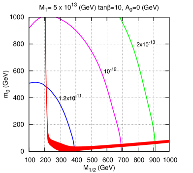
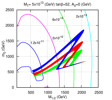
The present bounds on low-energy LFV observables and dark matter abundance already constrain the parameter space of the models. As an example we give in Fig. 2 the type II case. On the left panel we show the allowed regions for dark matter abundance (within 3σ𝜎\sigma of the WMAP ??\!{}^{{\bf?}} observation). A scan was performed in the M1/2m0subscript𝑀12subscript𝑚0M_{1/2}-m_{0} plane, the other cMSSM parameters being taken as A0=0subscript𝐴00A_{0}=0, tanβ=10𝛽10\tan\beta=10, μ>0𝜇0\mu>0. The seesaw scale was fixed at MT=5×10¹³subscript𝑀𝑇5superscript1013M_{T}=5\times 10^{13} GeV. Superimposed are the contours for BR(μeγ𝜇𝑒𝛾\mu\to e\gamma). We see that for these input parameters only a small part of the parameter space remains viable after imposing the LFV and dark matter constrains. Once MEG gets to the sensitivity of 1013superscript101310^{-13}, most of the parameter space will be excluded if no signal is found. On the right panel of Fig. 2 we show a similar plot, now in the so-called Higgs funnel region obtained for tanβ=52𝛽52\tan\beta=52, the other parameters as before. The variation with the top mass is shown: mtop=169.1subscript𝑚𝑡𝑜𝑝169.1m_{top}=169.1 GeV (blue), 171.2171.2171.2 GeV (red), 173.3173.3173.3 GeV (green).

Refer to caption Refer to caption
Figure 2: Dark matter allowed regions and BR(μeγ𝜇𝑒𝛾\mu\to e\gamma) contours for type II,

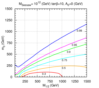
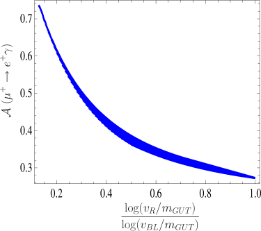
As another example we consider the e+superscript𝑒e^{+} asymmetry defined in Eq. (15) in the LR model ??\!{}^{{\bf?}}. On the left panel of Fig. 3 we show the contours for 𝒜𝒜\mathcal{A} in the M1/2m0subscript𝑀12subscript𝑚0M_{1/2}-m_{0} plane. The cMSSM parameters were taken as those of the SPS3 point, m0=90subscript𝑚090m_{0}=90 GeV, M1/2=400subscript𝑀12400M_{1/2}=400 GeV, A0=0subscript𝐴00A_{0}=0 GeV, tanβ=10𝛽10\tan\beta=10 and μ>0𝜇0\mu>0. We take MSeesaw=1012subscript𝑀Seesawsuperscript1012M_{\rm Seesaw}=10^{12} GeV, while the LR breaking scales were vBL=1015subscript𝑣𝐵𝐿superscript1015v_{BL}=10^{15} GeV, vR[1014,1015]subscript𝑣𝑅superscript1014superscript1015v_{R}\in[10^{14},10^{15}] GeV and Yνsubscript𝑌𝜈Y_{\nu} fit was chosen. On the right panel we show, for the same parameters, the correlation between the asymmetry and the breaking scales. If MEG measures 𝒜<1𝒜1\mathcal{A}<1, we can have an handle on the scales vR,vBLsubscript𝑣𝑅subscript𝑣𝐵𝐿v_{R},v_{BL} and test the LR model.

Refer to caption
Refer to caption
Figure 3: Positron asymmetry in the Left-Right model.

3.2 LHC Observables

At LHC we look at di-lepton invariant mass distributions from χ20~L,Riχ10superscriptsubscript𝜒20subscriptsuperscript~𝑖𝐿𝑅subscriptsuperscriptsubscript𝜒10\chi_{2}^{0}\rightarrow\tilde{\ell}^{i}_{L,R}\ell_{\rightarrow}\chi_{1}^{0}\ell\ell decays, that can be measured with a precision of 0.1%percent0.10.1\%, ??\!{}^{{\bf?}} for on-shell sleptons and isolated leptons with large pT>10subscript𝑝𝑇10p_{T}>10 GeV. From this we can infer the slepton mass splittings,

Δm~m~(~i,~j)=|m~im~j|<m~i,j>@LHC:Δm/m~(e~L,μ~L)𝒪(0.1%)Δm/m~(μ~L,τ~L)𝒪(1%).:Δsubscript𝑚~subscript𝑚~subscript~𝑖subscript~𝑗subscript𝑚subscript~𝑖subscript𝑚subscript~𝑗expectationsubscript𝑚subscript~𝑖𝑗@LHCsimilar-toΔ𝑚subscript𝑚~subscript~𝑒𝐿subscript~𝜇𝐿𝒪percent0.1similar-toΔ𝑚subscript𝑚~subscript~𝜇𝐿subscript~𝜏𝐿𝒪percent1\frac{\Delta m_{\tilde{\ell}}}{m_{\tilde{\ell}}}(\tilde{\ell}_{i},\tilde{\ell}_{j})\,=\,\frac{|m_{\tilde{\ell}_{i}}-m_{\tilde{\ell}_{j}}|}{<m_{\tilde{\ell}_{i,j}}>}\quad@\text{LHC}:\begin{array}[]{l}\Delta m/m_{\tilde{\ell}}(\tilde{e}_{L},\tilde{\mu}_{L})\sim\mathcal{O}(0.1\%)\\ \Delta m/m_{\tilde{\ell}}(\tilde{\mu}_{L},\tilde{\tau}_{L})\sim\mathcal{O}(1\%)\ .\end{array} (16)

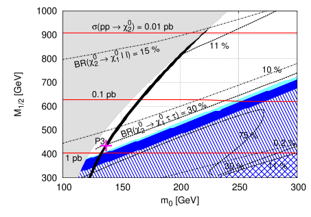
We start our analysis by identifying what we call a standard window. This is defined by the requirement of having on-shell sleptons decaying with isolated leptons with large pT>10subscript𝑝𝑇10p_{T}>10 GeV. We also require large χ20superscriptsubscript𝜒20\chi_{2}^{0} production, a sizable BR(χ20χ10superscriptsubscript𝜒20superscriptsubscript𝜒10\chi_{2}^{0}\rightarrow\chi_{1}^{0}\ell\ell) and, if possible, the correct abundance of dark matter, Ωh2Ωsuperscript2\Omega h^{2}. This is shown on the left panel of Fig. 4,
Refer to caption
Point m0subscript𝑚0m_{0} M1/2subscript𝑀12M_{1/2} A0subscript𝐴0A_{0} tanβ𝛽\tan\beta
(GeV) (GeV) (TeV)
P1 110 528 0 10
P2 110 471 1 10
P3 137 435 -1 10
P4 490 1161 0 40
P5-HM1 180 850 0 10
P6-SU1 70 350 0 10
Figure 4: Standard window (see text) and benchmark points used in the analysis.

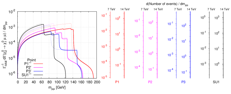
where the white region fulfills all the requirements (the correct dark matter abundance corresponds to the black line inside the region). To carry out our analysis we chose the cMSSM study points shown in the right panel of Fig. 4 and then varied the seesaw parameters. In the cMSSM we get double-triangular distributions corresponding to intermediate μ~Lsubscript~𝜇𝐿\tilde{\mu}_{L} and μ~Rsubscript~𝜇𝑅\tilde{\mu}_{R} in χ20χ10μμsuperscriptsubscript𝜒20superscriptsubscript𝜒10𝜇𝜇\chi_{2}^{0}\!\rightarrow\!\chi_{1}^{0}\mu\mu, with superimposed ~L,Rsubscript~𝐿𝑅\tilde{\ell}_{L,R} edges for mμμsubscript𝑚𝜇𝜇m_{\mu\mu} and meesubscript𝑚𝑒𝑒m_{ee} because of “degenerate” μ~,e~~𝜇~𝑒\tilde{\mu},\tilde{e}. In Fig. 5 we show the di-muon invariant distribution, and number of expected events, for the case of SUSY type I seesaw, for the following choice of seesaw parameters: MNsubscript𝑀𝑁M_{N}={1010,5×1010,5×1013}superscript10105superscript10105superscript1013\{10^{10},5\times 10^{10},5\times 10^{13}\} GeV (P2, P3) and MNsubscript𝑀𝑁M_{N}={1010,5×1012,1015}superscript10105superscript1012superscript1015\{10^{10},5\times 10^{12},10^{15}\} GeV (P1′′′, SU1′′′), always with θ13=0.1subscript𝜃13superscript0.1\theta_{13}=0.1^{\circ}.

Refer to caption
Figure 5: Di-muon invariant mass distribution for the SUSY seesaw for the benchmark points defined in Fig. 4.

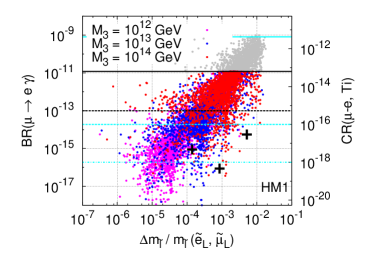
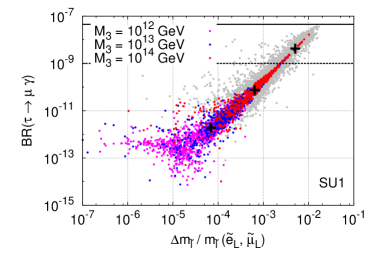
We get displaced mμμsubscript𝑚𝜇𝜇m_{\mu\mu} and meesubscript𝑚𝑒𝑒m_{ee} edges (Lsubscript𝐿\ell_{L}) which give sizable mass splittings Δm~m~(e~L,μ~L)Δsubscript𝑚~subscript𝑚~subscript~𝑒𝐿subscript~𝜇𝐿\frac{\Delta m_{\tilde{\ell}}}{m_{\tilde{\ell}}}(\tilde{e}_{L},\tilde{\mu}_{L}). We also find the appearance of a new edge in mμμsubscript𝑚𝜇𝜇m_{\mu\mu} corresponding to an intermediate τ~2subscript~𝜏2\tilde{\tau}_{2}. These mass splittings are correlated with the low-energy observables as we show in Fig. 6. On the left panel we show the correlation for BR(μeγ𝜇𝑒𝛾\mu\to e\gamma) for the CMS benchmark point HM1 (m0=180subscript𝑚0180m_{0}=180 GeV, M1/2=800subscript𝑀12800M_{1/2}=800 GeV, A0=0subscript𝐴00A_{0}=0 GeV, tanβ=10𝛽10\tan\beta=10 and μ>0𝜇0\mu>0)

Refer to caption Refer to caption
Figure 6: Correlation between low-energy and LHC observables for the benchmark points HM1 and SU1.

while on the right panel we show the correlation for BR(τμγ𝜏𝜇𝛾\tau\to\mu\gamma) for the ATLAS benchmark point SU1 (m0=70subscript𝑚070m_{0}=70 GeV, M1/2=350subscript𝑀12350M_{1/2}=350 GeV, A0=0subscript𝐴00A_{0}=0 GeV, tanβ=10𝛽10\tan\beta=10 and μ>0𝜇0\mu>0). In these plots we performed a scan over the SUSY seesaw parameters, with MN3=1012,13,14subscript𝑀subscript𝑁3superscript10121314M_{N_{3}}=10^{12,13,14} GeV, θ13=0.1subscript𝜃13superscript0.1\theta_{13}=0.1^{\circ}.

We conclude that if SUSY is discovered with a spectrum similar to HM1 or SU1 and a type-I seesaw is at work, then the LFV observables will be within experimental reach at LHC, while BR(μeγ𝜇𝑒𝛾\mu\rightarrow e\gamma) and BR(τeγ𝜏𝑒𝛾\tau\rightarrow e\gamma) will be within the reach of MEG and SuperB, respectively.

4 Conclusions

In SUSY seesaw models the neutrino Yukawa couplings, Yνsubscript𝑌𝜈Y_{\nu}, acts as the only source of LFV, implying a correlation between low- and high-energy LFV observables. We have performed a study of these correlations in the so-called SUSY seesaws type I, II and III, as well as in a seesaw model that is Left-Right symmetric below the GUT scale.

If SUSY seesaw is to account for neutrino masses and mixings then we will have slepton mass splittings within LHC sensitivity, with the possible observation of new edges in the di-lepton invariant mass distributions. In most cases a clear correlation can be established between low- and high-energy LFV observables (e.g. BR vs Δm~Δsubscript𝑚~\Delta m_{\tilde{\ell}}) due to their unique source.

The experimental data that will be available soon, both from the high- and low-energy experiments, will either substantiate the seesaw hypothesis, or disfavour the SUSY seesaw as the (only) source of flavour violation.

Acknowledgments

This work has been done partly under the EU Network grant UNILHC PITN-GA-2009-237920 and from Fundação para a Ciência e a Tecnologia grants CFTP-FCT UNIT 777, PTDC/FIS/102120/2008, CERN/FP/109305/2009.

References

References

  • [1] For a recent review see T. Schwetz, M. Tortola, J. W. F. Valle, [arXiv:1103.0734 [hep-ph]].
  • [2] For a comprehensive list see Ref. ??\!{}^{{\bf?}}.
  • [3] M. Hirsch, J. W. F. Valle, W. Porod, J. C. Romao and A. Villanova del Moral, Phys. Rev. D 78 (2008) 013006; J. N. Esteves, J. C. Romao, A. Villanova del Moral, M. Hirsch, J. W. F. Valle and W. Porod, JHEP 0905, 003 (2009); J. N. Esteves, J. C. Romao, M. Hirsch, F. Staub and W. Porod, Phys. Rev. D 83 (2011) 013003.
  • [4] J. N. Esteves, J. C. Romao, M. Hirsch, A. Vicente, W. Porod, F. Staub, JHEP 1012 (2010) 077.
  • [5] A. Abada, A. J. R. Figueiredo, J. C. Romao and A. M. Teixeira, JHEP 1010 (2010) 104; ibidem [arXiv:1104.3962 [hep-ph]].
  • [6] W. Porod, Comput. Phys. Commun.  153, (2003) 275.
  • [7] F. Staub, Comput. Phys. Commun. 181 (2010) 1077-1086.
  • [8] D. Larson et al., Astrophys.  J. Suppl.  192 (2011) 16.
  • [9] F. E. Paige, ”Determining SUSY particle masses at LHC”, arXiv:hep-ph/9609373; I. Hinchliffe, F. E. Paige, M. D. Shapiro, J. Soderqvist and W. Yao, Phys. Rev. D 55 (1997) 5520; H. Bachacou, I. Hinchliffe and F. E. Paige, Phys. Rev. D 62 (2000) 015009.