Kernel Belief Propagation
Le Song,1 Arthur Gretton,1,2 Danny Bickson,1 Yucheng Low,1 Carlos Guestrin1 1 School of Computer Science, CMU; 2Gatsby Computational Neuroscience Unit & MPI for Biological Cybernetics
Abstract
We propose a nonparametric generalization of belief propagation, Kernel Belief Propagation (KBP), for pairwise Markov random fields. Messages are represented as functions in a reproducing kernel Hilbert space (RKHS), and message updates are simple linear operations in the RKHS. KBP makes none of the assumptions commonly required in classical BP algorithms: the variables need not arise from a finite domain or a Gaussian distribution, nor must their relations take any particular parametric form. Rather, the relations between variables are represented implicitly, and are learned nonparametrically from training data. KBP has the advantage that it may be used on any domain where kernels are defined (, strings, groups), even where explicit parametric models are not known, or closed form expressions for the BP updates do not exist. The computational cost of message updates in KBP is polynomial in the training data size. We also propose a constant time approximate message update procedure by representing messages using a small number of basis functions. In experiments, we apply KBP to image denoising, depth prediction from still images, and protein configuration prediction: KBP is faster than competing classical and nonparametric approaches (by orders of magnitude, in some cases), while providing significantly more accurate results.
1 Introduction
Belief propagation is an inference algorithm for graphical models that has been widely and successfully applied in a great variety of domains, including vision (Sudderth et al., 2003), protein folding (Yanover & Weiss, 2002), and turbo decoding (McEliece et al., 1998). In these applications, the variables are usually assumed either to be finite dimensional, or in continuous cases, to have a Gaussian distribution (Weiss & Freeman, 2001). In many applications of graphical models, however, the variables of interest are naturally specified by continuous, non-Gaussian distributions. For example, in constructing depth maps from 2D images, the depth is both continuous valued and has a multimodal distribution. Likewise, in protein folding, angles are modeled as continuous valued random variables, and are predicted from amino acid sequences. In general, multimodalities, skewness, and other non-Gaussian statistical features are present in a great many real-world problems. The corresponding inference procedures for parametric models typically involve integrals for which no closed form solutions exist, and are without computationally tractable exact message updates. Worse still, parametric models for the relations between the variables may not even be known, or may be prohibitively complex.
Our first contribution in this paper is a novel generalization of belief propagation for pairwise Markov random fields, Kernel BP, based on a reproducing kernel Hilbert space (RKHS) representation of the relations between random variables. This extends earlier work of Song et al. (2010) on inference for trees to the case of graphs with loops. The algorithm consists of two parts, both nonparametric: first, we learn RKHS representations of the relations between variables directly from training data, which removes the need for an explicit parametric model. Second, we propose a belief propagation algorithm for inference based on these learned relations, where each update is a linear operation in the RKHS (although the relations themselves may be highly nonlinear in the original space of the variables). Our approach applies not only to continuous-valued non-Gaussian variables, but also generalizes to strings and graphs (Schölkopf et al., 2004), groups (Fukumizu et al., 2009), compact manifolds (Wendland, 2005, Chapter 17), and other domains on which kernels may be defined.
A number of alternative approaches have been developed to perform inference in the continuous-valued non-Gaussian setting. Sudderth et al. (2003) proposed an approximate belief propagation algorithm for pairwise Markov random fields, where the parametric forms of the node and edge potentials are supplied in advance, and the messages are approximated as mixtures of Gaussians: we refer to this approach as Gaussian Mixture BP (this method was introduced as “nonparametric BP”, but it is in fact a Gaussian mixture approach). Instead of mixtures of Gaussians, Ihler & McAllester (2009) used particles to approximate the messages, resulting in the Particle BP algorithm. Both Gaussian mixture BP and particle BP assume the potentials to be pre-specified by the user: the methods described are purely approximate message update procedures, and do not learn the model from training data. By contrast, kernel BP learns the model, is computationally tractable even before approximations are made, and leads to an entirely different message update formula than the Gaussian Mixture and Particle representations.
A direct implementation of kernel BP has a reasonable computational cost: each message update costs when computed exactly, where is the number of training examples and is the maximum degree of a node in the graphical model. For massive data sets and numbers of nodes, as occur in image processing, this cost might still be expensive. Our second contribution is a novel constant time approximate message update procedure, where we express the messages in terms of a small number of representative RKHS basis functions learned from training data. Following an initialization cost linear in , the cost per message update is decreased to , independent of the number of training points . Even without these approximate constant time updates, kernel BP is substantially faster than Gaussian mixture BP and particle BP. Indeed, an exact implementation of Gaussian mixture BP would have an exponentially increasing computational and storage cost with number of iterations. In practice, both Gaussian mixture and particle BP require a Monte Carlo resampling procedure at every node of the graphical model.
Our third contribution is a thorough evaluation of kernel BP against other nonparametric BP approaches. We apply both kernel BP and competing approaches to an image denoising problem, depth prediction from still images, protein configuration prediction, and paper topic inference from citation networks: these are all large-scale problems, with continuous-valued or structured random variables having complex underlying probability distributions. In all cases, kernel BP performs outstandingly, being orders of magnitude faster than both Gaussian mixture BP and particle BP, and returning more accurate results.
2 Markov Random Fields And Belief Propagation
We begin with a short introduction to pairwise Markov random fields (MRFs) and the belief propagation algorithm. A pairwise Markov random field (MRF) is defined on an undirected graph with nodes connected by edges in . Each node is associated with a random variable on the domain (we assume a common domain for ease of notation, but in practice the domains can be different), and is the set of neighbors of node with size . In a pairwise MRF, the joint distribution of the variables is assumed to factorize according to a model , where and are node and edge potentials respectively, and is the partition function that normalizes the distribution.
The inference problem in an MRF is defined as calculating the marginals for nodes and for edges . The marginal not only provides a measure of uncertainty of , but also leads to a point estimate . Belief Propagation (BP) is an iterative algorithm for performing inference in MRFs (Pearl, 1988). BP represents intermediate results of marginalization steps as messages passed between adjacent nodes: a message from to is calculated based on messages from all neighboring nodes of besides , i.e.,
| (1) |
Note that we use to denote , where it is understood that the indices range over all neighbors of except . This notation also applies to operations other than the product. The update in (1) is iterated across all nodes until a fixed point, , for all messages is reached. The resulting node beliefs (estimates of node marginals) are given by
For acyclic or tree-structured graphs, BP results in node beliefs that converge to the node marginals . This is generally not true for graphs with cycles. In many applications, however, the resulting loopy BP algorithm exhibits excellent empirical performance (Murphy et al., 1999). Several theoretical studies have also provided insight into the approximations made by loopy BP, partially justifying its application to graphs with cycles (Wainwright & Jordan, 2008; Yedidia et al., 2001).
The learning problem in MRFs is to estimate the node and edge potentials, which is often done by maximizing the expected log-likelihood of the model with respect to the true distribution . The resulting optimization problem usually requires solving a sequence of inference problems as an inner loop (Koller & Friedman, 2009); BP is often deployed for this purpose.
3 Properties of Belief Propagation
Our goal is to develop a nonparametric belief propagation algorithm, where the potentials are nonparametric functions learned from data, such that multimodal and other non-Gaussian statistical features can be captured. Most crucially, these potentials must be represented in such a way that the message update in (1) is computationally tractable. Before we go into the details of our kernel BP algorithm, we will first explain a key property of BP, which relates message updates to conditional expectations. When the messages are RKHS functions, these expectations can be evaluated efficiently.
Yedidia et al. (2001) showed BP to be an iterative algorithm for minimizing the Bethe free energy, which is a variational approximation to the log-partition function, , in the MRF model . The beliefs are fixed points of BP algorithm if and only if they are zero gradient points of the Bethe free energy. In Section 5 of the Appendix, we show maximum likelihood learning of MRFs using BP results in the following equality, which relates the conditional of the true distribution, the learned potentials, and the fixed point messages,
| (2) |
where and are assumed strictly positive. Wainwright et al. (2003, Section 4) derived a similar relation, but for discrete variables under the exponential family setting. By contrast, we do not assume an exponential family model, and our reasoning applies to continuous variables. A further distinction is that Wainwright et al. specify the node potential and edge potential , which represent just one possible choice among many that satisfies (2). Indeed, we next show that in order to run BP for subsequent inference, we do not need to commit to a particular choice for and , nor do we need to optimize to learn and .
We start by dividing both sides of (1) by , and introducing ,
| (3) |
We next substitute the BP fixed point relation (2) into (3), and reparametrize the messages , to obtain the following property for BP updates (see Section 6 in the Appendix for details):
Property 1
If we learn an MRF using BP and subsequently use the learned potentials for inference, BP updates can be viewed as conditional expectations,
| (4) |
Using similar reasoning, the node beliefs on convergence of BP take the form . In the absence of external evidence, a fixed point occurs at the true node marginals, i.e., for all . Typically there can be many evidence variables, and the belief is then an estimate of the true conditional distribution given the evidence.
The above property of BP immediately suggests that if belief propagation is the inference algorithm of choice, then MRFs can be learned very simply: given training data drawn from , the empirical conditionals are estimated (either in parametric form, or nonparametrically), and the conditional expectations are evaluated using these estimates. Evidence can also be incorporated straightforwardly: if an observation is made at node , the message from to its neighbor is simply the empirical likelihood function , where we use lowercase to denote observed variables with fixed values, and capitalize unobserved random variables.
With respect to kernel belief propagation, our key insight from Property 1, however, is that we need not explicitly recover the empirical conditionals as an intermediate step, as long as we can compute the conditional expectation directly. We will pursue this approach next.
4 Kernel Belief Propagation
We develop a novel kernelization of belief propagation, based on Hilbert space embeddings of conditional distributions (Song et al., 2009), which generalizes an earlier kernel algorithm for exact inference on trees (Song et al., 2010). As might be expected, the kernel implementation of the BP updates in (4) is nearly identical to the earlier tree algorithm, the main difference being that we now consider graphs with loops, and iterate until convergence (rather than obtaining an exact solution in a single pass). This difference turns out to have major implications for the implementation: the earlier solution of Song et al. is polynomial in the sample size, which was not an issue for the the smaller trees considered by Song et al., but becomes expensive for the large, loopy graphical models we address in our experiments. We defer the issue of efficient implementation to Section 5, where we present a novel approximation strategy for kernel BP which achieves constant time message updates.
In the present section, we will provide a detailed derivation of kernel BP in accordance with Song et al. (2010). While the immediate purpose is to make the paper self-contained, there are two further important reasons: to provide the background necessary in understanding our efficient kernel BP updates in Section 5, and to demonstrate how kernel BP differs from the competing Gaussian mixture and particle based BP approaches in Section 6 (which was not addressed in earlier work on kernel tree graphical models).
4.1 Message Representations
We begin with a description of the properties of a message , given it is in the reproducing kernel Hilbert space (RKHS) of functions on the separable metric space (Aronszajn, 1950; Schölkopf & Smola, 2002). As we will see, the advantage of this assumption is that the update procedure can be expressed as a linear operation in the RKHS, and results in new messages that are likewise RKHS functions. The RKHS is defined in terms of a unique positive definite kernel with the reproducing property where indicates that one argument of the kernel is fixed at . Thus, we can view the evaluation of message at any point as a linear operation in : we call the representer of evaluation at , and use the shorthand . Note that ; the kernel encodes the degree of similarity between and . The restriction of messages to RKHS functions need not be onerous: on compact domains, universal kernels (in the sense of Steinwart, 2001) are dense in the space of bounded continuous functions (e.g., the Gaussian RBF kernel is universal). Kernels may be defined when dealing with random variables on additional domains, such as strings, graphs, and groups.
4.2 Kernel BP Message Updates
We next define a representation for message updates, under the assumption that messages are RKHS functions. For simplicity, we first establish a result for a three node chain, where the middle node incorporates an incoming message from , and then generates an outgoing message to (we will deal with multiple incoming messages later). In this case, the outgoing message evaluated at simplifies to . Under some regularity conditions for the integral, we can rewrite message updates as inner products, using the reproducing property of the RKHS. We refer to as the feature space embedding of the conditional distribution . If we can estimate this quantity directly from data, we can perform message updates via a simple inner product, avoiding a two-step procedure where the conditional distribution is first estimated and the expectation then taken.
An expression for the conditional distribution embedding was proposed by Song et al. (2009). We describe this expression by analogy with the conditioning operation for a Gaussian random vector , where we partition such that and . Given the covariances and , we can write the conditional expectation . We now generalize this notion to RKHSs. Following Fukumizu et al. (2004), we define the covariance operator which allows us to compute the expectation of the product of function and , i.e. , using linear operation in the RKHS. More formally, let such that for all ,
| (5) |
where we use tensor notation This can be understood by analogy with the finite dimensional case: if , then ; furthermore, given . Based on covariance operators, Song et al. define a conditional embedding operator which allow us to compute conditional expectations as linear operations in the RKHS. Let such that for all ,
| (6) |
Although we used the intuition from the Gaussian case in understanding this formula, it is important to note that the conditional embedding operator allows us to compute the conditional expectation of any , regardless of the distribution of the random variable in feature space (aside from the condition that is in the RKHS on , as noted by Song et al.). In particular, we do not need to assume the random variables have a Gaussian distribution in feature space (the definition of feature space Gaussian BP remains a challenging open problem: see Appendix, Section 7).
We can thus express the message update as a linear operation in the feature space,
For multiple incoming messages, the message updates follow the same reasoning as in the single message case, albeit with some additional notational complexity (see also Song et al., 2010). We begin by defining a tensor product reproducing kernel Hilbert space , under which the product of incoming messages can be written as a single inner product. For a node with degree , the product of incoming messages from all neighbors except becomes an inner product in ,
| (7) |
where . The message update (4) becomes
| (8) |
By analogy with (6), we can define the conditional embedding operator for the tensor product of features, such that satisfies
| (9) |
As in the single variable case, is defined in terms of a covariance operator in the tensor space, and the operator . The operator takes the feature map of the point on which we condition, and outputs the conditional expectation of the tensor product feature . Consequently, we can express the message update as a linear operation, but in a tensor product feature space,
| (10) |
The belief at a specific node can be computed as where the true marginal can be estimated using Parzen windows. If this is undesirable (for instance, on domains where density estimation cannot be performed), the belief can instead be expressed as a conditional embedding operator (Song et al., 2010).
4.3 Learning Kernel Graphical Models
Given a training sample of pairs drawn i.i.d. from , we can represents messages and their updates based purely on these training examples. We first define feature matrices , and , and corresponding kernel matrices and . The assumption that messages are RKHS functions means that messages can be represented as linear combinations of the training features , i.e., , where . On this basis, Song et al. (2009) propose a direct regularized estimate of the conditional embedding operators from the data. This approach avoids explicit conditional density estimation, and directly provides the tools needed for computing the RKHS message updates in (10). Following this approach, we first estimate the covariance operators , and , and obtain an empirical estimate of the conditional embedding operator,
| (11) |
where is a regularization parameter. Note that we need not compute the feature space covariance operators explicitly: as we will see, all steps in kernel BP are carried out via operations on kernel matrices.
We now apply the empirical conditional embedding operator to obtain a finite sample message update for (10). Since the incoming messages can be expressed as , the outgoing message at is
| (12) |
where is the elementwise vector product. If we define , then the outgoing message can be expressed as . In other words, given incoming messages expressed as linear combinations of feature mapped training samples from , the outgoing message will likewise be a weighted linear combination of feature mapped training samples from . Importantly, only mapped points will be used to express the outgoing message, regardless of the number of incoming messages or the number of points used to express each incoming message. Thus the complexity of message representation does not increase with BP iterations or degree of a node.
Although we have identified the model parameters with specific edges , our approach extends straightforwardly to a templatized model, where parameters are shared across multiple edges (this setting is often natural in image processing, for instance). Empirical estimates of the parameters are computed on the pooled observations.
The computational complexity of the finite sample BP update in (12) is polynomial in term of the number of training samples. Assuming a preprocessing step of cost to compute the matrix inverses, the update for a single message costs where is the maximum degree of a node in the MRF. While this is reasonable in comparison with competing nonparametric approaches (see Section 6 and the experiments), and works well for smaller graphs and trees, a polynomial time update can be costly for very large , and for graphical models with loops (where many iterations of the message updates are needed). In Section 5, we develop a message approximation strategy which reduces this cost substantially.
5 Constant Time Message Updates
In this section, we formulate a more computationally efficient alternative to the full rank update in (12). Our goal is to limit the computational cost of each update to where . We will require a one-off preprocessing step which is linear in . This efficient message passing procedure makes kernel BP practical even for very large graphical models and/or training set sizes.
5.1 Approximating Feature Matrices
The key idea of the preprocessing step is to approximate messages in the RKHS with a few informative basis functions, and to estimate these basis functions in a data dependent way. This is achieved by approximating the feature matrix as a weighted combination of a subset of its columns. That is, , where , has dimension , and is a submatrix formed by taking the columns of corresponding to the indices in . Likewise, we approximate , assuming for simplicity. We thus can approximate the kernel matrices as low rank factorizations, i.e., and , where and .
A common way to obtain the approximation is via a Gram-Schmidt orthogonalization procedure in feature space, where an incomplete set of orthonormal basis vectors is constructed from a greedily selected subset of the data, chosen to minimize the reconstruction error (Shawe-Taylor & Cristianini, 2004, p.126). The original feature matrix can be approximately expressed using this basis subset as where are the coefficients under the new basis. There is a simple relation between and the chosen data points , i.e., , where is the submatrix formed by taking the columns of corresponding to . It follows that . All operations involved in Gram-Schmidt orthogonalization are linear in feature space, and the entries of can be computed based solely on kernel values . The cost of performing this orthogonalization is . The number of chosen basis vectors is inversely related to the approximation error or residual ( denotes column of ). In many cases of interest (for instance, when a Gaussian RBF kernel is used), a small will be sufficient to obtain a small residual for the feature matrix, due to the fast decay of the eigenspectrum in feature space (Bach & Jordan, 2002, Appendix C).
5.2 Approximating Tensor Features
The approximations and , and associated low rank kernel approximations are insufficient for a constant time approximate algorithm, however. In fact, directly applying these results will only lead to a linear time approximate algorithm: this can be seen by replacing the kernel matrices in (12) by their low rank approximations.
To achieve a constant approximate update, our strategy is to go a step further: in addition to approximating the kernel matrices, we further approximate the tensor product feature matrix in equation (11), (). Crucially, the individual kernel matrix approximations neglect to account for the subsequent tensor product of these messages. By contrast, our proposed approach also approximates the tensor product directly. The computational advantage of a direct tensor approximation approach is substantial in practice (a comparison between exact kernel BP and its constant and linear time approximations can be found in Section 3 of the Appendix) .
The decomposition procedure for tensor follows exactly the same steps as in the original feature space, but using the kernel , and yielding an incomplete orthonormal basis in the tensor product space. In general the index sets , meaning they select different training points to construct the basis functions. Furthermore, the size of is not equal to the size of for a given approximation error . Typically , since the tensor product space has a slower decaying spectrum, however we will write in place of to simplify notation.
5.3 Constant Time Approximate Updates
We now compute the message updates based on the various low rank approximations. The incoming messages and the conditional embedding operators become
| (13) | ||||
| (14) |
where . If we reparametrize the messages as where , we can express the message updates for as
| (15) |
where denotes the submatrix of with rows indexed and columns indexed . The outgoing message can also be reparametrized as a vector . In short, the message from to is a weighted linear combination of the vectors in .
We note that can be computed efficiently prior to the message update step, since via the Woodbury expansion of the matrix inverse. In the latter form, matrix products and cost ; the remaining operations (size matrix products and inversions) are significantly less costly at . This initialization cost of need only be borne once.
The cost of updating a single message in (15) becomes where is the maximum degree of a node. This also means that our approximate message update scheme will be independent of the number of training examples. With these approximate messages, the evaluation of the belief of a node at can be carried out in time .
Finally, approximating the tensor features introduces additional error into each message update. This is caused by the difference between the full rank conditional embedding operator in (11) and its low rank counterpart in (14). Under suitable conditions, this difference is bounded by the feature approximation error , i.e., (see Section 8 of the Appendix for details).
6 Gaussian Mixture And Particle BP
We briefly review two state-of-the-art approaches to nonparametric belief propagation: Gaussian Mixture BP (Sudderth et al., 2003) and Particle BP (Ihler & McAllester, 2009). By contrast with our approach, we must provide these algorithms in advance with an estimate of the conditional density , to compute the conditional expectation in (4). For Gaussian Mixture BP, this conditional density must take the form of a mixture of Gaussians. We describe how we learn the conditional density from data, and then show how the two algorithms use it for inference.
A direct approach to estimating the conditional density would be to take the ratio of the joint empirical density to the marginal empirical density. The ratio of mixtures of Gaussians is not itself a mixture of Gaussians, however, so this approach is not suitable for Gaussian Mixture BP (indeed, message updates using this ratio of mixtures would be non-trivial, and we are not aware of any such inference approach). We propose instead to learn directly from training data following Sugiyama et al. (2010), who provide an estimate in the form of a mixture of Gaussians (see Section 1 of the Appendix for details). We emphasize that the updates bear no resemblance to our kernel updates in (12), which do not attempt density ratio estimation.
Given the estimated as input, each nonparametric inference method takes a different approach. Gaussian mixture BP assumes incoming messages to be a mixture of Gaussians. The product of incoming messages to node then contains Gaussians. This exponential blow-up is avoided by replacing the exact update with an approximation. An overview of approximation approaches can be found in Bickson et al. (2011); we used an efficient KD-tree method of Ihler et al. (2003) for performing the approximation step. Particle BP represents the incoming messages using a common set of particles.These particles must be re-drawn via Metropolis-Hastings at each node and BP iteration, which is costly (although in practice, it is sufficient to resample periodically, rather than strictly at every iteration). By contrast, our updates are simply matrix-vector products. See Appendix for further discussion.
7 Experiments
We performed four sets of experiments. The first two were image denoising and depth prediction problems, where we show that kernel BP is superior to discrete, Gaussian mixture and particle BP in both speed and accuracy, using a GraphLab implementation of each (Low et al., 2010). The remaining two experiments were protein structure and paper category prediction problems, where domain-specific kernels were crucial (for the latter see Appendix, Sec. 4).
 |
 |
| (a) Sunset image | (b) Noisy image |
 |
 |
| (c) Denoising error | (d) Runtime |
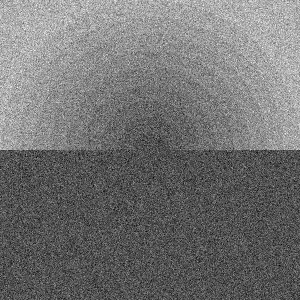
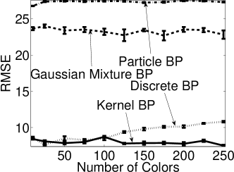
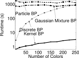
Image denoising: In our first experiment, the data consisted of grayscale images of size , resembling a sunset (Figure 1(a)). The number of colors (gray levels) in the images ranged across 10, 25, 50, 75, 100, 125, 150, 175, 200, 225 and 250, with gray levels varying evenly from 0 to 255 from the innermost ring of the sunset to the outermost. As we increased the number of colors, the grayscale transition became increasingly smooth. Our goal was to recover the original images from noisy versions, to which we had added zero mean Gaussian noise with . We compared the denoising performance and runtimes of discrete, Gaussian mixture, particle, and kernel BP.
The topology of our graphical model was a grid of hidden noise-free pixels with noisy observations made at each. The maximum degree of a node was 5 (four neighbours and an observation), and we used a template model where both the edge potentials and the likelihood functions were shared across all variables. We generated a pair of noise-free and noisy images as training data, at each color number. For kernel BP, we learned both the likelihood function and the embedding operators nonparametrically from the data. We used a Gaussian RBF kernel , with kernel bandwidth set at the median distance between training points, and residual as the stopping criterion for the feature approximation (see definition of in Section 5.1). For discrete, Gaussian mixture, and particle BP, we learned the edge potentials from data, but supplied the true likelihood of the observation given the hidden pixel (i.e., a Gaussian with standard deviation 30). This gave competing methods an important a priori advantage over kernel BP: in spite of this, kernel BP still outperformed competing approaches in speed and accuracy.
In Figure 1(c) and (d), we report the average denoising performance (RMSE: root mean square error) and runtime over 30 BP iterations, using 10 independently generated noisy test images. The RMSE of kernel BP is significantly lower than Gaussian mixture and particle BP for all numbers of colors. Although the RMSE of discrete BP is about the same as kernel BP when the number of colors is small, its performance becomes worse than kernel BP as the number of colors increases beyond 100 (despite discrete BP receiving the true observation likelihood in advance). In terms of speed, kernel BP has a considerable advantage over the alternatives: the runtime of KBP is barely affected by the number of colors. For discrete BP, the scaling is approximately square in the number of colors. For Gaussian mixture and particle BP, the runtimes are orders of magnitude longer than kernel BP, and are affected by the variability of the resampling algorithm.
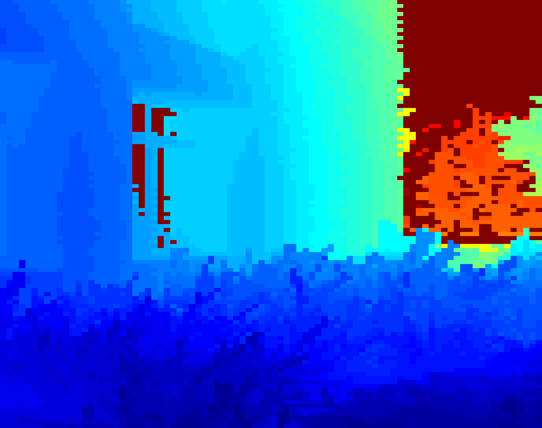
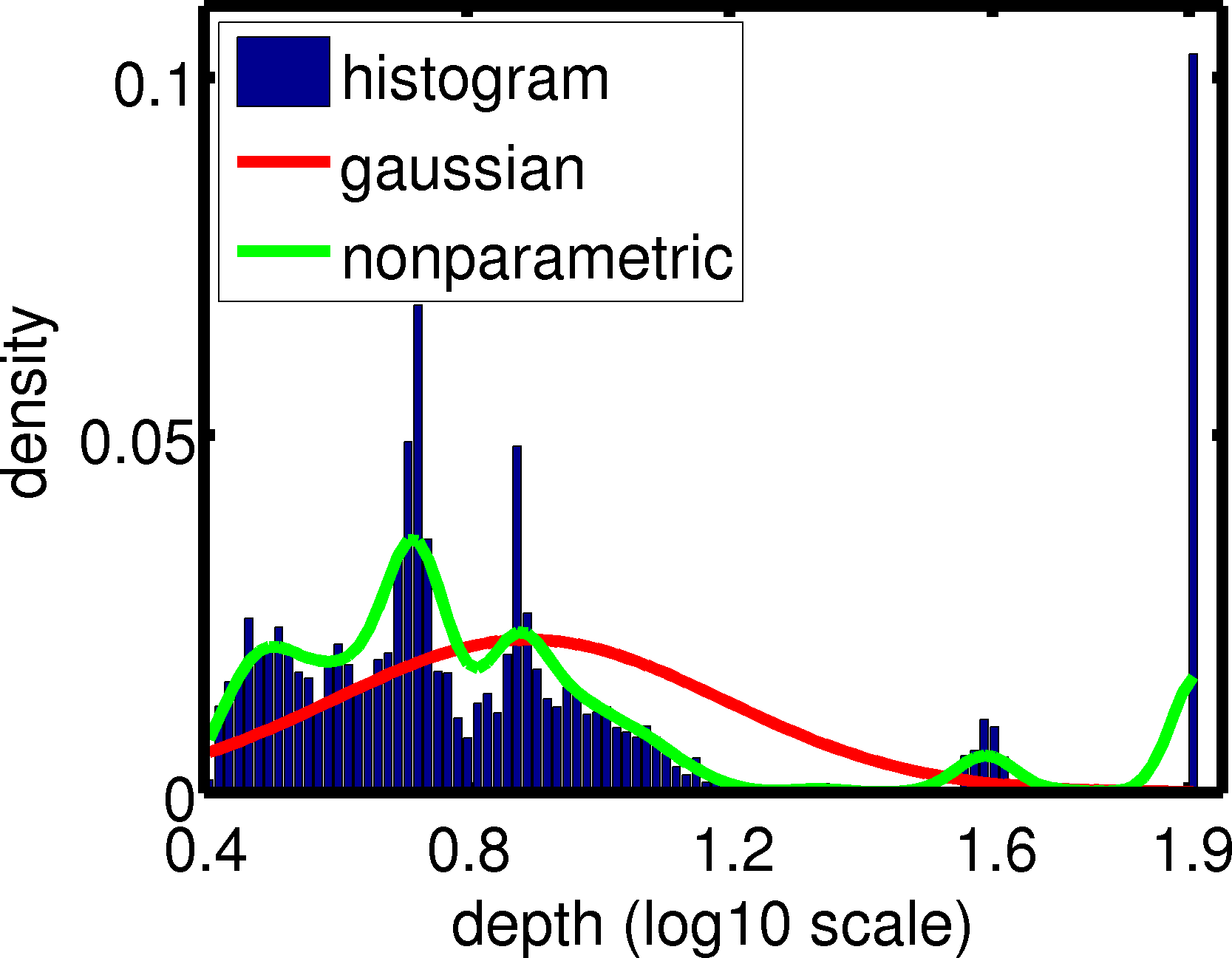
Predicting depth from 2D images: The prediction of 3D depth information from 2D image features is a difficult inference problem, as the depth may be ambiguous: similar features can occur at different depths. This creates a multimodal depth distribution given the image feature. Furthermore, the marginal distribution of the depth can itself be multimodal, which makes the Gaussian approximation a poor choice (see Figure 2(b)). To make a spatially consistent prediction of the depth map, we formulated the problem as an undirected graphical model, where a depth variable was associated with each patch of an image, and these variables were connected according to a 2D grid topology. Each hidden depth variable was linked to an image feature variable for the corresponding patch. This formulation resulted in a graphical model with continuous depth variables, and a maximum node degree of 5. Due to the way the images were taken (upright), we used a templatized model where horizontal edges in a row shared the same potential, vertical edges at the same height shared the same potential, and patches at the same row shared the same likelihood function. Both the edge potentials between adjacent depth variables and the likelihood function between image feature and depth were unknown, and were learned from data.
We used a set of 274 images taken on the Stanford campus, including both indoor and outdoor scenes (Saxena et al., 2009). Images were divided into patches of size 107 by 86, with the corresponding depth map for each patch obtained using 3D laser scanners (e.g., Figure 2(a)). Each patch was represented by a 273 dimensional feature vector, which contained both local features (such as color and texture) and relative features (features from adjacent patches). We took the logarithm of the depth map and performed learning and prediction in this space. The entire dataset contained more than 2 million data points (). We applied a Gaussian RBF kernel on the depth information, with the bandwidth parameter set to the median distance between training depths, and an approximation residual of . We used a linear kernel for the image features.

|
 |
| (a) Image and depth pair | (b) Depth distribution |
 |
 |
| (c) Depth prediction error | (d) Runtime |
 |
 |
| (a) Angle distribution | (b) Prediction accuracy |
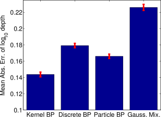
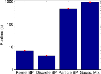
Our results were obtained by leave-one-out cross validation. For each test image, we ran discrete, Gaussian mixture, particle, and kernel BP for 10 BP iterations. The average prediction error (MAE: mean absolute error) and runtime are shown in Figures 2(c) and (d). Kernel BP produces the lowest error (MAE=0.145) by a significant margin, while having a similar runtime to discrete BP. Gaussian mixture and particle BP achieve better MAE than discrete BP, but their runtimes are two order of magnitude slower. We note that the error of kernel BP is slightly better than the results of pointwise MRF reported in Saxena et al. (2009).
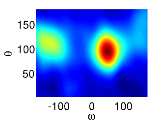
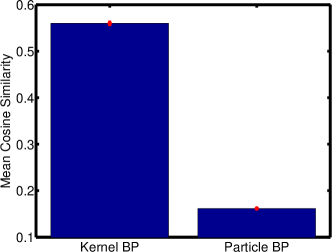
Protein structure prediction: Our final experiment investigates the protein folding problem. The folded configuration of a protein of length is roughly determined by a sequence of angle pairs , each specific to an amino acid position. The goal is to predict the sequence of angle pairs given only the amino acid sequence. The two angles have ranges and respectively, such that they correspond to points on the unit sphere . Kernels yield an immediate solution to inference on these data: Wendland (2005, Theorem 17.10) provides a sufficient condition for a function on to be positive definite, satisfied by , where is the standard inner product between Euclidean coordinates. Given the data are continuous, multimodal, and on a non-Euclidean domain (Figure 3(a)), it is not obvious how Gaussian mixture or discrete BP might be applied. We therefore focus on comparing kernel and particle BP.
We obtained a collection of proteins with length larger than 100 from PDB. We first ran PSI-BLAST to generate the sequence profile (a 20 dimensional feature for each amino acid position), and then used this profile as features for predicting the folding structure (Jones, 1999). The graphical model was a chain of connected angle pairs, where each angle pair was associated with a 20 dimensional feature. We used a linear kernel on the sequence features. For the kernel between angles, the bandwidth parameter was set at the median inner product between training points, and we used the approximation residual . For particle BP, we learned the nonparametric potentials using as the basis functions.
In Figure 3(b), we report the average prediction accuracy (Mean Cosine Similarity between the true coordinate and the predicted , i.e., ) over a 10-fold cross-validation process. In this case, kernel BP achieves a significantly better result than particle BP while running much faster (runtimes not shown due to space constraints).
8 Conclusions and Further Work
We have introduced kernel belief propagation, where the messages are functions in an RKHS. Kernel BP performs learning and inference on challenging graphical models with structured and continuous random variables, and is more accurate and much faster than earlier nonparametric BP algorithms. A possible extension to this work would be to kernelize tree-reweighted belief propagation (Wainwright et al., 2003). The convergence of kernel BP is a further challenging topic for future work (Ihler et al., 2005).
Acknowledgements: We thank Alex Ihler for the Gaussian mixture BP codes and helpful discussions. LS is supported by a Stephenie and Ray Lane Fellowship. This research was also supported by ARO MURI W911NF0710287, ARO MURI W911NF0810242, NSF Mundo IIS-0803333, NSF Nets-NBD CNS-0721591 and ONR MURI N000140710747.
Supplementary to Kernel Belief Propagation
Section 1 contains a review of Gaussian mixture BP and particle BP, as well as a detailed explanation of our strategy for learning edge potentials for these approaches from training data. Section 2 provides parameter settings and experiment details for particle BP and discrete BP, in the synthetic image denoising and depth reconstruction experiments. Section 3 contains a comparison of two different approximate feature sets: low rank approximation of the tensor features and low rank approximation of the individual features alone. Section 4 is an experiment on learning paper categories using citation networks. Sections 5 and 6 demonstrate the optimization objective of locally consistent BP updates, and provide a derivation of these updates in terms of the conditional expectation. Section 7 discusses the kernelization of Gaussian BP. Section 8 gives the error introduced by low rank approximation of the messages.
1 Gaussian Mixture and Particle BP
We describe two competing approaches for nonparametric belief propagation: Gaussian mixture BP, originally known as non-parametric BP (Sudderth et al., 2003), and particle BP (Ihler & McAllester, 2009). For these algorithms, the edge potentials , self-potentials , and evidence potentials must be provided in advance by the user. Thus, we begin by describing how the edge potentials in Section 2 of the main document may be learned from training data, but in a form applicable to these inference algorithms: we express as a mixture of Gaussians. We then describe the inference algorithms themselves.
In learning the edge potentials, we turn to Sugiyama et al. (2010), who provide a least-squares estimate of a conditional density in the form of a mixture of Gaussians,
where is a Gaussian with diagonal covariance centred at111These centres may be selected at random from the training observations. We denote the mixture kernel by to distinguish it from the RKHS kernels used earlier. . Given a training set , we obtain the coefficients
where , , is a regularization coefficient, and sets all negative entries of its argument to zero (the integral in can easily be computed in closed form). We emphasize that the Gaussian mixture representation takes a quite different form to the RKHS representation of the edge potentials. Finally, to introduce evidence, we propose to use kernel ridge regression to provide a mean value of the hidden variable given the observation , and to center a Gaussian at this value: again, the regression function is learned nonparametrically from training data.
We now describe how these edge potentials are incorporated into Gaussian mixture BP. Assuming the incoming messages are each a mixture of Gaussians, the product of such messages will contain Gaussians, which causes an exponential blow-up in representation size and computational cost. In their original work, Sudderth et al. address this issue using an approximation scheme. First, they subsample from the incoming mixture of Gaussians to draw Gaussians, at a computational cost of for each node, where is the number of iterations of the associated Gibbs sampler (see their Algorithm 1). The evidence introduced via kernel ridge regression is then incorporated, using a reweighting described by their Algorithm 2. Finally, in Algorithm 3, samples are drawn from the reweighted mixture of Gaussians, and for each of these, are drawn from the conditional distribution arising from the edge potential (which is itself a Gaussian mixture, learned via the approach of Sugiyama et al.). Gaussians are placed on each of the centres , and the process is iterated.
In our implementation, we used the more efficient multiscale KD-tree sampling method of Ihler et al. (2003). We converted the Matlab Mex implementation of Ihler (2003) to C++, and used GraphLab to execute sampling in parallel with up to 16 cores. An input parameter to the sampling procedure is , the level of accuracy. We performed a line search to set for high accuracy, but limited the execution time to be at most 1000 times slower than KBP.
Finally, we describe the inference procedure performed by Particle BP. In this case, each node is associated with a set of particles , drawn i.i.d. from a distribution . Incoming messages are expressed as weights of the particles . Unlike Gaussian mixture BP, the incoming messages all share the same set of particles, which removes the need for Parzen window smoothing. The outgoing message is computed by summing over the product of these weights and the edge and evidence potentials at the particles, yielding a set of weights over samples at node ; the procedure is then iterated (see Ihler & McAllester, 2009, eq. 8). We again implement this algorithm using edge potentials computed according to Sugiyama et al. Since an appropriate sample distribution is hard to specify in advance, a resampling procedure must be carried out at each BP iteration, to refresh the set of samples at each node and ensure the samples cover an appropriate support (this is a common requirement in particle filtering). Thus, each iteration of Particle BP requires a Metropolis-Hastings chain to be run for every node, which incurs a substantial computational cost. That said, we found that in practice, the resampling could be conducted less often without an adverse impact on performance, but resulting in major improvements in runtime, as described in Section 2 below. See (Ihler & McAllester, 2009, Section 6) for more detail.
2 Settings for Discrete and Particle BP
2.1 Depth Reconstruction from 2-D Images
2.1.1 Discrete BP
The log-depth was discretized into 30 bins, and edge parameters were selected to achieve locally consistent Loopy BP marginals using the technique described in Wainwright et al. (2003). Empirically, finer discretizations did not improve resultant accuracy, but increased runtime significantly. We used the Splash scheduling of Gonzalez et al. (2009) since it provided the lowest runtime among all tested schedulings.
2.1.2 Particle BP
The particle belief propagation implementation was particularly difficult to tune due to its excessively high runtime. Theoretically, results comparable to the Kernel BP method were attainable. However in practice, the extremely high cost of the resampling phase on large models meant that only a small number of particles could be maintained if a reasonable runtime was to be achieved on our evaluation set of 274 images.
Ultimately, we decided to find a configuration which allowed us to complete the evaluation in about 2 machine-days on an 8-core Intel Nehalem machine; allowing inference on each evaluation image to take 10 minutes of parallel computation. For each image, we ran 100 iterations of a simple linear-sweep scheduling, using 20 particles per message, and resampling every 10 iterations. Each resampling phase ran MCMC for a maximum of 10 steps per particle. We also implemented acceleration tricks where low weight particles ( after normalization) were ignored during the message passing process. Empirically this decreased runtime without affecting the quality of results.
2.2 Synthetic Image Denoising
2.2.1 Discrete BP
To simplify evaluation, we permitted a certain degree of “oracle” information, by matching the discretization levels during inference with the color levels in the ground-truth image.
We evaluated combined gradient/IPF + BP methods here to learn the edge parameters. We found that gradient/IPF performed well when there were few colors in the image, but failed to converge when the number of colors increased into the hundreds. This is partly due to the instability of BP, as well as the large number of free parameters in the edge potential.
Therefore once again, edge potentials were selected using the technique described in Wainwright et al. (2003). This performed quite well empirically, as seen in Figure 1(c) (main document).
2.2.2 Particle BP
The high runtime of the Particle Belief Propagation again made accuracy evaluation difficult. As before, we tuned the particle BP parameters to complete inference on the evaluation set of 110 images in 2 machine days, allowing about 25 minutes per evaluation image. We ran 100 iterations of 30 particles per message, resampling every 15 iterations. Each resampling phase ran MCMC for a maximum of 10 steps per particle.
3 Effects of Approximate Message Updates
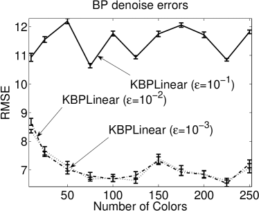
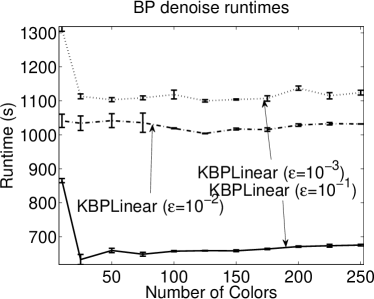
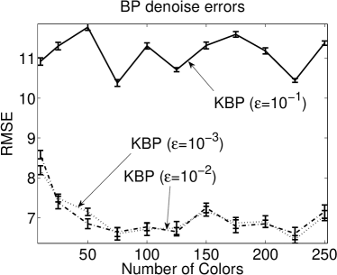
In this section, we study how different levels of feature approximation error affect the speed of kernel BP and the resulting performance. Our experimental setup was the image denoising experiment described in Section 5.1 of the main document. We note that the computational cost of our constant message update is where is inversely related to the approximation error . This is a substantial runtime improvement over naively applying a low rank kernel matrix approximation, which only results in a linear time update with computational cost . In this experiment, we varied the feature approximation error over three levels, i.e. , and compared both speed and denoising performance of the constant time update to the linear time update.
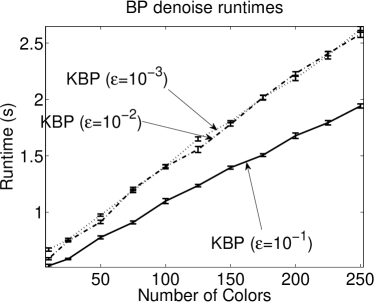
From Figures 4 (a) and (c), we can see that for each approximation level, the constant time update achieves about the same denoising performance as the linear time update, while at the same time being orders of magnitude faster (by comparing Figures 4 (b) and (d)). Despite the fact that the constant time update algorithm makes an additional approximation to the tensor product features, its denoising performance is not affected. We hypothesize that the degradation in performance is largely caused by representing the messages in terms of a small number of basis functions, while the approximation to the tensor features introduces little additional degradation.
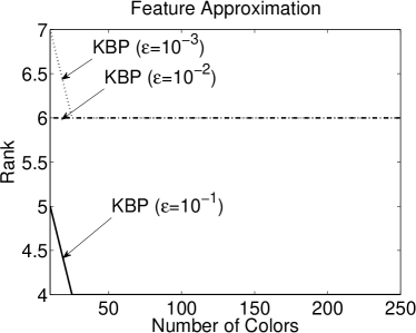
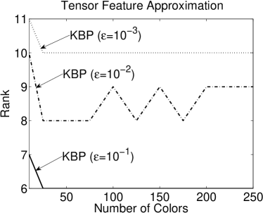
Another interesting observation from Figure 4 (d) is that the runtime of constant time kernel BP update increases as the number of colors in the image increases. This is mainly due to the increased number of test points as the color number increases; and also partially due to the increased rank needed for approximating the tensor features. In Figure 5, we plot the rank needed for kernel feature approximation and tensor feature approximation for different numbers of colors and different approximation errors . It can be seen that in general, as we use a smaller approximation error, the rank increases, leading to a slight increase in runtime.
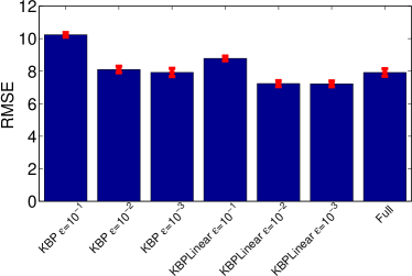
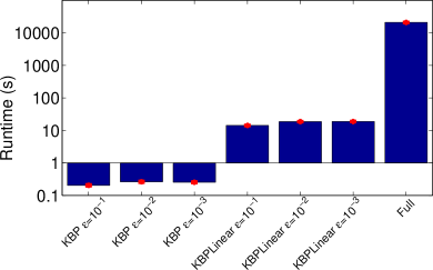
Finally, we compare with kernel belief propagation in the absence of any low rank approximation (KBP Full). Since KBP Full is computationally expensive, we reduced the denoising problem to images of size to allow KBP to finish in reasonable time. We only compared on 100 color images, again for reasons of cost. We varied the feature approximation error for the constant time and linear time approximation over three levels, , , , and compared both speed and denoising performance of KBP Full versus the constant time and linear time updates.
The comparisons are shown in Figure 6. We can see from Figure 6(a) that the denoising errors for constant time and linear time approximations decrease as we decrease the approximation error . Although the denoising error of KBP Full is slightly lower than constant time approximations, it is a slight increase over the linear time approximation at . One reason might be that the kernel approximation also serves as a means of regularization when learning the conditional embedding operator. This additional regularization may have slightly improved the generalization ability of the linear time approximation scheme. In terms of runtime (Figure 6(b)), constant time approximation is substantially faster than linear time approximation and KBP Full. In particular, it is nearly 100 times faster than the linear time algorithm, and 10000 times faster than KBP Full.
 |
 |
| (a) Error (linear time approximation) | (b) Runtime (linear time approximation) |
 |
 |
| (c) Error (constant time approximation) | (d) Runtime (constant time approximation) |
 |
 |
| (a) Rank for feature approximation | (b) Rank for tensor feature approximation |
 |
 |
| (a) Error | (b) Runtime (vertical axis is in log scale) |
4 Predicting Paper Categories
In this experiment, we predict paper categories from a combination of the paper features and their citation network. Our data were obtained by crawling 143,086 paper abstracts from the ACM digital library, and extracting the citation networks linking these papers. Each paper was labeled with a variable number of categories, ranging from 1 to 10; there were a total of 367 distinct categories in our dataset. For simplicity, we ignored directions in the citation network, and treated it as an undirected graph (i.e, we did not distinguish “citing” and “being cited”). The citation network was sparse, with more than 85% of the papers having fewer than 10 links. The maximum number of links was 450.
Paper category prediction is a multi-label problem with a large output space. The output is very sparse: the label vectors have only a small number of nonzero entries. In this case, the simple one-against-all approach of learning a single predictor for each category can become prohibitively expensive, both in training and in testing. Recently, Hsu et al. (2009) proposed to solve this problem using compressed sensing techniques: high dimensional sparse category labels are first compressed to lower dimensional real vectors using a random projection, and regressors are learned for these real vectors. In the testing stage, high dimensional category labels are decoded from the predicted real vectors of the test data using orthogonal marching pursuit (OMP).
For the purposed of the present task, however, the compressed sensing approach ignores information from the citation network: papers that share categories tend to cite each other more often. Intuitively, taking into account category information from neighboring papers in the citation network should improve the performance of category prediction. This intuition can be formalized using undirected graphical models: each paper contains a category variable , and these variables are connected according to the citation network; each category variable is also connected to a variable corresponding to the abstract of the paper. In our experiment, we used 9700 stem words for the abstracts, and was the tf-idf vector for paper . The graphical model thus contains two types of edge potential, and , where is the neighbor of according to the citation network.
It is difficult to learn this graphical model and perform inference on it, since the category variables have high cardinality, making the marginalization step in BP prohibitively expensive. Inspired by the compressed sensing approach for multilabel prediction, we first employed random projection kernels, and then used our kernel BP algorithm. Let be a random matrix containing i.i.d. Gaussian random variables of zero mean and variance . We defined the random projection kernel for the category labels to be , and used a linear kernel for the abstract variables. We ran kernel BP for 5 iterations, since further iterations did not improve the performance. MAP assignment based on the belief was performed by finding a unit vector that maximized the belief. The sparse category labels were decoded from using OMP.
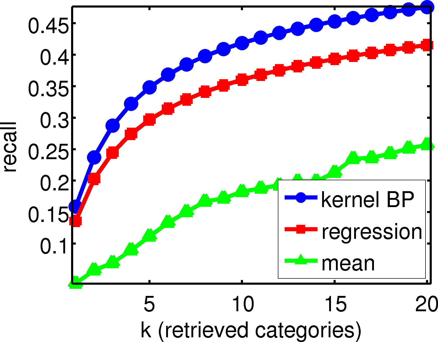
To measure experimental performance, we performed 10 random splits of the papers, where in each split we used 1/3 of the papers for training and the remaining 2/3 for testing. The random splits were controlled in such a way that high degree nodes (with degree ) in the citation networks always appeared in the training set. Such splitting reflects the data properties expected in real-world scenarios: important papers (high degree nodes which indicate either influential papers or survey papers) are usually labeled, whereas the majority of papers may not have a label; the automatic labeling is mainly needed for these less prominent papers. We used recall@ in evaluating the performance of our method on the test data. We compared against the regression technique of Hsu et al. for multilabel prediction, and a baseline prediction using the top most frequent categories. For both our method and the method of Hsu et al., we used a random projection matrix with .
Results are shown in Figure 7. Kernel BP performs better than multilabel prediction via compressed sensing (i.e., the independent regression approach, which ignores graphical model structure) over a range of values. In particular, for the top 10 and 20 predicted categories, kernel BP achieves recall scores of 0.419 and 0.476, respectively, as opposed to 0.362 and 0.417 for independent regression.
5 Local Marginal Consistency Condition When Learning With BP
In this section, we show that fixed points of BP satisfy particular marginal consistency conditions (29) and (30) below. As we will see, these arise from the fact that we are using a Bethe free energy approximation in fitting our model, and the form of the fixed point equations that define the minimum of the Bethe free energy. The material in this section draws from a number of references (for instance Yedidia et al., 2001, 2005; Wainwright & Jordan, 2008; Koller & Friedman, 2009), but is presented in a form specific to our case, since we are neither in a discrete domain nor using exponential families.
The parameters of a pairwise Markov random field (MRF) can be learned by maximizing the log-likelihood of the model with respect to true underlying distribution . Denote the model by
where is the partition function that normalizes the distribution. The model parameters can be estimated by maximizing
| (16) |
Define and . Setting the derivatives of with respect to to zero, we have
| (17) | ||||
| (18) |
For a general pairwise MRF on a loopy graph, computing the log-partition function, , is intractable. Following e.g. Yedidia et al. (2001, 2005) and Koller & Friedman (2009, Ch. 11), may be approximated as a minimum of the Bethe free energy with respect to a new set of parameters ,
| (19) |
subject to normalization and marginalization constraints, , . Let (we note that Bethe free energy is not convex, and hence there can be multiple local minima. Our reasoning does not require constructing a specific local minimum, and therefore we simply write ). The zero gradient conditions on the partial derivatives of are then approximated as
| (20) | ||||
| (21) |
Since is a linear function of for every fixed , Danskin’s theorem (Bertsekas, 1999, p. 717) gives us a way to compute the partial derivatives of . These are
| (22) | ||||
| (23) |
where . Therefore, according to (20) and (21), learning a pairwise MRF using the Bethe energy variational approximation to the log partition function results in the following matching conditions,
| (24) | ||||
| (25) |
We now introduce the notion of belief propagation as a means of finding the minima of the Bethe free energy. This will in turn lead to local marginal consistency conditions for learning with BP. Yedidia et al. (2001) showed that the fixed point of (and therefore the global minimum ) must satisfy the relations
| (26) | ||||
| (27) |
where denotes a normalization constant and are the fixed point messages,
| (28) |
Thus,
| (29) | ||||
| (30) |
Combining these relations and assuming that and are strictly positive, we can also obtain the consistent relation for the local conditionals,
| (31) |
6 BP Inference Using Learned Potentials
The inference problem in pairwise MRFs is to compute the marginals or the log partition function for the model with learned potentials. Belief propagation is an iterative algorithm for performing approximate inference in MRFs. BP can also be viewed as an iterative algorithm for minimizing the Bethe free energy approximation to the log partition function. The results of this algorithm are a set of beliefs which can be used for obtaining the MAP assignment of the corresponding variables.
The BP message update (with the learned potentials) is
| (32) |
and at any iteration, the beliefs can be computed using the current messages,
| (33) | ||||
| (34) |
To see how the message update equation can be expressed using the true local conditional , we divide both size of (32) by the fixed point message during BP learning stage, and introduce . The message update equation in (32) can then be re-written as
| (35) |
The belief at any iteration becomes
| (36) |
We reparameterize the message as
| (37) |
Since the potentials are learned via BP, we can use the relation in (31) to obtain
| (38) |
Similarly, we obtain from (30) that
| (39) |
Messages from Evidence Node
Given evidence at node , the outgoing message from to is . Using similar reasoning to the case of an internal node, we have
| (40) | ||||
| (41) | ||||
| (42) | ||||
| (43) |
where is constant given a fixed value . Reparametrizing the message , the outgoing message from the evidence node is simply the true likelihood function evaluated at .
7 A Note on Kernelization of Gaussian BP
In this section, we consider the problem of defining a joint Gaussian graphical model in the feature space induced by a kernel. We follow Bickson (2008) in our presentation of the original Gaussian BP setting. We will show that assuming a Gaussian in an infinite feature space leads to challenges in interpretation and estimation of the model.
Consider a pairwise MRF,
| (44) |
In the case of the Gaussian, the probability density function takes the form
where is the precision matrix, and
Putting this in the form (44), the node and edge potentials are written
| (45) |
and
| (46) |
We now consider how these operations would appear in Hilbert space. In this case, we would have
and
We call the and precision operators, by analogy with the finite dimensional case. At this point, we already encounter a potential difficulty in kernelizing Gaussian BP: how do we learn the operators , and from data? We could in principle define a covariance operator with th block the pairwise covariance operator , but would then be the th block of , which is difficult to compute. As we shall see below, however, these operators appear in the BP message updates.
Next, we describe a message passing procedure for the Gaussian potentials in (45) and (46). The message from to is written
We first consider term (a) in the above. We will assume, with justification to follow, that takes the form
where the terms and are defined by recursions specified below (we retain linear algebraic notation for simplicity). It follows that is proportional to a Gaussian,
where we define the intermediate operators
and
To compute the message , we integrate
| (47) | |||||
Completing the square, we get the parameters of the message in the standard form,
| (48) | ||||
| (49) |
There are two main difficulties in implementing the above procedure in feature space. First, it is not clear how to learn the precision operators from the data. Second, we need to invert these precision operators. Thus, it remains a challenging open question to define Gaussian BP in feature space. The feature space Gaussian BP updates may be contrasted with the kernel BP updates we propose in the main text. The latter have regularized closed form empirical estimates, and they are very different from the Gaussian BP form in (47) and parameter updates in (48) and (49).
8 Message Error Incurred by the Additional Feature Approximation
We bound the difference between the estimated conditional embedding operator and its counterpart after further feature approximation. Assume , and define the tensor feature . Denote by and the respective approximations of and . Furthermore, let the approximation error after the incomplete QR decomposition be . It follows that
| (50) | ||||
| (51) | ||||
| (52) | ||||
| (53) |
For the first term,
| (54) | ||||
| (55) | ||||
| (56) | ||||
| (57) | ||||
| (58) | ||||
| (59) |
Similarly, for the second term,
| (60) |
Combining the results, we obtain
| (61) |
References
- Aronszajn (1950) Aronszajn, N. (1950). Theory of reproducing kernels. Trans. Amer. Math. Soc., 68, 337–404.
- Bach & Jordan (2002) Bach, F. R., & Jordan, M. I. (2002). Kernel independent component analysis. J. Mach. Learn. Res., 3, 1–48.
- Bickson et al. (2011) Bickson, D., Baron, D., Ihler, A., Avissar, H., & Dolev, D. (2011). Fault identification via non-parametric belief propagation. IEEE Transactions on Signal Processing. ISSN 1053-587X.
- Fukumizu et al. (2004) Fukumizu, K., Bach, F. R., & Jordan, M. I. (2004). Dimensionality reduction for supervised learning with reproducing kernel Hilbert spaces. J. Mach. Learn. Res., 5, 73–99.
- Fukumizu et al. (2009) Fukumizu, K., Sriperumbudur, B., Gretton, A., & Schoelkopf, B. (2009). Characteristic kernels on groups and semigroups. In Advances in Neural Information Processing Systems 21, 473–480. Red Hook, NY: Curran Associates Inc.
- Ihler & McAllester (2009) Ihler, A., & McAllester, D. (2009). Particle belief propagation. In AISTATS.
- Ihler et al. (2005) Ihler, A. T., Fisher III, J. W., & Willsky, A. S. (2005). Loopy belief propagation: Convergence and effects of message errors. J. Mach. Learn. Res., 6, 905–936.
- Ihler et al. (2003) Ihler, E. T., Sudderth, E. B., Freeman, W. T., & Willsky, A. S. (2003). Efficient multiscale sampling from products of gaussian mixtures. In In NIPS 17.
- Jones (1999) Jones, D. T. (1999). Protein secondary structure prediction based on position-specific scoring matrices. J. Mol. Biol., 292, 195–202.
- Koller & Friedman (2009) Koller, D., & Friedman, N. (2009). Probabilistic Graphical Models: Principles and Techniques. MIT Press.
- Low et al. (2010) Low, Y., Gonzalez, J., Kyrola, A., Bickson, D., Guestrin, C., & Hellerstein, J. M. (2010). GraphLab: A new parallel framework for machine learning. In Conference on Uncertainty in Artificial Intelligence.
- McEliece et al. (1998) McEliece, R., MacKay, D., & Cheng, J. (1998). Turbo decoding as an instance of Pearl’s ‚Äúbelief propagation‚Äù algorithm. J-SAC.
- Murphy et al. (1999) Murphy, K. P., Weiss, Y., & Jordan, M. I. (1999). Loopy belief propagation for approximate inference: An empirical study. In UAI, 467–475.
- Pearl (1988) Pearl, J. (1988). Probabilistic Reasoning in Intelligent Systems: Networks of Plausible Inference. Morgan Kaufman.
- Saxena et al. (2009) Saxena, A., Sun, M., & Ng, A. Y. (2009). Make3d: Learning 3d scene structure from a single still image. IEEE Trans. Pattern Anal. Mach. Intell., 31(5), 824–840. ISSN 0162-8828. doi:http://dx.doi.org/10.1109/TPAMI.2008.132.
- Schölkopf & Smola (2002) Schölkopf, B., & Smola, A. (2002). Learning with Kernels. Cambridge, MA: MIT Press.
- Schölkopf et al. (2004) Schölkopf, B., Tsuda, K., & Vert, J.-P. (2004). Kernel Methods in Computational Biology. Cambridge, MA: MIT Press.
- Shawe-Taylor & Cristianini (2004) Shawe-Taylor, J., & Cristianini, N. (2004). Kernel Methods for Pattern Analysis. Cambridge, UK: Cambridge University Press.
- Song et al. (2010) Song, L., Gretton, A., & Guestrin, C. (2010). Nonparametric tree graphical models. In 13th Workshop on Artificial Intelligence and Statistics, vol. 9 of JMLR workshop and conference proceedings, 765–772.
- Song et al. (2009) Song, L., Huang, J., Smola, A., & Fukumizu, K. (2009). Hilbert space embeddings of conditional distributions. In Proc. Intl. Conf. Machine Learning.
- Steinwart (2001) Steinwart, I. (2001). On the influence of the kernel on the consistency of support vector machines. J. Mach. Learn. Res., 2, 67–93.
- Sudderth et al. (2003) Sudderth, E., Ihler, A., Freeman, W., & Willsky, A. (2003). Nonparametric belief propagation. In CVPR.
- Sugiyama et al. (2010) Sugiyama, M., Takeuchi, I., Suzuki, T., Kanamori, T., Hachiya, H., & Okanohara, D. (2010). Conditional density estimation via least-squares density ratio estimation. 781–788.
- Wainwright et al. (2003) Wainwright, M., Jaakkola, T., & Willsky, A. (2003). Tree-reweighted belief propagation and approximate ML estimation by pseudo-moment matching. In 9th Workshop on Artificial Intelligence and Statistics.
- Wainwright & Jordan (2008) Wainwright, M. J., & Jordan, M. I. (2008). Graphical models, exponential families, and variational inference. Foundations and Trends in Machine Learning, 1(1 – 2), 1 – 305.
- Weiss & Freeman (2001) Weiss, Y., & Freeman, W. T. (2001). Correctness of belief propagation in Gaussian graphical models of arbitrary topology. Neural Computation, 13, 2173–2200.
- Wendland (2005) Wendland, H. (2005). Scattered Data Approximation. Cambridge, UK: Cambridge University Press.
- Yanover & Weiss (2002) Yanover, C., & Weiss, Y. (2002). Approximate inference and protein-folding. In NIPS, 1457–1464. MIT Press.
- Yedidia et al. (2001) Yedidia, J. S., Freeman, W. T., & Weiss, Y. (2001). Generalized belief propagation. In T. K. Leen, T. G. Dietterich, & V. Tresp, eds., Advances in Neural Information Processing Systems 13, 689–695. MIT Press.
- Bertsekas (1999) Bertsekas, D. P. (1999). Nonlinear Programming. Belmont, MA: Athena Scientific, second edn.
- Bickson (2008) Bickson, D. (2008). Gaussian Belief Propagation: Theory and Application. Ph.D. thesis, The Hebrew University of Jerusalem.
- Gonzalez et al. (2009) Gonzalez, J., Low, Y., & Guestrin, C. (2009). Residual splash for optimally parallelizing belief propagation. In In Artificial Intelligence and Statistics (AISTATS). Clearwater Beach, Florida.
- Hsu et al. (2009) Hsu, D., Kakade, S. M., Langford, J., & Zhang, T. (2009). Multi-label prediction via compressed sensing. In Advances in Neural Information Processing Systems 21.
- Ihler (2003) Ihler, A. (2003). KDE Matlab ToolBox. http://www.ics.uci.edu/ ihler/code/.
- Ihler & McAllester (2009) Ihler, A., & McAllester, D. (2009). Particle belief propagation. In AISTATS, 256–263.
- Ihler et al. (2003) Ihler, E. T., Sudderth, E. B., Freeman, W. T., & Willsky, A. S. (2003). Efficient multiscale sampling from products of gaussian mixtures. In Advances in Neural Information Processing Systems 17.
- Koller & Friedman (2009) Koller, D., & Friedman, N. (2009). Probabilistic Graphical Models: Principles and Techniques. MIT Press.
- Sudderth et al. (2003) Sudderth, E., Ihler, A., Freeman, W., & Willsky, A. (2003). Nonparametric belief propagation. In CVPR.
- Sugiyama et al. (2010) Sugiyama, M., Takeuchi, I., Suzuki, T., Kanamori, T., Hachiya, H., & Okanohara, D. (2010). Conditional density estimation via least-squares density ratio estimation. In AISTATS, 781–788.
- Wainwright et al. (2003) Wainwright, M., Jaakkola, T., & Willsky, A. (2003). Tree-reweighted belief propagation and approximate ML estimation by pseudo-moment matching. In 9th Workshop on Artificial Intelligence and Statistics.
- Wainwright & Jordan (2008) Wainwright, M. J., & Jordan, M. I. (2008). Graphical models, exponential families, and variational inference. Foundations and Trends in Machine Learning, 1(1 – 2), 1 – 305.
- Yedidia et al. (2005) Yedidia, J., Freeman, W., & Weiss, Y. (2005). Constructing free-energy approximations and generalized belief propagation algorithms. IEEE Transactions on Information Theory, 51(7), 2282 – 2312.
- Yedidia et al. (2001) Yedidia, J. S., Freeman, W. T., & Weiss, Y. (2001). Generalized belief propagation. In T. K. Leen, T. G. Dietterich, & V. Tresp, eds., Advances in Neural Information Processing Systems 13, 689–695. MIT Press.