Memory Effects In Nonequilibrium Quantum Impurity Models

Abstract

Memory effects play a key role in the dynamics of strongly correlated systems driven out of equilibrium. In the present study, we explore the nature of memory in the nonequilibrium Anderson impurity model. The Nakajima–Zwanzig–Mori formalism is used to derive an exact generalized quantum master equation for the reduced density matrix of the interacting quantum dot, which includes a non-Markovian memory kernel. A real-time path integral formulation is developed, in which all diagrams are stochastically sampled in order to numerically evaluate the memory kernel. We explore the effects of temperature down to the Kondo regime, as well as the role of source–drain bias voltage and band width on the memory. Typically, the memory decays on timescales significantly shorter than the dynamics of the reduced density matrix itself, yet under certain conditions it develops a smaller long tail. In addition we address the conditions required for the existence, uniqueness and stability of a steady-state.

Interest in the problem of intrinsically nonequilibrium open quantum systems—in which one considers a small, strongly interacting and highly correlated region coupled to several large, noninteracting baths—has been surging in both experiment and theory. The aim of theory in this regard is to provide a solid framework for understanding phenomena ranging from the nonequilibrium Kondo effect in quantum dots to conductance through single molecules nitzan_electron_2003 . While much progress has been made recently, based on brute-force approaches such as time-dependent numerical renormalization group techniques anders_real-time_2005 ; white_density_1992 ; schmitteckert_nonequilibrium_2004 and iterative weiss_iterative_2008 ; segal_numerically_2010 or stochastic muehlbacher_real-time_2008 ; werner_diagrammatic_2009 ; schiro_real-time_2009 diagrammatic approaches to real-time path integral formulations, the problem has never been fully solved in a satisfactory manner. In fact, it is becoming clearer that major gaps exist in our understanding of the dynamics, the crossover regimes, the dependence on initial conditions and the behavior at steady state.

The kind of open systems discussed above are often addressed by impurity models, which explicitly account for the two types of regions within the problem by partitioning the Hamiltonian into system and bath subspaces: $H=H_{S}+H_{B}+V$, where $H_{S}$ represents a low-dimensional but interacting “system” subspace, $H_{B}$ represents a set of non-interacting lead or bath subspaces, and $V$ is a system–bath coupling term. The dynamics generated by such Hamiltonians can feature transients on timescales that are much longer than the typical inverse energy scale nordlander_how_1999 , where numerically exact approaches become intractable due to the exponential growth of the active space or the equivalent complications resulting from the dynamical sign problem. In many important situations, however, the non-interacting baths can be traced out, leading to a reduced description of the dynamics of the interacting system at the cost of introducing non-locality in the time propagation feynman_theory_1963 . In path integral approaches the effects of the leads are accounted for by a time non-local influence functional muehlbacher_real-time_2008 ; weiss_iterative_2008 .

Perhaps a more appealing approach, which has been used to derive very successful perturbative schemes for fermionic systems leijnse_kinetic_2008 ; li_coherent_2010 but is notoriously difficult to carry out exactly, is based on the generalized quantum master equation (GQME). In this formalism, a so-called memory kernel replaces the influence functional. The complexity of solving the many-body quantum Liouville equation is then reduced to the evaluation of this memory kernel, which fully determines the dynamics of the system. Furthermore, the memory kernel contains all the information needed to resolve questions concerning the existence and uniqueness of a steady-state dhar_nonequilibrium_2006 ; khosravi_bound_2009 , as well as the values of system observables at steady state. While the dynamical timescale of the system typically exceeds the characteristic inverse energy scale, the memory kernel is expected to decay on relatively short timescales for a large and interesting class of physical situations (essentially whenever the bandwidth of the baths is much larger than other energy scales in the problem). Thus, brute-force approaches limited to short times are well suited to its calculation. Once the memory function is known, the formalism is exact and tractable at all times.

In this Letter, we explore the nature of memory in nonequilibrium impurity models, and focus on the Anderson problem anderson_localized_1961 , covering the effects of temperature down to the Kondo regime, the role of source–drain bias voltages and band width. This is accomplished by adopting the Nakajima–Zwanzig–Mori nakajima_quantum_1958 ; zwanzig_ensemble_1960 ; mori_transport_1965 formalism to derive an exact GQME for the reduced density matrix $\sigma\left(t\right)=P\rho\left(t\right)$ of the interacting system, which includes a non-Markovian memory kernel. The conjecture that the memory decays on timescales significantly shorter than the dynamics of $\sigma\left(t\right)$ is confirmed, yet it is found that it develops a smaller long tail when the Hubbard term is switched on. The approach provides means to simulate the dynamics of the strongly correlated subsystem on timescales beyond the limits of the path integral method itself and reveals the conditions required for the existence, uniqueness and stability of a steady-state under a finite source-drain bias.

Figure 1: Distinct nonzero memory kernel elements for an initially unoccupied dot and several values of the interaction energy $U$. The remaining parameters are $\frac{\mu_{L}}{\Gamma}=-\frac{\mu_{R}}{\Gamma}=\frac{1}{2}$, $\frac{\varepsilon_{c}}{\Gamma}=20$, and $\beta\Gamma=1$.

The exact equation of motion of the complete density matrix, $i\hbar\frac{\mathrm{d}}{\mathrm{d}t}\rho=\left[H,\rho\right]$, is governed by the Liouvillian $\mathcal{L}=\left[H,\,...\right]$. If the coupling term $V$ were to be turned off, the dynamics of the two subspaces would be given by similar equations with the Liouvillian replaced by the system and bath Liouvillians, $\mathcal{L}_{S}=\left[H_{S},\,...\right]$ and $\mathcal{L}_{B}=\left[H_{B},\,...\right]$, respectively. We also define a coupling Liouvillian $\mathcal{L}_{V}=\left[V,\,...\right]$. The equation of motion for the reduced density operator $\rho_{B}\sigma=P\rho$ (using the projection operator onto the system subspace $P=\rho_{B}\mathrm{Tr}_{B}\left\{...\right\}$) is then given by:

$$i\hbar\frac{\mathrm{d}}{\mathrm{d}t}\sigma\left(t\right)=\mathcal{L}_{S}\sigma\left(t\right)+\vartheta\left(t\right)-\frac{i}{\hbar}\int_{0}^{t}\mathrm{d}\tau\,\kappa\left(\tau\right)\sigma\left(t-\tau\right),$$ (1)

where $\vartheta\left(t\right)=\mathrm{Tr}_{B}\left\{\mathcal{L}_{V}e^{-\frac{i}{\hbar}Q\mathcal{L}t}Q\rho_{0}\right\}$ contains the initial correlations, $\kappa\left(t\right)=\mathrm{Tr}_{B}\left\{\mathcal{L}_{V}e^{-iQ\mathcal{L}\tau}Q\mathcal{L}\rho_{B}\right\}$ is the memory kernel in superoperator form, and $Q=1-P$. The initial condition are contained within the initial density matrix $\rho_{0}$, which also determines the initial bath part of the density matrix $\rho_{B}=Q\rho_{0}$.

The above equation for $\sigma\left(t\right)$ is exact, yet requires as input the two superoperator functions $\kappa\left(t\right)$ and $\vartheta\left(t\right)$, both of which have been defined in terms of projected propagation. Evaluating such projected dynamics is cumbersome, and can be reduced to solving a superoperator Volterra equation of the second type involving a quantity $\Phi\left(t\right)$ which is free of projected propagation zwanzig_nonequilibrium_2001 ; zhang_nonequilibrium_2006 . For the memory kernel one finds:

$$\kappa\left(\tau\right) = i\hbar\dot{\Phi}\left(\tau\right)-\Phi\left(\tau\right)\mathcal{L}_{S}$$ (2)

$$\,+\frac{i}{\hbar}\int_{0}^{\tau}\mathrm{d}\tau\Phi\left(t-\tau\right)\kappa\left(\tau\right),$$

$$\Phi\left(t\right) = \mathrm{Tr}_{B}\left\{\mathcal{L}_{V}e^{-\frac{i}{\hbar}\mathcal{L}t}\rho_{B}\right\}.$$ (3)

A similar procedure exists for the initial correlation term $\vartheta$; however, here we consider only the initially factorized case $\rho_{0}=\rho_{B}\otimes\sigma\left(0\right)$, for which $\vartheta=0$. As discussed below, the matrix elements of the superoperator $\Phi$ are identical to quantities to which RT-PIMC has already been applied muehlbacher_real-time_2008 ; werner_diagrammatic_2009 .

In the Anderson impurity model $H_{S}=\sum_{i=\uparrow\downarrow}\varepsilon_{i}d_{i}^{\dagger}d_{i}+Ud_{\uparrow}^{\dagger}d_{\uparrow}d_{\downarrow}^{\dagger}d_{\downarrow}$, $H_{B}=\sum_{k,i=\uparrow\downarrow}\varepsilon_{ik}a_{ik}^{\dagger}a_{ik}$ and $V=\sum_{ki=\uparrow\downarrow}t_{ik}d_{i}a_{ik}^{\dagger}+t_{ik}^{*}a_{ik}d_{i}^{\dagger}$. Thus, the system subspace is four-dimensional, being spanned by the states $0\equiv\left|00\right\rangle\equiv\left|0\right\rangle,\,1\equiv\left|01\right\rangle=d_{2}^{\dagger}\left|0\right\rangle,\,2\equiv\left|10\right\rangle=d_{1}^{\dagger}\left|0\right\rangle$ and $3\equiv\left|11\right\rangle=d_{1}^{\dagger}d_{2}^{\dagger}\left|0\right\rangle$. With this notation, we can perform a calculation to derive an expression for the system Liouvillian

$$\left[\mathcal{L}_{s}\right]_{ij,qq^{\prime}} = \delta_{iq}\delta_{jq^{\prime}}\left\{\varepsilon_{1}\left(\delta_{q2}+\delta_{q3}-\delta_{j2}-\delta_{j3}\right)\right.$$ (4)

$$\,+\varepsilon_{2}\left(\delta_{q1}+\delta_{q3}-\delta_{j1}-\delta_{j3}\right)$$

$$\,\left.+U\left(\delta_{q3}-\delta_{j3}\right)\right\},$$

and for $\Phi$, which takes the more complicated form

$$\Phi_{ij,qq^{\prime}} = -\delta_{i2}\delta_{j1}\left(\psi_{qq^{\prime}}^{\left(1\right)}-\psi_{qq^{\prime}}^{\left(2\right)*}\right)-\delta_{i1}\delta_{j2}\left(\psi_{qq^{\prime}}^{\left(2\right)}-\psi_{qq^{\prime}}^{\left(1\right)*}\right)$$ (5)

$$+ \delta_{ij0}\left(\varphi_{qq^{\prime}}^{\left(1\right)}+\varphi_{qq^{\prime}}^{\left(3\right)}\right)+\delta_{ij1}\left(\varphi_{qq^{\prime}}^{\left(2\right)}-\varphi_{qq^{\prime}}^{\left(3\right)}\right)$$

$$+ \delta_{ij2}\left(-\varphi_{qq^{\prime}}^{\left(1\right)}+\varphi_{qq^{\prime}}^{\left(4\right)}\right)+\delta_{ij3}\left(-\varphi_{qq^{\prime}}^{\left(2\right)}-\varphi_{qq^{\prime}}^{\left(4\right)}\right),$$

$$\varphi_{qq^{\prime}}^{\left(m\right)} = 2i\Im\sum_{k}\mathrm{Tr}_{B}\left\{\rho_{B}\left\langle q^{\prime}\right|A_{k}^{\left(m\right)}\left|q\right\rangle\right\},$$ (6)

$$\psi_{qq^{\prime}}^{\left(m\right)} = -2\sum_{k}\mathrm{Tr}_{B}\left\{\rho_{B}\left\langle q^{\prime}\right|B_{k}^{\left(m\right)}\left|q\right\rangle\right\},$$ (7)

where $A_{k}^{\left(1\right)}=t_{1k}d_{1}d_{2}d_{2}^{\dagger}a_{1k}^{\dagger}$, $A_{k}^{\left(2\right)}=t_{1k}d_{1}d_{2}^{\dagger}d_{2}a_{1k}^{\dagger}$, $A_{k}^{\left(3\right)}=t_{2k}d_{1}d_{1}^{\dagger}d_{2}a_{2k}^{\dagger}$, $A_{k}^{\left(4\right)}=t_{2k}d_{1}^{\dagger}d_{1}d_{2}a_{2k}^{\dagger}$, $B_{k}^{\left(1\right)}=t_{1k}d_{2}a_{1k}^{\dagger}$ and $B_{k}^{\left(2\right)}=t_{2k}d_{1}a_{2k}^{\dagger}$. All the quantities in (5)–(7) are implicitly time-dependent and can be evaluated directly with RT-PIMC Cohen-un .

Figure 2: Total population derivative from direct RT-PIMC data compared with the results of the memory-kernel formalism (left panels) and predicted dot populations (right panels) for an initially unoccupied dot for several values of the interaction energy $U$. Remaining parameters are the same as in Fig. 1. The cutoff time is $\frac{1.5}{\Gamma}$, shown on the right panels as a vertical dotted line.

One can draw a few analytical conclusions directly from the block structure of $\Phi$. First, while both the $A_{k}^{\left(m\right)}$ and $B_{k}^{\left(m\right)}$ operators introduced above conserve the total particle number, only the $A_{k}^{\left(m\right)}$ conserve the particle number for each spin. Therefore, the $\psi_{qq^{\prime}}^{\left(m\right)}$ are nonzero only if $q,q^{\prime}=1,2$ or $2,1$ (since states $1$ and $2$ are the only dot states which have the same total occupation, but differ in per-spin occupation), while the $\varphi_{qq^{\prime}}^{\left(m\right)}$ can be nonzero only when $q=q^{\prime}$. From (5) we can then immediately see that the diagonal density matrix elements are coupled only to each other, with the two singly occupied off-diagonal elements $\left|1\right\rangle\left\langle 2\right|$ and $\left|2\right\rangle\left\langle 1\right|$ forming a second closed block. If our interest is limited to the state populations only the $16$ (instead of $64$) functions $\varphi_{qq}^{\left(m\right)}$ need be evaluated within RT-PIMC.

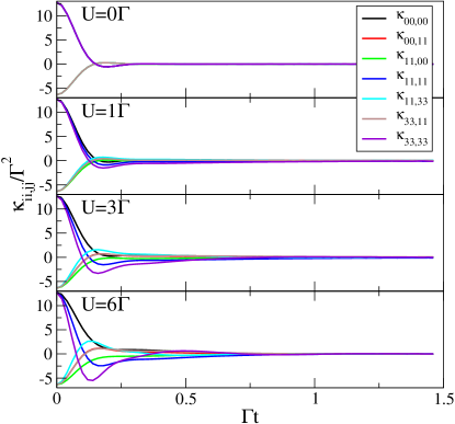
In Fig. 1, we plot the nonzero elements of the memory kernel for different values of $U$. Due to the block structure and the symmetric choice of parameters, only seven distinct nonzero elements exist (two for $U=0$). To make the parametrization definite within the simulations, we assume lead coupling densities of the form $\Gamma_{i}\left(E\right)\equiv 2\pi\sum_{k}\left|t_{k}\right|^{2}\delta\left(E-\varepsilon_{ik}\right)=\frac{\Gamma/2}{\left(1+e^{\nu\left(E-\varepsilon_{c}\right)}\right)\left(1+e^{-\nu\left(E+\varepsilon_{c}\right)}\right)}$, where $\varepsilon_{c}$ is the band cutoff energy and $\nu$ is the inverse of the cutoff width. $\Gamma$ is the maximum value attainable by $\Gamma\left(E\right)=\sum_{i}\Gamma_{i}\left(E\right)$, as well as its wide band limit, and will be the unit of energy throughout the following text. We also concentrate on $\varepsilon_{i}=-\frac{U}{2}$, known as the symmetric case of the Anderson model, yet the formalism is general and this is certainly not a requirement The temperature $\beta$ and the chemical potentials $\mu_{L}$ and $\mu_{R}$ enter the calculation through $\rho_{B}$ at time zero for which we assume the proper grand canonical distribution.

In the noninteracting case (top panel of Fig. 1), a rapid decay to zero is observed. Despite the relatively broad and soft-edged band chosen here, the decay occurs over a timescale smaller than the inverse coupling but comparable to it. We can learn from this that any approximation based on short memory should be expected to fail unless it can allow for memories of at least this length, meaning for instance that Markovian approaches to the problem cannot be expected to succeed in general. As $U$ is increased, it becomes clear that the interaction—despite breaking most of the symmetries between the various elements—does not significantly affect memory decay on the first timescale. However, even at very small interaction energies, a second, longer timescale develops: at this timescale, a small part of each memory kernel element decays more slowly.

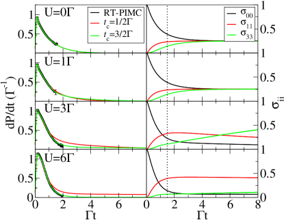
The formalism becomes extremely interesting if having the memory as an input only up to some finite cutoff time $t_{c}$—at which the system’s dynamics have not yet died out—allows accurate predictions at far longer times. This will occur if the memory function has essentially gone to zero by this time, such that it can be safely truncated. In the left panels of Fig. 2 we plot the time derivative of the total population ($dP/dt$) and show that for certain noninteracting parameters this does indeed happen: once $\Gamma t_{c}\gtrsim\frac{1}{3}$ dynamics at times over an order of magnitude greater than those of the memory kernel are reliably reproduced, and the exact steady-state result for all diagonal elements of $\sigma$ is obtained to within the numerical errors and shown on the top right panel of Fig. 2. However, as might be expected from the analysis of Fig. 1, in the strongly correlated cases a short cutoff time results in incorrect populations when propagated for much longer times than $t_{c}$, since truncating the memory at that point has not yet become physically reasonable. For the cases of $U=\Gamma$ and $U=6\Gamma$ the qualitative physics is captured correctly within $t_{c}=3/2\Gamma$ in that depopulation of the zero-electron level is accelerated at short times; for $U=6\Gamma$ one also observes that at longer times the one-electron levels draw most of the population while the more energetic zero- and two-electron levels are suppressed. However, for $U=3\Gamma$, the behavior predicted by the truncated memory function is clearly wrong, consistent with the existence of long time tails in the memory.

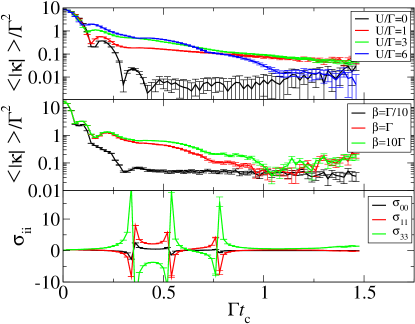
The top two panels of Fig. 3 explore the decay of the memory kernel elements more clearly by plotting the average absolute value of the memory kernel elements on a logarithmic scale, for various values of $U$, $\varepsilon_{c}$ and $\beta$. Notably, while only the noninteracting case appears to have a memory kernel which goes to within the numerical errors of zero within the simulation timescale shown, strong interaction actually appears to reduce the memory lifetime when compared with intermediate values. This relates to the fact the $U=3\Gamma$ problem is "harder" in this sense than the strongly interacting $U=6\Gamma$ problem, as discussed above. While increasing either the band width or the temperature appears to affect the short-term behavior, reducing the shorter memory timescale, the longer timescale appears largely unaffected by the variation of these parameters. This observation seems to be consistent with the hypothesis that the timescale of the tail’s memory decay is related to the inverse Kondo temperature. However, we find that a large bias voltage does not affect markedly the longer timescale, despite supposedly destroying the Kondo correlations.

In addition to the time dependence, one can obtain the steady state result directly from the stationary state equation

$$\left[\mathcal{L}_{S}-\frac{i}{\hbar}\hat{\kappa}\left(z\rightarrow i0\right)\right]\sigma\left(t\rightarrow\infty\right)=\lim_{z\rightarrow 0}z\hat{\vartheta}\left(z\right)$$ (8)

with the added condition that $\mathrm{Tr}\sigma=1$. This means that for an initially uncorrelated system, a unique steady state exists if and only if the supermatrix $\mathrm{Tr}_{S}\left\{\left(\left|i\right\rangle\left\langle j\right|\right)^{\dagger}\left[\mathcal{L}_{S}-\frac{i}{\hbar}\hat{\kappa}\left(z\rightarrow i0\right)\right]\left|k\right\rangle\left\langle l\right|\right\}$ has a degeneracy of exactly one. In the bottom panel of Fig. 3, the steady state values obtained from this formula for parameters close to the Kondo regime are plotted against the cutoff time $t_{c}$. While the trace of the density matrix is conserved, physically impossible results appear at intermediate cutoff times and convergence is not yet achieved. The long tails of the memory kernel elements are therefore crucially important for the correct prediction of both dynamical and steady-state properties.

Figure 3: The average absolute value of memory kernel elements at $\frac{\mu_{L}}{\Gamma}=-\frac{\mu_{R}}{\Gamma}=\frac{1}{2}$, $\frac{\varepsilon_{c}}{\Gamma}=20$, $\beta\Gamma=1$ and different values of the interaction energy $U$ (top panel); the same at $\mu_{L}=\mu_{R}=0$, $\frac{\varepsilon_{c}}{\Gamma}=40$, $\frac{U}{\Gamma}=6$ and different temperatures $\beta$ (middle panel); and the predicted steady state values of the diagonal density matrix elements at $\frac{\mu_{L}}{\Gamma}=-\frac{\mu_{R}}{\Gamma}=\frac{1}{2}$, $\frac{\varepsilon_{c}}{\Gamma}=20$, $\beta\Gamma=1$ and $\frac{U}{\Gamma}=6$.

In conclusion, we have developed a numerically exact method for the formulation and solution of the reduced dynamics of quantum impurity models, and applied it to the nonequilibrium Anderson model. It is clear from our results that the physics of even a noninteracting electronic junction cannot be fully captured within a Markovian picture, and that on-site interaction results in deeply non-Markovian physics even at relatively large band widths, bias voltages and temperatures. We show that the long memory tails induced by the Hubbard term affect both the dynamics and the steady-state, despite their relative smallness. In the computational sense, the proposed method is extremely useful in extending the applicability of RT-PIMC to long time scales and steady state when the memory goes to zero within the simulation time scale, but the dynamics do not.

The authors would like to thank Abe Nitzan and David Reichman for useful discussion. GC is grateful to the Azrieli Foundation for the award of an Azrieli Fellowship. ER thanks the Miller Institute for Basic Research in Science at UC Berkeley for partial financial support via a Visiting Miller Professorship. This work was supported by the US–Israel Binational Science Foundation and by the FP7 Marie Curie IOF project HJSC.

References

- (1) A. Nitzan and M. A. Ratner, Science 300, 1384 (2003).
- (2) F. B. Anders and A. Schiller, Phys. Rev. Lett. 95, 196801 (2005).
- (3) S. R. White, Phys. Rev. Lett. 69, 2863 (1992).
- (4) P. Schmitteckert, Phys. Rev. B 70, 121302 (2004).
- (5) S. Weiss, J. Eckel, M. Thorwart, and R. Egger, Phys. Rev. B 77, (2008).
- (6) D. Segal, A. J. Millis, and D. R. Reichman, 1008.5200 (2010).
- (7) L. Mühlbacher and E. Rabani, Phys. Rev. Lett. 100, 176403 (2008).
- (8) P. Werner, T. Oka, and A. J. Millis, Phys. Rev. B 79, 035320 (2009).
- (9) M. Schiró and M. Fabrizio, Phys. Rev. B 79, (2009).
- (10) P. Nordlander et al., Phys. Rev. Lett. 83, 808–811 (1999).
- (11) R. P. Feynman and F. L. Vernon, Annal. Phys. 24, 118 (1963).
- (12) M. Leijnse and M. R. Wegewijs, Phys. Rev. B 78, 235424 (2008).
- (13) G. Li et al., Phys. Rev. B 81, 165310 (2010).
- (14) A. Dhar and D. Sen, Phys. Rev. B 73, 085119 (2006).
- (15) E. Khosravi, G. Stefanucci, S. Kurth, and E. K. U. Gross, Phys. Chem. Chem. Phys. (Incorporating Faraday Transactions) 11, 4535 (2009).
- (16) P. W. Anderson, Phys. Rev. 124, 41 (1961).
- (17) S. Nakajima, Prog. Theor. Phys. 20, 948–959 (1958).
- (18) R. Zwanzig, J. Chem. Phys. 33, 1338 (1960).
- (19) H. Mori, Prog. of Theor. Phys. 33, 423–455 (1965).
- (20) R. Zwanzig, Nonequilibrium statistical mechanics (Oxford University Press, ADDRESS, 2001).
- (21) M. Zhang, B. J. Ka, and E. Geva, J. Chem. Phys. 125, 044106 (2006).
- (22) G. Gohen and E. Rabani (unpublished).