Abacus models for parabolic quotients of affine Weyl groups

Abstract.

We introduce abacus diagrams that describe the minimal length coset representatives of affine Weyl groups in types $\widetilde{C}/C$, $\widetilde{B}/D$, $\widetilde{B}/B$ and $\widetilde{D}/D$. These abacus diagrams use a realization of the affine Weyl group $\widetilde{C}$ due to Eriksson to generalize a construction of James for the symmetric group. We also describe several combinatorial models for these parabolic quotients that generalize classical results in type $\widetilde{A}$ related to core partitions.

1. Introduction

Let $\widetilde{W}$ be an affine Weyl group, and $W$ be the corresponding finite Weyl group. Then the cosets of $W$ in $\widetilde{W}$, often denoted $\widetilde{W}/W$, have a remarkable combinatorial structure with connections to diverse structures in algebra and geometry, including affine Grassmannians [LM, billey--mitchell], characters and modular representations for the symmetric group [JK, kleshchev, G], and crystal bases of quantum groups [MM, Kwon]. Combinatorially, the elements in $\widetilde{W}$ can be understood as pairs from $\widetilde{W}/W\times W$ by the parabolic decomposition (see e.g. [b-b, Proposition 2.4.4]).

In type $\widetilde{A}$, these cosets correspond to a profoundly versatile combinatorial object known as an abacus diagram. From the abacus diagram, one can read off related combinatorial objects such as root lattice coordinates, core partitions, and the bounded partitions used in [Erik2], [LM] and [billey--mitchell]. The goal of the present paper is to extend the abacus model to types $\widetilde{B}$, $\widetilde{C}$, and $\widetilde{D}$, and define analogous families of combinatorial objects in these settings. Some of these structures are not, strictly speaking, new. Nevertheless, we believe that our development using abacus diagrams unifies much of the folklore, and we hope that it will be useful to researchers and students interested in extending results from type $\widetilde{A}$ to the other affine Weyl groups. In this sense, our paper is a companion to [berg-jones-vazirani], [Erik2] and [lascoux-cores].

The following diagram illustrates six families of combinatorial objects that are all in bijection. Each family has an action of $\widetilde{W}$, a Coxeter length function, and is partially ordered by the Bruhat order. We will devote one section to each of these objects and give the bijections between them using type-independent language.

We believe that the abacus diagrams and core partitions we introduce have not appeared in this generality before. In fact, we show in Theorem 5.11 that our construction answers a question of Billey and Mitchell; see Section 5.3. Several authors have used combinatorics related to bounded partitions, and we show how these objects are naturally related to abaci in Section 7. We also obtain some formulas for Coxeter length in Section LABEL:s:coxeter_length_formulas that appear to be new. To avoid interrupting the exposition, we postpone a few of the longer arguments from earlier sections to Section LABEL:s:proofs. Section LABEL:s:future_work briefly suggests some ideas for further research.

In order to simplify the notation, we use a convention of overloading the definitions of our bijections. We let the output of the functions ($\mathcal{W}$, $\mathcal{A}$, $\mathcal{C}$, $\mathcal{R}$, $\mathcal{B}$) be the corresponding combinatorial interpretation ($\mathbb{Z}$-permutation, abacus diagram, core partition, canonical reduced expression, bounded partition, respectively), no matter the input. For example, if $\beta$ is a bounded partition, then its corresponding abacus diagram is $\mathcal{A}(\beta)$.

2. George groups and $\mathbb{Z}$-permutations

2.1. Definitions

We follow the conventions of Björner and Brenti in [b-b, Chapter 8].

Definition 2.1.

Fix a positive integer $n$ and let $N=2n+1$. We say that a bijection $w:\mathbb{Z}\rightarrow\mathbb{Z}$ is a mirrored $\mathbb{Z}$-permutation if

(2.1) $$w(i+N)=w(i)+N,\text{ and }$$

(2.2) $$w(-i)=-w(i).$$

for all $i\in\mathbb{Z}$.

Eriksson and Eriksson [Erik2] use these mirrored permutations to give a unified description of the finite and affine Weyl groups, based on ideas from [HErik94]. It turns out that the collection of mirrored $\mathbb{Z}$-permutations forms a realization of the affine Coxeter group $\widetilde{C}_{n}$, where the group operation is composition of $\mathbb{Z}$-permutations. Since the Coxeter groups $\widetilde{B}_{n}$ and $\widetilde{D}_{n}$ are subgroups of $\widetilde{C}_{n}$, every element in any of these groups can be represented as such a permutation. Green [green-full-heaps] uses the theory of full heaps to obtain this and related representations of affine Weyl groups.

Remark 2.2.

A mirrored $\mathbb{Z}$-permutation $w$ is completely determined by its action on $\{1,2,\ldots n\}$. Also, Equations (2.1) and (2.2) imply that $w(i)=i$ for all $i=0$ mod $N$.

We have Coxeter generators whose images $\left(w(1),w(2),\ldots,w(n)\right)$ are given by

$$s_{i}=\left(1,2,\ldots,i-1,i+1,i,i+2,\ldots,n\right)\ \ \ \ \text{for $1\leq i\leq n-1$}$$

$$s_{0}^{C}=\left(-1,2,3,\ldots,n\right)$$

$$s_{0}^{D}=\left(-2,-1,3,4,\ldots,n\right)$$

$$s_{n}^{C}=\left(1,2,\ldots,n-1,n+1\right)$$

$$s_{n}^{D}=\left(1,2,\ldots,n-2,n+1,n+2\right)$$

and we extend each of these to an action on $\mathbb{Z}$ via $\eqref{e:8.42}$ and $\eqref{e:8.43}$. Observe that each of these generators interchange infinitely many entries of $\mathbb{Z}$ by Equation (2.1).

Theorem 2.3.

The collection of mirrored $\mathbb{Z}$-permutations that satisfy the conditions in the second column of Table 2.1 form a realization of the corresponding affine Coxeter group $\widetilde{C}$, $\widetilde{B}$, or $\widetilde{D}$. The collection of mirrored $\mathbb{Z}$-permutations that additionally satisfy the sorting conditions in the third column of Table 2.1 form a collection of minimal length coset representatives for the corresponding parabolic quotient shown in the first column of Table 2.1. The corresponding Coxeter graph is shown in the fourth column of Table 2.1.

Proof.

Proofs can be found in [Erik2] and [b-b, Section 8]. ∎

To describe the essential data that determines an mirrored $\mathbb{Z}$-permutation, we observe an equivalent symmetry.

Type	Conditions on $\mathbb{Z}$-permutation for Coxeter group elements	Sorting conditions for minimal length coset representatives	Coxeter graph
$\widetilde{C}/C$		$w(1)<w(2)<\cdots<w(n)<w(n+1)$
$\widetilde{B}/B$	$\left|i\in\mathbb{Z}:i\leq 0,w(i)\geq 1\right|\equiv 0\mod 2$ (By (2.2), this is equivalent to requiring the number of negative entries lying to the right of position zero is even.)	$w(1)<w(2)<\cdots<w(n)<w(n+1)$ (Comparing with the condition on the previous row, we see that elements of $\widetilde{B}_{n}/B_{n}$ are elements of $\widetilde{C}_{n}/C_{n}$.)
$\widetilde{B}/D$	$\left|i\in\mathbb{Z}:i\leq n,w(i)\geq n+1\right|\equiv 0\mod 2$	$w(1)<w(2)<\cdots<w(n)<w(n+2)$ (Comparing with the previous conditions, we see that elements of $\widetilde{B}_{n}/D_{n}$ are not necessarily elements of $\widetilde{C}_{n}/C_{n}$, even though $\widetilde{B}_{n}$ is a subgroup of $\widetilde{C}_{n}$.)
$\widetilde{D}/D$	$\left|i\in\mathbb{Z}:i\leq 0,w(i)\geq 1\right|\equiv 0\mod 2$ and $\left|i\in\mathbb{Z}:i\leq n,w(i)\geq n+1\right|\equiv 0\mod 2$	$w(1)<w(2)<\cdots<w(n)<w(n+2)$ (Comparing with the previous conditions, we see that elements of $\widetilde{D}_{n}/D_{n}$ are also elements of $\widetilde{B}_{n}/D_{n}$.)

Table 1. Realizations of affine Coxeter groups

Lemma 2.4.

(Balance Lemma) If $w$ is an mirrored $\mathbb{Z}$-permutation, then we have

(2.3) $$w(i)+w(N-i)=N\text{ for all }i=1,2,\ldots n.$$

Conversely, if $w:\mathbb{Z}\rightarrow\mathbb{Z}$ is a bijection that satisfies (2.1) and (2.3), then $w$ is an mirrored $\mathbb{Z}$-permutation.

Proof.

Equations (2.1) and (2.2) imply that for all $i\in\mathbb{Z}$, $w(i)+w(N-i)=w(i)-w(i-N)=w(i)-\big{(}w(i)-N\big{)}=N$; in particular, this is true for $1\leq i\leq n$.

To prove the converse, we must show that an infinite permutation $w:\mathbb{Z}\rightarrow\mathbb{Z}$ satisfying (2.1) and (2.3) satisfies (2.2). Equation (2.1) implies

$$w(-i-kN)=w(N-i)-(k+1)N$$

for any $i\in\{1,\ldots,N\}$ and $k\geq 0$. By (2.3), we have $w(N-i)=N-w(i)$ so

$$w(-i-kN)=(N-w(i))-(k+1)N=-w(i)-kN=-(w(i)+kN)=-w(i+kN),$$

as was to be shown. ∎

Given a mirrored $\mathbb{Z}$-permutation, we call the ordered sequence $\left[w(1),w(2),\ldots,w(2n)\right]$ the base window of $w$. Since the set of mirrored $\mathbb{Z}$-permutations acts on itself by composition of functions, we have an action of $\widetilde{W}$ on the base window notation. The left action interchanges values while the right action interchanges positions. We have labeled the node of the Coxeter graph of $\widetilde{W}$ that is added to the Coxeter graph of $W$ by $s_{0}$. Then, our cosets have the form $\widetilde{w}W$ (where $\widetilde{w}\in\widetilde{W}$), and the minimal length coset representatives all have $s_{0}$ as a unique right descent.

We can characterize the base windows that arise.

Lemma 2.5.

An ordered collection $\left[w(1),w(2),\ldots,w(2n)\right]$ of integers is the base window for an element of $\widetilde{C}_{n}$ if and only if

• $w(1),\ldots,w(2n)$ have distinct residue mod $N$,

• $w(1),\ldots,w(2n)$ are not equivalent to $0$ mod $N$, and

• $w(i)+w(N-i)=N$ for each $i=1,\ldots,2n=N-1$.

Proof.

Given such a collection of integers, extend $\left[w(1),\ldots,w(2n)\right]$ to a $\mathbb{Z}$-permutation $w$ using (2.1), and set $w(iN)=iN$ for all $i\in\mathbb{Z}$. The third condition on $\left[w(1),\ldots,w(2n)\right]$ ensures that $w$ is a mirrored $\mathbb{Z}$-permutation by the Balance Lemma 2.4.

On the other hand, each of the three conditions is preserved when we apply a Coxeter generator $s_{i}$, so each element of $\widetilde{C}_{n}$ satisfies these conditions by induction on Coxeter length. ∎

With the conventions we have adopted in Table 2.1, we can also prove that no two minimal length coset representatives contain the same entries in their base window.

Lemma 2.6.

Suppose $a_{1},\ldots,a_{n}$ is a collection of integers such that each $a_{i}$ is equivalent to $i$ mod $N$. Then, there exists a unique element $w\in\widetilde{B}_{n}/D_{n}$ that contains $a_{1},\ldots,a_{n}$ among the entries of its base window $\{w(1),\ldots,w(2n)\}$.

Proof.

It follows from the Balance Lemma 2.4 that whenever $a_{i}$ appears among the entries of the base window of $w\in\widetilde{B}_{n}$, then $N-a_{i}$ also appears among the entries of the base window of $w$. Hence, the entries of the base window $\{a_{1},\ldots,a_{n},N-a_{1},\ldots,N-a_{n}\}$ are completely determined by the $a_{i}$.

For $w$ to be a minimal length coset representative, we must order these entries to satisfy the condition shown in the third column of Table 2.1 while maintaining the condition shown in the second column of Table 2.1. Let $\tilde{a}_{1},\tilde{a}_{2},\ldots,\tilde{a}_{2n}$ denote the entries $\{a_{1},\ldots,a_{n},N-a_{1},\ldots,N-a_{n}\}$ of the base window arranged into increasing order so $\tilde{a}_{1}<\tilde{a}_{2}<\cdots<\tilde{a}_{2n}$.

By the condition shown in the third column of Table 2.1 and (2.1), we have that $w(n)$ is the only possible descent among the entries of the base window of $w$, so we have that $w(n+1)<w(n+2)$. Also, since $w(n)<w(n+2)$, we have $N-w(n)>N-w(n+2)$ which implies $w(n+1)>w(n-1)$ by (2.1). Since $w(1)<w(2)<\cdots<w(n)<w(n+2)<w(n+3)<\cdots<w(2n)$ forms an increasing subsequence of length $2n-1$, we have $w(n+2)\leq\tilde{a}_{n+2}$ and $w(n-1)\geq\tilde{a}_{n-1}$. Putting these together, we find

$$\tilde{a}_{n-1}\leq w(n-1)<w(n+1)<w(n+2)\leq\tilde{a}_{n+2}.$$

Thus, $w(n+1)$ must be $\tilde{a}_{n}$ or $\tilde{a}_{n+1}$. Therefore, the entries of the base window of $w\in\widetilde{B}_{n}/D_{n}$ are either $\tilde{a}_{1},\tilde{a}_{2},\cdots,\tilde{a}_{n-1},\tilde{a}_{n},\tilde{a}_{n+1},\tilde{a}_{n+2},\cdots,\tilde{a}_{2n}$ or $\tilde{a}_{1},\tilde{a}_{2},\cdots,\tilde{a}_{n-1},\tilde{a}_{n+1},\tilde{a}_{n},\tilde{a}_{n+2},\cdots,\tilde{a}_{2n}$. Since $\tilde{a}_{n}+\tilde{a}_{n+1}=N$, precisely one of these satisfies the condition shown in the second column of Table 2.1. ∎

Corollary 2.7.

Suppose $w,w^{\prime}\in\widetilde{W}/W$. If $w\neq w^{\prime}$ then

$$\{w(1),w(2),\ldots,w(2n)\}\neq\{w^{\prime}(1),w^{\prime}(2),\ldots,w^{\prime}(2n)\}$$

as unordered sets.

Proof.

This follows from the observation that the sorting conditions completely determine the ordering of elements in the base window. Considering the third column of Table 2.1, this is clear for $\widetilde{C}/C$ and $\widetilde{B}/B$. By Lemma 2.6, we see that this holds for $\widetilde{B}/D$ as well. Since $\widetilde{D}_{n}/D_{n}\subset\widetilde{B}_{n}/D_{n}$, it holds for $\widetilde{D}/D$. ∎

3. Abacus diagrams

3.1. Definitions

We now combinatorialize the set of integers that can appear in the base window of a mirrored $\mathbb{Z}$-permutation as an abacus diagram. These diagrams enforce precisely the conditions from Lemma 2.5.

Definition 3.1.

An abacus diagram (or simply abacus) is a diagram containing $2n$ columns labeled $1,2,\ldots,2n$, called runners. Runner $i$ contains entries labeled by the integers $mN+i$ for each level $m$ where $-\infty<m<\infty$.

We draw the abacus so that each runner is vertical, oriented with $-\infty$ at the top and $\infty$ at the bottom, with runner $1$ in the leftmost position, increasing to runner $2n$ in the rightmost position. Entries in the abacus diagram may be circled; such circled elements are called beads. Entries that are not circled are called gaps. The linear ordering of the entries given by the labels $mN+i$ (for level $m\in\mathbb{Z}$ and runner $1\leq i\leq 2n$) is called the reading order of the abacus which corresponds to scanning left to right, top to bottom. (Observe that there are no entries in the abacus having labels $\{mN:m\in\mathbb{Z}\}$.)

We say that a bead $b$ is active if there exist gaps (on any runner) that occur prior to $b$ in reading order. Otherwise, we say that the bead is inactive. A runner is called flush if no bead on the runner is preceded in reading order by a gap on that same runner. We say that an abacus is flush if every runner is flush. We say that an abacus is balanced if

• there is at least one bead on every runner $i$ for $1\leq i\leq 2n$, and

• the sum of the labels of the lowest beads on runners $i$ and $N-i$ is $N$ for all $i=1,2,\ldots,2n$.

We say that an abacus is even if there exists an even number of gaps preceding $N$ in reading order.

Definition 3.2.

Given a mirrored $\mathbb{Z}$-permutation $w$, we define $\mathcal{A}(w)$ to be the flush abacus whose lowest bead in each runner is an element of $\{w(1),w(2),\ldots,w(2n)\}$.

Note that this is well-defined by Lemma 2.5. Also, $\mathcal{A}(w)$ is always balanced by Lemma 2.4, so the level of the lowest bead on runner $i$ is the negative of the level of the lowest bead on runner $N-i$. In the rest of the paper, we will implicitly assume that all abaci are balanced and flush unless otherwise noted.

Example 3.3.

For the minimal length coset representative $w\in\widetilde{C}_{3}/C_{3}$ whose base window is

$[-11,-9,-1,8,16,18]$, the balanced flush abacus $a=\mathcal{A}(w)$ is given in Figure 1.

Figure 1. The balanced flush abacus diagram $a=\mathcal{A}(w)$ for the minimal length coset representative $w=[-11,-9,-1,8,16,18]\in\widetilde{C}_{3}/C_{3}$. The circled entries are the beads; the noncircled entries are the gaps.

We record some structural facts about balanced flush abaci to be used later.

Lemma 3.4.

For each $i\in\mathbb{Z}$, we have that entry $N+i$ is a gap if and only if entry $N-i$ is a bead.

Proof.

This follows from the definition together with the Balance Lemma 2.4. ∎

Lemma 3.5.

Fix an abacus $a$ and consider a single row $r$ of $a$. If there exists $i$ such that the entries in columns $i$ and $N-i$ are both beads, then the level of row $r$ is $\leq 0$. Similarly, if there exists $i$ such that the entries in columns $i$ and $N-i$ are both gaps, then the level of row $r$ is $>0$. In particular, we cannot have both of these conditions holding at the same time for a given row of $a$.

Proof.

This follows from the Balance Lemma 2.4. ∎

Type	Conditions on abaci
$\widetilde{C}/C$	balanced flush abaci
$\widetilde{B}/B$	even balanced flush abaci
$\widetilde{B}/D$	balanced flush abaci
$\widetilde{D}/D$	even balanced flush abaci

Table 2. Abaci for $\widetilde{W}/W$

Lemma 3.6.

For each of $\widetilde{C}/C$, $\widetilde{B}/B$, $\widetilde{B}/D$ and $\widetilde{D}/D$, the map $\mathcal{A}$ is a bijection from $\widetilde{W}/W$ to the set of abaci shown in column 2 of Table 2.

Proof.

This follows from Corollary 2.7 and Lemma 2.5 for $\widetilde{C}/C$. In types $\widetilde{B}/B$ and $\widetilde{D}/D$, the condition

$$\left|i\in\mathbb{Z}:i\leq 0,w(i)\geq 1\right|\equiv 0\mod 2$$

is equivalent to the even condition on abaci. To see this, recall that the entries in the base window of a mirrored permutation consist of the labels of the lowest beads in each runner of the abacus. Therefore, the positive entries of a mirrored permutation that appear to the left of the base window correspond to the beads lying directly above some bead in the abacus that lies to the right of $N$ in reading order. The set of beads in the abacus succeeding $N$ in reading order has the same cardinality as the set of gaps preceding $N$ in reading order by Lemma 3.4.

As explained in Lemma 2.6, the condition

$$\left|i\in\mathbb{Z}:i\leq n,w(i)\geq n+1\right|\equiv 0\mod 2$$

in type $\widetilde{B}/D$ only changes the ordering of the sorted entries in the base window, not the set of entries themselves.

The result then follows from Corollary 2.7. ∎

3.2. Action of $\widetilde{W}$ on the abacus

If we translate the action of the Coxeter generators on the mirrored $\mathbb{Z}$-permutations through the bijection $\mathcal{A}$, we find that

• $s_{i}$ interchanges column $i$ with column $i+1$ and interchanges column $2n-i$ with column $2n-i+1$, for $1\leq i\leq n-1$

• $s_{0}^{C}$ interchanges column $1$ and $2n$, and then shifts the lowest bead on column $1$ down one level towards $\infty$, and shifts the lowest bead on column $2n$ up one level towards $-\infty$

• $s_{0}^{D}$ interchanges columns $1$ and $2$ with columns $2n-1$ and $2n$, respectively, and then shifts the lowest beads on columns $1$ and $2$ down one level each towards $\infty$, and shifts the lowest beads on columns $2n-1$ and $2n$ up one level each towards $-\infty$

• $s_{n}^{C}$ interchanges column $n$ with column $n+1$

• $s_{n}^{D}$ interchanges columns $n-1$ and $n$ with columns $n+1$ and $n+2$, respectively.

4. Root lattice points

4.1. Definitions

Following [humphreys, Section 4], let $\{e_{1},e_{2},\dots,e_{n}\}$ be an orthonormal basis of the Euclidean space $V=\mathbb{R}^{n}$ and denote the corresponding inner product by $\langle\cdot,\cdot\rangle$. Define the simple roots $\alpha_{i}$ and the longest root $\widetilde{\alpha}$ for each type ${W}_{n}\in\{{B}_{n},{C}_{n},{D}_{n}\}$ as in [humphreys, page 42]. The $\mathbb{Z}$-span $\Lambda_{R}$ of the simple roots is called the root lattice, and we may identify $V$ with $\mathbb{R}\otimes_{\mathbb{Z}}\Lambda_{R}$ because the simple roots in types $B_{n}$, $C_{n}$ and $D_{n}$ are linearly independent.

There is an action of $\widetilde{W}$ on $V$ in which $s_{i}$ is the reflection across the hyperplane perpendicular to $\alpha_{i}$ for $i=1,2,\ldots,n$ and $s_{0}$ is the affine reflection

$$s_{0}(v)=v-(\langle v,\widetilde{\alpha}\rangle-1)\frac{2}{\langle\widetilde{\alpha},\widetilde{\alpha}\rangle}\widetilde{\alpha}.$$

Suppose $w$ is a minimal length coset representative in $\widetilde{W}/W$ and define the root lattice coordinate of $w$ to be the result of acting on $0\in V$ by $w$.

Theorem 4.1.

The root lattice coordinate of an element $w\in\widetilde{W}/W$ is

$$\sum_{i=1}^{n}\mathsf{level}_{i}(\mathcal{A}(w))e_{i}$$

where $\mathsf{level}_{i}(\mathcal{A}(w))$ denotes the level of the lowest bead in column $i$ of the abacus $\mathcal{A}(w)$. Moreover, this is a bijection to the collections of root lattice coordinates shown in Table 3.

Proof.

Once we identify the Coxeter graphs from Table 2.1 with those in [humphreys], it is straightforward to verify that the action of $\widetilde{W}$ on the root lattice is the same as the action of $\widetilde{W}$ on the levels of the abacus given in Section 3.2.

For example, in $\widetilde{B}_{n}/B_{n}$, we have $\alpha_{n}=e_{n}$ so

$$s_{n}(a_{1}e_{1}+\cdots+a_{n}e_{n})=(a_{1}e_{1}+\cdots+a_{n}e_{n})-(a_{n}-0)\frac{2}{\langle\alpha_{n},\alpha_{n}\rangle}\alpha_{n}$$

$$=a_{1}e_{1}+\cdots+a_{n-1}e_{n-1}-a_{n}e_{n}$$

and this corresponds to interchanging columns $n$ and $n+1$ in the abacus by the Balance Lemma 2.4. Similarly, reflection through the hyperplane orthogonal to a root of the form $e_{n-1}+e_{n}$ corresponds to interchanging columns $n-1$ and $n$ with columns $n+1$ and $n+2$, respectively. The generators $s_{0}^{C}$ and $s_{0}^{D}$ are affine reflections, so we need to shift the level by 1 as described in Section 3.2. For example, in $\widetilde{C}_{n}/C_{n}$, we have $\widetilde{\alpha}=2e_{1}$ so

$$s_{0}(a_{1}e_{1}+\cdots+a_{n}e_{n})=(a_{1}e_{1}+\cdots+a_{n}e_{n})-(2a_{1}-1)\frac{2}{\langle\widetilde{\alpha},\widetilde{\alpha}\rangle}\widetilde{\alpha}$$

$$=(-a_{1}+1)e_{1}+a_{2}e_{2}\cdots+a_{n}e_{n}.$$

Because the number of beads to the right of $N$ in an abacus is $\sum_{i=1}^{n}|\mathsf{level}_{i}(\mathcal{A}(w))|$, it follows from the proof of Lemma 3.6 that the correspondence between abaci and root lattice coordinates is a bijection to the images shown in Table 3. ∎

Type	Set of root lattice coordinates
$\widetilde{C}/C$	$(a_{1},\ldots,a_{n})\in\mathbb{Z}^{n}$
$\widetilde{B}/B$	$(a_{1},\ldots,a_{n})\in\mathbb{Z}^{n}$ such that $\sum_{i=1}^{n}|a_{i}|$ is even.
$\widetilde{B}/D$	$(a_{1},\ldots,a_{n})\in\mathbb{Z}^{n}$
$\widetilde{D}/D$	$(a_{1},\ldots,a_{n})\in\mathbb{Z}^{n}$ such that $\sum_{i=1}^{n}|a_{i}|$ is even.

Table 3. Root lattice points for $\widetilde{W}/W$

Example 4.2.

For the minimal length coset representative $w=[-11,-9,-1,8,16,18]\in\widetilde{C}_{3}/C_{3}$, the root lattice coordinates $e_{1}+2e_{2}-2e_{3}$ can be read directly from the levels of the lowest beads in the first three runners of the abacus in Figure 1.

Shi [Shi-presentations] has worked out further details about the relationship between root system geometry and mirrored $\mathbb{Z}$-permutations.

5. Core partitions

5.1. Definitions

A partition is a sequence $\lambda_{1}\geq\lambda_{2}\geq\cdots\geq\lambda_{k}\geq 0$ of weakly decreasing integers. Each partition has an associated diagram in which we place $\lambda_{i}$ unit boxes on the $i$-th row of the diagram, where the first row is drawn at the top of the diagram. The hook length of a box $B$ in $\lambda$ is the sum of the number of boxes lying to the right of $B$ in the same row and the number of boxes lying below $B$ in the same column, including $B$ itself. The main diagonal of a partition diagram is the set of all boxes with position coordinates $(i,i)\in\mathbb{N}^{2}$; for non-zero integers $j$, the $j$-th diagonal of a partition diagram is the set of all boxes with position coordinates $(i,i+j)\in\mathbb{N}^{2}$. We use the notation $p\|q$ to denote the integer in $\{0,1,\ldots,q-1\}$ that is equal to $p$ mod $q$.

Definition 5.1.

We say that a partition $\lambda$ is a $(2n)$-core if it is impossible to remove $2n$ consecutive boxes from the southeast boundary of the partition diagram in such a way that the result is still a partition diagram. Equivalently, $\lambda$ is a $(2n)$-core if no box in $\lambda$ has a hook length that is divisible by $2n$. We say that a partition $\lambda$ is symmetric if the length of the $i$-th row of $\lambda$ is equal to the length of the $i$-th column of $\lambda$, for all $i$. We say that a partition $\lambda$ is even if there are an even number of boxes on the main diagonal of $\lambda$.

Every abacus diagram $a$ determines a partition $\lambda$, as follows.

Definition 5.2.

Given an abacus $a$, create a partition $\mathcal{C}(a)$ whose southeast boundary is the lattice path obtained by reading the entries of the abacus in reading order and recording a north-step for each bead, and recording an east-step for each gap.

If we suppose that there are $M$ active beads in $a$, then $\mathcal{C}(a)$ can be equivalently described as the partition whose $i$-th row contains the same number of boxes as gaps that appear before the $(M-i+1)$st active bead in reading order. In this way each box in the partition corresponds to a unique bead-gap pair from the abacus in which the gap occurs before the active bead in reading order.

For an active bead $b$ in an abacus $a$, we define the symmetric gap $g(b)$ to be the gap in position $2N-b$ that exists by Lemma 3.4. Then, for $b>N$ the bead-gap pair $(b,g(b))$ in $a$ corresponds to the box on the main diagonal on the row of $\mathcal{C}(a)$ corresponding to $b$.

Example 5.3.

For the minimal length coset representative $w\in\widetilde{C}_{3}/C_{3}$ whose base window is

$[-11,-9,-1,8,16,18]$, the partition $\lambda=\mathcal{C}(w)=(10,9,6,5,5,3,2,2,2,1)$ is given in Figure 2. To find this partition from the abacus diagram in Figure 1, follow the abacus in reading order, recording a horizontal step for every gap (starting with the gap in position $-4$) and a vertical step for every bead (ending with the bead in position $18$).

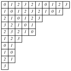
Figure 2. The $6$-core partition $\lambda=\mathcal{C}(w)=(10,9,6,5,5,3,2,2,2,1)$ for the minimal length coset representative $w=[-11,-9,-1,8,16,18]\in\widetilde{C}_{3}/C_{3}$. The numbers inside the boxes are the residues, described below.

Proposition 5.4.

The map $\mathcal{C}:\{\textup{abaci}\}\rightarrow\{\textup{partitions}\}$ is a bijection from and onto the sets shown in Table 4 on Page 4.

Proof.

A balanced flush abacus $a$ determines a partition $\mathcal{C}(a)$ by Definition 5.2. The fact that $a$ is flush by construction implies that $\mathcal{C}(a)$ is a $(2n)$-core. By Lemma 3.4, the sequence of gaps and beads is inverted when reflected about position $N$, so $\mathcal{C}(a)$ is symmetric.

We can define an inverse map. Starting from a $(2n)$-core partition $\lambda$, encode its southeast boundary lattice path on the abacus by recording each north-step as a bead and each east-step as a gap, placing the midpoint of the lattice path from $\lambda$ to lie between entries $N-1$ and $N+1$ on the abacus. The resulting abacus will be flush because $\lambda$ is a $(2n)$-core. The resulting abacus will be balanced because whenever position $i$ is the lowest bead on runner $(i\|N)$, then by symmetry $2N-i$ is the highest gap on runner $(N-i\|N)$ so $N-i$ is the lowest bead on runner $(N-i\|N)$.

Moreover, we claim that the map $\mathcal{C}$ restricts to a bijection between even abaci and even core partitions. In the correspondence between abaci and partitions, the entry $N$ corresponds to the midpoint of the boundary lattice path. In particular, this entry lies at the corner of a box on the main diagonal. Therefore, the number of gaps preceding $N$ in the reading order of $a$ is equal to the number of horizontal steps lying below the main diagonal of $\lambda=\mathcal{C}(a)$, which is exactly the number of boxes contained on the main diagonal of $\lambda$. ∎

5.2. Residues for the action of $\widetilde{W}$

If we translate the action of the Coxeter generators on abaci through the bijection $\mathcal{C}$, we obtain an action of $\widetilde{W}$ on the symmetric $(2n)$-core partitions.

To describe this action, we introduce the notion of a residue for a box in the diagram of a symmetric $(2n)$-core partition. The idea that motivates the following definitions is that $s_{i}$ should act on a symmetric $(2n)$-core $\lambda$ by adding or removing all boxes with residue $i$. In contrast with the situation in types $\widetilde{A}$ and $\widetilde{C}$, it will turn out that for types $\widetilde{B}$ and $\widetilde{D}$ the residue of a box in $\lambda$ may depend on $\lambda$ and not merely on the coordinates of the box.

To begin, we orient $\mathbb{N}^{2}$ so that $(i,j)$ corresponds to row $i$ and column $j$ of a partition diagram, and define the fixed residue of a position in $\mathbb{N}^{2}$ to be

$$\mathsf{res}(i,j)=\begin{cases}(j-i)\|(2n)&\text{ if }0\leq(j-i)\|(2n)\leq n\\ 2n-\big{(}(j-i)\|(2n)\big{)}&\text{ if }n<(j-i)\|(2n)<2n.\\ \end{cases}$$

Then, the fixed residues are given by extending the pattern illustrated below.

We define an escalator to be a connected component of the entries $(i,j)$ in $\mathbb{N}^{2}$ satisfying

$$(j-i)\|(2n)\in\{n-1,n,n+1\}.$$

If an escalator lies above the main diagonal $i=j$, then we say it is an upper escalator; otherwise, it is called a lower escalator. Similarly, we define a descalator to be a connected component of the entries $(i,j)$ in $\mathbb{N}^{2}$ satisfying

$$(j-i)\|(2n)\in\{-1,0,1\}.$$

If a descalator lies above the main diagonal $i=j$, then we say it is an upper descalator; if a descalator lies below the main diagonal $i=j$, it is called a lower descalator. There is one main descalator that includes the main diagonal $i=j$ which is neither upper nor lower.

Let $\lambda$ be a symmetric $(2n)$-core partition. We define the residues of the boxes in an upper escalator lying on row $i$ depending on the number of boxes in the $i$-th row of $\lambda$ that intersect the escalator, as shown in Figure 5.2(a).

(a)	(b)

Figure 3. Residue assignments for upper escalators and descalators

Here, the outlined boxes represent entries that belong to the row of $\lambda$, while the shaded cells represent entries in an upper escalator. The schematic in Figure 5.2(a) shows all ways in which these two types of entries can overlap, and we have written the residue assignments that we wish to assign for each entry.

Note that in the first case, where $\lambda$ is adjacent to but does not intersect the upper escalator, we view the first box of the escalator as being simultaneously $(n-1)$-addable and $n$-addable. In this case, the rightmost cell of the upper escalator has undetermined residue, and is neither addable nor removable. A similar situation occurs when a row of $\lambda$ ends with three boxes in the upper escalator. In all other cases, the entries of an upper escalator have undefined residue.

We similarly define the residues of the boxes in a lower escalator lying on column $j$ depending on the number of boxes in the $j$-th column of $\lambda$ that intersect the escalator. The precise assignment is simply the transpose of the schematic in Figure 5.2(a).

Moreover, we similarly define the residues of the boxes in an upper descalator on row $i$ depending on the number of boxes in the $i$-th row of $\lambda$ that intersect the descalator, as shown in Figure 5.2(b). The transpose of this schematic gives the assignment of residues of the boxes in a lower descalator.

Finally, the residues of the descalator containing the main diagonal are fixed, and we define the residue of an entry $(i,j)$ lying on the main descalator to be

$$\mathsf{mres}(i,j)=\begin{cases}0&\text{ if }(j-i)=0\\ 1&\text{ if }(j-i)\in\{1,-1\}\text{ and }(j+i)\equiv 1\mod 4\\ 0&\text{ if }(j-i)\in\{1,-1\}\text{ and }(j+i)\equiv 3\mod 4\\ \end{cases}$$

where the upper left most box has coordinates $(i,j)=(1,1)$.

Example 5.5.

In Figure 4, we consider residues using all of the features discussed above. It will turn out that this corresponds to type $\widetilde{D}_{5}/D_{5}$ and that the assignment of residues in each of the other types uses a subset of these features as described in the fourth column of Table 4.

Here, the unshaded entries of Figure 4 are fixed residues given by $\mathsf{res}(i,j)$ for $n=5$; the gray shaded entries represent an upper and lower escalator, and the blue shaded entries represent an upper and lower descalator. The descalator containing the main diagonal has fixed residues given by $\mathsf{mres}(i,j)$. The precise residues of the boxes in the upper/lower escalators/descalators for a particular partition depend on how the partition intersects the shaded regions.

Figure 4. The fixed residues in $\widetilde{D}_{5}/D_{5}$

Definition 5.6.

Suppose $\lambda$ is a symmetric $(2n)$-core partition representing an element of type $\widetilde{W}_{n}/W_{n}\in\{\widetilde{C}_{n}/C_{n},\widetilde{B}_{n}/B_{n},\widetilde{B}_{n}/D_{n},\widetilde{D}_{n}/D_{n}\}$, and embed the digram of $\lambda$ in $\mathbb{N}^{2}$ as above. Then we assign the residue of $(i,j)\in\mathbb{N}^{2}$ as described above, using the features listed in the fourth column of Table 4.

Type	Abaci	Partitions	Features for residue assignment
$\widetilde{C}/C$	balanced flush abaci	symmetric $(2n)$-cores	fixed residues only
$\widetilde{B}/B$	even balanced flush abaci	even symmetric $(2n)$-cores	fixed residues with descalators
$\widetilde{B}/D$	balanced flush abaci	symmetric $(2n)$-cores	fixed residues with escalators
$\widetilde{D}/D$	even balanced flush abaci	even symmetric $(2n)$-cores	fixed residues with escalators and descalators

Table 4. Core partitions for $\widetilde{W}/W$

Definition 5.7.

Given a symmetric $(2n)$-core partition $\lambda$ with residues assigned, we say that two boxes from $\mathbb{N}^{2}$ are $i$-connected whenever they share an edge and have the same residue $i$. We refer to the $i$-connected components of boxes from $\mathbb{N}^{2}$ as $i$-components.

We say that an $i$-component $C$ is addable if adding the boxes of $C$ to the diagram of $\lambda$ results in a partition, and that $C$ is removable if removing the boxes of $C$ from the diagram of $\lambda$ results in a partition.

We are now in a position to state the action of $\widetilde{W}$ on symmetric $(2n)$-core partitions in terms of residues.

Theorem 5.8.

Let $w\in\widetilde{W}/W$ and suppose $\lambda=\mathcal{C}(w)$. If $s_{i}$ is an ascent for $w$ then $s_{i}$ acts on $\lambda$ by adding all addable $i$-components to $\lambda$. If $s_{i}$ is a descent for $w$ then $s_{i}$ acts by removing all removable $i$-components from $\lambda$. If $s_{i}$ is neither an ascent nor a descent for $w$ then $s_{i}$ does not change $\lambda$.

The proof of this result is postponed to Section LABEL:s:proofs.

Example 5.9.

Consider the minimal length coset representative $w=[-12,-7,-5,2,3,8,9,16,18,23]\in\widetilde{D}_{5}/D_{5}$. The corresponding core partition $\lambda=\mathcal{C}(w)=(11,8,7,4,3,3,3,2,1,1,1)$ is pictured in Figure 5. The known residues are placed in their corresponding boxes.

If we were to apply the generator $s_{0}$ to $\lambda$, this would remove four boxes—the two boxes in the upper right corner and the two boxes in the lower left corner. The box on the main diagonal with residue $0$ is not removed because we cannot remove only part of its connected component of residue $0$ boxes.

From $\lambda$, we determine that $s_{0}$ and $s_{4}$ are descents (as they would remove boxes), $s_{1}$ and $s_{3}$ are ascents (as they would add boxes), and $s_{2}$ and $s_{5}$ are neither ascents nor descents (as they would leave the diagram unchanged).

Figure 5. The core partition $\lambda=\mathcal{C}(w)=(11,8,7,4,3,3,3,2,1,1,1)$ corresponding to the minimal length coset representative $w=[-12,-7,-5,2,3,8,9,16,18,23]\in\widetilde{D}_{5}/D_{5}$. The numbers indicate the residues of the boxes.

5.3. Bruhat order on symmetric $(2n)$-cores

In this section, we use an argument of Lascoux [lascoux-cores] to show that Bruhat order on the minimal length coset representatives $\widetilde{W}/W$ corresponds to a modified containment order on the corresponding core partition diagrams. This affirmatively answers a question of Billey and Mitchell [billey--mitchell, Remark 12].

Definition 5.10.

Let $\lambda$ and $\mu$ be two symmetric $(2n)$-cores. Suppose that every box of $\mu$ that does not lie on an escalator or descalator is also a box of $\lambda$, and that:

• Whenever the $i$-th row of $\mu$ intersects an upper escalator, upper descalator or the main descalator in $1$ box, then the $i$-th row of $\lambda$ intersects the given region in $1$ or $3$ boxes.

• Whenever the $i$-th row of $\mu$ intersects an upper escalator or upper descalator or the main descalator in $2$ boxes, then the $i$-th row of $\lambda$ intersects the given region in $2$ or $3$ boxes.

• Whenever the $i$-th row of $\mu$ intersects an upper escalator or upper descalator or the main descalator in $3$ boxes, then the $i$-th row of $\lambda$ intersects the given region in $3$ boxes.

In this situation, we say that $\lambda$ contains $\mu$, denoted $\lambda\unrhd\mu$.

Theorem 5.11.

Let $w,x\in\widetilde{W}/W$. Then $w\geq x$ in Bruhat order if and only if $\mathcal{C}(w)\unrhd\mathcal{C}(x)$.

Proof.

We proceed by induction on the number of boxes in $w$. When the Coxeter length of $w$ is $1$, then $x=w$, $x=e$, or $x$ is not related to $w$ in Bruhat order. In each case, the result is clear.

Let $s_{i}$ be a Coxeter generator such that $s_{i}w<w$ in $\widetilde{W}/W$. If $x\leq w$ then the Lifting Lemma [b-b, Proposition 2.2.7] implies that $s_{i}w\geq\min(x,s_{i}x)$ in $\widetilde{W}$. Every reduced expression for a nontrivial element of $\widetilde{W}/W$ ends in $s_{0}$, so if $s_{i}x<x$ then $s_{i}x\in\widetilde{W}/W$. Therefore, $s_{i}w\geq\min(x,s_{i}x)$ in $\widetilde{W}/W$.

Conversely, if $w>s_{i}w\geq\min(x,s_{i}x)$ in $\widetilde{W}/W$ then we find that $w\geq x$; this follows directly when $x<s_{i}x$ or $x=s_{i}x$, and follows by another application of the Lifting Lemma when $s_{i}x<x$.

We therefore have the equivalence $x\leq w$ if and only if $\min(x,s_{i}x)\leq s_{i}w$. Hence, we reduce to considering the pair $w^{\prime}=s_{i}w$, $x^{\prime}=\min(x,s_{i}x)$ in $\widetilde{W}/W$, and we need to show that $\mathcal{C}(w^{\prime})\unrhd\mathcal{C}(x^{\prime})$ if and only if $\mathcal{C}(w)\unrhd\mathcal{C}(x)$ to complete the proof by induction.

Suppose $\mathcal{C}(w)\unrhd\mathcal{C}(x)$. Then we pass to $\mathcal{C}(s_{i}w)$ by removing boxes with residue $i$ from the end of their rows and columns. By Definition 5.10, every such box from $\mathcal{C}(w)$ is either removable in $\mathcal{C}(x)$ or else absent from $\mathcal{C}(x)$. Hence, $\mathcal{C}(w^{\prime})\unrhd\mathcal{C}(x^{\prime})$. Similarly, it follows from Definition 5.10 that if $\mathcal{C}(w^{\prime})\unrhd\mathcal{C}(x^{\prime})$ then every addable box with residue $i$ in $\mathcal{C}(x^{\prime})$ is either addable in $\mathcal{C}(w^{\prime})$ or already present in $\mathcal{C}(w^{\prime})$. Hence, $\mathcal{C}(w)\unrhd\mathcal{C}(x)$. ∎

6. Reduced expressions from cores

6.1. The upper diagram

Let $\lambda=\mathcal{C}(w)$. We now define a recursive procedure to obtain a canonical reduced expression for $w$ from $\lambda$. Recall that the first diagonal is the diagonal immediately to the right of the main diagonal.

Definition 6.1.

Define the reference diagonal to be

$$\begin{cases}\text{the main diagonal }&\text{ in types $\widetilde{C}/C$ and $\widetilde{B}/D$ }\\ \text{the first diagonal }&\text{ in types $\widetilde{B}/B$ and $\widetilde{D}/D$ }\\ \end{cases}$$

Given a core $\lambda=\lambda^{(1)}$ we define the central peeling procedure recursively as follows. At step $i$, we consider $\lambda^{(i)}$ and set $d^{(i)}$ to be the number of boxes on the reference diagonal of $\lambda^{(i)}$. Suppose $B_{i}$ is the box at the end of the $d^{(i)}$-th row of $\lambda^{(i)}$ and $r_{i}$ is the residue of this box. In the case when $B_{i}$ is both $n$-removable and $(n-1)$-removable, we set $r_{i}=n$. Apply generator $s_{r_{i}}$ to $\lambda^{(i)}$ to find $\lambda^{(i+1)}$.

We define $\mathcal{R}(\lambda)$ to be the product of generators $s_{r_{1}}s_{r_{2}}\cdots s_{r_{\ell}}$.

We also define the upper diagram, denoted $U_{\lambda}$, to be the union of the boxes $B_{i}$ encountered in the central peeling procedure respecting the following conditions: In $\widetilde{B}/D$ and $\widetilde{D}/D$, the application of $s_{n}^{D}$ removes two boxes from the $d^{(i)}$-th row and we record in $U_{\lambda}$ the box not on the $n$-th diagonal; In $\widetilde{B}/B$ and $\widetilde{D}/D$, the application of $s_{0}^{D}$ removes two boxes from the $d^{(i)}$-th row and we record in $U_{\lambda}$ the box not on the main or $2n$-th diagonal.

Proposition 6.2.

We have that $\mathcal{R}(\lambda)$ is a reduced expression for $w$ and the number of boxes in $U_{\lambda}$ equals the Coxeter length of $\mathcal{W}(\lambda)$.

Proof.

At each step, the central peeling procedure records a descent so this follows from Proposition 5.8. ∎

We now present two examples of the central peeling procedure, one in $\widetilde{C}_{3}/C_{3}$ and another in $\widetilde{D}_{4}/D_{4}$.

Example 6.3.

The steps of the central peeling procedure applied to $\lambda=\mathcal{C}([-11,-9,-1,8,16,18])\in\widetilde{C}_{3}/C_{3}$ are presented in Figure 6. The collection of gray boxes tallied during the central peeling procedure is $U_{\lambda}$; Figure 7 shows $U_{\lambda}$ superimposed over $\lambda$. We can read off the canonical reduced expression $\mathcal{R}(\lambda)$ starting in the center of $\lambda$ and working our way up, reading the gray boxes from right to left. We have $\mathcal{R}(\lambda)=s_{0}s_{1}s_{0}s_{3}s_{2}s_{1}s_{0}s_{2}s_{3}s_{2}s_{1}s_{0}s_{2}s_{3}s_{2}s_{1}s_{0}$.

Example 6.4.

Let $w=[-15,-11,-10,4,5,19,20,24]\in\widetilde{D}_{4}/D_{4}$. The steps of the central peeling procedure applied to $\lambda=\mathcal{C}(w)$ are presented in Figure 8; notice that no tallied boxes are on the main diagonal or the fourth diagonal. These gray boxes make up $U_{\lambda}$, which in turn is superimposed over $\lambda$ in Figure 9. The canonical reduced expression is $\mathcal{R}(\lambda)=s_{0}s_{4}s_{2}s_{1}s_{4}s_{3}s_{2}s_{0}s_{4}s_{3}s_{2}s_{1}s_{4}s_{3}s_{2}s_{0}$.

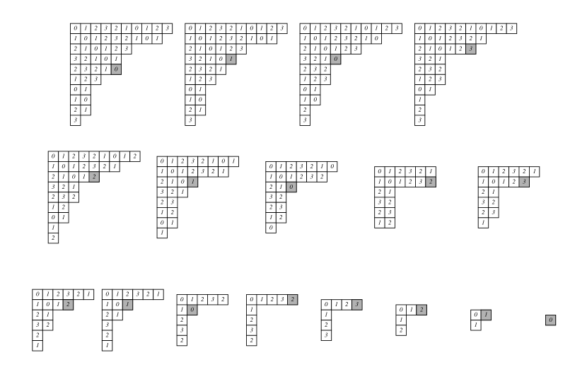
Figure 6. The application of the central peeling procedure described in Definition 6.1 on the core partition $\lambda=\mathcal{C}(w)$ for $w=[-11,-9,-1,8,16,18]\in\widetilde{C}_{3}/C_{3}$. The shaded boxes are the boxes $B_{i}$ tallied by the algorithm; they make up the upper diagram $U_{\lambda}$, shown in Figure 7.

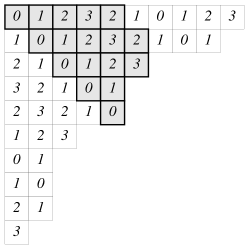
Figure 7. The core partition $\lambda=\mathcal{C}(w)$ for $w=[-11,-9,-1,8,16,18]\in\widetilde{C}_{3}/C_{3}$, with its upper diagram $U_{\lambda}$ superimposed. Reading the shaded boxes from the bottom to the top from right to left gives the canonical reduced expression $\mathcal{R}(\lambda)=s_{0}s_{1}s_{0}s_{3}s_{2}s_{1}s_{0}s_{2}s_{3}s_{2}s_{1}s_{0}s_{2}s_{3}s_{2}s_{1}s_{0}$.

Figure 8. The application of the central peeling procedure described in Definition 6.1 on the core partition $\lambda=\mathcal{C}(w)$ for $w=[-15,-11,-10,4,5,19,20,24]\in\widetilde{D}_{4}/D_{4}$. The shaded boxes are the boxes $B_{i}$ tallied by the algorithm; they make up the upper diagram $U_{\lambda}$, shown in Figure 9.

Figure 9. The core partition $\lambda=\mathcal{C}(w)$ for $w=[-15,-11,-10,4,5,19,20,24]\in\widetilde{D}_{4}/D_{4}$, with its upper diagram $U_{\lambda}$ shaded. ($U_{\lambda}$ was calculated in Figure 8.) Reading the shaded boxes from the bottom to the top from right to left gives the canonical reduced expression $\mathcal{R}(\lambda)=s_{0}s_{4}s_{2}s_{1}s_{4}s_{3}s_{2}s_{0}s_{4}s_{3}s_{2}s_{1}s_{4}s_{3}s_{2}s_{0}$.

6.2. The bounded diagram

We now describe a nonrecursive method to determine the upper diagram of any core $\lambda$. This method generalizes a bijection of Lapointe and Morse [LM] in $\widetilde{A}_{n}/A_{n}$.

We say that a box in $\lambda$ having hook length $<2n$ is skew. The skew boxes on any particular row form a contiguous segment lying at the end of the row. Consider the collection of boxes $\nu\subset\lambda$ defined row by row as the segment that begins at the box lying on the main diagonal and then extends to the right for the same number of boxes as the number of skew boxes in the row. In $\widetilde{B}/B$ and $\widetilde{D}/D$, remove from $\nu$ all boxes along the main diagonal. In $\widetilde{B}/D$ and $\widetilde{D}/D$, remove from $\nu$ all boxes along the $n$-th diagonal. We call this collection of boxes $\nu$ the bounded diagram of $\lambda$, denoted $\widetilde{U}_{\lambda}$.

Theorem 6.5.

Fix a symmetric $(2n)$-core partition $\lambda$. Then, the bounded diagram $\widetilde{U}_{\lambda}$ is equal to the upper diagram $U_{\lambda}$.

The proof of this theorem is postponed to Section LABEL:s:upper_partition.

Example 6.6.

For the minimal length coset representative $w=[-11,-9,-1,8,16,18]\in\widetilde{C}_{3}/C_{3}$ and its corresponding core partition $\lambda=\mathcal{C}(w)$, a visualization of the construction of $\widetilde{U}_{\lambda}$ is given in Figure 10. This agrees with $U_{\lambda}$ as found in Figure 7.

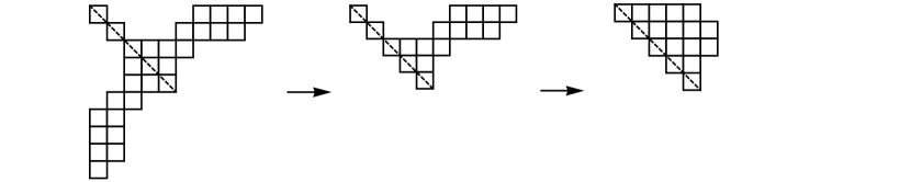
Figure 10. For $w=[-11,-9,-1,8,16,18]\in\widetilde{C}_{3}/C_{3}$, we left-justify the skew boxes to the boxes on the main diagonal to find the bounded diagram.

7. Bounded partitions

If we left-adjust the boxes of the upper diagram along with the residues they contain, we obtain a structure that has appeared in other contexts including: Young walls in crystal bases of quantum groups [HK], Eriksson and Eriksson’s partitions in [Erik2], the affine partitions of Billey and Mitchell [billey--mitchell], and the $k$-bounded partitions of Lapointe and Morse [LM]. Lam, Schilling and Shimozono [lam--schilling--shimozono] develop combinatorics analogous to the $k$-bounded partitions for type $\widetilde{C}$, and [spon] contains similar constructions for types $\widetilde{B}$ and $\widetilde{D}$. In this section, we explain how these objects are related to the abacus diagrams and core partitions we have introduced.

Definition 7.1.

Given a core $\lambda$, apply the central peeling procedure to find the upper diagram $U_{\lambda}$. We define the bounded partition $\mathcal{B}(\lambda)$ to be the partition $\beta$ whose $i$-th part equals the number of boxes in row $i$ of $U_{\lambda}$.

In $\widetilde{B}/D$ (and $\widetilde{D}/D$), if there exists a part of size $n$ ($n-1$, respectively), and the last part $\beta_{k}$ of this size has rightmost box with residue $n-1$, then adorn $\beta_{k}$ with a star decoration.

By construction, the number of boxes in a bounded partition is the Coxeter length of the corresponding element in $\widetilde{W}/W$. Besides being historical, the motivation for the name “bounded partition” is that part sizes in $\mathcal{B}(w)$ are bounded in the different types by $2n$, $2n-1$, or $2n-2$, as shown in Table LABEL:t:bdd.

Remark 7.2.

The need for a decoration in $\widetilde{B}/D$ and $\widetilde{D}/D$ arises because it is possible that two core partitions yield the same bounded partition. For example, consider elements $w_{1}=s_{0}s_{1}\cdots s_{n-2}s_{n-1}$ and $w_{2}=s_{0}s_{1}\cdots s_{n-2}s_{n}$ of $\widetilde{B}/D$. They both have the same Coxeter length and correspond to a bounded partition with one part of size $n$; however, these elements are distinct and have different abaci and cores. We would say that $\mathcal{B}(w_{1})=(n^{*})$ and $\mathcal{B}(w_{2})=(n)$. The reader should interpret the star as arising from a length $n$ sequence of generators (length $n-1$ in type $\widetilde{D}/D$) that ends with $s_{n-1}$ instead of $s_{n}$.

Recall that Definition 5.2 gives a correspondence between rows of $\lambda$ and active beads in $\mathcal{A}(\lambda)$. Together with Theorem 6.5, this presents a method to determine the bounded partition from an abacus diagram.

Lemma 7.3.

For a row $r$ of $\lambda$ corresponding to an active bead $b>N$ in $\mathcal{A}(\lambda)$, the number of skew boxes in row $r$ on or above the main diagonal equals the number of gaps between $b$ and $\max(b-N,g(b))$, inclusive.

Proof.

By definition 5.2, the skew boxes on a row corresponding to an active bead $b$ are the gaps between $b-N$ and $b$. Also, the diagonal box on this row corresponds to the symmetric gap $g(b)$, and the result follows. ∎

Define offsets $x_{0}$ and $x_{n}$ corresponding to the occurrence of generators $s_{0}^{D}$ and $s_{n}^{D}$ as follows. These offsets record whether a fork occurs on the left or right sides of the Coxeter graph, respectively. x_0=