Performance of mutual information inference methods under unknown interference

Abstract

In this paper, the problem of fast point-to-point MIMO channel mutual information estimation is addressed, in the situation where the receiver undergoes unknown colored interference, whereas the channel with the transmitter is perfectly known. The considered scenario assumes that the estimation is based on a few channel use observations during a short sensing period. Using large dimensional random matrix theory, an estimator referred to as G-estimator is derived. This estimator is proved to be consistent as the number of antennas and observations grow large and its asymptotic performance is analyzed. In particular, the G-estimator satisfies a central limit theorem with asymptotic Gaussian fluctuations. Simulations are provided which strongly support the theoretical results, even for small system dimensions.

I Introduction

The use of multiple-input-multiple-output (MIMO) technologies has the potential to achieve high data rates, since several independent channels between the transmitter and the receiver can be exploited. However, the proper evaluation of the achievable rate in the MIMO setting is fundamentally contingent to the knowledge of the transmit-receive channel as well as of the interference pattern. In recent communication schemes such as cognitive radios [1], it is fundamental for a receiver to be able to infer these achievable rates in a short sensing period, hence extremely fast. This article is dedicated to the study of novel algorithms that partially fulfill this task without resorting to the (usually time consuming) evaluation of the covariance matrix of the interference.

Conventional methods for the estimation of the mutual information in single antenna systems rely on the use of classical estimation techniques which assume a large number of observations. In general, consider $\theta$ a parameter we wish to estimate, and $M$ the number of independent and identically distributed (i.i.d.) observation vectors ${\bf y}_{1},\cdots,{\bf y}_{M}\in{\mathbb{C}}^{N}$. Assume $\theta$ is a function of the covariance matrix ${\bm{\Sigma}}=\mathbb{E}\left[{\bf y}_{1}{\bf y}_{1}^{{\sf H}}\right]$ of the received random process, i.e. $\theta=f({\bm{\Sigma}})$, for some function $f$. From the strong law of large numbers, a consistent estimate of the covariance of the random process is simply given by the empirical covariance of ${\bf Y}=\left[{\bf y}_{1},\cdots,{\bf y}_{M}\right]$, i.e. $\widehat{\bm{\Sigma}}\triangleq\frac{1}{M}{\bf Y}{\bf Y}^{{\sf H}}=\frac{1}{M}\sum_{i=1}^{M}{\bf y}_{i}{\bf y}_{i}^{{\sf H}}$. The one-step estimator $\widehat{\theta}$ of $\theta$ would then consist in using the empirical covariance matrix $\widehat{\bm{\Sigma}}$ as a good approximation of ${\bm{\Sigma}}$, thus yielding $\widehat{\theta}=f(\widehat{\bm{\Sigma}})$ [2]. Such methods provide good performance as long as the number of observations $M$ is very large compared to the vector size $N$, a situation not always encountered in wireless communications, especially in fast changing channel environments.

To address the scenario where the number of observations $M$ is of the same order as the dimension $N$ of each observation, new consistent estimation methods, sometimes called G-estimation methods (named after Girko’s pioneering works [3, 4] on General Statistical Analysis) have been developed, mainly based on large dimensional random matrix theory. In the context of wireless communications, works devoted to the estimation of eigenvalues and eigenspace projections [5, 6] have given rise to improved subspace estimation techniques [7, 8]. Recently, the use of these methods to better estimate system performance indexes in wireless communications has triggered the interest of many researchers. In particular, the estimation of the mutual information of MIMO systems under imperfect channel knowledge has been addressed in [9] and [10], where methods based respectively on free probability theory and the Stieltjes transform were proposed.

In this article, we consider a different situation where the receiver perfectly knows the channel with the transmitter but does not a priori know the experienced interference. Such a situation can be encountered in multi-cell scenarios, where interference stemming from neighboring cell users changes fast, which is a natural assumption in packet switch transmissions. Our target is to estimate the instantaneous or ergodic mutual information of the transmit-receive link, which serves here as an approximation of the achievable communication rate provided that no improved precoding is performed. An important usage of the mutual information estimation is found in the context of cognitive radios where multiple frequency bands are sensed for future transmissions. In this setting, the proposed estimator provides the expected rate performance (either instantaneous or ergodic) achievable in each frequency band, prior to actual transmission. The transmit-receive pair may then elect the frequency sub-bands most suitable for communication.

The setting of the article assumes that the channel from the transmitter to the receiver is known by the receiver (but not known by the transmitter), which is a realistic scenario provided that some channel state feedback is delivered by the transmitter, and that the statistical inference on the mutual information is based on $M$ successive observations of channel uses, where $M$ is not large compared to the number of receive antennas $N$, therefore naturally calling for the G-estimation framework. The progression of this article will consist first in studying the conventional one-step estimator, hereafter called the standard empirical (SE) estimator, which corresponds to estimating the interference covariance matrix by the empirical covariance matrix and to replacing the estimate in the mutual information formula. We then show that this approach, although consistent in the large $M$ regime, performs poorly in the regime where both $M$ and $N$ are of similar sizes. We then provide an alternative approach, based on the G-estimation scheme, and produce a novel G-estimator of the mutual information which we first prove consistent in the large $M,N$ regime and for which we derive the asymptotic second order performance through a central limit theorem.

The remainder of the article is structured as follows. In Section II, the system model is described and the considered problem is mathematically formalized. In Section III, first order results for both the SE-estimator and the G-estimator are provided. In Section IV, the fluctuations of the G-estimator are studied. We then provide in Section V numerical simulations that support the accuracy of the derived results, before concluding the article in Section VI. Mathematical details are provided in the appendices.

Notations

In the following, boldface lower case symbols represent vectors, capital boldface characters denote matrices (${\bf I}_{N}$ is the size-$N$ identity matrix). If ${\bf A}$ is a given matrix, ${\bf A}^{{\sf H}}$ stands for its transconjugate; if ${\bf A}$ is square, $\operatorname{tr}({\bf A})$, $\det({\bf A})$ and $\|{\bf A}\|$ respectively stand for the trace, the determinant and the spectral norm of ${\bf A}$. We say that the variable $X$ has a standard complex Gaussian distribution if $X=U+\mathbf{i}V$ ($\mathbf{i}^{2}=-1$) , where $U,V$ are independent real random variables with Gaussian distribution ${\mathcal{N}}(0,1/2)$. The complex conjugate of a scalar $z$ will be denoted by $z^{*}$. Almost sure convergence will be denoted by $\xrightarrow[]{\textrm{a.s.}}$, and convergence in distribution by $\xrightarrow[]{\mathcal{D}}$. Notation ${\mathcal{O}}$ will refer to Landau’s notation: $u_{n}={\mathcal{O}}(v_{n})$ if there exists a bounded sequence $K_{n}$ such that $u_{n}=K_{n}v_{n}$. For a square $N\times N$ Hermitian matrix $\bf A$, we denote $\lambda_{1}({\bf A})\leq\ldots\leq\lambda_{N}({\bf A})$ the ordered eigenvalues of $\bf A$.

II System model and problem setting

II-A System model

Consider a wireless communication channel ${\bf H}_{t}\in{\mathbb{C}}^{N\times n_{0}}$ between a transmitter equipped with $n_{0}$ antennas and a receiver equipped with $N$ antennas, the latter being exposed to interfering signals. The objective of the receiver is to evaluate the mutual information of this link during a sensing period assuming ${\bf H}_{t}$ known at all time. For this, we assume a block-fading scenario and denote by $T\geq 1$ the number of channel coherence intervals (or time slots) allocated for sensing. In other words, we suppose that, within each channel coherence interval $t\in\{1,\ldots,T\}$, ${\bf H}_{t}$ is deterministic and constant. We also denote by $M$ the number of channel uses employed for sensing during each time slot ($M$ times the channel use duration is therefore less than the channel coherence time). The $M$ concatenated signal vectors received in slot $t$ are gathered in the matrix $\overline{{\bf Y}}_{t}\in{\mathbb{C}}^{N\times M}$ defined as

$$\overline{{\bf Y}}_{t}={\bf H}_{t}{\bf X}_{t,0}+\overline{{\bf W}}_{t}$$

where ${\bf X}_{t,0}\in{\mathbb{C}}^{n_{0}\times M}$ is the concatenated matrix of the transmitted signals and $\overline{{\bf W}}_{t}\in{\mathbb{C}}^{N\times M}$ represents the concatenated interference vectors.

Since $\overline{{\bf W}}_{t}$ is not necessarily a white noise matrix in the present scenario, we write $\overline{{\bf W}}_{t}={\bf G}_{t}{\bf W}_{t}$ where ${\bf G}_{t}\in{\mathbb{C}}^{N\times n}$ is such that ${\bf G}_{t}{\bf G}_{t}^{\sf H}\in{\mathbb{C}}^{N\times N}$ is the deterministic matrix of the noise variance during slot $t$ while ${\bf W}_{t}\in{\mathbb{C}}^{n\times M}$ is a matrix filled with independent entries with zero mean and unit variance. That is, we assume that the interference is stationary during the coherence time of ${\bf H}_{t}$, which is a reasonable assumption in practical scenarios, as commented in Remark 1. The choice of using the additional system parameter $n$, not necessarily equal to $N$, is also motivated by practical applications where the sources of interference may be of different dimensionality than the number of receive antennas, as discussed in Remark 1 below. This will have no effect on the resulting mutual information estimators.

We finally assume that perfect decoding of ${\bf X}_{t,0}$ (possibly transmitted at low rate or not transmitted at all) is achieved during the sensing period. If so, since ${\bf H}_{t}$ is assumed perfectly known, the residual signal to which the receiver has access is given by

$${\bf Y}_{t}=\overline{{\bf Y}}_{t}-{\bf H}_{t}{\bf X}_{t,0}={\bf G}_{t}{\bf W}_{t}.$$

Remark 1

The usual white noise assumption naturally arises from the thermal noise created by the electronic components at the receiver radio front end as well as from the large number of exogenous sources of interference in the vicinity of the receiver. However, in cellular networks, and particularly so in cell edge conditions, the main source of interference arises from coherent transmissions in adjacent cells. In this case, only a small number $K$ of signal sources interfere in a colored manner. Calling ${\bf G}_{t,k}\in{\mathbb{C}}^{N\times n_{k}}$ the channel from interferer $k\in\{1,\ldots,K\}$, equipped with $n_{k}$ antennas, to the receiver and ${\bf X}_{t,k}\in{\mathbb{C}}^{n_{k}\times M}$ the concatenated transmit signals from interferer $k$, the received signal $\overline{{\bf Y}}_{t}$ can be modeled as

$$\overline{{\bf Y}}_{t}={\bf H}_{t}{\bf X}_{t,0}+\sum_{k=1}^{K}{\bf G}_{t,k}{\bf X}_{t,k}+\sigma{\bf W}^{\prime}_{t}$$ (1)

where $\sigma{\bf W}^{\prime}_{t}\in{\mathbb{C}}^{N\times M}$ is the concatenated additional white Gaussian noise with variance $\sigma^{2}>0$. In this case, we see that, denoting $n=n_{1}+\ldots+n_{K}+N$ and

$${\bf G}_{t} =\left[{\bf G}_{t,1},\cdots,{\bf G}_{t,K},\sigma{\bf I}_{N}\right]$$

$${\bf W}_{t} =\left[{\bf X}_{t,1}^{{\sf T}},\cdots,{\bf X}_{t,K}^{{\sf T}},{{\bf W}^{\prime}_{t}}^{{\sf T}}\right]^{{\sf T}}$$

we fall back on the above model. Figure 1 depicts this scenario in the case of $K=2$ interfering users.

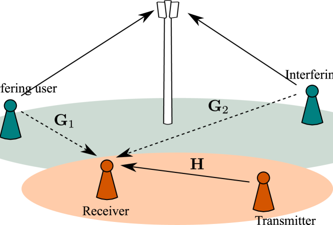
Figure 1: System model of Remark 1 with two interferers.

The statistical properties of the random variables ${\bf X}_{t,0}$ and ${\bf W}_{t}$ are precisely described as follows.

Assumption A1

For a given $t$ where $1\leq t\leq T$, the entries of the matrices ${\bf X}_{t,0}$ and ${\bf W}_{t}$ are i.i.d. random variables with standard complex Gaussian distribution.

The objective for the receiver is to evaluate the average (per-antenna) mutual information that can be achieved during the $T$ slots. In particular, for $T=1$, the expression is that of the instantaneous mutual information which allows for an estimation of the rate performance of the current channel. If $T$ is large instead, this provides an approximation of the long-term ergodic mutual information. Under Assumption A1, the average mutual information is given by

$${\mathcal{I}} = \frac{1}{NT}\sum_{t=1}^{T}\left[\log\det\left({\bf H}_{t}{\bf H}_{t}^{{\sf H}}+{\bf G}_{t}{\bf G}_{t}^{\sf H}\right)-\log\det\left({\bf G}_{t}{\bf G}_{t}^{\sf H}\right)\right].$$ (2)

The target of the article is to address the problem of estimating ${\mathcal{I}}$ based on $T$ successive observations ${\bf Y}_{1},\ldots,{\bf Y}_{T}$ assuming perfect knowledge of ${\bf H}_{1},\cdots,{\bf H}_{T}$, but unknown ${\bf G}_{t}$ for all $t$.

II-B The standard empirical estimator $\hat{\mathcal{I}}_{\mathrm{SE}}$

If the number $M$ of available observations during the sensing period in each slot is very large compared to the channel vector $N$, a natural estimator, hereafter referred to as the standard empirical (SE) estimator, consists in the following one-step estimator

$$\hat{\mathcal{I}}_{\mathrm{SE}}\quad=\quad\frac{1}{NT}\sum_{t=1}^{T}\log\det\left({\bf H}_{t}{\bf H}_{t}^{{\sf H}}+\frac{1}{M}{\bf Y}_{t}{\bf Y}_{t}^{{\sf H}}\right)-\frac{1}{NT}\sum_{t=1}^{T}\log\det\left(\frac{1}{M}{\bf Y}_{t}{\bf Y}_{t}^{{\sf H}}\right)\ .$$ (3)

For future use, it is convenient to introduce the notation

$$\hat{\mathcal{I}}_{\mathrm{SE}}(y) = \frac{1}{NT}\sum_{t=1}^{T}\log\det\left(y\,{\bf H}_{t}{\bf H}_{t}^{{\sf H}}+\frac{1}{M}{\bf Y}_{t}{\bf Y}_{t}^{{\sf H}}\right)-\frac{1}{NT}\sum_{t=1}^{T}\log\det\left(\frac{1}{M}{\bf Y}_{t}{\bf Y}_{t}^{{\sf H}}\right)\ .$$ (4)

With this notation at hand, $\hat{\mathcal{I}}_{\mathrm{SE}}=\hat{\mathcal{I}}_{\mathrm{SE}}(1)$.

For $N$ fixed, it is an immediate application of the law of large numbers and of the continuous mapping theorem to observe that, as $M\to\infty$,

$$\hat{\mathcal{I}}_{\mathrm{SE}}-{\mathcal{I}}\overset{\rm a.s.}{\longrightarrow}0.$$ (5)

However, from the discussions above, the assumption $M\gg N$ may not be tenable for practical settings where sensing needs to be performed fast, particularly so under fast fading conditions. In this case, as will be shown in Section III, the SE-estimator is asymptotically biased in the large $M,N$ regime, hence not consistent, and (5) will no longer hold true. This motivates the study of an alternative consistent estimator based on the G-estimation framework. To this end, we first need to study in depth the statistical properties of the SE-estimator from which the G-estimator will naturally arise. The statistical properties of the latter will similarly be obtained by first studying the second order statistics of the SE-estimator (themselves being of limited practical interest). Before moving to our main results, we first need some further technical hypotheses.

II-C The asymptotic regime

In this section, we formalize the conditions under which the large $M,N$ regime is considered. We will require the following assumptions.

Assumption A2

$M,N,n,n_{0}\to+\infty$, and

$$0 < \liminf_{M,N\rightarrow\infty}\frac{N}{n}\quad\leq\quad\limsup_{M,N\rightarrow\infty}\frac{N}{n}\ <\ +\infty\ ,$$

$$1 < \liminf_{M,N\rightarrow\infty}\frac{M}{N}\quad\leq\ \quad\limsup_{M,N\rightarrow\infty}\frac{M}{N}\ <\ +\infty\ ,$$

$$0 < \liminf_{N,n_{0}\rightarrow\infty}\frac{n_{0}}{N}\quad\leq\quad\limsup_{N,n_{0}\rightarrow\infty}\frac{n_{0}}{N}\ <\ +\infty\ .$$

Remark 2

The constraints over $N$ and $n$ simply state that these quantities remain of the same order. The lower bound for the ratio $M/N$ accounts for the fact that that $M$ is larger than $N$, although of the same order.

In the remainder of the article, we may refer to Assumption A2 as the convergence mode $M,N,n\to\infty$.

We also need the channel matrices to be bounded in spectral norm, as $M,N,n\to\infty$, as follows.

Assumption A3

Let $N=N(n)$ a sequence of integers indexed by $n$. For each $t\in\left\{1,\cdots,T\right\}$, consider the family of $N\times n$ matrices ${\bf G}_{t}$. Then,

• The spectral norms of ${\bf G}_{t}$ are uniformly bounded in the sense that

  $$\sup_{1\leq t\leq T}\sup_{N,n}\|{\bf G}_{t}\|<\infty\ .$$

• For $t\in\{1,\cdots,T\}$, the smallest eigenvalue of ${\bf G}_{t}{\bf G}_{t}^{\sf H}$ denoted by $\lambda_{N}({\bf G}_{t}{\bf G}_{t}^{\sf H})$ is uniformily bounded away from zero, i.e. there exists $\sigma^{2}>0$ such that

  $$\inf_{1\leq t\leq T}\inf_{N,n}\lambda_{N}({\bf G}_{t}{\bf G}_{t}^{\sf H})\geq\sigma^{2}>0\ .$$

Assumption A4

Let $N=N(n_{0})$ a sequence of integers indexed by $n_{0}$. For each $t\in\left\{1,\cdots,T\right\}$, consider the family of $N\times n_{0}$ matrices ${\bf H}_{t}$. Then, The spectral norms of ${\bf H}_{t}$ are uniformly bounded in the sense that

$$\sup_{1\leq t\leq T}\sup_{N,n_{0}}\|{\bf H}_{t}\|<\infty\ .$$

Assumption A5

The family of matrices $({\bf H}_{t})$ satisfies additionally the following assumptions:

• Denote by $p_{t}$ the rank of ${\bf H}_{t}$. Then

  $$0\ <\ \liminf_{N,n_{0}\rightarrow\infty}\frac{p_{t}}{N}\ \leq\ \limsup_{N,n_{0}\rightarrow\infty}\frac{p_{t}}{N}\ <\ 1\ .$$

• The smallest non-zero eigenvalue of ${\bf H}_{t}{\bf H}_{t}^{{\sf H}}$ is uniformly bounded away from zero, i.e. there exists $\kappa>0$ such that:

  $$\inf_{1\leq t\leq T}\inf_{N,n_{0}}\left\{\lambda_{i}({\bf H}_{t}{\bf H}_{t}^{{\sf H}})~{}|~{}\lambda_{i}({\bf H}_{t}{\bf H}_{t}^{{\sf H}})>0\right\}\geq\kappa>0.$$

III Convergence of the average mutual information estimators

In this section, we study the asymptotic behavior of the SE-estimator $\hat{\mathcal{I}}_{\mathrm{SE}}$ and prove that under the asymptotic regime A2, this estimator is asymptotically biased. Relying on this first analysis, we then derive a consistent estimator based on the random matrix inference techniques known as G-estimation.

These techniques can be classified in two categories. One is based on the link between the Stieltjes transform (see Appendix A) and the Cauchy complex integral, recently exhibited by Mestre who developed a framework for the estimation of eigenvalues and eigenspace projections [5]. This approach is often well-adapted as long as the estimation of parameters depending either on the eigenvalues or on the eigenvector projections of ${\bf Y}_{t}{\bf Y}_{t}^{\sf H}$ is considered (see for instance Lemma 1) but may fail when the dependence is more involved. The second approach, which we will adopt here, is based on the technique of deterministic equivalents developed in [11, 12]. It follows from the initial work [10] of Vallet and Loubaton, and will be illustrated in Section III-B.

III-A The standard empirical estimator $\hat{\mathcal{I}}_{\mathrm{SE}}$

We start by studying the second of the two terms in the difference (2) for which it is much easier to derive an estimate.

Lemma 1

Let Assumptions A1-A4 hold. Then, we have the following convergence.

$$\frac{1}{N}\log\det({\bf G}_{t}{\bf G}_{t}^{{\sf H}})-\frac{1}{N}\log\det\left(\frac{1}{M}{\bf Y}_{t}{\bf Y}_{t}^{{\sf H}}\right)+\frac{N-M}{N}\log\left(\frac{M-N}{M}\right)-1\xrightarrow[M,N,n\rightarrow\infty]{\textrm{a.s.}}0\ .$$

Proof:

See Appendix A ∎

Remark 3

It should be noted that in the proof of lemma 1, the Gaussianity assumption of the entries is not necessary and can be replaced by a finite moment condition.

Remark 4

Lemma 1 relies on the Stieltjes transform estimation technique from Mestre. The latter is used to compute a consistent estimate of the quantity $\frac{1}{N}\sum_{t=1}^{T}\log\det({\bf G}_{t}{\bf G}_{t}^{{\sf H}})$, which is seen here as a functional of the (non-observable) eigenvalues of ${\bf G}_{t}{\bf G}_{t}^{\sf H}$. Following the work from Mestre [5], the idea is to link the Stieltjes transform of ${\bf G}_{t}{\bf G}_{t}^{\sf H}$ to that of the (almost sure) limiting Stieltjes transform of the (observable) sample covariance matrix $\frac{1}{M}{\bf Y}_{t}{\bf Y}_{t}^{{\sf H}}$. See [13] for a tutorial on these notions.

As a consequence of Lemma 1, we see that the $\frac{1}{N}\log\det(\frac{1}{M}{\bf Y}_{t}{\bf Y}_{t}^{{\sf H}})$ is a consistent estimate of $\frac{1}{N}\log\det({\bf G}_{t}{\bf G}_{t}^{{\sf H}})$ (recall that $\frac{1}{M}\mathbb{E}{{\bf Y}}_{t}{{\bf Y}}_{t}^{{\sf H}}={\bf G}_{t}{\bf G}_{t}^{{\sf H}}$) up to a bias term depending on the time and space dimensions only. This may suggest that, up to the introduction of the term ${\bf H}_{t}{\bf H}_{t}^{{\sf H}}$ in the log determinants for estimating the first term in (2), the SE-estimator is also a consistent estimator for ${\mathcal{I}}$. This is however not true. To study the first term in (2), which is not as immediate as the second term, we need some further work. We start with a first technical lemma which follows instead from random matrix operations on deterministic equivalents.

Lemma 2

Let Assumptions A1–A4 hold and let $y>0$. Then we have the following identities.

1. The fixed-point equation in $y$

   $$\kappa_{t}(y)=\frac{1}{M}\operatorname{tr}\left({\bf G}_{t}{\bf G}_{t}^{\sf H}\left(\frac{{\bf G}_{t}{\bf G}_{t}^{\sf H}}{1+\kappa_{t}(y)}+y{\bf H}_{t}{\bf H}_{t}^{{\sf H}}\right)^{-1}\right)$$ (6)

   admits a unique positive solution $\kappa_{t}(y)$.

Denote by ${\bf T}_{t}(y)$ and ${\bf Q}_{t}(y)$ the following quantities:

$${\bf T}_{t}(y)=\left(y{\bf H}_{t}{\bf H}_{t}^{{\sf H}}+\frac{{\bf G}_{t}{\bf G}_{t}^{\sf H}}{1+\kappa_{t}(y)}\right)^{-1}\ ,\quad{\bf Q}_{t}(y)=\left(y{\bf H}_{t}{\bf H}_{t}^{{\sf H}}+\frac{1}{M}{\bf Y}_{t}{\bf Y}_{t}^{{\sf H}}\right)^{-1}\ .$$

1. Then, for any deterministic family $({\bf S}_{N})$ of $N\times N$ complex matrices with uniformly bounded spectral norm, we have:

   $$\frac{1}{M}\operatorname{tr}{\bf S}_{N}{\bf Q}_{t}(y)-\frac{1}{M}\operatorname{tr}{\bf S}_{N}{{\bf T}}_{t}(y)\xrightarrow[M,N,n\rightarrow\infty]{\textrm{a.s.}}0.$$

2. Let

   $$V_{t}(y)=\log\det\left(y{\bf H}_{t}{\bf H}_{t}^{{\sf H}}+\frac{{\bf G}_{t}{\bf G}_{t}^{\sf H}}{1+\kappa_{t}(y)}\right)+M\log(1+\kappa_{t}(y))-M\frac{\kappa_{t}(y)}{1+\kappa_{t}(y)}.$$

   Then, the following convergence holds

   $$\frac{1}{N}\log\det\left(y{\bf H}_{t}{\bf H}_{t}^{{\sf H}}+\frac{1}{M}{\bf Y}_{t}{\bf Y}_{t}^{{\sf H}}\right)-\frac{1}{N}V_{t}(y)\xrightarrow[M,N,n\rightarrow\infty]{\textrm{a.s.}}0\ .$$

Proof:

See Appendix B. ∎

Clearly, when setting $y=1$, this result provides a convergence result for the SE-estimator, as will be stated in Theorem 1. Lemma 2 is however more generic in its replacing the term $1$ in front of ${\bf H}_{t}{\bf H}_{t}^{\sf H}$ by an auxiliary parameter $y$. As a matter of fact, the introduction of $y$ is at the core of the novel estimator derived later. We can indeed already anticipate the remainder of the derivations: if $(1+\kappa_{t}(y))^{-1}$ can be made equal to $y$, then the first term in the expression of $V_{t}(y)$ is proportional to the first term in (2) which we are interested in. Turning the factor $1$ into a generic variable $y$ will therefore provide the flexibility missing to estimate (2) precisely in the large $M,N,n$ regime. Before getting into these considerations, let us start with the following result on the SE-estimator.

Theorem 1 (Asymptotic bias of the SE-estimator)

Let Assumptions A1-A4 hold, and denote

$$\mathcal{V}(y) =\frac{1}{NT}\sum_{t=1}^{T}\left(\log\det\left(y{\bf H}_{t}{\bf H}_{t}^{{\sf H}}+\frac{{\bf G}_{t}{\bf G}_{t}^{\sf H}}{1+\kappa_{t}(y)}\right)-\log\det({\bf G}_{t}{\bf G}_{t}^{{\sf H}})\right)$$

$$+\frac{1}{T}\sum_{t=1}^{T}\left(\frac{M}{N}\log(1+\kappa_{t}(y))-\frac{M}{N}\frac{\kappa_{t}(y)}{1+\kappa_{t}(y)}\right)+\frac{M-N}{N}\log\left(\frac{M-N}{M}\right)+1.$$ (7)

where $\kappa_{t}(y)$ is the unique solution of (6). Then,

$$\hat{\mathcal{I}}_{\mathrm{SE}}-\mathcal{V}(1)\xrightarrow[M,N,n\rightarrow\infty]{\textrm{a.s.}}0\ .$$

Proof:

Gathering item 3) of Lemma 2 together with Lemma 1 yields the desired result. ∎

This result suggests that the SE-estimator is not necessarily a consistent estimator of the mutual information, as there is no reason for the bias term in (1) (for $y=1$) to be identically null. However, based on the discussion prior to Theorem 1, we are now in position to derive a novel consistent estimator. The following section is dedicated to this task.

III-B A G-estimator of the average mutual information

The following result is our main contribution, which provides the novel consistent estimator for (2).

Theorem 2 (G-estimator for the average mutual information)

Assume that A1-A4 hold and define the quantity

$$\hat{\mathcal{I}}_{\mathrm{G}} =\frac{1}{NT}\sum_{t=1}^{T}\log\det\left({\bf I}_{N}+\hat{y}_{N,t}{\bf H}_{t}{\bf H}_{t}^{{\sf H}}\left(\frac{1}{M}{\bf Y}_{t}{\bf Y}_{t}^{{\sf H}}\right)^{-1}\right)$$

$$+\frac{1}{T}\sum_{t=1}^{T}\frac{(M-N)}{N}\left[\log\left(\frac{M}{M-N}\hat{y}_{N,t}\right)+1\right]-\frac{M}{N}\hat{y}_{N,t}$$

where $\hat{y}_{N,t}$ is the unique real positive solution of

$$\hat{y}_{N,t}=\frac{\hat{y}_{N,t}}{M}\operatorname{tr}{\bf H}_{t}{\bf H}_{t}^{{\sf H}}\left(\hat{y}_{N,t}\,{\bf H}_{t}{\bf H}_{t}^{{\sf H}}+\frac{1}{M}{\bf Y}_{t}{\bf Y}_{t}^{{\sf H}}\right)^{-1}+\frac{M-N}{M}.$$

Then

$$\hat{\mathcal{I}}_{\mathrm{G}}-{\mathcal{I}}\xrightarrow[M,N,n\rightarrow\infty]{\textrm{a.s.}}0\ .$$

Proof:

We hereafter provide an outline of the proof, which is developed in full detail in Appendix C. Denote ${\mathcal{I}}_{t}$ the average mutual information at time $t$ as

$${\mathcal{I}}_{t} \triangleq \frac{1}{N}\log\det({\bf G}_{t}{\bf G}_{t}^{{\sf H}}+{\bf H}_{t}{\bf H}_{t}^{{\sf H}})-\frac{1}{N}\log\det({\bf G}_{t}{\bf G}_{t}^{{\sf H}})\ ,$$

$$\triangleq {\mathcal{I}}_{t,1}-{\mathcal{I}}_{t,2}.$$

Recall that a consistent estimate $\hat{\mathcal{I}}_{t,2}$ of ${\mathcal{I}}_{t,2}$ was provided in Lemma 1. It therefore remains to build a consistent estimate for ${\mathcal{I}}_{t,1}$.

The proof is divided into four steps, as follows.

1. In the first step, we exploit the convergence of parametrized quantities of interest. Denote

   $$f(y)=\frac{1}{N}\log\det\left(\frac{1}{M}{\bf Y}_{t}{\bf Y}_{t}^{{\sf H}}+y{\bf H}_{t}{\bf H}_{t}^{{\sf H}}\right)$$

   and recall the definition of $\kappa_{t}(y)$ as given in Lemma 2-1). By Lemma 2-3),

   $$-f(y)+\frac{1}{N}\log\det\left(\frac{{\bf G}_{t}{\bf G}_{t}^{{\sf H}}}{1+\kappa_{t}(y)}+y{\bf H}_{t}{\bf H}_{t}^{{\sf H}}\right)+\frac{M}{N}\log(1+\kappa_{t}(y))-\frac{M}{N}\frac{\kappa_{t}(y)}{1+\kappa_{t}(y)}\xrightarrow[M,N,n\rightarrow\infty]{\mathrm{a.s}}0\ .$$

   Clearly, for most values of $y$; the deterministic quantity to which $f(y)$ converges differs from ${\mathcal{I}}_{t,1}$.

2. In the second step, we find a specific value of $y$ to enforce the desired quantity ${\mathcal{I}}_{t,1}$ to appear. One can readily check that if $y_{N,t}$ is the solution of the equation in $y$

   $$y=\frac{1}{1+\kappa_{t}(y)}$$ (8)

   then we immediately obtain

   $${\mathcal{I}}_{t,1}-\left[\frac{1}{N}\log\det\left(\frac{1}{M}{\bf Y}_{t}{\bf Y}_{t}^{{\sf H}}+y_{N,t}{\bf H}_{t}{\bf H}_{t}^{{\sf H}}\right)+\frac{M-N}{N}\log(y_{N,t})+\frac{M}{N}(1-y_{N,t})\right]\xrightarrow[M,N,n\rightarrow\infty]{\textrm{a.s.}}0\ .$$ (9)

   From the definition of $\kappa_{t}(y)$, we show that there exists a unique positive $y_{N,t}$ solution of (8), given by the closed-form expression

   $$y_{N,t}=1-\frac{1}{M}\operatorname{tr}\left[({\bf G}_{t}{\bf G}_{t}^{{\sf H}})({\bf H}_{t}{\bf H}_{t}^{{\sf H}}+{\bf G}_{t}{\bf G}_{t}^{{\sf H}})^{-1}\right]\ .$$ (10)

   However, the value of $y_{N,t}$ still depends upon the unknown matrix ${\bf G}_{t}$ to this point.

3. In the third step, we provide a consistent estimator $\hat{y}_{N,t}$ of $y_{N,t}$. Based on an analysis of $\kappa_{t}(y)$, and on finding a consistent estimate for this quantity, we show that there exists a unique positive solution $\hat{y}_{N,t}$ to

   $$\hat{y}_{N,t}=\frac{1}{M}\operatorname{tr}\hat{y}_{N,t}\,{\bf H}_{t}{\bf H}_{t}^{{\sf H}}\left(\hat{y}_{N,t}\,{\bf H}_{t}{\bf H}_{t}^{{\sf H}}+\frac{1}{M}{\bf Y}_{t}{\bf Y}_{t}^{{\sf H}}\right)^{-1}+\frac{M-N}{M}.$$ (11)

   Moreover, $\hat{y}_{N,t}$ satisfies

   $$\hat{y}_{N,t}-y_{N,t}\xrightarrow[M,N,n\to\infty]{\mathrm{a.s.}}0\ .$$

4. Finally, it remains to check that we can replace $y_{N,t}$ by $\hat{y}_{N,t}$ in the convergence (9). This immediately yields a consistent estimate $\hat{{\mathcal{I}}}_{t,1}$ for ${\mathcal{I}}_{t,1}$. For the proof of the theorem to be complete, it remains to gather the estimates of ${\mathcal{I}}_{t,1}$ and ${\mathcal{I}}_{t,2}$, which finally yields the announced result

   $$\hat{{\mathcal{I}}}_{G}\ =\ \frac{1}{T}\sum_{t=1}^{T}\left(\hat{{\mathcal{I}}}_{t,1}-\hat{{\mathcal{I}}}_{t,2}\right).$$

∎

IV Fluctuations of the G-estimator

In this section, we establish a central limit theorem for the improved G-estimator $\hat{\mathcal{I}}_{\mathrm{G}}$, so to evaluate the asymptotic performance of our novel estimator. Due to the Gaussian assumption on ${\bf W}_{t}$, we can use the powerful Gaussian methods developed for the study of large random matrices by Pastur et al. [14, 12]. In order to derive the asymptotic fluctuations of the G-estimator $\hat{\mathcal{I}}_{\mathrm{G}}$, similar to the previous section, a first step consists in evaluating the fluctuations of $\hat{\mathcal{I}}_{\mathrm{SE}}(y)$.

Theorem 3

Let Assumptions A1-A5 hold and recall the definition (4) of $\hat{\mathcal{I}}_{\mathrm{SE}}(y)$. We then have the following results.

1. The sequence of real numbers

   $$\alpha_{N}(y) =\frac{2\log(M)}{T^{2}}-\frac{1}{T^{2}}\sum_{t=1}^{T}\log\left[(M-N)\Bigg{(}M(\kappa_{t}(y)+1)^{2}-\operatorname{tr}\left(\frac{{\bf I}_{N}}{\kappa_{t}(y)+1}+y{\bf H}_{t}{\bf H}_{t}^{{\sf H}}({\bf G}_{t}{\bf G}_{t}^{{\sf H}})^{-1}\right)^{-2}\Bigg{)}\right]$$

   is well-defined and

   $$0\ <\ \liminf_{M,N,n\rightarrow\infty}\alpha_{N}(y)\ \leq\ \limsup_{M,N,n\rightarrow\infty}\alpha_{N}(y)\ <\ +\infty\ .$$

2. The following convergence holds

   $$\frac{N}{\sqrt{\alpha_{N}(y)}}\left(\hat{\mathcal{I}}_{\mathrm{SE}}(y)-\mathcal{V}(y)\right)\xrightarrow[N,M,n\to\infty]{\mathcal{D}}\mathcal{N}(0,1)$$

   where $\mathcal{V}(y)$ is defined in (1).

Proof:

See Appendix D. ∎

With the above result at hand, we are now in position to derive the fluctuations of the G-estimator. As opposed to $\hat{\mathcal{I}}_{\mathrm{SE}}(y)$ though, the G-estimator has no closed-form expression, as the $\hat{y}_{N,t}$’s are solutions of implicit equations. Establishing a CLT for $\hat{\mathcal{I}}_{\mathrm{G}}$ therefore requires to control both the fluctuations of the received matrix ${\bf Y}_{t}$ and of the quantity $\hat{y}_{N,t}$. In the following lemma, we first prove that the fluctuations of $\hat{y}_{N,t}-y_{N,t}$ are of order $\mathcal{O}(M^{-2})$, a rate which will turn out to be sufficiently fast to discard the randomness stemming from $\hat{y}_{N,t}$ in the asymptotic fluctuations of $\hat{\mathcal{I}}_{\mathrm{G}}$.

Lemma 3

For $t\in\{1,\cdots,T\}$, the following estimates hold true, as $M,N,n\to\infty$:

1. ${\rm var}(\hat{y}_{N,t})=\mathcal{O}(M^{-2})$ ,

2. $\mathbb{E}\,\hat{y}_{N,t}=y_{N,t}+\mathcal{O}(M^{-2})$ .

Proof:

See Appendix E. ∎

We are now in position to state the central limit theorem for $\hat{\mathcal{I}}_{\mathrm{G}}$.

Theorem 4

Let Assumptions A1-A5 hold true. Then,

$$\frac{N}{\sqrt{\theta_{N}}}(\hat{\mathcal{I}}_{\mathrm{G}}-{\mathcal{I}})\xrightarrow[N\to\infty]{\mathcal{D}}\mathcal{N}(0,1)$$

where $\theta_{N}$ given by

$$\theta_{N}=\frac{1}{T^{2}}\sum_{t=1}^{T}2\log(My_{N,t})-\log\left[(M-N)\left(M-\operatorname{tr}\left({\bf I}_{N}+{\bf H}_{t}{\bf H}_{t}^{{\sf H}}({\bf G}_{t}{\bf G}_{t}^{{\sf H}})^{-1}\right)^{-2}\right)\right]$$ (12)

which is a well-defined quantity which satisfies

$$0\ <\ \liminf_{M,N,n\rightarrow\infty}\theta_{N}\ \leq\ \limsup_{M,N,n\rightarrow\infty}\theta_{N}\ <\ +\infty\ .$$

Proof:

Consider the function $\mathcal{J}_{t}(y)$ defined for $y>0$ as:

$$\mathcal{J}_{t}(y)=\frac{1}{N}\log\det\left(y{\bf H}_{t}{\bf H}_{t}^{{\sf H}}+\frac{{\bf Y}_{t}{\bf Y}_{t}^{{\sf H}}}{M}\right)+\frac{M-N}{N}\left[\log\left(\frac{M}{M-N}y\right)+1\right]-\frac{M}{N}y-\log\det\left(\frac{{\bf Y}_{t}{\bf Y}_{t}^{{\sf H}}}{M}\right)\ .$$

Then $\hat{\mathcal{I}}_{\mathrm{G}}=\frac{1}{T}\sum_{t=1}^{T}{\mathcal{J}}_{t}(\hat{y}_{N,t})$. Since all the random variables $({\mathcal{J}}_{t}(\hat{y}_{N,t}),\ 1\leq t\leq T)$ are independent, it is sufficient to prove a CLT for ${\mathcal{J}}_{t}(\hat{y}_{N,t})$, for a given $t\in\{1,\cdots,T\}$. In order to handle the randomness of $\hat{y}_{N,t}$, we shall perform a Taylor expansion of ${\mathcal{J}}_{t}$ around $\hat{y}_{N,t}$. Recall the following differentiation formula

$$\frac{d}{dx}\log\det A(x)=\operatorname{tr}A^{\prime}(x)A^{-1}(x).$$

A direct application of this formula, together with the mere definition of $\hat{y}_{N,t}$ yields

$$\frac{d\,{\mathcal{J}}_{t}}{d\,y}\left(\hat{y}_{N,t}\right)=0\ .$$

Hence, the Taylor expansion writes:

$$N\mathcal{J}_{t}(y_{N,t})=N\mathcal{J}_{t}(\hat{y}_{N,t})+N\frac{(y_{N,t}-\hat{y}_{N,t})^{2}}{2}\frac{d^{2}\mathcal{J}_{t}}{dy^{2}}(\hat{y}_{N,t})+N\,\frac{(y_{N,t}-\hat{y}_{N,t})^{3}}{6}\frac{d^{3}\mathcal{J}_{t}}{dy^{3}}(\xi_{N,t})\ ,$$ (13)

where $\xi_{N,t}$ lies between $y_{N,t}$ and $\hat{y}_{N,t}$. The definition (11) of $\hat{y}_{N,t}$ yields

$$\frac{M-N}{M}\leq\hat{y}_{N,t}\leq 1+\frac{M-N}{M}\ .$$

In particular, $\hat{y}_{N,t}$ uniformly belongs to a fixed compact interval, and so does $y_{N,t}$ for similar reasons. One can easily prove that the second and third derivatives of $\mathcal{J}_{t}(y)$ are uniformly bounded on the union of these intervals. This result combined with the fact that $N\mathbb{E}(\hat{y}_{N,t}-y_{N,t})^{2}=\mathcal{O}(M^{-1})$ implies that the last two terms in the right hand side (r.h.s.) of (13) converge to zero in probability. By Slutsky’s lemma [2], it suffices to establish the CLT for $N\mathcal{J}(y_{N,t})$ instead of $N\mathcal{J}(\hat{y}_{N,t})=N\hat{\mathcal{J}}_{G}$. This is extremely helpful since unlike $\hat{y}_{N,t}$ which is random, $y_{N,t}$ is deterministic. The result is thus obtained by applying Theorem 3 and noticing that $\kappa(y_{N,t})+1=\frac{1}{y_{N,t}}$. Note that although being valid only for fixed $y$, Theorem 3 could be applied by considering the slightly different model $\widetilde{\bf H}_{t}=\sqrt{{y}_{N,t}}{\bf H}_{t}$. ∎

V Simulations

In the simulations, we consider the case where a mobile terminal with $N=4$ antennas receives during a sensing period of $T$ slots data stemming from an $n_{0}=4$ antenna secondary transmitter. We also set the number of symbols for sensing per slot to $M=15$. We assume that the communication link is degraded by both additive white Gaussian noise with covariance $\sigma^{2}{\bf I}_{N}$ and interference caused by $K=8$ mono-antenna users. Hence, this scenario follows the model described by (1), where for each $t$, the vectors ${\bf G}_{t,k},~{}k\in\left\{1,\cdots,8\right\}$ respectively represent the channel from the interferers to the receiver, whereas ${\bf H}_{t}$ represent the channel with the transmitter. Denote by ${\bf B}_{t}=\left[{\bf G}_{t,1},\cdots,{\bf G}_{t,8}\right]$. In the simulations, ${\bf H}_{t}$ and ${\bf B}_{t}$ are randomly chosen as Gaussian matrices and remain constant during the Monte Carlo averaging. To control the interference level, we scale the matrix ${\bf B}_{t}$ for each $t$ so that the signal-to-interference ratio SIR be given by

$${\rm SIR}_{t}\triangleq\frac{\operatorname{tr}{\bf H}_{t}{\bf H}_{t}^{{\sf H}}}{\operatorname{tr}{\bf B}_{t}{\bf B}_{t}^{{\sf H}}}=\alpha.$$

In a first experiment we set $T=10$ and ${\rm SNR}=\frac{1}{\sigma^{2}}=10~{}{\rm dB}$ and represent in Figure 2 the theoretical and empirical normalized mean square errors for the G-estimator with respect to the SIR given respectively by:

$${\rm MSE}_{\rm th} =\frac{\theta_{N}}{{\mathcal{I}}^{2}}\ ,$$

$${\rm MSE}_{\rm g,emp} =\frac{1}{P}\sum_{i=1}^{P}\frac{N^{2}(\hat{\mathcal{I}}_{\mathrm{G}}^{i}-{\mathcal{I}})^{2}}{{\mathcal{I}}^{2}}\ ,$$

where $\hat{\mathcal{I}}_{\mathrm{G}}^{i}$ is the G-estimator at the $i$-th Monte Carlo iteration and $P=10\,000$ is the total number of iterations. We also display in the same graph the empirical normalized mean square error of the SE-estimator defined as

$${\rm MSE}_{\rm t,emp}=\frac{1}{P}\sum_{i=1}^{P}\frac{N^{2}(\hat{\mathcal{I}}_{\mathrm{SE}}^{i}-{\mathcal{I}})^{2}}{{\mathcal{I}}^{2}}.$$

We observe that the G-estimator exhibits better performance for the whole SIR range. These results are somewhat in contradiction with the intuition that a low level of interference tends to have a small impact on the accuracy of the SE-estimator. The reason is that the mutual information depends rather on the inverse of the covariance of the interference and noise signals ${\bf B}_{t}{\bf B}_{t}^{{\sf H}}+\sigma^{2}{\bf I}_{N}$, as

$$\log\det({\bf H}_{t}{\bf H}_{t}^{{\sf H}}+{\bf B}_{t}{\bf B}_{t}^{{\sf H}}+\sigma^{2}{\bf I}_{N})-\log\det({\bf B}_{t}{\bf B}_{t}^{{\sf H}}+\sigma^{2}{\bf I}_{N})=\log\det({\bf H}_{t}{\bf H}_{t}^{{\sf H}}({\bf B}_{t}{\bf B}_{t}^{{\sf H}}+\sigma^{2}{\bf I}_{N})^{-1}+{\bf I}_{N}).$$

We study in a second experiment the effect of $T$ when the SNR and the SIR are set respectively to $10$ dB and $-10$ dB. Figure 3 depicts the obtained results. We observe that, since the SE-estimator is asymptotically biased, its mean square error does not significantly decrease with $T$ and remains almost unchanged, whereas the G-estimator exhibits a low variance which drops linearly with $T$. Finally, to assess the Gaussian behavior of the proposed estimator, we represent in Figure 4 its corresponding histogram. We note a good fit between theoretical and empirical results although the system dimensions are small.

Figure 2: Empirical and theoretical variances with respect to the SIR.

Figure 3: Empirical and theoretical variances with respect to $T$.

Figure 4: Histogram of $\frac{N}{\sqrt{\theta_{N}}}(\hat{\mathcal{I}}_{\mathrm{G}}-{\mathcal{I}})$.

VI Conclusion

In this paper, we have proposed a novel G-estimator for fast estimation of the MIMO mutual information in the presence of unknown interference in the case where the number of available observations is of the same order as the number of receive antennas. Based on large random matrix theory, we have proved that the G-estimator is asymptotically unbiased and consistent, and have studied its fluctuations. Numerical simulations have been provided and strongly support the accuracy of our results even for usual system dimensions.

Appendix A Proof of Lemma 1

Recall that if $\mathbb{P}$ is a probability distribution on $\mathbb{R}^{+}$, then the Stieltjes transform $m(z)$ of $\mathbb{P}$ is defined as

$$m(z)=\int_{\mathbb{R}}\frac{\mathbb{P}(d\lambda)}{\lambda-z}\ ,\quad z\in\mathbb{C}\setminus\mathbb{R}^{+}\ .$$ (14)

For example, the Stieltjes transform $m_{\frac{1}{M}{\bf Y}_{t}{\bf Y}_{t}^{{\sf H}}}$ associated to the empirical distribution of the eigenvalues of the Hermitian matrix $\frac{1}{M}{\bf Y}_{t}{\bf Y}_{t}^{{\sf H}}$ is simply the normalized trace of the associated resolvent:

$$m_{\frac{1}{M}{\bf Y}_{t}{\bf Y}_{t}^{{\sf H}}}(z)=\frac{1}{N}\sum_{i=1}^{N}\frac{1}{\lambda_{i}-z}=\frac{1}{N}\operatorname{tr}\left(\frac{1}{M}{\bf Y}_{t}{\bf Y}_{t}^{{\sf H}}-z{\bf I}_{N}\right)^{-1}\ ,$$

where $\lambda_{1},\cdots,\lambda_{N}$ denotes the eigenvalues of $\frac{1}{M}{\bf Y}_{t}{\bf Y}_{t}^{{\sf H}}$. Since their introduction by Marčenko and Pastur in their seminal paper [15], Stieltjes transforms have proved to be a highly efficient tool to study the spectrum of large random matrices. From an estimation point of view, Stieltjes transform are, in the large dimension regime of interest, consistent estimates of well-identified deterministic quantities. Therefore, the approach below consists in expressing the parameters of interest as functions of the Stieltjes transform of the eigenvalue distribution of $\frac{1}{M}{\bf Y}_{t}{\bf Y}_{t}^{{\sf H}}$.

Using the same eigenvalue decomposition as in Appendix B, we can prove that ${\bf Y}_{t}={\bf U}_{t}{\bf D}_{t}^{\frac{1}{2}}\widetilde{{\bf W}}_{t}$ where $\widetilde{{\bf W}}_{t}$ is an $N\times M$ standard Gaussian matrix, and where ${\bf D}_{t}$ is a diagonal matrix with the same eigenvalues as ${\bf G}_{t}{\bf G}_{t}^{{\sf H}}$. In the sequel, if ${\bf A}$ is a $p\times p$ hermitian matrix, denote by $F^{\bf A}$ the empirical distribution of its eigenvalues, i.e. $F^{\bf A}=\frac{1}{p}\sum_{i=1}^{p}\delta_{\lambda_{i}({\bf A})}$, and by $m_{\bf A}$ the associated Stieltjes transform.

Notice that due to Assumption A3, the following decomposition holds true:

$${\bf G}_{t}{\bf G}_{t}^{\sf H}=\sigma^{2}{\bf I}_{N}+\bm{\Gamma}_{t},$$

where $\bm{\Gamma}_{t}$ is a positive semi-definite matrix (simply write ${\bf G}_{t}{\bf G}_{t}^{\sf H}=\sigma^{2}{\bf I}_{N}+{\bf U}_{t}({\bf D}_{t}-\sigma^{2}{\bf I}_{N}){\bf U}_{t}^{\sf H}$).

Notice that $m_{{\bf D}_{t}}(z)=m_{\bm{\Gamma}_{t}}(z-\sigma^{2})$. Using this fact, and the result in [16, Theorem 1.1], one can easily prove that $m_{\frac{1}{M}{\bf Y}_{t}^{{\sf H}}{\bf Y}_{t}}$ satisfies:

$$\forall z\in\mathbb{C}\setminus\mathbb{R}^{+}\ ,\qquad m_{\frac{1}{M}{\bf Y}_{t}^{{\sf H}}{\bf Y}_{t}}(z)-\underline{m}(z)\xrightarrow[M,N,n\to\infty]{\textrm{a.s.}}0\ ,$$

where $\underline{m}(z)$ is the unique Stieltjes transform of a probability distribution $\underline{F}$, solution of the following functional equation:

$$\underline{m}(z)=\left(-z+\frac{N}{M}\int\frac{\lambda+\sigma^{2}}{1+(\lambda+\sigma^{2})\underline{m}(z)}d\,F^{\bm{\Gamma}_{t}}(\lambda)\right)^{-1}\ .$$ (15)

Moreover, $\underline{m}(z)$ is analytical on ${\mathbb{C}}^{+}=\left\{z\in{\mathbb{C}},\Im(z)>0\right\}$ where $\Im(z)$ stands for the imaginary part of $z\in{\mathbb{C}}$. Using (15), one can prove that $m_{\bm{\Gamma}_{t}}(z)$ satisfies:

$$m_{\bm{\Gamma}_{t}}\left(-\frac{1}{\underline{m}(z)}-\sigma^{2}\right)=\underline{m}(z)(1-\frac{M}{N})-\frac{M}{N}\,z\,\underline{m}^{2}(z)\ .$$ (16)

The link between the unobservable Stieltjes transform $m_{\bm{\Gamma}_{t}}$ and the deterministic equivalent $\underline{m}(z)$ being established, it remains to express $N^{-1}\log\det({\bf I}_{N}+\sigma^{-2}\bm{\Gamma}_{t})$ in terms of $m_{\bm{\Gamma}_{t}}$, which follows easily by differentiation:

$$\frac{\partial}{\partial\sigma^{2}}\frac{1}{N}\log\det\left({\bf I}_{N}+\frac{\bm{\Gamma}_{t}}{\sigma^{2}}\right)=\frac{1}{N}\operatorname{tr}\left(\bm{\Gamma}_{t}+\sigma^{2}{\bf I}_{N}\right)^{-1}-\frac{1}{\sigma^{2}}\ .$$

Hence:

$$\frac{1}{N}\log\det\left({\bf I}_{N}+\frac{\bm{\Gamma}_{t}}{\sigma^{2}}\right) = \int_{\sigma^{2}}^{+\infty}\frac{1}{v}-\frac{1}{N}\operatorname{tr}\left(\bm{\Gamma}_{t}+v{\bf I}_{N}\right)^{-1}dv\ ,$$ (17)

$$= \int_{0}^{\frac{1}{\sigma^{2}}}\frac{1}{v}-\frac{1}{v^{2}}m_{\bm{\Gamma}_{t}}\left(-\frac{1}{v}\right)dv\ .$$

We shall now perform a change of variables within the integral in order to substitute $\underline{m}$ for $m_{\bm{\Gamma}_{t}}$ with the help of (16). Since the support of $\underline{F}$ is on $\left[0,+\infty\right[$, the Stieltjes transform $\underline{m}$ is continuous and increasing on $\left]-\infty,0\right[$. It establishes then a bijection from $\left]-\infty,0\right[$ to $\left]\lim_{x\to-\infty}\underline{m}(x),\lim_{x\to 0}\underline{m}(x)\right[$. Obviously, $\lim_{x\to-\infty}\underline{m}(x)=0$ whereas $\lim_{x\to 0^{-}}\underline{m}(x)=-\infty$ since $0$ is an eigenvalue of $\frac{1}{M}{\bf Y}_{t}{\bf Y}_{t}^{{\sf H}}$ with multiplicity at least equal to $M-N$.

We have thus,

$$u\mapsto\left(\frac{1}{\underline{m}(u)}+\sigma^{2}\right)^{-1}$$

establishes a bijection from ${\mathbb{R}}_{-}^{*}$ to $(0,1/\sigma^{2})$. Considering the change of variable $\frac{1}{t}=\frac{1}{\underline{m}(u)}+\sigma^{2}$, (17) writes:

$$\frac{1}{N}\log\det\left({\bf I}_{N}+\frac{\bm{\Gamma}_{t}}{\sigma^{2}}\right)$$

$$= \int_{-\infty}^{0}\left[\frac{1}{\underline{m}(u)}+\sigma^{2}-\left(\frac{1}{\underline{m}(u)}+\sigma^{2}\right)^{2}m_{\bm{\Gamma}_{t}}\left(-\frac{1}{\underline{m}(u)}-\sigma^{2}\right)\right]\frac{\underline{m}^{\prime}(u)}{(1+\sigma^{2}\underline{m}(u))^{2}}\,du$$

$$= \int_{-\infty}^{0}\left[\frac{\underline{m}^{\prime}(u)}{\underline{m}(u)(1+\sigma^{2}\underline{m}(u))}-\left(1-\frac{M}{N}\right)\frac{\underline{m}^{\prime}(u)}{\underline{m}}+\frac{M}{N}\,u\,\underline{m}^{\prime}(u)\right]du$$

$$= \int_{-\infty}^{0}\left[\frac{M}{N}\frac{\underline{m}^{\prime}(u)}{\underline{m}(u)}-\frac{\sigma^{2}\underline{m}^{\prime}(u)}{1+\sigma^{2}\underline{m}(u)}+\frac{M}{N}u\underline{m}^{\prime}(u)\right]du.$$

We shall now compute this integral, denoted by $I$ in the sequel. Write $I=\lim_{\begin{subarray}{c}x\to{-\infty}\\ y\to 0\end{subarray}}I_{x,y}$ where

$$I_{x,y}=\int_{x}^{y}\left[\frac{M}{N}\frac{\underline{m}^{\prime}(u)}{\underline{m}(u)}-\frac{\sigma^{2}\underline{m}^{\prime}(u)}{1+\sigma^{2}\underline{m}(u)}+\frac{M}{N}u\underline{m}^{\prime}(u)\right]\,du\ .$$

Straightforward computations yield:

$$I_{x,y}=\log\left|\frac{(\underline{m}(y))^{\frac{M}{N}}}{1+\sigma^{2}\underline{m}(y)}\right|-\log\left|\frac{(\underline{m}(x))^{\frac{M}{N}}}{1+\sigma^{2}\underline{m}(x)}\right|+\frac{M}{N}y\underline{m}(y)-\frac{M}{N}x\underline{m}(x)-\int_{x}^{y}\frac{M}{N}\underline{m}(u)du\ .$$ (18)

As our objective is to compute the limit of $I_{x,y}$ as $x\to-\infty$ and $y\to 0$, we need to obtain equivalents for $\underline{m}$ at $0$ and $-\infty$. A direct application of the dominated convergence theorem yields:

$$\underline{m}(x)\underset{x\to-\infty}{\sim}-\frac{1}{x}\ .$$

Recall that $\underline{F}$ is the probability distribution associated to $\underline{m}$. Then, $\underline{F}(\{0\})=M^{-1}(M-N)$. Although this property is not easy to write down properly, it is quite intuitive if one sees $\underline{F}$ a.s. close to $F^{{\bf Y}_{t}^{{\sf H}}{\bf Y}_{t}}$ (the empirical distribution of the eigenvalues of ${\bf Y}_{t}^{{\sf H}}{\bf Y}_{t}$) which clearly satisfies $F^{{\bf Y}_{t}^{{\sf H}}{\bf Y}_{t}}(\{0\})=M^{-1}(M-N)$ by Assumption A2: This assumption implies in fact that zero is an eigenvalue of ${\bf Y}_{t}^{{\sf H}}{\bf Y}_{t}$ of order $M-N$. Hence,

$$\underline{m}(y)\underset{y\to 0}{\sim}-\frac{M-N}{My}\ .$$

Using these relations, we can derive equivalents for the first four terms in the right-hand side of (18). In particular, we obtain:

$$\log\left|\frac{(\underline{m}(y))^{\frac{M}{N}}}{1+\sigma^{2}\underline{m}(y)}\right| \underset{y\to 0}{\sim} \left(\frac{M}{N}-1\right)\log\left(\frac{M-N}{M}\right)-\log(\sigma^{2})+\left(1-\frac{M}{N}\right)\log|y|\ ,$$ (19)

$$-\log\left|\frac{(\underline{m}(x))^{\frac{M}{N}}}{1+\sigma^{2}\underline{m}(x)}\right| \underset{x\to-\infty}{\sim} \frac{M}{N}\log|x|\ ,$$ (20)

$$\frac{M}{N}\,y\,\underline{m}(y) \underset{y\to 0}{\sim} -\left(\frac{M}{N}-1\right)\ ,$$ (21)

$$-\frac{M}{N}\,x\,\underline{m}(x) \underset{x\to-\infty}{\sim} \frac{M}{N}\ .$$ (22)

Let us now handle the last term in (18). Clearly, we have:

$$F^{\frac{1}{M}{\bf Y}_{t}^{{\sf H}}{\bf Y}_{t}}(dx)=\frac{N}{M}F^{\frac{1}{M}{\bf Y}_{t}{\bf Y}_{t}^{{\sf H}}}+\frac{(M-N)}{M}\delta_{0}(dx)$$

which implies that

$$m_{\frac{1}{M}{\bf Y}_{t}^{{\sf H}}{\bf Y}_{t}}(z)=\frac{M}{N}m_{\frac{1}{M}{\bf Y}_{t}{\bf Y}_{t}^{{\sf H}}}(z)+\frac{(M-N)}{N}\frac{1}{z}$$

The above relations can be also transferred to the limit Stieltjes transforms $m$ and $\underline{m}$ and their associated probability distribution functions $F$ and $\underline{F}$. Actually, we have:

$$\underline{F}(dx)=\frac{(M-N)}{M}\delta_{0}(dx)+\frac{N}{M}F(dx)\ .$$

and also:

$$m(z)=\frac{M}{N}\underline{m}(z)+\frac{(M-N)}{N}\,\frac{1}{z}\ .$$

Note in particular that $m_{{\bf Y}_{t}{\bf Y}_{t}^{{\sf H}}}-m\rightarrow 0$, hence that $F$ is a deterministic approximation of $F^{\frac{1}{M}{\bf Y}_{t}{\bf Y}_{t}^{{\sf H}}}$, the empirical distribution of the eigenvalues of $\frac{1}{M}{{\bf Y}_{t}{\bf Y}_{t}^{{\sf H}}}$. Now,

$$\int_{x}^{y}\frac{M}{N}\underline{m}(u)du = \int_{x}^{y}\int\frac{d\,F(t)}{t-u}du-\frac{M-N}{Nu}du\ ,$$ (23)

$$= \int(-\log|t-y|+\log|t-x|)d\,F(t)+\frac{M-N}{N}\left(\log|x|-\log|y|\right)\ .$$

Using the dominated convergence theorem, one can prove that the r.h.s. of (23) is equivalent to:

$$\int_{x}^{y}\frac{M}{N}\underline{m}(u)du\underset{{\begin{subarray}{c}x\to{-\infty}\\ y\to 0\end{subarray}}}{\sim}-\int\log(t)dF(t)+\frac{M}{N}\log|x|-\frac{M-N}{N}\log|y|\ .$$ (24)

Plugging (19), (20), (21), (22) and (24) into (18) yields:

$$\lim_{\begin{subarray}{c}x\to{-\infty}\\ y\to 0\end{subarray}}I_{x,y}=\frac{M-N}{N}\log\left(\frac{M-N}{M}\right)-\log\sigma^{2}+\int\log(t)dF(t)+1.$$

Since the spectrum of $\frac{1}{M}{\bf Y}_{t}{\bf Y}_{t}^{{\sf H}}$ is almost surely eventually bounded away from zero and upper-bounded [17], uniformly along $N$, we have:

$$\frac{1}{N}\sum_{i=1}^{N}\log(\lambda_{i})-\int\log(t)dF(t)\xrightarrow[M,N,n\to+\infty]{\mathrm{a.s.}}{0}$$

where $(\lambda_{i},1\leq i\leq N)$ are the eigenvalues of $\frac{1}{M}{\bf Y}_{t}{\bf Y}_{t}^{{\sf H}}$. A consistent estimator of $\frac{1}{N}\log\det({\bf G}_{t}{\bf G}_{t}^{{\sf H}})$ is thus given by:

$$I_{1} = \frac{M-N}{N}\log\left(\frac{M-N}{M}\right)+1+\frac{1}{N}\sum_{i=1}^{N}\log(\lambda_{i})$$

$$= \frac{M-N}{N}\log\left(\frac{M-N}{M}\right)+1+\frac{1}{N}\log\det\left(\frac{1}{M}{\bf Y}_{t}{\bf Y}_{t}^{{\sf H}}\right)\ ,$$

which concludes the proof.

Appendix B Proof of lemma 2

Define for $\rho\geq 0$:

$${\bf Q}_{t}(\rho,y) = \left(\rho{\bf I}_{N}+y{\bf H}_{t}{\bf H}_{t}^{{\sf H}}+\frac{1}{M}{\bf Y}_{t}{\bf Y}_{t}^{{\sf H}}\right)^{-1}\ ,$$

$$g_{t}(\rho,y) = \frac{1}{N}\log\det\left(\rho{\bf I}_{N}+y{\bf H}_{t}{\bf H}_{t}^{{\sf H}}+\frac{1}{M}{\bf Y}_{t}{\bf Y}_{t}^{{\sf H}}\right)\ .$$

Recall that ${\bf Y}_{t}={\bf G}_{t}{\bf W}_{t}$. Denote by ${\bf G}_{t}={\bf U}_{t}{\bf D}_{t}^{\frac{1}{2}}{\bf V}_{t}^{{\sf H}}$ the singular value decomposition of ${\bf G}_{t}$, ${\bf D}_{t}$ being the diagonal matrix of eigenvalues of ${\bf G}_{t}{\bf G}_{t}^{{\sf H}}$; in particular, ${\bf D}_{t}$’s entries are nonnegative and bounded away from zero. Let $\widetilde{{\bf W}}_{t}={\bf V}^{{\sf H}}_{t}{\bf W}_{t}$. Since the entries of ${\bf W}_{t}$ are i.i.d. and Gaussian, $\widetilde{{\bf W}}_{t}$ has the same entry distribution as ${\bf Z}_{t}$. Hence $g_{t}(\rho,y)$ becomes:

$$g_{t}(\rho,y) =\frac{1}{N}\log\det\left(\rho{\bf I}_{N}+y{\bf H}_{t}{\bf H}_{t}^{{\sf H}}+\frac{1}{M}{\bf U}_{t}{\bf D}_{t}^{\frac{1}{2}}\widetilde{{\bf W}}_{t}\widetilde{{\bf W}}^{{\sf H}}_{t}{\bf D}_{t}^{\frac{1}{2}}{\bf U}_{t}^{{\sf H}}\right)\ ,$$

$$=\frac{1}{N}\log\det\left(\rho{\bf I}_{N}+y{\bf U}_{t}^{{\sf H}}{\bf H}_{t}{\bf H}_{t}^{{\sf H}}{\bf U}_{t}+\frac{1}{M}{\bf D}_{t}^{\frac{1}{2}}\widetilde{{\bf W}}_{t}\widetilde{{\bf W}}_{t}^{{\sf H}}{\bf D}_{t}^{\frac{1}{2}}\right).$$

Obviously, we have $-\frac{1}{N}\log\det({\bf Q}_{t}(y))=g_{t}(0,y)$ and $\frac{1}{M}\operatorname{tr}{\bf Q}_{t}(y)=\frac{1}{M}\operatorname{tr}{\bf Q}_{t}(0,y)$. Deterministic equivalents for $g_{t}(\rho,y)$ and ${\bf Q}_{t}(\rho,y)$ have been derived in [11] and are recalled in the lemma below.

Lemma 4 (cf. [11])

Let $\rho>0$.

1. Let $y>0$. The following functional equation:

   $$\kappa_{t}(\rho,y)=\frac{1}{M}\operatorname{tr}\left({\bf G}_{t}{\bf G}_{t}^{\sf H}\left(\rho{\bf I}_{N}+y{\bf H}_{t}{\bf H}_{t}^{{\sf H}}+\frac{{\bf G}_{t}{\bf G}_{t}^{\sf H}}{1+\kappa_{t}(\rho,y)}\right)^{-1}\right)$$

   admits a unique positive solution $\kappa_{t}(\rho,y)$.

2. Define

   $${\bf T}_{t}(\rho,y)=\left(\rho{\bf I}_{N}+y{\bf H}_{t}{\bf H}_{t}^{{\sf H}}+\frac{{\bf G}_{t}{\bf G}_{t}^{\sf H}}{1+\kappa_{t}(\rho,y)}\right)^{-1}.$$

   Then, for any sequence of deterministic matrices ${\bf S}_{N}\in{\mathbb{C}}^{N\times N}$ with uniformly bounded spectral norm:

   $$\frac{1}{M}\operatorname{tr}{\bf S}_{N}{\bf Q}_{t}(\rho,y)-\frac{1}{M}\operatorname{tr}{\bf S}_{N}{\bf T}_{t}(\rho,y)\xrightarrow[M,N,n\rightarrow\infty]{\mathrm{a.s.}}0\ .$$

   In particular, setting ${\bf S}_{N}={\bf G}_{t}{\bf G}_{t}^{\sf H}$, we get:

   $$\frac{1}{M}\operatorname{tr}{\bf G}_{t}{\bf G}_{t}^{\sf H}{\bf Q}_{t}(\rho,y)-\kappa_{t}(\rho,y)\xrightarrow[M,N,n\rightarrow\infty]{\mathrm{a.s.}}0\ .$$

3. Let

   $$V_{t}(\rho,y)=\log\det\left(\rho{\bf I}_{N}+y{\bf H}_{t}{\bf H}_{t}^{{\sf H}}+\frac{{\bf G}_{t}{\bf G}_{t}^{\sf H}}{1+\kappa_{t}(\rho,y)}\right)+{M}\log(1+\kappa_{t}(\rho,y))-{M}\frac{\kappa_{t}(\rho,y)}{1+\kappa_{t}(\rho,y)}\ ,$$

   then

   $$g(\rho,y)-\frac{1}{N}V_{t}(\rho,y)\xrightarrow[M,N,n\rightarrow\infty]{\mathrm{a.s.}}0\ .$$

The general idea of the proof of Lemma 2 is to transfer these deterministic equivalents to the case $\rho\searrow 0$; we will proceed by taking advantage from the fact that all the diagonal elements of ${\bf D}_{t}$ are positive and uniformly bounded away from zero.

We first prove the existence and uniqueness of $\kappa_{t}(y)$. Consider the function $f$ defined on $\left[0,\infty\right[$ by:

$$f:x\mapsto x-\frac{1}{M}\operatorname{tr}{\bf D}_{t}\left(y{\bf U}_{t}^{{\sf H}}{\bf H}_{t}{\bf H}_{t}^{{\sf H}}{\bf U}_{t}+\frac{{\bf D}_{t}}{1+x}\right)^{-1}\ .$$

An easy computation yields the derivative of $f$ with respect to $x$:

$$f^{\prime}(x)=1-\frac{1}{M}\operatorname{tr}{\bf D}_{t}\left(y{\bf U}_{t}^{{\sf H}}{\bf H}_{t}{\bf H}_{t}^{{\sf H}}{\bf U}_{t}+\frac{{\bf D}_{t}}{1+x}\right)^{-1}\frac{{\bf D}_{t}}{(1+x)^{2}}\left(y{\bf U}_{t}^{{\sf H}}{\bf H}_{t}{\bf H}_{t}^{{\sf H}}{\bf U}_{t}+\frac{{\bf D}_{t}}{1+x}\right)^{-1}$$

which is obviously always positive. Function $f$ is thus always increasing and thus establishes a bijection from $\left[0,\infty\right[$ to $\left[f(0),+\infty\right[$. Since $f(0)$ is negative, we conclude that $f$ has a single zero. This proves the existence and uniqueness of $\kappa_{t}(y)$. It remains to extend the asymptotic convergence results to the case $\rho=0$.

In the sequel, we only prove item 2) for ${\bf S}_{N}={\bf G}_{t}{\bf G}_{t}^{{\sf H}}$ as it captures the key arguments of the proof; the extension to general sequences $({\bf S}_{N})$ will then be straightforward. Write $\frac{1}{M}\operatorname{tr}{\bf G}_{t}{\bf G}_{t}^{\sf H}{\bf Q}_{t}(y)-\kappa_{t}(y)$ as:

$$\frac{1}{M}\operatorname{tr}{\bf G}_{t}{\bf G}_{t}^{\sf H}{\bf Q}_{t}(y)-\kappa_{t}(y) =\frac{1}{M}\operatorname{tr}{\bf G}_{t}{\bf G}_{t}^{\sf H}{\bf Q}_{t}(y)-\frac{1}{M}\operatorname{tr}{\bf G}_{t}{\bf G}_{t}^{\sf H}{\bf Q}_{t}(\epsilon,y)$$

$$\quad+\frac{1}{M}\operatorname{tr}{\bf G}_{t}{\bf G}_{t}^{\sf H}{\bf Q}_{t}(\epsilon,y)-\kappa_{t}(\epsilon,y)$$

$$\quad\quad+\kappa_{t}(\epsilon,y)-\kappa_{t}(y)\ ,$$

where $\epsilon>0$. We now handle sequentially each of the differences of the r.h.s. of the previous decomposition. We first prove that there exists a fixed constant $K>0$ (which only depends on $\limsup NM^{-1}$) such that for every $\epsilon>0$, there exists $N_{1}$ (which depends on the realization and hence is random) such that for every $N\geq N_{1}$, we have:

$$\left|\frac{1}{M}\operatorname{tr}{\bf G}_{t}{\bf G}_{t}^{\sf H}{\bf Q}_{t}(y)-\frac{1}{M}\operatorname{tr}{\bf G}_{t}{\bf G}_{t}^{\sf H}{\bf Q}_{t}(\epsilon,y)\right|\leq\frac{\epsilon}{K}\ .$$ (25)

To prove this, we rely on the resolvent identity ${\bf B}^{-1}-{\bf C}^{-1}=-{\bf B}^{-1}\left({\bf B}-{\bf C}\right){\bf C}^{-1}$ which holds for any square invertible matrices ${\bf B}$ and ${\bf C}$. Then, we have:

$$\left|\frac{1}{M}\operatorname{tr}{\bf G}_{t}{\bf G}_{t}^{\sf H}{\bf Q}_{t}(y)-\frac{1}{M}\operatorname{tr}{\bf G}_{t}{\bf G}_{t}^{\sf H}{\bf Q}_{t}(\epsilon,y)\right| =\left|\frac{\epsilon}{M}\operatorname{tr}{\bf G}_{t}{\bf G}_{t}^{\sf H}{\bf Q}_{t}(0,y){\bf Q}_{t}(\epsilon,y)\right|\$$

$$\leq\frac{\epsilon}{M}\operatorname{tr}{\bf G}_{t}{\bf G}_{t}^{\sf H}\left\|\left(\frac{1}{M}{\bf D}_{t}^{\frac{1}{2}}\widetilde{{\bf W}}\widetilde{{\bf W}}^{{\sf H}}{\bf D}_{t}^{\frac{1}{2}}\right)^{-1}\right\|^{2}\ .$$

Recall that $\widetilde{{\bf W}}_{t}$ is an $N\times M$ matrix and that by Assumption A2, $\limsup_{M,N}NM^{-1}<1$. Therefore the spectrum of $\widetilde{{\bf W}}_{t}\widetilde{{\bf W}}_{t}^{{\sf H}}$ is almost surely eventually bounded away from zero. In particular, there exists a constant $K$ such that eventually, we have $\left\|\left(\frac{1}{M}{\bf D}_{t}^{\frac{1}{2}}\widetilde{{\bf W}}\widetilde{{\bf W}}^{{\sf H}}{\bf D}_{t}^{\frac{1}{2}}\right)^{-1}\right\|^{2}\leq K^{-1}$, hence:

$$\exists N_{1},\ \forall N\geq N_{1},\quad\left|\frac{1}{M}\operatorname{tr}{\bf G}_{t}{\bf G}_{t}^{\sf H}{\bf Q}_{t}(y)-\frac{1}{M}\operatorname{tr}{\bf G}_{t}{\bf G}_{t}^{\sf H}{\bf Q}_{t}(\epsilon,y)\right|\leq\frac{\epsilon}{K}\ .$$

The second step consists in proving that for some constant $\widetilde{K}$ (depending on $\limsup NM^{-1}$) there exists $N_{2}$ (depending on the realization) such that for all $N\geq N_{2}$:

$$\left|\kappa_{t}(\epsilon,y)-\kappa_{t}(y)\right|\leq\widetilde{K}\epsilon\ .$$ (26)

The proof of (28) relies on the following identity:

$$\kappa_{t}(y)-\kappa_{t}(\epsilon,y)=\epsilon\alpha_{N}+\beta_{N}\left(\kappa_{t}(y)-\kappa_{t}(\epsilon,y)\right)\ ,$$ (27)

where

$$\alpha_{N} =\frac{1}{M}\operatorname{tr}{\bf G}_{t}{\bf G}_{t}^{\sf H}{\bf T}_{t}(\epsilon,y){\bf T}_{t}(y)\ ,$$

$$\beta_{N} =\frac{1}{M}\operatorname{tr}\left(\frac{{\bf G}_{t}{\bf G}_{t}^{\sf H}{\bf T}_{t}(\epsilon,y){\bf G}_{t}{\bf G}_{t}^{\sf H}{\bf T}_{t}(y)}{(1+\kappa_{t}(y))(1+\kappa_{t}(\epsilon,y))}\right)\ .$$

It is clear that $\beta_{N}<\liminf\frac{N}{M}$. Thus, by Assumption A2, $\beta_{N}<1$. Also, one can prove that there exists $\widetilde{K}>0$ such that $\limsup\alpha_{N}<\widetilde{K}$. In fact, $\alpha_{N}$ satisfies:

$$\alpha_{N}\leq\frac{N}{M}\left\|{\bf G}_{t}{\bf G}_{t}^{\sf H}\right\|\left\|\left({\bf G}_{t}{\bf G}_{t}^{\sf H}\right)^{-1}\right\|^{2}(1+\kappa_{t}(y))(1+\kappa_{t}(\epsilon,y))\ .$$ (28)

One can prove that $\kappa_{t}(y)$ and $\kappa_{t}(\epsilon,y)$ are smaller than $\frac{N}{M(1-N/M)}$. In fact, $\kappa_{t}(y)$ can be written as:

$$\kappa_{t}(y) = \frac{N(1+\kappa_{t}(y))}{M}-\frac{(1+\kappa_{t}(y))}{M}\operatorname{tr}\left(y{\bf H}_{t}{\bf H}_{t}^{{\sf H}}\left(y{\bf H}_{t}{\bf H}_{t}^{{\sf H}}+\frac{{\bf G}_{t}{\bf G}_{t}^{\sf H}}{1+\kappa_{t}(y)}\right)^{-1}\right)\ ,$$

$$= \frac{N}{M(1-\frac{N}{M})}-\frac{(1+\kappa_{t}(y))}{M(1-\frac{N}{M})}\operatorname{tr}\left(y{\bf H}_{t}{\bf H}_{t}^{{\sf H}}\left(y{\bf H}_{t}{\bf H}_{t}^{{\sf H}}+\frac{{\bf G}_{t}{\bf G}_{t}^{\sf H}}{1+\kappa_{t}(y)}\right)^{-1}\right)\ ,$$

$$\leq \frac{N}{M(1-\frac{N}{M})}\ .$$

Similar arguments hold for $\kappa_{t}(\epsilon,y)$, thus proving that $\lim\sup\alpha_{N}\leq\widetilde{K}$. From (27), we conclude that there exists $N_{3}$ such that for all $N\geq N_{3}$,

$$|\kappa_{t}(\epsilon,y)-\kappa_{t}(y)|\leq\widetilde{K}\epsilon\ .$$

We are now in position to prove the almost sure convergence of $\frac{1}{M}\operatorname{tr}{\bf G}_{t}{\bf G}_{t}^{\sf H}{\bf Q}_{t}(y)-\kappa_{t}(y)$. Consider the constants $K$ and $\widetilde{K}$ as defined previously and let $\epsilon>0$. According to (25), there exists $N_{1}$ such that:

$$\forall N\geq N_{1}\ ,\quad\left|\frac{1}{M}\operatorname{tr}{\bf G}_{t}{\bf G}_{t}^{\sf H}{\bf Q}_{t}(y)-\frac{1}{M}\operatorname{tr}{\bf G}_{t}{\bf G}_{t}^{\sf H}{\bf Q}_{t}(\epsilon,y)\right|\leq\frac{\epsilon}{K}\ .$$

Using the almost sure convergence result of $\frac{1}{M}\operatorname{tr}{\bf G}_{t}{\bf G}_{t}^{\sf H}{\bf Q}_{t}(\epsilon,y)$ stated in Lemma 4, there exists $N_{2}$ such that:

$$\forall N\geq N_{2}\ ,\quad\left|\frac{1}{M}\operatorname{tr}{\bf G}_{t}{\bf G}_{t}^{\sf H}{\bf Q}_{t}(\epsilon,y)-\kappa_{t}(\epsilon,y)\right|\leq\epsilon\ .$$

Finally from (26), there exists $N_{3}$ such that for all $N\geq N_{3}$:

$$|\kappa_{t}(\epsilon,y)-\kappa_{t}(y)|\leq\widetilde{K}\epsilon\ .$$

Combining all these results, we have, for $N\geq\max(N_{1},N_{2},N_{3})$:

$$\left|\frac{1}{M}\operatorname{tr}{\bf G}_{t}{\bf G}_{t}^{\sf H}{\bf Q}(y)-\kappa_{t}(y)\right|\leq\epsilon\left(\frac{1}{K}+1+\widetilde{K}\right)\ ,$$

hence proving that:

$$\frac{1}{M}\operatorname{tr}{\bf G}_{t}{\bf G}_{t}^{\sf H}{\bf Q}_{t}(y)-\kappa_{t}(y)\xrightarrow[M,N,n\rightarrow\infty]{\textrm{a.s.}}0\ ,$$

which is the desired result.

Appendix C Proof of Theorem 2

As previously mentionned, the proof of Theorem 2 relies on the existence of a consistent estimate for

$${\mathcal{I}}_{t,1}=\frac{1}{N}\log\det({\bf G}_{t}{\bf G}_{t}^{{\sf H}}+{\bf H}_{t}{\bf H}_{t}^{{\sf H}})\ .$$

Denote by $f(y)$ the parametrized quantity:

$$f(y)=\frac{1}{N}\log\det({\bf Y}_{t}{\bf Y}_{t}^{{\sf H}}+y{\bf H}_{t}{\bf H}_{t}^{{\sf H}})\ .$$

Then by Lemma 2-3), we obtain:

$$-f(y)+\frac{1}{N}\log\det\left(\frac{{\bf G}_{t}{\bf G}_{t}^{{\sf H}}}{1+\kappa_{t}(y)}+y{\bf H}_{t}{\bf H}_{t}^{{\sf H}}\right)+\frac{M}{N}\log(1+\kappa_{t}(y))-\frac{M}{N}\frac{\kappa_{t}(y)}{1+\kappa_{t}(y)}\xrightarrow[M,N,n\rightarrow\infty]{\textrm{a.s.}}0\ .$$ (29)

Obviously, if $y$ is replaced by $y_{N,t}$, a solution of:

$$y_{N,t}=\frac{1}{1+\kappa_{t}(y_{N,t})}\ ,$$ (30)

then the term $C_{t,1}$ appears in (29). The existence and uniqueness of $y_{N,t}$ immediately follows from the fact that the function $g$ defined as:

$$g:x\mapsto(1+x)\frac{1}{M}\operatorname{tr}({\bf G}_{t}{\bf G}_{t}^{{\sf H}})({\bf H}_{t}{\bf H}_{t}^{{\sf H}}+{\bf G}_{t}{\bf G}_{t}^{{\sf H}})^{-1}$$

is a contraction. Moreover, straightforward computations yield:

$$y_{N,t}=1-\frac{1}{M}\operatorname{tr}{\bf G}_{t}{\bf G}_{t}^{{\sf H}}({\bf H}_{t}{\bf H}_{t}^{{\sf H}}+{\bf G}_{t}{\bf G}_{t}^{{\sf H}})^{-1}\ .$$ (31)

Unfortunately, $y_{N,t}$ depends on the unobservable matrix ${\bf G}_{t}$. One needs therefore to provide a consistent estimate $\hat{y}_{N,t}$ of $y_{N,t}$. In order to proceed, we shall study the asymptotics of $\kappa_{t}(y)$. By Lemma 2-2), we have:

$$\frac{y}{M}\operatorname{tr}{\bf H}_{t}{\bf H}_{t}^{{\sf H}}{\bf Q}_{t}(y)-\frac{y}{M}\operatorname{tr}{\bf H}_{t}{\bf H}_{t}^{{\sf H}}{\bf T}_{t}(y)\xrightarrow[M,N,n\rightarrow\infty]{\textrm{a}.s.}0\ .$$ (32)

On the other hand, we have:

$$\frac{y}{M}\operatorname{tr}{\bf H}_{t}{\bf H}_{t}^{{\sf H}}{\bf T}_{t}(y) =\frac{1}{M}\operatorname{tr}y\,{\bf H}_{t}{\bf H}_{t}^{{\sf H}}\left(y{\bf H}_{t}{\bf H}_{t}^{{\sf H}}+\frac{{\bf G}_{t}{\bf G}_{t}^{{\sf H}}}{1+\kappa_{t}(y)}\right)^{-1}\ ,$$

$$=\frac{N}{M}-\frac{1}{M(\kappa_{t}(y)+1)}\operatorname{tr}\left({\bf G}_{t}{\bf G}_{t}^{{\sf H}}\left(y{\bf H}_{t}{\bf H}_{t}^{{\sf H}}+\frac{{\bf G}_{t}{\bf G}_{t}^{{\sf H}}}{1+\kappa_{t}(y)}\right)^{-1}\right)\ ,$$

$$=\frac{N}{M}-\frac{\kappa_{t}(y)}{1+\kappa_{t}(y)}\ ,$$

$$=\frac{N}{M}-1+\frac{1}{1+\kappa_{t}(y)}\ .$$ (33)

Substituting (33) into (32), we obtain:

$$\frac{1}{M}\operatorname{tr}y{\bf H}_{t}{\bf H}_{t}^{{\sf H}}{\bf Q}_{t}(y)-\frac{N}{M}+1-\frac{1}{\kappa_{t}(y)+1}\xrightarrow[M,N,n\rightarrow\infty]{\textrm{a.s.}}0\ .$$ (34)

Intuitively, a consistent estimate $\hat{y}_{N,t}$ of $y_{N,t}$ should satisfy $\hat{y}_{N,t}=M^{-1}\hat{y}_{N,t}\,\operatorname{tr}{\bf H}_{t}{\bf H}_{t}^{{\sf H}}{\bf Q}_{t}(\hat{y}_{N,t})-\frac{N}{M}+1$. This intuition is confirmed by the following lemma:

Lemma 5

There exists a unique positive solution $\hat{y}_{N,t}$ to the equation:

$$\frac{\hat{y}_{N,t}}{M}\operatorname{tr}{\bf H}_{t}{\bf H}_{t}^{{\sf H}}{\bf Q}_{t}(\hat{y}_{N,t})-\frac{N}{M}+1-\hat{y}_{N,t}=0\ .$$

Moreover, the following convergence holds true:

$$\hat{y}_{N,t}-y_{N,t}\xrightarrow[M,N,n\rightarrow\infty]{\textrm{a}.s.}0\ ,$$

where $y_{N,t}$ is defined by (30) (see also (31)).

Proof:

The existence of $\hat{y}_{N,t}$ follows from the fact that: $h:y\mapsto\frac{y}{M}\operatorname{tr}{\bf H}_{t}{\bf H}_{t}^{{\sf H}}{\bf Q}_{t}(y)-\frac{N}{M}+1-y$ is a continuous function on $\left[0,+\infty\right[$, satisfying $h(0)>0$ and $\lim_{y\to+\infty}h(y)=-\infty$. Assume that $h$ admits more than one zero. It is clear that the zeros of $h$ are isolated. Since $h(0)>0$, there exists then $y_{1}$ and $y_{2}$ such that $h(y_{1})=h(y_{2})=0$ and $h(y)<0$ for every $y\in\left[y_{1},y_{2}\right]$. However, this could not happen since $h$ is concave, and as such $h(\frac{y_{1}+y_{2}}{2})\geq 1/2h(y_{1})+1/2h(y_{2})=0$. Function $h$ admits then a unique zero $\hat{y}_{N,t}$.

Using (34), we get that:

$$\frac{y_{N,t}}{M}\operatorname{tr}{\bf H}_{t}{\bf H}_{t}^{{\sf H}}{\bf Q}_{t}(y_{N,t})-\frac{N}{M}+1-y_{N,t}\xrightarrow[M,N,n\rightarrow\infty]{\textrm{a.s.}}0\ .$$

Beware that in (34), the convergence holds true for a fixed $y$ while $y_{N,t}$ depends upon $N$. A way to circumvent this issue is to merge $y_{N,t}$ into ${\bf H}_{t}$ and to consider the slightly different model based on $\widetilde{{\bf H}}_{t}=\sqrt{y_{N,t}}{\bf H}_{t}$.

Therefore, the mere definition of $\hat{y}_{N,t}$ and the previous convergence yield:

$$k(y_{N,t},\hat{y}_{N,t})\xrightarrow[M,N,n\rightarrow\infty]{\textrm{a.s.}}0,$$

where

$$k(y_{N,t},\hat{y}_{N,t})=\frac{\hat{y}_{N,t}}{M}\operatorname{tr}({\bf H}_{t}{\bf H}_{t}^{{\sf H}}{\bf Q}_{t}(\hat{y}_{N,t}))-\hat{y}_{N,t}+y_{N,t}-\frac{y_{N,t}}{M}\operatorname{tr}({\bf H}_{t}{\bf H}_{t}^{{\sf H}}{\bf Q}_{t}(y_{N,t})).$$

Expanding $k(y_{N,t},\hat{y}_{N,t})$, we get:

$$k(y_{N,t},\hat{y}_{N,t}) =\frac{\hat{y}_{N,t}}{M}\operatorname{tr}({\bf H}_{t}{\bf H}_{t}^{{\sf H}}{\bf Q}_{t}(\hat{y}_{N,t}))-\frac{\hat{y}_{N,t}}{M}\operatorname{tr}({\bf H}_{t}{\bf H}_{t}^{{\sf H}}{\bf Q}_{t}(y_{N,t}))+\frac{\hat{y}_{N,t}}{M}\operatorname{tr}({\bf H}_{t}{\bf H}_{t}^{{\sf H}}{\bf Q}_{t}(y_{N,t}))+(y_{N,t}-\hat{y}_{N,t})$$

$$-\frac{y_{N,t}}{M}\operatorname{tr}({\bf H}_{t}{\bf H}_{t}^{{\sf H}}{\bf Q}_{t}(y_{N,t}))$$

$$=\hat{y}_{N,t}(y_{N,t}-\hat{y}_{N,t})\frac{1}{M}\operatorname{tr}({\bf H}_{t}{\bf H}_{t}^{{\sf H}}{\bf Q}_{t}(\hat{y}_{N,t}){\bf H}_{t}{\bf H}_{t}^{{\sf H}}{\bf Q}_{t}(y_{N,t}))+(y_{N,t}-\hat{y}_{N,t})$$

$$\quad+(\hat{y}_{N,t}-y_{N,t})\frac{1}{M}\operatorname{tr}({\bf H}_{t}{\bf H}_{t}^{{\sf H}}{\bf Q}_{t}(y_{N,t}))$$

$$=\left(y_{N,t}-\hat{y}_{N,t}\right)\left(1-\frac{1}{M}\operatorname{tr}{\bf H}_{t}{\bf H}_{t}^{{\sf H}}{\bf Q}_{t}(y_{N,t})+\frac{\hat{y}_{N,t}}{M}\operatorname{tr}({\bf H}_{t}{\bf H}_{t}^{{\sf H}}{\bf Q}_{t}(\hat{y}_{N,t}){\bf H}_{t}{\bf H}_{t}^{{\sf H}}{\bf Q}_{t}(y_{N,t}))\right)$$

To conclude that $y_{N,t}-\hat{y}_{N,t}$ converges almost surely zero, one needs to estabslish that a deterministic asymptotic approximate of

$$\left(1-\frac{1}{M}\operatorname{tr}{\bf H}_{t}{\bf H}_{t}^{{\sf H}}{\bf Q}_{t}(y_{N,t})+\frac{\hat{y}_{N,t}}{M}\operatorname{tr}({\bf H}_{t}{\bf H}_{t}^{{\sf H}}{\bf Q}_{t}(\hat{y}_{N,t}){\bf H}_{t}{\bf H}_{t}^{{\sf H}}{\bf Q}_{t}(y_{N,t}))\right)$$

could not be equal to zero. This is true, since from the definition of $y_{N,t}$, we can easily check that $1-\frac{1}{M}\operatorname{tr}{\bf H}_{t}{\bf H}_{t}^{{\sf H}}{\bf Q}_{t}(y_{N,t})$ can be approximated asymptotically by $1-\frac{1}{My_{N,t}}\operatorname{tr}{\bf H}_{t}{\bf H}_{t}^{{\sf H}}\left({\bf H}_{t}{\bf H}_{t}^{{\sf H}}+{\bf G}_{t}{\bf G}_{t}^{{\sf H}}\right)^{-1}$, where we recall that $y_{N,t}$ writes as:

$$y_{N,t}=1-\frac{1}{M}{\bf G}_{t}{\bf G}_{t}^{{\sf H}}\left({\bf H}_{t}{\bf H}_{t}^{{\sf H}}+{\bf G}_{t}{\bf G}_{t}^{{\sf H}}\right)^{-1}=1-\frac{N}{M}+\frac{1}{M}\operatorname{tr}{\bf H}_{t}{\bf H}_{t}^{{\sf H}}\left({\bf G}_{t}{\bf G}_{t}^{{\sf H}}+{\bf H}_{t}{\bf H}_{t}^{{\sf H}}\right)^{-1}.$$

The deterministic equivalent of $1-\frac{1}{M}\operatorname{tr}{\bf H}_{t}{\bf H}_{t}^{{\sf H}}{\bf Q}_{t}(y_{N,t})$ is thus given by:

$$\frac{1-\frac{N}{M}}{1-\frac{N}{M}+\frac{1}{M}\operatorname{tr}{\bf H}_{t}{\bf H}_{t}^{{\sf H}}\left({\bf G}_{t}{\bf G}_{t}^{\sf H}+{\bf H}_{t}{\bf H}_{t}^{{\sf H}}\right)^{-1}}$$

which is obviously uniformly lower-bounded by $1$. ∎

With the help of Lemma 5, the following convergence can be easily verified:

$$\kappa(\hat{y}_{N,t})-\kappa(y_{N,t}) \xrightarrow[M,N,n\rightarrow\infty]{\textrm{a}.s.} 0\ .$$

Let $h:y\mapsto-\frac{1}{N}\log\det({\bf Q}_{t}(y))$, where $h^{\prime}(y)=\frac{1}{N}\operatorname{tr}({\bf H}_{t}{\bf H}_{t}^{{\sf H}}{\bf Q}_{t}(y))\leq\frac{\|{\bf H}_{t}\|^{2}}{\lambda_{\rm min}(\frac{1}{M}{\bf Y}_{t}{\bf Y}_{t}^{{\sf H}})}$. As the minimum eigenvalue of $\frac{1}{M}({\bf Y}_{t}{\bf Y}_{t}^{{\sf H}})$ is almost surely bounded away zero, function $h$ is Lipschitz. Therefore, the following convergence hold true:

$$\frac{1}{N}\log\det({\bf Q}_{t}(y_{N,t}))-\frac{1}{N}\log\det({\bf Q}_{t}(\hat{y}_{N,t}))\xrightarrow[M,N,n\rightarrow\infty]{\textrm{a.s.}}0\ ,$$

We then get:

$$-f(\hat{y}_{N,t})+\frac{1}{N}\log\det({\bf G}_{t}{\bf G}_{t}^{{\sf H}}+{\bf H}_{t}{\bf H}_{t}^{{\sf H}})-\frac{M-N}{N}\log(\hat{y}_{N,t})-\frac{M}{N}(1-\hat{y}_{N,t})\xrightarrow[M,N,n\rightarrow\infty]{\textrm{a}.s.}0\ ,$$

which in turn implies that:

$${\mathcal{I}}_{t,1}-\frac{1}{N}\log\det(\hat{y}_{N,t}{\bf H}_{t}{\bf H}_{t}^{{\sf H}}+{\bf Y}_{t}{\bf Y}_{t}^{{\sf H}})-\frac{M-N}{N}\log(\hat{y}_{N,t})-\frac{M}{N}(1-\hat{y}_{N,t})\xrightarrow[M,N,n\rightarrow\infty]{\textrm{a}.s.}0\ .$$

Using this estimate of ${\mathcal{I}}_{t,1}$ together with the estimate of ${\mathcal{I}}_{t,2}$ as provided in Lemma 1 immediately yields a consistent estimate for ${\mathcal{I}}_{t}(\sigma^{2})={\mathcal{I}}_{t,1}-{\mathcal{I}}_{t,2}$, and the theorem is proved.

Appendix D Proof of theorem 3

The proof of Theorem 3 relies on the tools used in [12], adapted for dealing with Gaussian random variables. Recall that $\hat{\mathcal{I}}_{\mathrm{SE}}(y)$ is given by:

$$\hat{\mathcal{I}}_{\mathrm{SE}}(y)=\frac{1}{NT}\sum_{t=1}^{T}\log\det\left(y{\bf H}_{t}{\bf H}_{t}^{{\sf H}}+\frac{1}{M}{\bf Y}_{t}{\bf Y}_{t}^{{\sf H}}\right)-\log\det\left(\frac{1}{M}{\bf Y}_{t}{\bf Y}_{t}^{{\sf H}}\right),$$

where ${\bf Y}_{t}={\bf G}_{t}{\bf W}_{t}$. Similarly, as in Appendix B and Appendix A, we can prove that ${\bf Y}_{t}={\bf U}_{t}{\bf D}_{t}^{\frac{1}{2}}\widetilde{{\bf W}}_{t}$ where $\widetilde{{\bf W}}_{t}$ is a $N\times M$ standard Gaussian matrix, and ${\bf D}_{t}$ is the $N\times N$ diagonal matrix containing the eigenvalues of ${\bf G}_{t}{\bf G}_{t}^{{\sf H}}$. Then, $\hat{\mathcal{I}}_{\mathrm{SE}}(y)$ becomes:

$$\hat{\mathcal{I}}_{\mathrm{SE}}(y) =\frac{1}{NT}\sum_{t=1}^{T}\log\det(y{\bf H}_{t}{\bf H}_{t}^{{\sf H}}+\frac{1}{M}{\bf U}_{t}{\bf D}_{t}^{\frac{1}{2}}\widetilde{{\bf W}}_{t}\widetilde{{\bf W}}_{t}^{{\sf H}}{\bf D}_{t}^{\frac{1}{2}}{\bf U}_{t}^{{\sf H}})-\log\det(\frac{1}{M}{\bf D}_{t}^{\frac{1}{2}}\widetilde{{\bf W}}_{t}\widetilde{{\bf W}}_{t}^{{\sf H}}{\bf D}_{t}^{\frac{1}{2}}),$$

$$=\frac{1}{NT}\sum_{t=1}^{T}\log\det(y{\bf D}_{t}^{-\frac{1}{2}}{\bf U}_{t}^{{\sf H}}{\bf H}_{t}{\bf H}_{t}^{{\sf H}}{\bf U}_{t}{\bf D}_{t}^{-\frac{1}{2}}+\frac{1}{M}\widetilde{{\bf W}}_{t}\widetilde{{\bf W}}_{t}^{{\sf H}})-\log\det(\frac{1}{M}\widetilde{{\bf W}}_{t}\widetilde{{\bf W}}_{t}^{{\sf H}}),$$

$$=\frac{1}{NT}\sum_{t=1}^{T}\log\det\left(y{\bf D}_{t}^{-\frac{1}{2}}{\bf U}_{t}^{{\sf H}}{\bf H}_{t}{\bf H}_{t}^{{\sf H}}{\bf U}_{t}{\bf D}_{t}^{-\frac{1}{2}}\left(\frac{1}{M}\widetilde{{\bf W}}_{t}\widetilde{{\bf W}}_{t}^{{\sf H}}\right)^{-1}+{\bf I}_{N}\right).$$

Denote by ${\bf D}_{t}^{-\frac{1}{2}}{\bf U}_{t}^{{\sf H}}{\bf H}_{t}{\bf H}_{t}^{{\sf H}}{\bf U}_{t}{\bf D}_{t}^{-\frac{1}{2}}=\widetilde{{\bf U}}_{t}\bm{\Lambda}_{t}\widetilde{{\bf U}}_{t}^{{\sf H}}$ the eigenvalue decomposition of ${\bf D}_{t}^{-\frac{1}{2}}{\bf U}_{t}^{{\sf H}}{\bf H}_{t}{\bf H}_{t}^{{\sf H}}{\bf U}_{t}{\bf D}_{t}^{-\frac{1}{2}}$. Since $p_{t}$ is the rank of ${\bf H}_{t}{\bf H}_{t}^{{\sf H}}$, matrix $\bm{\Lambda}_{t}$ has exactly $p_{t}$ non zero entries which we denote by $(\lambda_{i,t},1\leq i\leq p_{t})$. We get that $\hat{\mathcal{I}}_{\mathrm{SE}}$ can be written as:

$$\hat{\mathcal{I}}_{\mathrm{SE}}(y)=\frac{1}{NT}\sum_{t=1}^{T}\log\det\left(y\bm{\Lambda}_{t}\left(\frac{1}{M}\widetilde{{\bf W}}_{t}\widetilde{{\bf W}}_{t}^{{\sf H}}\right)^{-1}+{\bf I}_{N}\right).$$

Let $\bm{\Lambda}_{p_{t},t}={\rm diag}\left(\lambda_{1,t},\ldots,\lambda_{p_{t},t}\right)$. Obviously, only the diagonal elements of $\bm{\Lambda}_{p_{t},t}$ contribute in the expression of $\hat{\mathcal{I}}_{\mathrm{SE}}(y)$. Then, using [18, Theorem 3.2.11], we can prove that $\hat{\mathcal{I}}_{\mathrm{SE}}(y)$ can be written as:

$$\hat{\mathcal{I}}_{\mathrm{SE}}(y)=\frac{1}{NT}\sum_{t=1}^{T}\log\det\left(y\bm{\Lambda}_{p_{t},t}\left(\frac{1}{M}\widetilde{{\bf W}}_{p_{t},t}\widetilde{{\bf W}}_{p_{t},t}^{{\sf H}}\right)^{-1}+{\bf I}_{p_{t}}\right),$$

where $\widetilde{{\bf W}}_{p_{t},t}$ is a $p_{t}\times M-N+p_{t}$ standard Gaussian matrix. Let ${\bf M}=\frac{(M-N+p_{t})}{My}\bm{\Lambda}_{p_{t},t}^{-1}$, we finally get:

$$\hat{\mathcal{I}}_{\mathrm{SE}}(y) =\frac{1}{NT}\sum_{t=1}^{T}\log\det\left(\frac{1}{M-N+p_{t}}{\bf M}^{\frac{1}{2}}\widetilde{{\bf W}}_{p_{t},t}\widetilde{{\bf W}}_{p_{t},t}^{{\sf H}}{\bf M}^{\frac{1}{2}}+{\bf I}_{p_{t}}\right)-\log\det\left({\bf M}\right)-\log\det\left(\frac{1}{M-N+p_{t}}\widetilde{{\bf W}}_{p_{t},t}\widetilde{{\bf W}}_{p_{t},t}^{{\sf H}}\right)$$

$$\triangleq\sum_{t=1}^{T}\hat{{\mathcal{I}}}_{{\rm ES,t}}(y).$$

Let $s=M-N+p_{t}$. By Assumptions A2 and A5-1), we have:

$$0<\liminf_{M,N,n_{0}\to\infty}\frac{s}{p_{t}}\leq\limsup_{M,N,n_{0}\to\infty}\frac{s}{p_{t}}<+\infty.$$

Moreover, Assumption A4 and A5-2) implies that matrix ${\bf M}$ satisfies:

$$\sup_{N,M,n}\|{\bf M}\|<\infty\hskip 2.84544pt\textnormal{and}\hskip 2.84544pt\inf_{N,M,n}\frac{1}{s}\operatorname{tr}{\bf M}>0.$$

We retrieve then the same model as in [12], with the slight difference that $\hat{{\mathcal{I}}}_{{\rm ES,t}}(y)$ has an extra random term $\log\det\left(\frac{1}{M}\widetilde{{\bf W}}_{p_{t},t}\widetilde{{\bf W}}_{p_{t},t}^{{\sf H}}\right)$. As we will see next, this has no impact on the applicability of the method and one can get the desired result by following the same lines of [12]. For ease of notation, we will drop next the subscripts $p_{t}$ and $t$ from all matrices. In particular, we consider to prove a CLT for the functional $\log\det(\frac{\rho}{s}{\bf M}^{\frac{1}{2}}\widetilde{{\bf W}}\widetilde{{\bf W}}^{{\sf H}}{\bf M}^{\frac{1}{2}}+{\bf I})-\log\det(\frac{1}{s}{\bf M}^{\frac{1}{2}}\widetilde{{\bf W}}\widetilde{{\bf W}}^{{\sf H}}{\bf M}^{\frac{1}{2}})$ where $\rho>0$, $\widetilde{\bf W}$ is an $p_{t}\times s$ standard Gaussian matrix and ${\bf M}$ is an $p_{t}\times p_{t}$ deterministic matrix.

The expression of the variance for this CLT will depend on some deterministic quantities which we recall hereafter.

D-A Notations

Let ${\bf Z}={\bf M}^{\frac{1}{2}}\widetilde{{\bf W}}$ and define the resolvent matrix ${\bf S}(z)$ by:

$${\bf S}(z)=\left(\frac{z}{s}{\bf M}^{\frac{1}{2}}\widetilde{{\bf W}}\widetilde{{\bf W}}^{{\sf H}}{\bf M}^{\frac{1}{2}}+{\bf I}\right)^{-1}=\left(\frac{z}{s}{\bf Z}{\bf Z}^{{\sf H}}+{\bf I}\right)^{-1},$$

Let also $I_{s}(z)$ be given by:

$$I_{s}(z)=\log\det\left(\frac{z}{s}{\bf M}^{\frac{1}{2}}\widetilde{{\bf W}}\widetilde{{\bf W}}^{{\sf H}}{\bf M}^{\frac{1}{2}}+{\bf I}\right)=-\log\det{\bf S}(z).$$

We introduce the following intermediate quantities:

$$\beta(z)=\frac{1}{s}\operatorname{tr}{\bf M}{\bf S},\hskip 5.69046pt\alpha(z)=\frac{1}{s}\operatorname{tr}{{\bf M}}\mathbb{E}{\bf S},\hskip 5.69046pt\textnormal{and}\hskip 5.69046pt\stackrel{{\scriptstyle o}}{{\beta}}=\beta-\alpha.$$

Matrix $\widetilde{{\bf R}}(z)$ is an $s\times s$ diagonal matrix defined by:

$$\widetilde{{\bf R}}(z)=\tilde{r}{\bf I}_{s},$$

where $\tilde{r}=\frac{1}{1+z\alpha(z)}$. We also define ${\bf R}(z)$ the $p_{t}\times p_{t}$ diagonal matrix given by:

$${\bf R}(z)=\left({\bf I}+z\tilde{r}{\bf M}\right)^{-1}={\textrm{ diag}}(r_{i},1\leq i\leq p_{t}),$$

where $r_{i}=\frac{1}{1+z\tilde{r}m_{i}}$. We also define $\delta(z)$ as the unique positive solution of the following equation:

$$\delta(z)=\frac{1}{s}\operatorname{tr}{\bf M}\left({\bf I}+\frac{z}{1+z\delta(z)}{\bf M}\right)^{-1},$$

where the existence and uniqueness of $\delta(z)$ have already been proven in [12]. Let $\bm{\Xi}$ and $\widetilde{\bm{\Xi}}$ be the $p_{t}\times p_{t}$ and $s\times s$ diagonal matrices defined by:

$$\bm{\Xi}=\left({\bf I}+\frac{z}{1+z\delta(z)}{\bf M}\right)^{-1}\hskip 2.84544pt\textnormal{and}\hskip 5.69046pt\widetilde{\bm{\Xi}}=\frac{1}{1+z\delta(z)}{\bf I}_{s}$$

Define also $\gamma$, $\tilde{\delta}(z)$ and $\tilde{\gamma}$ as $\gamma=\frac{1}{s}\operatorname{tr}{\bf M}^{2}\bm{\Xi}^{2}$, $\tilde{\delta}(z)=\frac{1}{1+z\delta(z)}$ and $\widetilde{\gamma}=\frac{1}{(1+z\delta(z))^{2}}$.

D-B Mathematical tools

We recall here the mathematical tools that will be used to establish theorem 3. All these results can be found in [12].

1. Differentiation formulas:

   $$\frac{\partial S_{p,q}}{\partial{Z}_{i,j}} =-\frac{z}{s}\left[{\bf Z}^{{\sf H}}{\bf S}\right]_{j,q}S_{p,i},$$

   $$\frac{\partial S_{p,q}}{\partial Z_{i,j}^{*}} =-\frac{z}{s}\left[{\bf S}{\bf Z}\right]_{p,j}S_{i,q},$$

   $$\frac{\partial I_{s}(z)}{\partial Z_{i,j}^{*}} =\frac{z}{s}\left[{\bf S}{\bf Z}\right]_{i,j},$$

   $$\frac{\partial{\log\det(\frac{1}{s}{\bf Z}{\bf Z}^{{\sf H}})}}{\partial Z_{i,j}^{*}} =\left[\left({\bf Z}{\bf Z}^{{\sf H}}\right)^{-1}{\bf Z}\right]_{i,j}.$$

2. Integration by parts formula for Gaussian functionals: Denote by $\Phi$ be a $\mathcal{C}^{1}$ complex function polynomially bounded with its derivatives, then

   $$\mathbb{E}\left[Z_{i,j}\Phi({\bf Z})\right]=m_{i}\mathbb{E}\left[\frac{\partial\Phi({\bf Z})}{\partial Z_{i,j}^{*}}\right].$$

   where $m_{i}$ is the $i$-th diagonal element of ${\bf M}$.

3. Poincaré-Nash inequality: The variance of $\Phi({\bf Z})$ can be upper-bounded as:

   $${\rm var}(\Phi({\bf Z}))\leq\sum_{i=1}^{p_{t}}\sum_{j=1}^{s}m_{i}\mathbb{E}\left[\left|\frac{\partial\Phi({\bf Z})}{\partial Z_{i,j}}\right|^{2}+\left|\frac{\partial\Phi({\bf Z})}{\partial Z_{i,j}^{*}}\right|^{2}\right].$$

4. Deterministic approximations of some functionals:

   Proposition 1

   Let ${\bf A}$ and ${\bf B}$ be two sequences of respectively $p_{t}\times p_{t}$ and $s\times s$ diagonal deterministic matrices with uniformly bounded spectral norm. Let Assumptions A1-A4 hold true. Then, the following holds true:

   $$\frac{1}{s}\operatorname{tr}{\bf A}{\bf R}=\frac{1}{s}\operatorname{tr}{\bf A}\bm{\Xi}+\mathcal{O}\left(s^{-2}\right),\quad\tilde{r}=\tilde{\delta}+\mathcal{O}\left(s^{-2}\right)\quad\textnormal{and}\quad\mathbb{E}\frac{1}{s}\operatorname{tr}{\bf A}{\bf H}=\frac{1}{s}\operatorname{tr}{\bf A}\bm{\Xi}+\mathcal{O}\left(s^{-2}\right).$$

   Proposition 2

   Let ${\bf A}$, ${\bf B}$ and ${\bf C}$ be three sequences of $p_{t}\times p_{t}$, $s\times s$ and $p_{t}\times p_{t}$ diagonal deterministic matrices whose spectral norm are uniformly bounded in $p_{t}$. Consider the following:

   $$\Phi({\bf Z})=\frac{1}{s}\operatorname{tr}\left({\bf A}{\bf S}\frac{{\bf Z}{\bf B}{\bf Z}^{{\sf H}}}{s}\right),\hskip 5.69046pt\Psi({\bf Z})=\frac{1}{s}\operatorname{tr}\left({\bf A}{\bf S}{\bf M}{\bf S}\frac{{\bf Z}{\bf B}{\bf Z}^{{\sf H}}}{s}\right),$$

   and assume that A1-A4 hold true. Then,

   1. The following estimations hold true: ${\rm var}(\Phi({\bf Z})),{\rm var}(\Psi({\bf Z})),{\rm var}(\beta)$ are $\mathcal{O}\left(s^{-2}\right)$.

   2. The following approximations hold true:

      $$\mathbb{E}\left[\Phi({\bf Z})\right] =\tilde{\delta}\frac{1}{s}\operatorname{tr}{\bf A}{\bf M}\bm{\Xi}+\mathcal{O}\left(s^{-2}\right),$$ (35)

      $$\mathbb{E}\left[\Psi({\bf Z})\right] =\frac{1}{1-z^{2}\gamma\tilde{\gamma}}\left(\tilde{\delta}\frac{1}{s}\operatorname{tr}{\bf B}\frac{1}{s}\operatorname{tr}({\bf A}{\bf M}^{2}\bm{\Xi}^{2})-{z\gamma\tilde{\gamma}}\frac{1}{s}\operatorname{tr}{\bf B}\frac{1}{s}\operatorname{tr}{\bf A}{\bf M}\bm{\Xi}\right)+\mathcal{O}\left(s^{-2}\right),$$ (36)

      $$\mathbb{E}\left[\frac{1}{s}\operatorname{tr}{\bf M}{\bf S}{\bf M}{\bf S}\right] =\frac{\gamma}{1-z^{2}\gamma\tilde{\gamma}}+\mathcal{O}\left(s^{-2}\right).$$ (37)

D-C Central limit theorem

All the notations being defined, we are now in position to show the CLT. We recall that our objective is to study the fluctuations of $\hat{\mathcal{I}}_{\mathrm{SE}}(y)=\sum_{t=1}^{T}\hat{{\mathcal{I}}}_{{\rm ES},t}(y)$. Since $\left(\hat{II}_{{\rm ES},t}(y),t=1,\cdots,T\right)$ are independent, it suffices to consider the CLT for $\hat{{\mathcal{I}}}_{{\rm ES},t}(y)$, for $t\in\left\{1,\cdots,T\right\}$. We consider thus the random quantity $I_{s}(z)-\log\det\left(\frac{1}{s}{\bf Z}{\bf Z}^{{\sf H}}\right)$. Before getting into the proof details, we shall first recall the CLT of $g({\bf Z})=-\log\det(\frac{1}{s}{\bf Z}{\bf Z}^{{\sf H}})$ whose proof can be found in [19]. Indeed, it is shown that:

$$\frac{-1}{\log(1-\frac{p_{t}}{s})}\left(-\log\det\left(\frac{1}{s}{\bf Z}{\bf Z}^{{\sf H}}\right)-b_{s}\right)\xrightarrow[N,M,n\to\infty]{\mathcal{D}}\mathcal{N}(0,1).$$

where $b_{s}=-p_{t}\left[\left(1-\frac{s}{p_{t}}\right)\log\left(1-\frac{p_{t}}{s}\right)-1\right]$. Like in [12], define $\Psi_{s}(u,z)=\mathbb{E}\left[e^{\jmath u(I_{s}(z)-V_{s}(z)+g({\bf Z})-b_{s})}\right]$, where $V_{s}(z)$ is the deterministic equivalent defined by:

$$V_{s}(z)=s\log\left(1+z\delta(z)\right)+\log\det\left({\bf I}+\frac{z}{1+z\delta(z)}{\bf M}\right)-sz\delta(z)\tilde{\delta}(z),$$

and verifying:

$$\frac{1}{s}\left(I_{s}(z)-V_{s}(z)\right)\xrightarrow[M,N,n\to\infty]{{\rm a.s}}{0}.$$

The principle of the proof is to establish a differential equation verified by $\Psi_{s}(u,z)$. Writing the derivative of $\Psi_{s}(u,z)$ with respect to $z$, we get:

$$\frac{\partial\Psi_{s}}{\partial z}=\mathbb{E}\left[\jmath u\frac{\partial I_{s}(z)}{\partial z}e^{\jmath uI_{s}(z)+\jmath ug({\bf Z})}\right]e^{-\jmath uV_{s}(z)-\jmath ub_{s}}-\jmath u\frac{dV_{s}(z)}{dz}\Psi_{s}(u,z).$$ (38)

Since $\frac{dV_{s}(z)}{dz}=s\delta\tilde{\delta}$ [12], we have:

$$\frac{\partial\Psi_{s}}{\partial z}=\mathbb{E}\left[\jmath u\frac{\partial I_{s}(z)}{\partial z}e^{\jmath uI_{s}(z)+\jmath ug({\bf Z})}\right]e^{-\jmath uV_{s}(z)-\jmath ub_{s}}-\jmath us\delta\tilde{\delta}\Psi_{s}(u,z).$$ (39)

On the other hand, we have:

$$\mathbb{E}\left[\frac{\partial I_{s}(z)}{\partial z}e^{\jmath uI_{s}(z)+\jmath ug({\bf Z})}\right] =\mathbb{E}\left[\operatorname{tr}\left(\frac{{\bf S}{\bf Z}{\bf Z}^{{\sf H}}}{s}\right)e^{\jmath uI_{s}(z)+\jmath ug({\bf Z})}\right]$$

$$=\frac{1}{s}\sum_{p,i=1}^{p_{t}}\sum_{j=1}^{s}\mathbb{E}\left[Z_{i,j}S_{p,i}Z_{p,j}^{*}e^{\jmath uI(z)+\jmath ug({\bf Z})}\right].$$

Applying the integration by part formula, we get:

$$\mathbb{E}\left[Z_{i,j}S_{p,i}Z_{p,j}^{*}e^{\jmath uI_{s}(z)+\jmath ug({\bf Z})}\right] =\mathbb{E}\left[m_{i}\frac{\partial}{\partial Z_{i,j}^{*}}\left[S_{p,i}Z_{p,j}^{*}e^{\jmath uI(z)+\jmath ug({\bf Z})}\right]\right]$$

$$=\mathbb{E}\left[m_{i}S_{p,i}\delta(p-i)e^{\jmath uI(z)+\jmath ug({\bf Z})}\right]$$

$$-\frac{z}{s}\mathbb{E}\left[\left[{\bf S}{\bf Z}\right]_{p,j}m_{i}S_{i,i}Z_{p,j}^{*}e^{\jmath uI_{s}(z)+\jmath ug({\bf Z})}\right]$$

$$+\frac{\jmath uz}{s}\mathbb{E}\left[m_{i}S_{p,i}Z_{p,j}^{*}\left[{\bf S}{\bf Z}\right]_{i,j}e^{\jmath uI_{s}(z)+\jmath ug({\bf Z})}\right]$$

$$+\mathbb{E}\left[\jmath um_{i}S_{p,i}Z_{p,j}^{*}\frac{\partial g({\bf Z})}{\partial Z_{i,j}^{*}}e^{\jmath uI_{s}(z)+\jmath ug({\bf Z})}\right].$$

After summing over index $i$, we obtain:

$$\mathbb{E}\left[\left[{\bf S}{\bf Z}\right]_{p,j}Z_{p,j}^{*}e^{\jmath uI_{s}(z)+\jmath ug({\bf Z})}\right] =\mathbb{E}\left[m_{p}S_{p,p}e^{\jmath uI_{s}(z)+\jmath ug({\bf Z})}\right]$$

$$-\frac{z}{s}\mathbb{E}\left[\operatorname{tr}({{\bf M}{\bf S}})\left[{\bf S}{\bf Z}\right]_{p,j}Z_{p,j}^{*}e^{\jmath uI_{s}(z)+\jmath ug({\bf Z})}\right]$$

$$+\frac{\jmath zu}{s}\mathbb{E}\left[\left[{\bf S}{\bf M}{\bf S}{\bf Z}\right]_{p,j}Z_{p,j}^{*}e^{\jmath uI_{s}(z)+\jmath ug({\bf Z})}\right]$$

$$-\jmath u\mathbb{E}\left[\left[{\bf S}{\bf M}\left({\bf Z}{\bf Z}^{{\sf H}}\right)^{-1}{\bf Z}\right]_{p,j}Z_{p,j}^{*}e^{\jmath uI_{s}(z)+\jmath ug({\bf Z})}\right].$$ (40)

Recall the relation $\beta=\frac{1}{s}\operatorname{tr}{\bf M}{\bf S}$ and $\stackrel{{\scriptstyle o}}{{\beta}}=\beta-\alpha$ where $\alpha=\frac{1}{s}\operatorname{tr}{\bf M}\mathbb{E}{\bf S}$. Plugging the relation $\beta=\alpha+\stackrel{{\scriptstyle o}}{{\beta}}$ into (40), we get:

$$\mathbb{E}\left[\left[{\bf S}{\bf Z}\right]_{p,j}Z_{p,j}^{*}e^{\jmath uI_{s}(z)+\jmath ug({\bf Z})}\right] =\mathbb{E}\left[m_{p}S_{p,p}e^{\jmath uI_{s}(z)+\jmath ug({\bf Z})}\right]-z\mathbb{E}\left[\stackrel{{\scriptstyle o}}{{\beta}}\left[{\bf S}{\bf Z}\right]_{p,j}Z_{p,j}^{*}e^{\jmath uI_{s}(z)+\jmath ug({\bf Z})}\right]$$

$$-z\alpha\mathbb{E}\left[\left[{\bf S}{\bf Z}\right]_{p,j}Z_{p,j}^{*}e^{\jmath uI_{s}(z)+\jmath ug({\bf Z})}\right]+\frac{\jmath zu}{s}\mathbb{E}\left[\left[{\bf S}{\bf M}{\bf S}{\bf Z}\right]_{p,j}Z_{p,j}^{*}e^{\jmath uI_{s}(z)+\jmath ug({\bf Z})}\right]$$

$$-\jmath u\mathbb{E}\left[\left[{\bf S}{\bf M}\left({\bf Z}{\bf Z}^{{\sf H}}\right)^{-1}{\bf Z}\right]_{p,j}Z_{p,j}^{*}e^{\jmath uI_{s}(z)+\jmath ug({\bf Z})}\right].$$ (41)

Hence, solving this equation with respect to $\mathbb{E}\left[\left[{\bf S}{\bf Z}\right]_{p,j}Z_{p,j}^{*}e^{\jmath uI_{s}(z)+\jmath ug({\bf Z})}\right]$ and using the fact that $\tilde{r}=\frac{1}{1+z\alpha}$, we get:

$$\mathbb{E}\left[\left[{\bf S}{\bf Z}\right]_{p,j}Z_{p,j}^{*}e^{\jmath uI_{s}(z)+\jmath ug({\bf Z})}\right] =\mathbb{E}\left[m_{p}\tilde{r}S_{p,p}e^{\jmath uI_{s}(z)+\jmath ug({\bf Z})}\right]-z\mathbb{E}\left[\stackrel{{\scriptstyle o}}{{\beta}}\tilde{r}\left[{\bf S}{\bf Z}\right]_{p,j}Z_{p,j}^{*}e^{\jmath uI_{s}(z)+\jmath ug({\bf Z})}\right]$$

$$+\frac{z}{s}\mathbb{E}\left[\jmath u\tilde{r}\left[{\bf S}{\bf M}{\bf S}{\bf Z}\right]_{p,j}Z_{p,j}^{*}e^{\jmath uI_{s}(z)+\jmath ug({\bf Z})}\right]$$

$$-\jmath u\mathbb{E}\left[\tilde{r}\left[{\bf S}{\bf M}\left({\bf Z}{\bf Z}^{{\sf H}}\right)^{-1}{\bf Z}\right]_{p,j}Z_{p,j}^{*}e^{\jmath uI_{s}(z)+\jmath ug({\bf Z})}\right].$$ (42)

Using the relation $S_{p,p}=1-\frac{z}{s}\left[{\bf S}{\bf Z}{\bf Z}^{{\sf H}}\right]_{p,p}$, we get after summing with respect to $j$,

$$\mathbb{E}\left[\left[\frac{{\bf S}{\bf Z}{\bf Z}^{{\sf H}}}{s}\right]_{p,p}e^{\jmath uI_{s}(z)+\jmath ug({\bf Z})}\right] =\mathbb{E}\left[m_{p}\tilde{r}e^{\jmath uI_{s}(z)+\jmath ug({\bf Z})}\right]-zm_{p}\tilde{r}\left[\left[\frac{{\bf S}{\bf Z}{\bf Z}^{{\sf H}}}{s}\right]_{p,p}e^{\jmath uI_{s}(z)+\jmath ug({\bf Z})}\right]$$

$$-z\mathbb{E}\left[\stackrel{{\scriptstyle o}}{{\beta}}\tilde{r}\left[\frac{{\bf S}{\bf Z}{\bf Z}^{{\sf H}}}{s}\right]_{p,p}e^{\jmath uI_{s}(z)+\jmath ug({\bf Z})}\right]+\frac{\jmath uz}{s}\mathbb{E}\left[\tilde{r}\left[{\bf S}{\bf M}{\bf S}\frac{{\bf Z}{\bf Z}^{{\sf H}}}{s}\right]_{p,p}e^{\jmath uI_{s}(z)+\jmath ug({\bf Z})}\right]$$

$$-\jmath u\mathbb{E}\left[\tilde{r}\left[\frac{{\bf S}{\bf M}}{s}\right]_{p,p}e^{\jmath uI_{s}(z)+\jmath ug({\bf Z})}\right].$$

Using the relation $r_{p}=\frac{1}{1+z\tilde{r}m_{p}}$, we have:

$$\mathbb{E}\left[\left[\frac{{\bf S}{\bf Z}{\bf Z}^{{\sf H}}}{s}\right]_{p,p}e^{\jmath uI_{s}(z)+\jmath ug({\bf Z})}\right] =\mathbb{E}\left[m_{p}r_{p}\tilde{r}e^{\jmath uI_{s}(z)+\jmath ug({\bf Z})}\right]-z\mathbb{E}\left[\stackrel{{\scriptstyle o}}{{\beta}}\tilde{r}r_{p}\left[\frac{{\bf S}{\bf Z}{\bf Z}^{{\sf H}}}{s}\right]_{p,p}e^{\jmath uI_{s}(z)+\jmath ug({\bf Z})}\right]$$

$$+\frac{\jmath uz}{s}\mathbb{E}\left[\tilde{r}r_{p}\left[{\bf S}{\bf M}{\bf S}\frac{{\bf Z}{\bf Z}^{{\sf H}}}{s}\right]_{p,p}e^{\jmath uI_{s}(z)+\jmath ug({\bf Z})}\right]-\jmath u\mathbb{E}\left[\tilde{r}r_{p}\left[\frac{{\bf S}{\bf M}}{s}\right]_{p,p}e^{\jmath uI_{s}(z)+\jmath ug({\bf Z})}\right].$$

Summing over $p$, we finally obtain:

$$\mathbb{E}\left[\operatorname{tr}\left(\frac{{\bf S}{\bf Z}{\bf Z}^{{\sf H}}}{s}\right)e^{\jmath uI_{s}(z)+\jmath ug({\bf Z})}\right] =\tilde{r}\operatorname{tr}({\bf M}{\bf R})\mathbb{E}\left[e^{\jmath uI_{s}(z)+\jmath ug({\bf Z})}\right]-z\mathbb{E}\left[\stackrel{{\scriptstyle o}}{{\beta}}\tilde{r}\operatorname{tr}\left({\bf R}{\bf S}\frac{{\bf Z}{\bf Z}^{{\sf H}}}{s}\right)e^{\jmath uI_{s}(z)+\jmath ug({\bf Z})}\right]$$

$$+\frac{z}{s}\jmath u\mathbb{E}\left[\tilde{r}\operatorname{tr}\left({\bf R}{\bf S}{\bf M}{\bf S}\frac{{\bf Z}{\bf Z}^{{\sf H}}}{s}\right)e^{\jmath uI_{s}(z)+\jmath ug({\bf Z})}\right]$$

$$-\jmath u\tilde{r}\mathbb{E}\left[\operatorname{tr}\left(\frac{{\bf R}{\bf S}{\bf M}}{s}\right)e^{\jmath uI_{s}(z)+\jmath ug({\bf Z})}\right]$$

$$=\chi_{1}+\chi_{2}+\chi_{3}+\chi_{4}.$$

It remains thus to deal with the terms $\left(\chi_{i},1\leq i\leq 4\right)$. Using proposition 1, we have:

$$\chi_{1}=\tilde{r}\operatorname{tr}{\bf M}{\bf R}\mathbb{E}\left[e^{\jmath uI_{s}(z)+\jmath ug({\bf Z})}\right]=s\delta\tilde{\delta}\mathbb{E}\left[e^{\jmath uI_{s}(z)+\jmath ug({\bf Z})}\right]+\mathcal{O}\left(s^{-1}\right).$$ (43)

To deal with $\chi_{3}$, we apply the results of proposition 2-b, with ${\bf A}={\bf R}$ and ${\bf B}={\bf I}$. In this case, $\chi_{3}$ writes as : $\chi_{3}=z\jmath u\tilde{r}\mathbb{E}\Psi({\bf Z})e^{\jmath uI_{s}(z)+\jmath ug({\bf Z})}$. Using Cauchy-Schwartz inequality, we get:

$$\left|\mathbb{E}\left(\Psi({\bf Z})e^{\jmath uI_{s}(z)+\jmath ug({\bf Z})}\right)-\mathbb{E}e^{\jmath uI_{s}(z)+\jmath ug({\bf Z})}\mathbb{E}\left(\Psi({\bf Z})\right)\right|\leq\sqrt{\mathbb{E}\left[\left|\stackrel{{\scriptstyle o}}{{\Psi}}({\bf Z})\right|^{2}\right]},$$

where $\stackrel{{\scriptstyle o}}{{\Psi}}({\bf Z})=\Psi({\bf Z})-\mathbb{E}\left(\Psi({\bf Z})\right)$. Therefore,

$$\chi_{3}=\frac{z\jmath u\tilde{\delta}}{1-z^{2}\gamma\tilde{\gamma}}\left[\tilde{\delta}\frac{1}{s}\operatorname{tr}({\bf M}^{2}\bm{\Xi}^{3})-\frac{z\gamma\tilde{\gamma}}{s}\operatorname{tr}{\bf M}\bm{\Xi}^{2}\right]\mathbb{E}\left[e^{\jmath uI_{s}(z)+\jmath ug({\bf Z})}\right]+\mathcal{O}\left(s^{-1}\right).$$ (44)

The term $\chi_{2}$ can be dealt with in the same way, thus proving:

$$\chi_{2}=-z\mathbb{E}\left[\stackrel{{\scriptstyle o}}{{\beta}}e^{\jmath uI_{s}(z)+\jmath ug({\bf Z})}\right]\tilde{\gamma}\operatorname{tr}({\bf M}\bm{\Xi}^{2})+\mathcal{O}\left(s^{-1}\right).$$ (45)

Since $\operatorname{tr}({\bf M}\bm{\Xi}^{2})$ is of order $s$, we shall expand $\mathbb{E}\left[\stackrel{{\scriptstyle o}}{{\beta}}e^{\jmath uI_{s}(z)+\jmath ug({\bf Z})}\right]$ to at least the order $s^{-1}$, and thus $\stackrel{{\scriptstyle o}}{{\beta}}$ and $\mathbb{E}\left[e^{\jmath uI_{s}(z)+\jmath ug({\bf Z})}\right]$ cannot be separated in the same way as above.

Indeed, we shall first take the sum over $j$ in (42), thus yielding:

$$\mathbb{E}\left[\left[{\bf S}{\bf Z}{\bf Z}^{{\sf H}}\right]_{p,p}e^{\jmath uI_{s}(z)+\jmath ug({\bf Z})}\right] =\mathbb{E}\left[sm_{p}\tilde{r}S_{p,p}e^{\jmath uI_{s}(z)+\jmath ug({\bf Z})}\right]-z\mathbb{E}\left[\stackrel{{\scriptstyle o}}{{\beta}}\tilde{r}\left[{\bf S}{\bf Z}{\bf Z}^{{\sf H}}\right]_{p,p}e^{\jmath uI_{s}(z)+\jmath ug({\bf Z})}\right]$$

$$+\frac{z}{s}\mathbb{E}\left[\jmath u\tilde{r}\left[{\bf S}{\bf M}{\bf S}{\bf Z}{\bf Z}^{{\sf H}}\right]_{p,p}e^{\jmath uI_{s}(z)+\jmath ug({\bf Z})}\right]-\jmath u\mathbb{E}\left[\tilde{r}\left[{\bf S}{\bf M}\right]_{p,p}e^{\jmath uI_{s}(z)+\jmath ug({\bf Z})}\right].$$ (46)

Using the fact that:

$$\frac{z}{s}\left[\left[{\bf S}{\bf Z}{\bf Z}^{{\sf H}}\right]_{p,p}e^{\jmath uI_{s}(z)+\jmath ug({\bf Z})}\right]=\mathbb{E}\left[e^{\jmath uI_{s}(z)+\jmath ug({\bf Z})}\right]-\mathbb{E}\left[S_{p,p}e^{\jmath uI_{s}(z)+\jmath ug({\bf Z})}\right],$$

Eq. (46) becomes:

$$\mathbb{E}\left[e^{\jmath uI_{s}(z)+\jmath ug({\bf Z})}\right]-\mathbb{E}\left[S_{p,p}e^{\jmath uI_{s}(z)+\jmath ug({\bf Z})}\right] =z\mathbb{E}\left[m_{p}\tilde{r}S_{p,p}e^{\jmath uI_{s}(z)+\jmath ug({\bf Z})}\right]-z^{2}\mathbb{E}\left[\stackrel{{\scriptstyle o}}{{\beta}}\tilde{r}\left[\frac{{\bf S}{\bf Z}{\bf Z}^{{\sf H}}}{s}\right]_{p,p}e^{\jmath uI_{s}(z)+\jmath ug({\bf Z})}\right]$$

$$+\frac{z^{2}}{s}\mathbb{E}\left[\jmath u\tilde{r}\left[{\bf S}{\bf M}{\bf S}\frac{{\bf Z}{\bf Z}^{{\sf H}}}{s}\right]_{p,p}e^{\jmath uI_{s}(z)+\jmath ug({\bf Z})}\right]-\frac{\jmath uz}{s}\mathbb{E}\left[\tilde{r}\left[{\bf S}{\bf M}\right]_{p,p}e^{\jmath uI_{s}(z)+\jmath ug({\bf Z})}\right].$$ (47)

Solving $\mathbb{E}\left[S_{p,p}e^{\jmath uI_{s}(z)+\jmath ug({\bf Z})}\right]$ in (47) and using the relation $r_{p}=\frac{1}{1+zm_{p}\tilde{r}}$, we obtain:

$$\mathbb{E}\left[S_{p,p}e^{\jmath uI_{s}(z)+\jmath ug({\bf Z})}\right] =\mathbb{E}\left[r_{p}e^{\jmath uI_{s}(z)+\jmath ug({\bf Z})}\right]+\frac{z^{2}}{s}\mathbb{E}\left[\stackrel{{\scriptstyle o}}{{\beta}}r_{p}\tilde{r}\left[{\bf S}{\bf Z}{\bf Z}^{{\sf H}}\right]_{p,p}e^{\jmath uI_{s}(z)+\jmath ug({\bf Z})}\right]$$

$$-\frac{z^{2}}{s}\mathbb{E}\left[\jmath u\tilde{r}r_{p}\left[{\bf S}{\bf M}{\bf S}\frac{{\bf Z}{\bf Z}^{{\sf H}}}{s}\right]_{p,p}e^{\jmath uI_{s}(z)+\jmath ug({\bf Z})}\right]+\frac{\jmath uz}{s}\mathbb{E}\left[\tilde{r}r_{p}\left[{\bf S}{\bf M}\right]_{p,p}e^{\jmath uI_{s}(z)+\jmath ug({\bf Z})}\right].$$ (48)

Multiplying both sides in (48) by $m_{p}$ and summing over $p$, we get:

$$\mathbb{E}\left[\stackrel{{\scriptstyle o}}{{\beta}}e^{\jmath uI_{s}(z)+\jmath ug({\bf Z})}\right] =\mathbb{E}\left[\frac{1}{s}\operatorname{tr}({\bf M}{\bf R}-{\bf M}\mathbb{E}{\bf S})e^{\jmath uI_{s}(z)+\jmath ug({\bf Z})}\right]+\frac{z^{2}}{s}\mathbb{E}\left[\stackrel{{\scriptstyle o}}{{\beta}}\frac{\tilde{r}}{s}\operatorname{tr}({\bf M}{\bf R}{\bf S}{\bf Z}{\bf Z}^{{\sf H}})e^{\jmath uI_{s}(z)+\jmath ug({\bf Z})}\right]$$

$$-\frac{z^{2}}{s}\mathbb{E}\left[\jmath u\tilde{r}\frac{1}{s}\operatorname{tr}({\bf M}{\bf R}{\bf S}{\bf M}{\bf S}\frac{{\bf Z}{\bf Z}^{{\sf H}}}{s})e^{\jmath uI_{s}(z)+\jmath ug({\bf Z})}\right]+\frac{\jmath uz}{s^{2}}\tilde{r}\mathbb{E}\left[\operatorname{tr}\left({\bf M}{\bf R}{\bf M}{\bf S}\right)e^{\jmath uI_{s}(z)+\jmath ug({\bf Z})}\right].$$

Using the approximating expressions in proposition 2, we obtain:

$$\mathbb{E}\left[\stackrel{{\scriptstyle o}}{{\beta}}e^{\jmath uI_{s}(z)+\jmath ug({\bf Z})}\right] =z^{2}\gamma\tilde{\gamma}\mathbb{E}\left[\stackrel{{\scriptstyle o}}{{\beta}}e^{\jmath uI_{s}(z)+\jmath ug({\bf Z})}\right]-\frac{z^{2}\tilde{\delta}\jmath u}{s(1-z^{2}\gamma\tilde{\gamma})}\left(\tilde{\delta}\frac{1}{s}\operatorname{tr}({\bf M}^{3}\bm{\Xi}^{3})-z\gamma^{2}\tilde{\gamma}\right)\mathbb{E}\left[e^{\jmath uI_{s}(z)+\jmath ug({\bf Z})}\right]$$

$$+\frac{\jmath uz}{s^{2}}\tilde{r}\mathbb{E}\left[\operatorname{tr}({\bf M}{\bf R}{\bf S}{\bf M})e^{\jmath uI_{s}(z)+\jmath ug({\bf Z})}\right]+\mathcal{O}\left(s^{-2}\right).$$

Hence,

$$\mathbb{E}\left[\stackrel{{\scriptstyle o}}{{\beta}}e^{\jmath uI_{s}(z)+\jmath ug({\bf Z})}\right] =-\frac{z^{2}\jmath u}{s(1-z^{2}\gamma\tilde{\gamma})^{2}}\left(\tilde{\gamma}\frac{1}{s}\operatorname{tr}({\bf M}^{3}\bm{\Xi}^{3})-z\gamma^{2}\tilde{\delta}^{3}\right)\mathbb{E}\left[e^{\jmath uI_{s}(z)+\jmath ug({\bf Z})}\right]$$

$$+\frac{\jmath uz\tilde{\delta}\gamma}{s(1-z^{2}\gamma\tilde{\gamma})}\mathbb{E}\left[e^{\jmath uI_{s}(z)+\jmath ug({\bf Z})}\right]+\mathcal{O}\left(s^{-2}\right).$$ (49)

Plugging (49) into (45), the term $\chi_{2}$ can be written as:

$$\chi_{2} =\frac{z^{3}\jmath u\tilde{\gamma}}{s(1-z^{2}\gamma\tilde{\gamma})^{2}}\left(\tilde{\gamma}\frac{1}{s}\operatorname{tr}({\bf M}^{3}\bm{\Xi}^{3})-z\gamma^{2}\tilde{\delta}^{3}\right)\operatorname{tr}({\bf M}\bm{\Xi}^{2})\mathbb{E}\left[e^{\jmath uI_{s}(z)+\jmath ug({\bf Z})}\right]$$ (50)

$$-\frac{\jmath uz^{2}\gamma\tilde{\delta}^{3}}{(1-z^{2}\gamma\tilde{\gamma})}\frac{1}{s}\operatorname{tr}\left({\bf M}\bm{\Xi}^{2}\right)\mathbb{E}\left[e^{\jmath uI_{s}(z)+\jmath ug({\bf Z})}\right]+\mathcal{O}\left(s^{-1}\right).$$ (51)

Finally, it remains to deal with $\chi_{4}$. Using proposition 1, we get:

$$\chi_{4}=-\frac{\jmath u\tilde{\delta}}{s}\operatorname{tr}\left({\bf M}\bm{\Xi}^{2}\right)\mathbb{E}\left[e^{\jmath uI_{s}(z)+\jmath ug({\bf Z})}\right]+\mathcal{O}\left(s^{-1}\right).$$ (52)

Summing (43), (44), (51) and (52), we obtain after some calculations:

$$\mathbb{E}\left[\operatorname{tr}\left(\frac{{\bf S}{\bf Z}{\bf Z}^{{\sf H}}}{s}\right)e^{\jmath uI_{s}(z)+\jmath ug({\bf Z})}\right] =\left[s\delta\tilde{\delta}+\frac{z^{3}\jmath u\tilde{\gamma}^{2}}{s(1-z^{2}\gamma\tilde{\gamma})^{2}}\frac{1}{s}\operatorname{tr}\left({\bf M}^{3}\bm{\Xi}^{3}\right)\operatorname{tr}\left({\bf M}\bm{\Xi}^{2}\right)+\frac{z\jmath u\tilde{\gamma}}{1-z^{2}\gamma\tilde{\gamma}}\frac{1}{s}\operatorname{tr}({\bf M}^{2}{\bm{\Xi}}^{3})\right.$$

$$\left.-\frac{z^{2}\jmath u\gamma\tilde{\delta}^{3}}{(1-z^{2}\gamma\tilde{\gamma})^{2}}\frac{1}{s}\operatorname{tr}({\bf M}\bm{\Xi}^{2})-\frac{\jmath u\tilde{\delta}}{1-z^{2}\gamma\tilde{\gamma}}\frac{1}{s}\operatorname{tr}{\bf M}\bm{\Xi}^{2}\right]\times\mathbb{E}\left[e^{\jmath uI_{s}(z)+\jmath ug({\bf Z})}\right]+\mathcal{O}\left(s^{-1}\right).$$ (53)

Hence the differential of $\Psi_{s}(u,z)$ with respect to $z$ satisfies:

$$\frac{\partial\Psi_{s}}{\partial z} =\left[\frac{-u^{2}z^{3}\tilde{\gamma}^{2}}{(1-z^{2}\gamma\tilde{\gamma})^{2}}\frac{1}{s}\operatorname{tr}\left({\bf M}^{3}\bm{\Xi}^{3}\right)\frac{1}{s}\operatorname{tr}\left({\bf M}\bm{\Xi}^{2}\right)-\frac{u^{2}z\tilde{\gamma}}{(1-z^{2}\gamma\tilde{\gamma})}\frac{1}{s}\operatorname{tr}\left({\bf M}^{2}\bm{\Xi}^{3}\right)\right.$$

$$\left.+\frac{u^{2}z^{2}\gamma\tilde{\delta}^{3}}{(1-z^{2}\gamma\tilde{\gamma})^{2}}\frac{1}{s}\operatorname{tr}\left({\bf M}\bm{\Xi}^{2}\right)+\frac{u^{2}\tilde{\delta}}{1-z^{2}\gamma\tilde{\gamma}}\frac{1}{s}\operatorname{tr}\left({\bf M}\bm{\Xi}^{2}\right)\right]\Psi_{s}(u,z)+\mathcal{O}\left(s^{-1}\right).$$

Following the same lines as in [12], one can prove that:

$$-\frac{1}{2}\frac{d\log\left(1-z^{2}\gamma\tilde{\gamma}\right)}{dz}=\frac{1}{1-z^{2}\gamma\tilde{\gamma}}\left(-\frac{z^{2}\gamma\tilde{\delta}^{3}\frac{1}{s}\operatorname{tr}\left({\bf M}\bm{\Xi}^{2}\right)}{1-z^{2}\gamma\tilde{\gamma}}+z\tilde{\gamma}\frac{1}{s}\operatorname{tr}\left({\bf M}^{2}\bm{\Xi}^{3}\right)+\frac{z^{3}\tilde{\gamma}^{2}\frac{1}{s}\operatorname{tr}\left({\bf M}^{3}\bm{\Xi}^{3}\right)\frac{1}{s}\operatorname{tr}\left({\bf M}\bm{\Xi}^{2}\right)}{1-z^{2}\gamma\tilde{\gamma}}\right).$$ (54)

Moreover, from the system of equations (51) in [12], one can find that:

$$\frac{1}{2}\frac{d\log\tilde{\gamma}}{dz}=-\frac{\tilde{\delta}\frac{1}{s}\operatorname{tr}\left({\bf M}\bm{\Xi}^{2}\right)}{1-z^{2}\gamma\tilde{\gamma}}.$$ (55)

Using (54) and (55), we finally get:

$$\frac{\partial\Psi_{s}}{\partial z}=-\frac{u^{2}}{2}\left[-\frac{d}{dz}\log(1-z^{2}\gamma\tilde{\gamma})+\frac{d\log\tilde{\gamma}}{dz}\right]\Psi_{s}(u,z)+\mathcal{O}\left(s^{-1}\right).$$

Let $\sigma_{T}^{2}=-\log\left(1-z^{2}\gamma\tilde{\gamma}\right)+\log\tilde{\gamma}$ and $K_{s}(u,z)=\Psi_{s}(u,z)\exp\left(\frac{u^{2}\sigma_{T}^{2}}{2}\right)$. Therefore, $K_{s}(u,z)$ satisfies:

$$\frac{\partial K_{s}}{\partial z}=\epsilon(s,z)\exp\left(\frac{u^{2}\sigma_{T}^{2}}{2}\right),$$

where it can be proven that $|\epsilon(s,z)|\leq\frac{K}{s}$, for every $s$ in $\left[0,\rho\right]$. On the other hand, we have:

$$K_{s}(u,0)=\mathbb{E}\left[e^{\jmath u\left(-\log\det\left(\frac{1}{s}{\bf Z}{\bf Z}^{{\sf H}}-b_{s}\right)\right)}\right].$$

Hence,

$$K_{s}(u,\rho) =K_{s}(u,0)+\int_{0}^{\rho}\epsilon_{s}(u,x)dx$$

$$=e^{\frac{u^{2}\log(1-\frac{p_{t}}{s})}{2}}+\mathcal{O}\left(s^{-1}\right).$$

The characteristic function $\Psi_{s}(u,\rho)$ can be thus approximated as:

$$\Psi_{s}(u,\rho)=\exp\left({-\frac{u^{2}\sigma_{T}^{2}}{2}}+\frac{u^{2}\log(1-\frac{p_{t}}{s})}{2}\right)+\mathcal{O}\left(s^{-1}\right).$$ (56)

The characteristic function satisfies the same equation as in [12]. The single difference is that the variance $\alpha_{N,t}(y)$ given by:

$$\alpha_{N,t}(y)=-\log\left(\frac{1-\gamma\tilde{\gamma}}{\tilde{\gamma}}\right)-\log(1-\frac{p_{t}}{s})$$ (57)

has two additive terms accounting for the variance of $g({\bf Z})$ and the correlation between $g({\bf Z})$ and $I_{s}(z)$. The CLT can be thus established by using the same arguments in [12], provided that we show that $\lim\inf\alpha_{N,t}(y)>0$. For that, we need only to prove that:

$$\liminf_{s,p_{t}}\frac{1-z^{2}\gamma\tilde{\gamma}}{\tilde{\gamma}}>0.$$

Deriving $\tilde{\delta}$ with respect to $z$, one can easily see that:

$$\frac{1-z^{2}\gamma\tilde{\gamma}}{\tilde{\gamma}}=-\frac{1}{\frac{d\tilde{\delta}}{dz}}\frac{1}{s}\operatorname{tr}\left({\bf M}\bm{\Xi}^{2}\right).$$

It has been shown in [12, eq.(67)] that $-\frac{d\tilde{\delta}}{dz}$ satisfies:

$$0<-\frac{d\tilde{\delta}}{dz}<\frac{p_{t}}{s}\lambda_{{\rm max},t},$$

where $\lambda_{\rm max}=\max\left(\lambda_{1,t},\cdots,\lambda_{p_{t},t}\right)$. This fact combined with $\liminf\frac{1}{s}\operatorname{tr}\left({\bf M}\bm{\Xi}^{2}\right)>0$ implies that $\liminf\alpha_{N,t}(y)>0$. It remains thus to express the variance $\alpha_{N,t}(y)$ using the original notations. One can easily show that:

$$\delta =\frac{1}{s}\operatorname{tr}\left(\frac{My}{s}{\bf D}_{t}^{-\frac{1}{2}}{\bf U}_{t}^{{\sf H}}{\bf H}_{t}{\bf H}_{t}^{{\sf H}}{\bf U}_{t}{\bf D}_{t}^{-\frac{1}{2}}+\frac{{\bf I}_{N}}{1+\delta}\right)^{-1}-\frac{(N-p_{t})(1+\delta)}{s}$$

$$=\frac{1}{s}\operatorname{tr}\left(({\bf G}_{t}{\bf G}_{t}^{{\sf H}})\left(\frac{My}{s}{\bf H}_{t}{\bf H}_{t}^{{\sf H}}+\frac{{\bf G}_{t}{\bf G}_{t}^{{\sf H}}}{1+\delta}\right)^{-1}\right)-\frac{(N-p_{t})(1+\delta)}{s}$$

$$=\frac{1}{M}\operatorname{tr}\left(({\bf G}_{t}{\bf G}_{t}^{{\sf H}})\left(y{\bf H}_{t}{\bf H}_{t}^{{\sf H}}+\frac{s\,{\bf G}_{t}{\bf G}_{t}^{{\sf H}}}{M(1+\delta)}\right)^{-1}\right)-\frac{(N-p_{t})(1+\delta)}{s}.$$ (58)

Then, from (58), we can prove that $\frac{M(\delta+1)}{s}-1$ is solution in $x$ of:

$$x=\frac{1}{M}\operatorname{tr}\left(({\bf G}_{t}{\bf G}_{t}^{{\sf H}})\left(y{\bf H}_{t}{\bf H}_{t}^{{\sf H}}+\frac{{\bf G}_{t}{\bf G}_{t}}{1+x}\right)^{-1}\right).$$ (59)

Since $\kappa_{t}$ is the unique solution of (59), we have:

$$\frac{M(\delta+1)}{s}-1=\kappa_{t},$$

or equivalently:

$$\tilde{\delta}=\frac{1}{1+\delta}=\frac{M}{s(\kappa_{t}+1)}.$$

Therefore:

$$\tilde{\gamma}=\tilde{\delta}^{2}=\frac{M^{2}}{s^{2}(\kappa_{t}+1)^{2}}.$$ (60)

In the same way, one can prove that $\gamma$ can be expressed in terms of the original notations as:

$$\gamma=\frac{s}{M^{2}}\operatorname{tr}\left(y{\bf H}_{t}{\bf H}_{t}^{{\sf H}}\left({\bf G}_{t}{\bf G}_{t}^{{\sf H}}\right)^{-1}+\frac{{\bf I}_{N}}{\kappa_{t}+1}\right)^{-2}-\frac{(\kappa_{t}+1)^{2}s(N-p_{t})}{M^{2}}.$$ (61)

Substituting (61) and (60) into (57), $\alpha_{N,t}(y)$ becomes

$$\alpha_{N,t}(y)=\log M^{2}-\log\left((M-N)\left(M(\kappa_{t}+1)^{2}-\operatorname{tr}\left(y{\bf H}_{t}{\bf H}_{t}^{{\sf H}}\left({\bf G}_{t}{\bf G}_{t}^{{\sf H}}\right)^{-1}+\frac{{\bf I}_{N}}{\kappa_{t}+1}\right)^{-2}\right)\right).$$

Appendix E Proof of theorem 3

1) Denote by $R(y)$ and $f(y)$ the functionals given by:

$$f(y) =\frac{1}{M}\operatorname{tr}(y{\bf H}_{t}{\bf H}_{t}^{{\sf H}}{\bf Q}_{t}(y))+\frac{M-N}{M}-y$$

$$R(y) =-\log\det({\bf Q}_{t}(y))+(M-N)\log(y)-My.$$

where ${\bf Q}_{t}(y)=\left(y{\bf H}_{t}{\bf H}_{t}^{{\sf H}}+\frac{1}{M}{\bf Y}_{t}{\bf Y}_{t}^{{\sf H}}\right)^{-1}$. According to Poincaré-Nash inequality, we have:

$${\rm var}(\hat{y}_{N,t})\leq K\sum_{i=1}^{N}\sum_{j=1}^{M}\left[\mathbb{E}\left|\frac{\partial\hat{y}_{N,t}}{\partial Y_{i,j}^{*}}\right|^{2}+\mathbb{E}\left|\frac{\partial\hat{y}_{N,t}}{\partial Y_{i,j}}\right|^{2}\right]\ .$$ (62)

We only deal with the first sum in the previous inequality; the second one can be handled similarly. By the implicit function theorem, if $\frac{\partial f}{\partial y}\neq 0$ then $\frac{\partial\hat{y}_{N,t}}{\partial Y_{i,j}^{*}}$ writes:

$$\frac{\partial\hat{y}_{N,t}}{\partial Y_{i,j}^{*}}=\frac{\frac{\partial f}{\partial Y_{i,j}^{*}}(\hat{y}_{N,t})}{\frac{\partial f}{\partial y}(\hat{y}_{N,t})}\ .$$ (63)

As will be shown later, to conclude that ${\rm var}(\hat{y}_{N,t})=\mathcal{O}(M^{-2})$, we need to establish that $\left|\frac{\partial f}{\partial y}(\hat{y}_{N,t})\right|$ is lower bounded away from zero, which is a much stronger requirement than $\frac{\partial f}{\partial y}\neq 0$. This can be proved by noticing that $\frac{\partial R}{\partial y}=\frac{Mf}{y}$. Hence

$$\frac{\partial^{2}R}{\partial y^{2}}(\hat{y}_{N,t})=\frac{M\frac{\partial f}{\partial y}(\hat{y}_{N,t})}{\hat{y}_{N,t}}\ .$$ (64)

On the other hand, one can prove by straightforward calculations that $\left|\frac{\partial^{2}R}{\partial y^{2}}(\hat{y}_{N,t})\right|\geq\frac{M-N}{\hat{y}_{N,t}^{2}}$ which, plugged into (64), yields:

$$\left|\frac{\partial f}{\partial y}\right|\geq\frac{M-N}{M\hat{y}_{N,t}}\ ,$$ (65)

which is eventually uniformily lower bounded away from 0 due to Assumption A2 and to the fact that $\hat{y}_{N,t}\leq 1$ by mere definition. Therefore,

$$\sum_{i=1}^{N}\sum_{j=1}^{M}\mathbb{E}\left|\frac{\partial\hat{y}_{N,t}}{\partial Y_{i,j}^{*}}\right|^{2} \leq\frac{K}{M^{4}}\sum_{i=1}^{N}\sum_{j=1}^{M}|\left[\hat{y}_{N,t}{\bf Q}_{t}{\bf H}_{t}{\bf H}_{t}^{{\sf H}}{\bf Q}_{t}{\bf Y}\right]_{i,j}|^{2}\ ,$$

$$\leq\frac{K}{M^{3}}\operatorname{tr}\left({\bf Q}_{t}{\bf H}_{t}{\bf H}_{t}^{{\sf H}}{\bf Q}_{t}\frac{{\bf Y}{\bf Y}^{*}}{M}{\bf Q}_{t}{\bf H}_{t}{\bf H}_{t}^{{\sf H}}{\bf Q}_{t}\right)\ ,$$

$$\leq\frac{K}{M^{2}}\ .$$

To prove 2), we rely on the resolvent identity which states:

$${\bf Q}_{t}(a)-{\bf Q}_{t}(b)=(b-a){\bf Q}_{t}(a){\bf H}_{t}{\bf H}_{t}^{{\sf H}}{\bf Q}_{t}(b)\ .$$ (66)

Using (66), we obtain:

$$\hat{y}_{N,t} =\frac{1}{M}(\hat{y}_{N,t}-\mathbb{E}\hat{y}_{N,t})\operatorname{tr}{\bf H}_{t}{\bf H}_{t}^{{\sf H}}{\bf Q}_{t}(\hat{y}_{N,t})+\frac{1}{M}\operatorname{tr}\mathbb{E}(\hat{y}_{N,t}){\bf H}_{t}{\bf H}_{t}^{{\sf H}}{\bf Q}_{t}(\hat{y}_{N,t})+\frac{M-N}{M}\ ,$$

$$=\frac{1}{M}(\hat{y}_{N,t}-\mathbb{E}\hat{y}_{N,t}){\bf H}_{t}{\bf H}_{t}^{{\sf H}}{\bf Q}_{t}(\mathbb{E}\hat{y}_{N,t})-\frac{1}{M}\operatorname{tr}(\hat{y}_{N,t}-\mathbb{E}\hat{y}_{N,t})^{2}{\bf H}_{t}{\bf H}_{t}^{{\sf H}}{\bf Q}_{t}(\hat{y}_{N,t}){\bf H}_{t}{\bf H}_{t}^{{\sf H}}{\bf Q}_{t}(\mathbb{E}\hat{y}_{N,t})$$

$$\quad+\frac{1}{M}\operatorname{tr}\mathbb{E}(\hat{y}_{N,t}){\bf H}_{t}{\bf H}_{t}^{{\sf H}}{\bf Q}_{t}(\mathbb{E}\hat{y}_{N,t})-\frac{1}{M}\operatorname{tr}\mathbb{E}(\hat{y}_{N,t})(\hat{y}_{N,t}-\mathbb{E}(\hat{y}_{N,t})){\bf H}_{t}{\bf H}_{t}^{{\sf H}}{\bf Q}_{t}(\hat{y}_{N,t}){\bf H}_{t}{\bf H}_{t}^{{\sf H}}{\bf Q}_{t}(\mathbb{E}(\hat{y}_{N,t}))+\frac{M-N}{M}\ ,$$

$$\stackrel{{\scriptstyle(a)}}{{=}}\frac{1}{M}(\hat{y}_{N,t}-\mathbb{E}\hat{y}_{N,t})\operatorname{tr}{\bf H}_{t}{\bf H}_{t}^{{\sf H}}{\bf T}(\mathbb{E}(\hat{y}_{N,t}))+\frac{1}{M}\mathbb{E}(\hat{y}_{N,t}){\bf H}_{t}{\bf H}_{t}^{{\sf H}}{\bf T}(\mathbb{E}(\hat{y}_{N,t}))$$

$$\quad-\mathbb{E}(\hat{y}_{N,t})(\hat{y}_{N,t}-\mathbb{E}\hat{y}_{N,t})\mathbb{E}\left[\frac{1}{M}\operatorname{tr}{\bf H}_{t}{\bf H}_{t}^{{\sf H}}{\bf Q}_{t}(\hat{y}_{N,t}){\bf H}_{t}{\bf H}_{t}^{{\sf H}}{\bf Q}_{t}(\mathbb{E}(\hat{y}_{N,t}))\right]+\frac{M-N}{M}+\varepsilon\ ,$$

where $\varepsilon$ satisfies $\mathbb{E}(\varepsilon)=\mathcal{O}(M^{-2})$. Note that equality $(a)$ follows from the fact that

$${\rm var}(\hat{y}_{N,t})=\mathcal{O}\left(\frac{1}{M^{2}}\right)\quad\textrm{and}\quad{\rm var}\left(\frac{1}{M}\operatorname{tr}{\bf H}_{t}{\bf H}_{t}^{{\sf H}}{\bf Q}_{t}(\hat{y}_{N,t}){\bf H}_{t}{\bf H}_{t}^{{\sf H}}{\bf Q}_{t}(\mathbb{E}(\hat{y}_{N,t}))\right)=\mathcal{O}\left(\frac{1}{M^{2}}\right)\ .$$

Both estimates can be established with the help of Poincaré-Nash inequality. Therefore:

$$\mathbb{E}(\hat{y}_{N,t}) =\frac{1}{M}\mathbb{E}(\hat{y}_{N,t})\operatorname{tr}{\bf H}_{t}{\bf H}_{t}^{{\sf H}}{\bf T}_{t}(\mathbb{E}(\hat{y}_{N,t}))+\frac{M-N}{M}+\mathcal{O}(M^{-2})$$

$$=1-\frac{1}{M(1+\kappa(\mathbb{E}(\hat{y}_{N,t}))}\operatorname{tr}(({\bf G}_{t}{\bf G}_{t}^{{\sf H}}){\bf T}_{t}(\mathbb{E}(\hat{y}_{N,t})))+\mathcal{O}(M^{-2})$$

$$=1-\frac{\kappa_{t}(\mathbb{E}(\hat{y}_{N,t}))}{1+\kappa(\mathbb{E}(\hat{y}_{N,t}))}+\mathcal{O}(M^{-2})$$

$$=\frac{1}{1+\kappa_{t}(\mathbb{E}(\hat{y}_{N,t}))}+\mathcal{O}(M^{-2})\ .$$ (67)

Using the mere definition of $y_{N,t}$ and (67), we obtain:

$$\mathbb{E}(\hat{y}_{N,t})-y_{N,t} =\frac{1}{1+\kappa(\mathbb{E}(\hat{y}_{N,t}))}-\frac{1}{1+\kappa(y_{N,t})}+\mathcal{O}(M^{-2})\ ,$$

$$=\frac{\kappa(y_{N,t})-\kappa(\mathbb{E}(y_{N,t}))}{(1+\kappa(\mathbb{E}(\hat{y}_{N,t})))(1+\kappa(y_{N,t}))}+\mathcal{O}(M^{-2})\ .$$ (68)

Following the same lines as in Appendix B, we can prove that for every real postives $y_{1}$ and $y_{2}$, we have:

$$\kappa_{t}(y_{1})-\kappa_{t}(y_{2})=(y_{2}-y_{1})\tilde{\alpha}_{N,t}(y_{1},y_{2})+(\kappa_{t}(y_{1})-\kappa_{t}(y_{2}))\tilde{\beta}_{N,t}(y_{1},y_{2})$$

where $\tilde{\alpha}_{N,t}(y_{1},y_{2})$ and $\tilde{\beta}_{N,t}(y_{1},y_{2})$ are given by:

$$\tilde{\alpha}_{N,t}(y_{1},y_{2}) =\frac{1}{M}\operatorname{tr}{\bf G}_{t}{\bf G}_{t}^{{\sf H}}{\bf T}(y_{2}){\bf H}_{t}{\bf H}_{t}^{{\sf H}}{\bf T}(y_{1}),$$

$$\tilde{\beta}_{N,t}(y_{1},y_{2}) =\frac{1}{M}\operatorname{tr}\frac{{\bf G}_{t}{\bf G}_{t}^{{\sf H}}{\bf T}(y_{2}){\bf G}_{t}{\bf G}_{t}^{{\sf H}}{\bf T}(y_{1})}{(1+\kappa_{t}(y_{1}))(1+\kappa_{t}(y_{2}))}.$$

Moreover, we can easily notice that $\tilde{\beta}_{N,t}\leq\liminf\frac{N}{M}<1$. This allows us to express $\kappa_{t}(y_{1})-\kappa_{t}(y_{2})$ as:

$$\kappa_{t}(y_{1})-\kappa_{t}(y_{2})=\frac{\tilde{\alpha}_{N,t}(y_{1},y_{2})(y_{2}-y_{1})}{1-\tilde{\beta}_{N,t}(y_{1},y_{2})}$$

Using this relation, we obtain from (68):

$$\mathbb{E}(\hat{y}_{N,t})-y_{N,t}=\gamma_{N,t}(\mathbb{E}\hat{y}_{N,t}-y_{N,t})+\mathcal{O}(M^{-2})$$

where

$$\gamma_{N,t}=\frac{\tilde{\alpha}_{N,t}(y_{N,t},\mathbb{E}\hat{y}_{N,t})}{(1-\tilde{\beta}_{N,t}(y_{N,t},\hat{y}_{N,t}))(1+\kappa_{t}(\mathbb{E}\hat{y}_{N,t}))(1+\kappa(y_{N,t}))}$$

To conclude, we shall establish that $\limsup\gamma_{N,t}<1$. This is true, since using the relation $y_{N,t}=(1+\kappa(y_{N,t}))^{-1}$, we prove after some calculations that:

$$\gamma_{N,t}=\frac{c_{N,t}}{1-d_{N,t}},$$

where

$$c_{N,t} =\frac{1}{M(1+\kappa(\mathbb{E}(\hat{y}_{N,t}))}\operatorname{tr}({\bf H}_{t}{\bf H}_{t}^{{\sf H}}+{\bf G}_{t}{\bf G}_{t}^{{\sf H}})^{-1}{\bf H}_{t}{\bf H}_{t}^{{\sf H}}{\bf T}(\mathbb{E}(\hat{y}_{N,t})){\bf G}_{t}{\bf G}_{t}^{{\sf H}}$$

$$d_{N,t} =\frac{1}{M(1+\kappa(\mathbb{E}(\hat{y}_{N,t})))}\operatorname{tr}({\bf H}_{t}{\bf H}_{t}^{{\sf H}}+{\bf G}_{t}{\bf G}_{t}^{{\sf H}})^{-1}{\bf G}_{t}{\bf G}_{t}^{{\sf H}}{\bf T}(\mathbb{E}(\hat{y}_{N,t})){\bf G}_{t}{\bf G}_{t}^{{\sf H}}$$

Since $c_{N,t}+d_{N,t}\leq\frac{N}{M}$, and $d_{N,t}\leq\frac{N}{M}$

$$\frac{c_{N,t}}{1-d_{N,t}}-1=\frac{c_{N,t}+d_{N,t}-1}{1-d_{N,t}}\leq\frac{\frac{N}{M}-1}{1-\frac{N}{M}}<0,$$

which implies that:

$$\limsup_{N,M}\frac{c_{N,t}}{1-d_{N,t}}<1.$$

References

- [1] J. Mitola III and G. Q. Maguire Jr, “Cognitive radio: making software radios more personal,” IEEE Personal Commun. Mag., vol. 6, no. 4, pp. 13–18, 1999.
- [2] A. W. Van der Vaart, Asymptotic statistics. New York: Cambridge University Press, 2000.
- [3] V. L. Girko, “Ten years of general statistical analysis,” unpublished. [Online]. Available: http://www.general-statistical-analysis.girko.freewebspace.com/chapter14.pdf
- [4] ——, An Introduction to Statistical Analysis of Random Arrays. VSP, 1998.
- [5] X. Mestre, “On the asymptotic behavior of the sample estimates of eigenvalues and eigenvectors of covariance matrices,” IEEE Trans. Signal Process., vol. 56, no. 11, pp. 5353–5368, Nov. 2008.
- [6] ——, “Improved estimation of eigenvalues of covariance matrices and their associated subspaces using their sample estimates,” IEEE Trans. Inf. Theory, vol. 54, no. 11, pp. 5113–5129, Nov. 2008.
- [7] P. Vallet, P. Loubaton, and X. Mestre, “Improved subspace estimation for multivariate observations of high dimension: the deterministic signals case,” IEEE Trans. Inf. Theory, 2010, submitted for publication. [Online]. Available: http://arxiv.org/abs/1002.3234
- [8] X. Mestre and M. Lagunas, “Modified Subspace Algorithms for DoA Estimation With Large Arrays,” IEEE Trans. Signal Process., vol. 56, no. 2, pp. 598–614, Feb. 2008.
- [9] Ø. Ryan and M. Debbah, “Channel Capacity Estimation using Free Probability Theory,” IEEE Trans. Signal Process., vol. 56, no. 11, Nov. 2008.
- [10] P. Vallet and P. Loubaton, “A G-estimator of the MIMO channel ergodic capacity,” in Proc. IEEE International Symposium on Information Theory (ISIT’09), 2009, pp. 774–778.
- [11] W. Hachem, P. Loubaton, and J. Najim, “Deterministic Equivalents for Certain Functionals of Large Random Matrices,” Annals of Applied Probability, vol. 17, no. 3, pp. 875–930, 2007.
- [12] W. Hachem, O. Khorunzhy, P. Loubaton, J. Najim, and L. A. Pastur, “A new approach for capacity analysis of large dimensional multi-antenna channels,” IEEE Trans. Inf. Theory, vol. 54, no. 9, 2008.
- [13] R. Couillet and M. Debbah, “Signal processing in large systems: A new paradigm,” IEEE Signal Process. Mag., 2012, under review. [Online]. Available: http://arxiv.org/abs/1105.0060
- [14] L. A. Pastur, “A simple approach to global regime of random matrix theory,” in Mathematical results in statistical mechanics. World Scientific Publishing, 1999, pp. 429–454.
- [15] V. A. Marc̆enko and L. A. Pastur, “Distributions of eigenvalues for some sets of random matrices,” Math USSR-Sbornik, vol. 1, no. 4, pp. 457–483, Apr. 1967.
- [16] J. W. Silverstein and Z. D. Bai, “On the empirical distribution of eigenvalues of a class of large dimensional random matrices,” Journal of Multivariate Analysis, vol. 54, no. 2, pp. 175–192, 1995.
- [17] Z. D. Bai and J. W. Silverstein, “No Eigenvalues Outside the Support of the Limiting Spectral Distribution of Large Dimensional Sample Covariance Matrices,” Annals of Probability, vol. 26, no. 1, pp. 316–345, Jan. 1998.
- [18] R. J. Muirhead, Aspects of multivariate statistical theory. New York: John Wiley & Sons Inc., 1982, wiley Series in Probability and Mathematical Statistics.
- [19] Z. D. Bai and J. W. Silverstein, “CLT of linear spectral statistics of large dimensional sample covariance matrices,” Annals of Probability, vol. 32, no. 1A, pp. 553–605, 2004.