Generalized Parton Distributions of the Photon

Abstract

We present a first calculation of the generalized parton distributions of the photon (both polarized and unpolarized) using overlaps of light-front wave functions at leading order in $\alpha$ and zeroth order in $\alpha_{s}$; for non-zero transverse momentum transfer and zero skewness. We present the novel parton content of the photon in transverse position space.

Introduction

In deep inelastic scattering of a highly virtual photon on a real photon, the partonic constituents of the photon play a dominant role when the virtuality $Q^{2}$ is very large. In this case the pointlike contribution to the photon structure function $F_{2}^{\gamma}(x,Q^{2})$ dominates over the hadronic component. This can be calculated perturbatively. These are relevant in the context of $e^{+}e^{-}$ annihilation and photoproduction. Unlike the proton structure function, where only the $Q^{2}$ dependence is calculated perturbatively and the $x$ dependence has to be fitted using experimental data, in the photon structure function, both $x$ and $Q^{2}$ dependence can be calculated. $F_{2}^{\gamma}(x,Q^{2})$ show logarithmic $Q^{2}$ dependence already in parton model, unlike the proton structure function zerwas . Leading order QCD calculation differs from the parton model result for $F_{2}^{\gamma}(x,Q^{2})$ by calculable finite terms witten . The photon structure function is now known fairly accurately and agrees well with experimental results buras .

In pire deeply virtual Compton scattering (DVCS) $\gamma^{*}\gamma\rightarrow\gamma\gamma$ on a photon target was considered in the kinematic region of large center-of-mass energy, large virtuality $(Q^{2})$ but small squared momentum transfer $(-t)$. The result was interpreted at leading logarithmic order as a factorized form of the scattering amplitude in terms of a hard handbag diagram and the generalized parton distributions of the photon. The calculation was done at leading order in $\alpha$ and zeroth order in $\alpha_{s}$ when the momentum transfer was purely in the longitudinal direction. These are called anomalous GPDs as they show logarithmic scale dependence already in parton model. They are of particular interest as they can be calculated in perturbation theory and can act as theoretical tools to understand the basic properties of GPDs like polynomiality and positivity. Beyond leading logarithmic order one would need to include the non-pointlike hadronic contribution. Note that the same process in a different kinematic region, namely at low energy and high squared momentum transfer $-t\approx Q^{2}$, gives information on the generalized distribution amplitudes (GDA) of the photon, which describes the coupling of a quark-antiquark pair to the two photons and are connected to the photon GPDs by crossing GDA . DVCS process on a proton target has been analyzed in detail theoretically and are also being accessed in experiments rev . The proton GPDs are richer in content than the ordinary parton distributions (pdfs). In the forward limit of zero momentum transfer they reduce to pdfs and their $x$ moments give nucleon form factors. An interesting physical interpretation of GPDs has been obtained in burkardt by taking their Fourier transform with respect to the transverse momentum transfer. When the longitudinal momentum transfer is zero, this gives the distribution of partons in the nucleon in the transverse plane. They are called impact parameter dependent parton distributions (ipdpdfs) $q(x,b^{\perp})$. In fact they obey certain positivity constraints which justify their physical interpretation as probability densities. This interpretation holds in the infinite momentum frame (even the forward pdfs have a probabilistic interpretation only in this frame) and there is no relativistic correction to this identification because in light-front formalism, as well as in the infinite momentum frame, the transverse boosts act like non-relativistic Galilean boosts. When the nucleon is transversely polarized, the unpolarized impact parameter dependent pdf is distorted in the transverse plane. A combination of chiral odd GPDs in impact parameter space gives information on the correlation between the spin and orbital angular momentum of the quarks inside the target chiral . Fourier transform (FT) with respect to the skewness $\zeta$ gives rise to a diffraction-like pattern hadron_optics . Thus the GPDs in effect give a complete (Lorentz invariant) 3 D picture of the proton in position space. While the proton is known to be a composite particle, it is interesting to access the partonic structure of the photon probed in high energy processes. As the proton GPDs are richer in content than the ordinary pdfs, photon GPDs can shed more light on the partonic content of the photon.

In this letter, we calculate the photon GPDs using overlaps of light-front wave functions. We take the momentum transfer to be purely in the transverse direction, unlike pire , where the momentum transfer was taken purely in the lightcone (plus) direction. We keep leading logarithmic terms and the mass terms coming from the vertex; and upto leading order in electromagnetic coupling and zeroth order in strong coupling. There are contributions only from the diagonal (particle number conserving) overlaps. When there is nonzero momentum transfer in the longitudinal direction, there are off-diagonal particle number changing overlaps as well, similar to the proton GPDs overlap . The two particle light-front wave functions of the photon can be calculated analytically using perturbation theory. Taking a Fourier transform with respect to the momentum transfered in the transverse direction, $\Delta^{\perp}$, we express the GPDs in the transverse impact parameter space.

GPDs of the photon

The GPDs for the photon can be expressed as the following off-forward matrix elements defined for the real photon (target) state pire :

$$F^{q}=\int{dy^{-}\over 8\pi}e^{-iP^{+}y^{-}\over 2}\langle\gamma(P^{\prime})\mid{\bar{\psi}}(0)\gamma^{+}\psi(y^{-})\mid\gamma(P)\rangle;$$

$$\tilde{F}^{q}=\int{dy^{-}\over 8\pi}e^{-iP^{+}y^{-}\over 2}\langle\gamma(P^{\prime})\mid{\bar{\psi}}(0)\gamma^{+}\gamma^{5}\psi(y^{-})\mid\gamma(P)\rangle.$$ (1)

$F^{q}$ contributes when the photon is unpolarized and $\tilde{F}^{q}$ is the contribution from the polarized photon. We have chosen the light-front gauge $A^{+}=0$. As pointed out in pire , there is also the photon operator which mixes with the quark operator, it contributes at the same order in $\alpha$ in the scattering amplitude. However here we calculate the matrix element rather than the amplitude of the process and the contribution to the matrix element of the photon operator comes at zeroth order in $\alpha$. $F^{q}$ and $\tilde{F}^{q}$ can be calculated using the Fock space expansion of the state, which can be written as pire

$$\mid\gamma(P)\rangle = \sqrt{N}\Big{[}a^{\dagger}(P,\lambda)\mid 0\rangle+\sum_{\sigma_{1},\sigma_{2}}\int\{dk_{1}\}\int\{dk_{2}\}\sqrt{2{(2\pi)}^{3}P^{+}}\delta^{3}(P-k_{1}-k_{2})$$ (2)

$$~{}~{}~{}~{}\phi_{2}(k_{1},k_{2},\sigma_{1},\sigma_{2})b^{\dagger}(k_{1},\sigma_{1})d^{\dagger}(k_{2},\sigma_{2})\mid 0\rangle\Big{]}$$

where $\sqrt{N}$ is the overall normalization of the state; which in our calculation we can take as unity as any correction to it contributes at higher order in $\alpha$. $\{dk\}=\int{dk^{+}d^{2}k^{\perp}\over\sqrt{2{(2\Pi)}^{3}k^{+}}}$, $\phi_{2}$ is the two-particle ($q\bar{q}$) light-front wave function (LFWF) and $\sigma_{1}$ and $\sigma_{2}$ are the helicities of the quark and antiquark. The wave function can be expressed in terms of Jacobi momenta $x_{i}={k_{i}^{+}\over P^{+}}$ and $q_{i}^{\perp}=k_{i}^{\perp}-x_{i}P^{\perp}$. These obey the relations $\sum_{i}x_{i}=1,\sum_{i}q_{i}^{\perp}=0$. The boost invariant LFWFs are given by ${\psi_{2}(x_{i},q_{i}^{\perp})=\phi_{2}\sqrt{P^{+}}}$. $\psi_{2}(x_{i},q_{i}^{\perp})$ can be calculated order by order in perturbation theory. The two-particle LFWFs are given by kundu

$$\psi_{2s_{1},s_{2}}^{\lambda}(x,q^{\perp}) = {1\over m^{2}-{m^{2}+{(q^{\perp})}^{2}\over x(1-x)}}{ee_{q}\over\sqrt{2{(2\pi)}^{3}}}\chi^{\dagger}_{s_{1}}\Big{[}{(\sigma^{\perp}\cdot q^{\perp})\over x}\sigma^{\perp}$$ (3)

$$-\sigma^{\perp}{(\sigma^{\perp}\cdot q^{\perp})\over 1-x}-i{m\over x(1-x)}\sigma^{\perp}\Big{]}\chi_{-s_{2}}\epsilon^{\perp*}_{\lambda}$$

where we have used the two-component formalism two ; kundu and $m$ is the mass of $q(\bar{q})$. $\lambda$ is the helicity of the photon and $s_{1},s_{2}$ are the helicities of the $q$ and ${\bar{q}}$ respectively. There is no contribution to the matrix elements that we consider from the single particle sector of the Fock space expansion. The leading term is the two-particle contribution, which can be written as,

$$F^{q} = \int d^{2}q^{\perp}dx_{1}\delta(x-x_{1})\psi_{2}^{*}(x_{1},q^{\perp}-(1-x_{1})\Delta^{\perp})\psi_{2}(x_{1},q^{\perp})$$ (4)

$$~{}~{}-\int d^{2}q^{\perp}dx_{1}\delta(1+x-x_{1})\psi_{2}^{*}(x_{1},q^{\perp}+x_{1}\Delta^{\perp})\psi_{2}(x_{1},q^{\perp})$$

Here we have suppressed the helicity indices and the sum over them. The momentum transfered square $t$ is given by $t=(P-P^{\prime})^{2}=-{(\Delta^{\perp})}^{2}$. The first term is the contribution from the quarks and the second is the contribution from the antiquark in the photon. As the light-cone momentum fraction $x_{1}$ has to be always greater than zero, the first term contributes when $1>x>0$ and the second term for $-1<x<0$. Using the LFWFs each component can be calculated separately. We calculate in the same reference frame as hadron_optics . Note that the light cone plus momentum of the target photon is non-zero. Finally we get for the unpolarized photon

$$F^{q} = \sum_{q}{\alpha e_{q}^{2}\over 4{\pi}^{2}}\Big{[}((1-x)^{2}+x^{2})(I_{1}+I_{2}+LI_{3})+2m^{2}I_{3}\big{]}\theta(x)\theta(1-x)$$ (5)

$$~{}~{}-\sum_{q}{\alpha e_{q}^{2}\over 4{\pi}^{2}}\Big{[}((1+x)^{2}+x^{2})(I^{\prime}_{1}+I^{\prime}_{2}+L^{\prime}I^{\prime}_{3})+2m^{2}I^{\prime}_{3}\Big{]}\theta(-x)\theta(1+x)$$

Here the sum indicates sum over different quark flavors; $L=-2m^{2}+2m^{2}x(1-x)-{(\Delta^{\perp})}^{2}(1-x)^{2}$, $L^{\prime}=-2m^{2}-2m^{2}x(1+x)-{(\Delta^{\perp})}^{2}(1+x)^{2}$; the integrals can be written as,

$$I_{1}=\int{d^{2}q^{\perp}\over D}=\pi Log\Big{[}{\Lambda^{2}\over\mu^{2}-m^{2}x(1-x)+m^{2}}\Big{]}=I_{2}$$

$$I_{3}=\int{d^{2}q^{\perp}\over DD^{\prime}}=\int_{0}^{1}d\alpha{\pi\over P(x,\alpha,{(\Delta^{\perp})}^{2})}$$ (6)

where $D={(q^{\perp})}^{2}-m^{2}x(1-x)+m^{2}$ and $D^{\prime}={(q^{\perp})}^{2}+{(\Delta^{\perp})}^{2}(1-x)^{2}-2q^{\perp}\cdot\Delta^{\perp}(1-x)-m^{2}x(1-x)+m^{2}$, and $P(x,\alpha,{(\Delta^{\perp})}^{2})=-m^{2}x(1-x)+m^{2}+\alpha(1-\alpha)(1-x)^{2}{(\Delta^{\perp})}^{2}$. At zeroth order in $\alpha_{s}$ the results are scale dependent, this scale dependence in our approach comes from the upper limit of the transverse momentum integration $\Lambda=Q$. $\mu$ is a lower cutoff on the transverse momentum, which can be taken to zero as long as the quark mass is nonzero. Leading order evolution of the photon GPDs has been calculated in pire for non-zero $\zeta$. The mass terms in the vertex give subdominant contributions which we included.

(a)

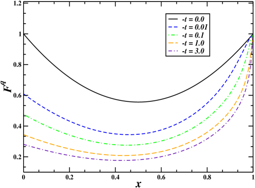
(b)

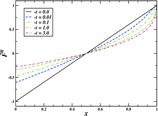
Figure 1: (Color online) (a) Plot of unpolarized GPD $F^{q}$ vs $x$ for fixed values of $-t$ in $GeV^{2}$ and (b) polarized GPD $\tilde{F^{q}}$ vs $x$ for fixed values of $-t$ in $GeV^{2}$, $\Lambda=20\mathrm{GeV}$. In both plots the normalization factor is chosen to compare with pire when $t=0$.

For the antiquark contributions we have similar integrals

$$I^{\prime}_{1}=\int{d^{2}q^{\perp}\over H}=\pi Log\Big{[}{\Lambda^{2}\over\mu^{2}+m^{2}x(1+x)+m^{2}}\Big{]}=I^{\prime}_{2}$$

$$I^{\prime}_{3}=\int{d^{2}q^{\perp}\over HH^{\prime}}=\int_{0}^{1}d\alpha{\pi\over Q(x,\alpha,{(\Delta^{\perp})}^{2})}$$ (7)

where $H={(q^{\perp})}^{2}+m^{2}x(1+x)+m^{2}$ and $H^{\prime}={(q^{\perp})}^{2}+{(\Delta^{\perp})}^{2}(1+x)^{2}+2q^{\perp}\cdot\Delta^{\perp}(1+x)+m^{2}x(1+x)+m^{2}$, and $Q(x,\alpha,{(\Delta^{\perp})}^{2})=m^{2}x(1+x)+m^{2}+\alpha(1-\alpha)(1+x)^{2}{(\Delta^{\perp})}^{2}$.

(a)
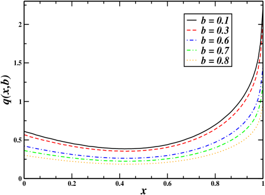
(b)

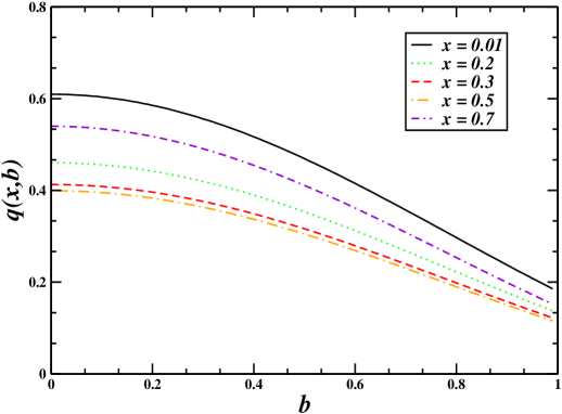
Figure 2: (Color online) (a)Plot of impact parameter dependent pdf $q(x,b)$ vs $x$ for fixed $b$ values and (b) $q(x,b)$ vs $b$ for fixed values of $x$ where we have taken $\Lambda$ = 20 $\mathrm{GeV}$ and $\Delta_{max}$= 3 GeV where $\Delta_{max}$ is the upper limit in the $\Delta$ integration. $b$ is in ${\mathrm{GeV}}^{-1}$ and $q(x,b)$ is in ${\mathrm{GeV}}^{2}$ .

For polarized photon the GPD $\tilde{F}^{q}$ can be calculated from the terms of the form $\epsilon^{2}_{\lambda}\epsilon^{1*}_{\lambda}-\epsilon^{1}_{\lambda}\epsilon^{2*}_{\lambda}$ pire . We consider the terms where the photon helicity is not flipped. This can be written as,

$$\tilde{F}^{q} = \sum_{q}{\alpha e_{q}^{2}\over 4{\pi}^{2}}\Big{[}(x^{2}-(1-x)^{2})(I_{1}+I_{2}+LI_{3})+2m^{2}I_{3}\big{]}\theta(x)\theta(1-x)$$ (8)

$$+\sum_{q}{\alpha e_{q}^{2}\over 4{\pi}^{2}}\Big{[}(x^{2}-(1+x)^{2})(I^{\prime}_{1}+I^{\prime}_{2}+L^{\prime}I^{\prime}_{3})+2m^{2}I^{\prime}_{3}\Big{]}\theta(-x)\theta(1+x)$$

(a)

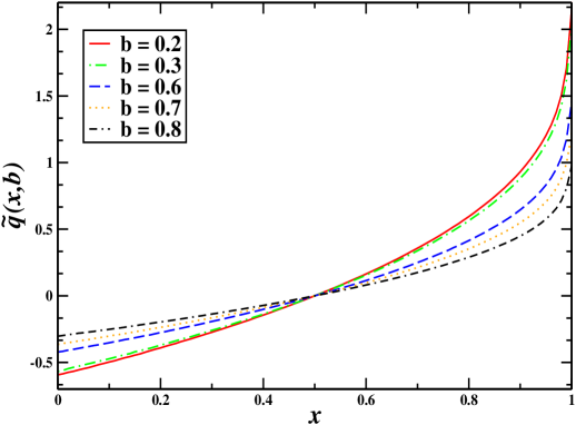
(b)

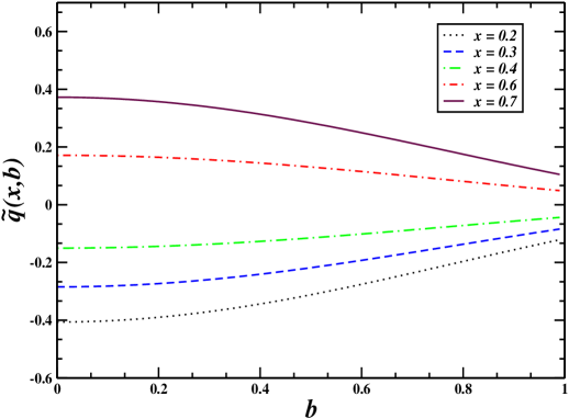
Figure 3: (Color online) (a)Plot of impact parameter dependent pdfs $\tilde{q}(x,b)$ vs $x$ for fixed $b$ values and (b) $\tilde{q}(x,b)$ vs $b$ for fixed values of $x$ where we have taken $\Lambda$ = 20 $\mathrm{GeV}$ and $\Delta_{max}$= 3 GeV where $\Delta_{max}$ is the upper limit in the $\Delta$ integration. $b$ is in ${\mathrm{GeV}}^{-1}$ and $\tilde{q}(x,b)$ is in ${\mathrm{GeV}}^{2}$.

In analogy with the impact parameter dependent parton distribution of the proton, we introduce the same for the photon. By taking a Fourier transform with respect to the transverse momentum transfer $\Delta^{\perp}$ we get the GPDs in the transverse impact parameter space.

$$q(x,b^{\perp}) = {1\over(2\pi)^{2}}\int d^{2}\Delta^{\perp}e^{-i\Delta^{\perp}\cdot b^{\perp}}F^{q}$$ (9)

$$= {1\over 2\pi}\int\Delta d\Delta J_{0}(\Delta b)F^{q};$$

$$\tilde{q}(x,b^{\perp}) = {1\over(2\pi)^{2}}\int d^{2}\Delta^{\perp}e^{-i\Delta^{\perp}\cdot b^{\perp}}\tilde{F}^{q}$$ (10)

$$= {1\over 2\pi}\int\Delta d\Delta J_{0}(\Delta b)\tilde{F}^{q};$$

where $J_{0}(z)$ is the Bessel function; $\Delta=|\Delta^{\perp}|$ and $b=|b^{\perp}|$. In the numerical calculation, we have introduced a maximum limit $\Delta_{max}$ of the $\Delta$ integration which we restrict to satisfy the kinematics $-t<<Q^{2}$ hadron_optics ; chiral ; quark ; model . $q(x,b^{\perp})$ gives the distribution of partons in this case inside the photon in the transverse plane. Like the proton, this interpretation holds in the infinite momentum frame and there is no relativistic correction to this identification because in light-front formalism, as well as in the infinite momentum frame, the transverse boosts act like non-relativistic Galilean boosts. $q(x,b^{\perp})$ gives simultaneous information about the longitudinal momentum fraction $x$ and the transverse distance $b$ of the parton from the center of the photon and thus gives a new insight to the internal structure of the photon. The impact parameter distribution for a polarized photon is given by $\tilde{q}(x,b^{\perp})$.

(a)

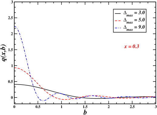
(b)

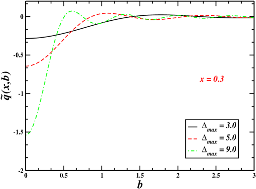
Figure 4: (Color online) Plots of impact parameter dependent pdfs (a) ${q}(x,b)$ and (b) $\tilde{q}(x,b)$ vs $b$ for a fixed $x$; where we have taken $\Lambda$ = 20 $\mathrm{GeV}$ for different values of $\Delta_{max}$ in GeV. $b$ is in ${\mathrm{GeV}}^{-1}$ and $q(x,b)$ as well as $\tilde{q}(x,b)$ are in ${\mathrm{GeV}}^{2}$.

Numerical results

We have plotted the unpolarized GPD $F^{q}$ and the polarized GPD $\tilde{F}^{q}$ for the photon in Figs 1(a) and (b) respectively as functions of $x$ and for different values of $t=-{(\Delta^{\perp})}^{2}$. In all plots we took the momentum transfer to be purely in the transverse direction. We took $m=3.3$ MeV; $\Lambda=Q=20\mathrm{GeV}$, $\mu=0$ MeV and $\Delta_{max}$= 3.0 GeV where $\Delta_{max}$ is the upper limit of the $\Delta^{\perp}$ integration in the Fourier transform. It is to be noted that the photon structure function $F_{2}^{\gamma}(x,Q^{2})$ has been explored over a wide kinematical range, namely $0.001<x<0.9$ and $1.9<Q^{2}<780\mathrm{GeV}^{2}$ buras . However, here we restrict ourselves to study the general features of the photon GPDs at a fixed scale rather than the scale evolution. We have divided the GPDs by the normalization constant to compare with pire in the limit of zero $t$. Indeed they agree. As $-t$ increases, $F^{q}$ becomes more and more asymmetric with respect to $x=1/2$ : this asymmetry is prominent for lower values of $x$ which is expected as the $\Delta^{\perp}$ or $t$ dependence is associated with a $(1-x)^{2}$ factor (see the analytic expressions). The slope of the polarized GPD changes with increasing ${(\Delta^{\perp})}^{2}$. Note that in pire as well as in the solid line in figs 1(a) and 1(b), the subleading mass terms are not taken into account. It is to be noted that in all plots we have taken $0<x<1$ for which the contribution comes from the active quark in the photon ($q{\bar{q}}$). As $x\rightarrow 1$, most of the momentum is carried by the quark in the photon and the GPDs become independent of $t$. The Fourier transform (FT) of the unpolarized GPD $F^{q}$ is plotted in Fig. 2. Fig. 2 (a) shows the plot of the impact parameter dependent pdf of the photon as a function of $x$ and for fixed impact parameter $b=\mid b^{\perp}\mid$. Fig. 2 (b) shows the same but as a function of $b$ and for fixed $x$. The smearing in $b^{\perp}$ space reveals the partonic substructure of the photon and its ’shape’ in transverse space. In the ideal definition the Fourier transform over $\Delta$ should be from $0$ to $\infty$. In this case the $\Delta^{\perp}$ independent terms in $F^{q}$ and $\tilde{F}^{q}$ would give $\delta^{2}(b^{\perp})$ in the impact parameter space. This means in the case of no transverse momentum transfer, the photon behaves like a point particle in transverse position space. The distribution in transverse space is a unique feature accessible only when there is non-zero momentum transfer in the transverse direction. From the plots it can be seen that for fixed $b$, $q(x,b)$ decreases slowly with $x$ till $x\approx 1/2$ then increases. The behavior in impact parameter space is qualitatively different than a dressed quark target and also from phenomenological models of proton GPDs. For a dressed quark target the leading contribution to the GPD comes from the single particle sector of the Fock space expansion, which in impact parameter space gives a delta function peak. This contributes at $x=1$. For large values of $x$ the peak in impact parameter space becomes sharper and narrower, that means there is a higher probability of finding the active quark near the transverse center of momentum quark . In the phenomenological parametrization of proton GPDs where a spectator model with Regge-type modification was used, the GPDs have a different behavior in impact parameter space, the $u$ quark GPDs increase with increasing $x$ for fixed $b$, reaches a maximum, then decrease. The peak decreases with increasing $b$ model . In the case of a photon there is no single particle contribution, and the distribution in $b$ space purely reveals the internal $q{\bar{q}}$ structure of the photon. Here near $x\approx 1/2$ the peak in $b$ space is very broad which means that the parton distribution is more dispersed when the $q$ and ${\bar{q}}$ share almost equal momenta. The parton distribution is sharper both for smaller $x$ and larger $x$. In Figs 3 (a) and (b) we have plotted the polarized distribution in impact parameter space. Fig. 3 (a) shows it as a function of $x$ for fixed $b$ values and fig 3 (b) shows it as a function of $b$ for fixed $x$ values. The slope decreases for higher $b$. The sign of the GPD changes at $x=1/2$, at which point the GPD and the pdf in impact parameter space becomes zero. The distributions are approximately symmetric about $x=1/2$ in impact parameter space; as $x\rightarrow 1$ the distribution increases sharply as the GPDs become independent of $t$; this is similar to $q(x,b)$. For fixed $x$, $\tilde{q}(x,b)$ as a function of $b$ becomes broader as $x$ increases until $x=1/2$. For larger values of $x$, it changes sign. In the plots we have taken the upper limit of the Fourier transform to be much smaller than $\Lambda$. The dependence of $q(x,b)$ and $\tilde{q}(x,b)$ on $\Delta_{max}$ is shown in Figs. 4 (a) and (b) respectively. As $\Delta_{max}$ increases, the distribution becomes sharper in impact parameter space. This shows that larger momentum transfer probes the partons near the transverse center of the photon.

Conclusion

We presented a first calculation of the generalized parton distributions of the photon, both polarized and unpolarized, when the momentum transfer in the transverse direction is non-zero; at zeroth order in $\alpha_{s}$ and leading order in $\alpha$; we calculated at leading logarithmic order and also kept the mass terms at the vertex. We took the skewness to be zero. We express the GPDs in terms of overlaps of the photon light-front wave functions. We considered the matrix elements when the photon helicity is not flipped. When the momentum transfer in the transverse direction is non-zero, one also has helcity flip contributions, which will be treated in a later work. In our case only the diagonal parton number conserving overlaps contribute. We considered both the quark and the antiquark contributions. The GPDs thus probe the two particle $q{\bar{q}}$ structure of the photon. Taking a Fourier transform (FT) with respect to $\Delta_{\perp}$ we obtain impact parameter dependent parton distribution of the photon. We plot them for both polarized and unpolarized photon. The parton distributions in impact parameter space show distinctive features compared to the proton and also compared to a dressed quark, which can be taken as an example of a spin $1/2$ composite relativistic system consisting of a quark and a gluon. It is to be noted that a complete understanding of the photon GPDs beyond leading logs would require also the non-pointlike hadronic contributions which will be model dependent pire . However, the GPDs of the photon calculated here may act as interesting tools to understand the partonic substructure of the photon. Accessing them in experiment is a challenge. On the theoretical side, the next step would be to investigate the photon GPDs when there is non-zero momentum transfer both in the transverse and in the longitudinal direction as well as a perturbative study of the general properties of GPDs like positivity and polynomiality conditions and sum rules.

Acknowledgments

This work is supported by BRNS grant Sanction No. 2007/37/60/BRNS/2913 dated 31.3.08, Govt. of India. We thank B. Pire for suggesting this topic and B. Pire, S. Wallon and M. Diehl for helpful discussions. AM thanks Ecole Polytechnique for support where part of this work was done.

References

- (1) T. F. Walsh and P. M. Zerwas, Phys. Lett. B 44, 95 (1974).
- (2) E. Witten, Nucl. Phys. B 120, 189 (1977).
- (3) A. Buras, Acta. Phys. Polon. B 37, 683 (2006).
- (4) S. Friot, B. Pire, L. Szymanowski, Phys. Lett. B 645 153 (2007).
- (5) M. El Beiyad, B. Pire, L. Szymanowski, S. Wallon, Phys. Rev. D 78, 034009 (2008).
- (6) For reviews on generalized parton distributions, and DVCS, see M. Diehl, Phys. Rept, 388, 41 (2003); A. V. Belitsky and A. V. Radyushkin, Phys. Rept. 418 1, (2005); K. Goeke, M. V. Polyakov, M. Vanderhaeghen, Prog. Part. Nucl. Phys. 47, 401 (2001); S. Boffi, B. Pasquini, Riv.Nuovo Cim.30:387,2007.
- (7) M. Burkardt, Int. J. Mod. Phys. A 18, 173 (2003); M. Burkardt, Phys. Rev. D 62, 071503 (2000), Erratum- ibid, D 66, 119903 (2002); J. P. Ralston and B. Pire, Phys. Rev. D 66, 111501 (2002).
- (8) D. Chakrabarti, R. Manohar, A. Mukherjee, Phys.Rev. D79, 034006,(2009).
- (9) S. J. Brodsky, D. Chakrabarti, A. Harindranath, A. Mukherjee and J. P. Vary, Phys. Lett. B 641, 440 (2006); Phys. Rev. D 75, 014003 (2007).
- (10) S. J. Brodsky, M. Diehl, D. S. Hwang, Nucl. Phys. B 596, 99 (2001); M. Diehl, T. Feldman, R. Jakob, P. Kroll, Eur. Phys. J. C 39, 1 (2005).
- (11) W. M. Zhang, A. Harindranath, Phys. Rev. D48, 4881 (1993).
- (12) A. Harindranath, R. Kundu, W. M. Zhang, Phys. Rev. D 59, 094013,(1999).
- (13) D. Chakrabarti and A. Mukherjee, Phys.Rev.D72, 034013 (2005); Phys. Rev. D71, 014038 (2005).
- (14) D. Chakrabarti, R. Manohar, A. Mukherjee, Phys. Lett. B 682, 428 (2010); R. Manohar, A. Mukherjee, D. Chakrabarti, Phys.Rev.D83, 014004,(2011).