Variational approximations to homoclinic snaking in continuous and discrete systems

Abstract

Localised structures appear in a wide variety of systems, arising from a pinning mechanism due to the presence of a small-scale pattern or an imposed grid. When there is a separation of lengthscales, the width of the pinning region is exponentially small and beyond the reach of standard asymptotic methods. We show how this behaviour can be obtained using a variational method, for two systems. In the case of the quadratic-cubic Swift-Hohenberg equation, this gives results that are in agreement with recent work using exponential asymptotics. Secondly, the method is applied to a discrete system with cubic-quintic nonlinearity, giving results that agree well with numerical simulations.

I Introduction

This paper is concerned with the phenomenon of pinning of fronts in nonlinear dynamical systems. For systems that exhibit bistability of two uniform states, a front connecting these two states will normally drift in one direction, depending on which of the two states is preferred. At a particular parameter value, known as the Maxwell point, there is no preference between the two states and a stationary front exists. However, in systems where there is an underlying structure, on a scale that is typically small compared with the lengthscale of the front, a front can become locked to this structure. This mechanism allows a stationary front to exist over a range of parameter values around the Maxwell point, known as the pinning region. Placing two fronts back-to-back creates a localized state, and the bifurcation diagram plotting the length of this localized solution against the control parameter has a snaking structure, involving a sequence of saddle-node bifurcations in near-perfect alignment. Since the spatial structure of such a localized state departs from and then returns to, a uniform state, the phenomenon has become known as “homoclinic snaking”. See knob08 ; dawe10 for a review of the subject and some open questions.

There are two distinct scenarios in which homoclinic snaking appears. In the first of these, the underlying structure is provided by pattern formation. A physical system, for example convection in fluids bens88 ; nepo94 , a vibrated granular material, buckling of a solid cylinder hunt00 , optical systems firt07 or gas discharge experiments will90 ; will91 , has an instability leading to the formation of a regular periodic pattern as a parameter is varied. If this bifurcation is subcritical, there is bistability between the uniform and the patterned states. Near the onset of pattern formation, a subcritical Ginzburg-Landau equation can be derived bens88 ; budd05 ; burk07_2 , which has front-like solutions connecting the two states. However, this equation does not capture the locking mechanism. The localised states have been found numerically in many studies saka96 ; burk06 ; beck09 that use the Swift-Hohenberg equation as a simple model for pattern formation.

A second situation in which locked fronts appear is in discretized forms of partial differential equations, where there is a locking effect to the imposed lattice. Examples include stationary solutions of the discrete bistable nonlinear Schrödinger equation carr06 ; chon09 ; chon11 , which leads to a subcritical Allen-Cahn equation tayl10 , optical cavity solitons yuli08 ; yuli10 , and discrete systems with a weakly broken pitchfork bifurcation cler11 . This situation also arises whenever a bistable system is solved numerically on a spatial grid.

An interesting and challenging question is to determine the width in parameter space of the region in which stationary localized solutions exist. Numerical simulations indicate that this pinning region becomes very small as the separation of the two length-scales increases saka96 ; burk07_2 . In fact the region is exponentially small, or beyond all orders. This is related to the fact that a conventional multiple-scales asymptotic method cannot describe the locking effect, since it regards to the two lengthscales as independent, while in fact the locking mechanism involves an explicit interaction between the short and long lengthscale. The necessary exponential asymptotics calculations, involving truncating a divergent asymptotic series at an optimal point and obtaining an equation for the exponentially small remainder term, have recently been carried out for the Swift-Hohenberg equation with quadratic-cubic nonlinearities kozy06 ; chap09 and cubic-quintic nonlinearities dean11 . However, these calculations are extremely cumbersome and include an undetermined constant that must either be obtained numerically either by fitting to numerical results chap09 or by approximately solving a complicated recurrence relation dean11 .

In this paper we use variational methods to obtain scaling laws for the structure of the snaking region, building on the work in a previous short paper that studied the cubic-quintic Swift-Hohenberg equation susa11 . Of course, not all systems that exhibit homoclinic snaking have a variational structure, but most of those previously studied do. The variational method is dependent on good initial ansatz, but this is known in the cases studied here. For pattern forming problems near onset, it is known that the solution can be described by a slowly varying envelope function multiplied by a sinusoidal wave. Furthermore, the form of the envelope function is known from the standard asymptotic analysis, and can be obtained to higher order if required. Thus there is no guesswork involved in the method. Calculating the integrals in the Lagrangian automatically leads to exponentially small terms, and from these we can obtain the phase of the locked states that is inaccessible to the usual asymptotic expansion. Note that variational methods have been used before to study localized states on lattices carr06 ; chon11 , but not in the slowly-varying regime that is studied here. Also in the continuous case, variational methods have been used wade00 , but not in the snaking regime.

Here, we consider two equations, namely the quadratic-cubic Swift–Hohenberg equation and the discrete cubic-quintic Schrödinger equation, also known as the spatially discrete Allen–Cahn equation, representing continuous and discrete systems, respectively. The first equation is discussed in Section II. The results are then compared with numerical results obtained by continuation in Section II.3. The second equation is studied in Section III. The scaling calculated analytically using the variational method is then compared with computational results, where good agreement is obtained. Conclusions are in Section IV.

II The quadratic-cubic Swift-Hohenberg equation

The quadratic-cubic Swift-Hohenberg equation is given by

$$\partial_{t}u=ru-\left(1+\partial_{x}^{2}\right)^{2}u+b_{2}u^{2}-b_{3}u^{3}.$$ (1)

This equation represents a simple model for pattern forming systems that do not have a symmetry under sign reversal of the dependent variable $u$, and has been very widely used to illustrate homoclinic snaking beck09 ; budd05 ; burk06 ; kozy06 . The Lagrangian for (1) is

$$\mathcal{L}=\int_{-\infty}^{\infty}\left(\frac{u_{xx}^{2}}{2}-{u_{x}^{2}}+(1-r)\frac{u^{2}}{2}-\frac{b_{2}}{3}u^{3}+\frac{b_{3}}{4}u^{4}\right)dx.$$ (2)

It can easily be shown that $\mathcal{L}$ decreases with time, so stable stationary states of (1) correspond to minima of (2). It will be assumed that $b_{3}>0$; in this case $u$ can be rescaled to set $b_{3}=1$. In (1), the bifurcation at $r=0$ is subcritical (allowing localised patterns) if $b_{2}>\sqrt{27b_{3}/38}$.

Figure 1 shows the bifurcation diagram for (1) obtained by a numerical continuation method for $b_{2}=1.5$, $b_{3}=1$, with periodic boundary conditions in a domain of length $l=82\pi$. The norm $N$ plotted is defined by

$$N^{2}=\int_{-l/2}^{l/2}u^{2}\,dx.$$ (3)

The periodic solution (dashed line) bifurcates subcritically and becomes stable at a saddle-node bifurcation at $r\approx-0.186$. Two branches of localized solutions bifurcate from the periodic state at a very small value of $r$ and form an intertwined snaking pattern near the Maxwell point at $r\approx-0.151$. On one of these branches, the maximum of the envelope function coincides with a minimum of the periodic pattern, and on the other it coincides with a maximum, so the two states have a phase difference of $\pi$. Solutions along the former branch are shown in Figure 2. The first figure, for $r=-0.01$, shows a slow spatial modulation that can be represented by an envelope in the form of a sech function (see Sec. II.1). For $r=-0.05$ the amplitude modulation occurs over a shorter lengthscale but can still be represented by the sech function. The third graph shows $u(x)$ at the first saddle-node bifurcation, $r=-0.146$, and the final graph is at a saddle-node bifurcation higher up the graph where $r=-0.158$ and $N=5.15$. At this stage the solution resembles two fronts connecting the periodic solution to the state $u=0$ (see Sec. II.2).

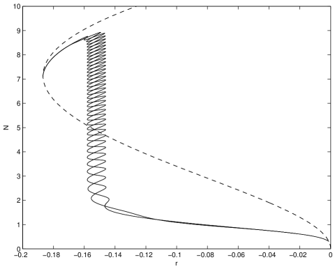
Figure 1: Bifurcation diagram of (1) for $b_{2}=1.5$, $b_{3}=1$. The dashed line is the periodic solution. The two solid lines are the localized snaking solutions.

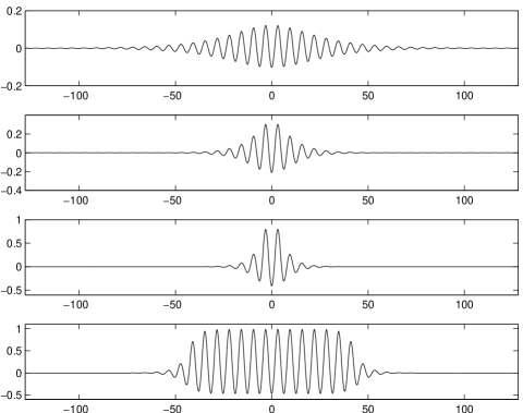
Figure 2: Localized solutions on one branch of Fig. 1. From top to bottom, $r=-0.01$, $r=-0.05$, $r=-0.146$, $r=-0.158$ ($N=5.15$).

II.1 Analysis of solutions near $r=0$

The analysis near $r=0$ can be performed in a similar way to that in susa11 . Motivated by the results from multiple scale expansions yang97 ; wade00 ; burk06 , we take the ansatz

$$u=A\operatorname{sech}(Bx)\cos(kx+\varphi)+C\operatorname{sech}^{2}(Bx),$$ (4)

from which we obtain that the norm (3) is given by

$$N^{2} = \frac{1}{3B}\left(3A^{2}+4C^{2}\right)+\frac{3A\pi}{B^{3}}\left(C(B^{2}+k^{2})\cos(\varphi)\operatorname{sech}\left(\frac{k\pi}{2B}\right)+ABk\cos(2\varphi)\operatorname{csch}\left(\frac{k\pi}{B}\right)\right).$$ (5)

Substituting the ansatz (4) into the Lagrangian (2) yields the effective Lagrangian

$$L_{eff} = \frac{2C^{2}}{315B}\left(36b_{3}C^{2}-56b_{2}C-168B^{2}+240B^{4}+105-105r\right)$$ (6)

$$-\frac{A^{2}}{30B}\left(-24b_{3}C^{2}+20b_{2}C-7B^{4}-30k^{2}B^{2}+10B^{2}-15k^{4}+30k^{2}+15(r-1)\right)+\frac{b_{3}}{8B}A^{4}$$

$$+{\frac{\pi Ak^{2}}{720B^{7}}}\left(-60b_{2}C^{2}k^{2}B^{2}+45\,A^{2}b_{3}\,C\,B^{2}k^{2}+B^{4}\left(240Ck^{4}-180A^{2}b_{2}+720C(1-k^{2})\right)+2b_{3}C^{3}k^{4}\right)$$

$$\times\cos(\varphi)\left(e^{-\frac{k\pi}{2B}}+\mathcal{O}\left(e^{-\frac{k\pi}{B}}\right)\right).$$

It is immediately clear from (6) that the phase $\varphi$ is determined by exponentially small terms, since the parameter $B$ is expected to be small, with $1/B$ representing the lengthscale of the modulation of the pattern. Furthermore, (6) shows that steady states (extrema of $L_{eff}$) exist if $\varphi$ is a multiple of $\pi$ yang97 . There are two distinct states, $\varphi=0$ and $\varphi=\pi$, both corresponding to even solutions but with the maximum of the envelope function $\operatorname{sech}(Bx)$ coinciding with a maximum or minimum of the wave $\cos(kx)$, as shown by the numerical continuation method in the previous section. Note that this result does not depend on our choice of ansatz. For any slowly varying, even modulation function $f(Bx)$, the integrals in the Lagrangian involve powers of $f(Bx)$ and its derivatives multiplied by $\cos(kx)\cos(\varphi)$, yielding an exponentially small quantity multiplied by $\cos(\varphi)$, and hence stationary states with $\varphi=0,\pi$. In the symmetric cubic-quintic case susa11 , only even powers appear in the integrals, leading to integrals only involving $\cos(2kx)\cos(2\varphi)$, and hence stationary solutions with $\varphi=0,\pi/2,\pi,3\pi/2$.

Applying the Euler-Lagrange formulation to the effective Lagrangian

$$\frac{\partial}{\partial\alpha}\mathcal{L}_{eff}=0,$$ (7)

gives us a system of nonlinear equations for $\alpha$, with $\alpha=A,\,B,\,C,\,k,\,\varphi$, that make (4) an approximate solution of (1).

Neglecting the exponentially small terms in the effective Lagrangian (6), the Euler-Lagrange equations can be solved perturbatively about $r=0$ to yield

$$A = \sqrt{\frac{8}{4b_{2}^{2}-3b_{3}}}\sqrt{-r}+\mathcal{O}((-r)^{3/2}),$$ (8)

$$B = \frac{1}{2}\sqrt{-r}+\mathcal{O}(-r),$$ (9)

$$C = -\frac{4b_{2}}{4b_{2}^{2}-3b_{3}}r+\mathcal{O}((-r)^{3/2}),$$ (10)

$$k = \sqrt{1-B^{2}}=1+\frac{r}{8}.$$ (11)

It is important to note that the presence of $C\neq 0$ plays an important role in the calculations above, unlike the case of the cubic-quintic equation susa11 where it was possible to include only the first term in (4). Taking $C=0$ would result in the leading order expression of $A$ independent of $b_{2}$, which is incorrect. This occurs because when $C=0$ the cubic term in the Lagrangian, which corresponds to the crucial symmetry-breaking quadratic term in (1), does not contribute to the Lagrangian integral except through an exponentially small term. Note that $C=b_{2}A^{2}/2$, a result that is also easily be obtained at second order in the asymptotic analysis of the problem. A similar Lagrangian method was used by Wadee and Bassom wade00 , using more terms in the ansatz (4) but with $\varphi=0$. The results above for $A$ and $C$ are almost the same as those obtained using multiple scale expansions wade00 ; burk06 . A slight difference arises as we have for simplicity omitted a second-order term in $\operatorname{sech}^{2}(Bx)\cos(2kx+2\varphi)$; including this term would give exact agreement between the Lagrangian method and the asymptotic analysis. According to (8) the transition from a sub- to supercritical bifurcation occurs at $b_{2}^{2}/b_{3}=3/4$, which is very close to the true value of 27/38 kozy06 .

The equation (11) indicates a slight decrease in the wavenumber, corresponding to a slight increase in the wavelength of the patterns. As noted by Wadee and Bassom wade00 , this is simply a consequence of the linear dispersion relation; (11) can be obtained directly from the linear terms in (1) when $r<0$. Hence it is not surprising that the same wavenumber correction was found in the cubic-quintic case susa11 .

When neglecting the exponentially small terms, the phase-shift $\varphi$ at this order is arbitrary, which also agrees with the multiple scales result. However, taking into account the equation $\partial_{\varphi}\mathcal{L}_{eff}=0$, in which all the terms are exponentially small, $\varphi$ has to be a multiple of $\pi$, as mentioned above.

The ansatz (4) is only appropriate for small values of $|r|$, away from the Maxwell point (see Figs. 1 and 2). In the snaking region near the Maxwell point, the envelope of the localized states resembles two connected fronts. The following section introduces a suitable ansatz for this regime.

II.2 Analysis of solutions near the Maxwell point

For values of $b_{2}$ in the neighbourhood of

$$b_{20}=\sqrt{\frac{27}{38}b_{3}},$$ (12)

the bifurcation is only slightly subcritical and the Maxwell point is within reach of weakly nonlinear analysis. In this case the quadratic-cubic Swift-Hohenberg equation (1) has a front solution, which is approximately given by kozy06

$$u=A_{M}\frac{\cos{\left(x-\frac{1}{2\sqrt{734}}\ln\left(1+e^{a_{M}x}\right)\right)}}{\sqrt{1+e^{-a_{M}x}}},$$ (13)

with

$$A_{M} = \sqrt{\frac{38\sqrt{-r_{M}}}{\sqrt{734}b_{3}}},\quad a_{M}=\sqrt{-r_{M}},$$ (14)

$$r_{M} = -\frac{6859}{17616b_{3}}(b_{2}-b_{20})^{2}.$$ (15)

In analytically estimating the width of the snaking region in the equation using variational approximations, we will employ a front solution similar to (13). Considering this solution, one can note that the oscillation wave number $k$ of the front changes in space. In the limits $x\to\pm\infty$, $k\to 1$ and $(1-a_{M}(2\sqrt{734})^{-1})\approx 1$. Therefore, we will fix $k=1$ to simplify the analysis.

It turns out that as in the case of the $\operatorname{sech}$ solutions considered in the previous section, if only the leading order front solution (13) is used as the ansatz, the leading terms in the Lagrangian do not depend on $b_{2}$, giving qualitatively incorrect results. We therefore adopt an ansatz of the form

$$u=\frac{A\cos(x+\phi)}{\sqrt{1+e^{B(|x|-L)}}}+\frac{b_{2}A^{2}}{2(1+e^{B(|x|-L)})}.$$ (16)

The second term here arises at second order in the weakly nonlinear expansion wade00 , included for a similar reason as discussed in the previous section. This term is responsible for the upward displacement of the periodic pattern that is apparent in Fig. 2. To simplify the calculation we have set the value of the coefficient of this term in advance rather than leaving it as a free parameter. The asymptotic analysis includes another second-order term, proportional to $\cos 2(x+\varphi)$ wade00 , which is omitted partly in the interests of simplicity and partly because it is smaller by a factor of 9 than the term we have included.

Evaluation of the Lagrangian integral is considerably more complicated than in the cubic-quintic case susa11 . This is partly because of the two-term ansatz and partly because the dominant terms come from odd powers of the square root function, requiring integrals that cannot simply be computed using residues. These integrals can be evaluated in terms of multiplications of gamma functions of a complex argument, which in turn can be expanded using Stirling’s formula when $B$ is small, giving the anticipated exponentially small terms. There are a large number of these exponentially small terms, and the calculation is complicated by the fact that terms involving higher powers of $u$, which one might expect to give a smaller contribution, in fact all give exponentially small terms of the same order.

To illustrate some of the steps in the calculation, consider the term $\int_{-\infty}^{\infty}u^{2}dx$, which is the defined norm (3) and one of the terms in the Lagrangian density (2). Using the ansatz, this can be written as

$$\int_{-\infty}^{\infty}u^{2}dx=\int_{0}^{\infty}\frac{A^{2}\left(1+b_{2}^{2}A^{2}/2+e^{B(x-L)}\right)}{\left(1+e^{B(x-L)}\right)^{2}}$$

$$+\frac{2b_{2}A^{3}\cos(\phi)\cos(x)}{\left(1+e^{B(x-L)}\right)^{3/2}}+\frac{A^{2}\cos(2\phi)\cos(2x)}{1+e^{B(-L+x)}}\,dx,$$ (17)

after using the double-angle formula and the fact that the envelope function is even. The first term, that is independent of $\phi$, in the integral can be evaluated directly and gives the answer $A^{2}L\left(1+A^{2}b_{2}^{2}/2\right)-A^{4}b_{2}^{2}/(2B)+\mathcal{O}(e^{-BL})$. The integral of the third term can be found by using contour integration, similarly to that used in susa11 . Yet, we are not interested in the explicit expression of it, as it contributes to higher harmonic corrections in $\phi$. The second term is of our interest, giving a leading exponentially small contribution of order $\mathcal{O}(e^{-\frac{\pi}{B}})$. Unfortunately, the integral cannot be immediately evaluated by using the residue method as mentioned above. By using Mathematica, one will obtain that

$$\int_{0}^{\infty}\frac{\cos(x)\,dx}{\left(1+e^{B(x-L)}\right)^{3/2}}=\frac{ie^{-iL}\Gamma\left(\frac{3B+2i}{2B}\right)\Gamma\left(\frac{-i+B}{B}\right)}{\sqrt{\pi}}-\frac{ie^{iL}\Gamma\left(\frac{3B-2i}{2B}\right)\Gamma\left(\frac{i+B}{B}\right)}{\sqrt{\pi}}$$

$$+\frac{e^{BL}}{B}{\left[\frac{2e^{BL}\sqrt{1+e^{-BL}}}{1+e^{BL}}-{}_{2}F_{1}\left(\frac{i-B}{B},\frac{1}{2},\frac{i}{B},-e^{-BL}\right)-{}_{2}F_{1}\left(-\frac{i+B}{B},\frac{1}{2},-\frac{i}{B},-e^{-BL}\right)\right]},$$ (18)

where $\Gamma$ and ${}_{2}F_{1}$ are respectively the Gamma and the hypergeometric function.

The hypergeometric function can be written in a series form as

$${}_{2}F_{1}(a,b,c,z)=\sum_{n=0}^{\infty}\frac{(a)_{n}(b)_{n}}{(c)_{n}}\frac{z^{n}}{n!},$$

where $(\bullet)_{n}=\bullet(\bullet+1)\dots(\bullet+n-1)$ is the Pochhammer symbol. The series is convergent in our case, i.e. $0<B\ll 1$ and $BL\gg 1$, such that up to $\mathcal{O}(e^{-2BL})$

$${}_{2}F_{1}\left(\frac{i-B}{B},\frac{1}{2},\frac{i}{B},-e^{-BL}\right)=1-\frac{1}{2}e^{-BL}\left(1+iB\right),$$

$${}_{2}F_{1}\left(-\frac{i+B}{B},\frac{1}{2},\frac{-i}{B},-e^{-BL}\right)=1-\frac{1}{2}e^{-BL}\left(1-iB\right).$$

As for the Gamma function, it can be approximated by the Stirling’s formula

$$\Gamma(z)=\sqrt{\frac{2\pi}{z}}\left(\frac{z}{e}\right)^{z}\left(1+\mathcal{O}(\frac{1}{z})\right),$$

when $z$ is large enough in absolute value. Then, the first two terms on the right hand side of (18) can be approximated by

$$\frac{e^{-\frac{\pi}{B}}}{2B^{3/2}}\sqrt{\frac{\pi}{2}}\big{(}(-8+3B)\cos(L)+(8+3B)\sin(L)\big{)}.$$ (19)

Combining the approximations above, one will obtain that

$$\int_{-\infty}^{\infty}u^{2}dx=A^{2}L\left(1+\frac{1}{2}A^{2}b_{2}^{2}\right)-\frac{A^{4}b_{2}^{2}}{2B}$$

$$+\frac{A^{3}b_{2}}{B^{3/2}}\exp\left(-\frac{\pi}{B}\right)\sqrt{\frac{\pi}{2}}\cos(\phi)$$

$$\times\bigg{(}(-8+3B)\cos(L)+(8+3B)\sin(L)\bigg{)}.$$ (20)

The formula (20) indicates that in the snaking region, solutions with a larger norm correspond to longer plateaus.

Performing the same calculations to all the terms in the Lagrangian (2) yields the effective Lagrangian

$$\mathcal{L}_{eff} = \frac{A^{2}}{1920B}(15B^{4}+480B^{2}-160A^{2}b_{2}^{2}B^{2}+16A^{2}b_{2}^{2}B^{4}+480A^{2}b_{2}^{2}+480A^{2}rb_{2}^{2}$$ (21)

$$+240A^{4}b_{2}^{4}-360A^{2}b_{3}-1080A^{4}b_{3}b_{2}^{2}-110A^{6}b_{3}b_{2}^{4})$$

$$+\frac{LA^{2}}{96}(18A^{2}b_{3}-24A^{2}b_{2}^{2}-48r-24A^{2}rb_{2}^{2}-8A^{4}b_{2}^{4}+36A^{4}b_{3}b_{2}^{2}+3A^{6}b_{3}b_{2}^{4})$$

$$+\cos(\varphi){\frac{{A}^{3}\sqrt{2}\sqrt{\pi}b_{2}}{420}}{e^{{{-\pi}/{B}}}}{B}^{-7/2}\left(K_{+}\cos(L)+K_{-}\sin(L)\right)$$

$$+\mathcal{O}\left(e^{\frac{-2\pi}{B}}(\sin(2L),\cos(2L)),e^{-BL}\right),$$

where

$$K_{\pm} = \pm 56\,{A}^{4}b_{2}^{2}{b_{3}}+280\,{A}^{2}b_{2}^{2}B-420\,{A}^{2}{b_{3}}\,B$$ (22)

$$\pm 156\,{B}^{2}\pm 840\,r{B}^{2}-763\,{B}^{3}+70\,r{B}^{3}.$$

Consider first the terms that are not exponentially small, that is, the terms that do not involve the phase $\varphi$. Bearing in mind the anticipated scaling from (14), $A=\mathcal{O}(r^{1/4})$, the dominant terms in the bracket multiplied by $L$ are the first two terms, so $\mathcal{L}_{eff}$ only has a minimum over $L$ if at leading order, $b_{2}^{2}={3b_{3}/4}$. This is very close to the asymptotic result (12), and would be exactly the same if we had included the $\cos 2(x+\varphi)$ term mentioned above. We therefore set

$$b_{2}=\sqrt{3b_{3}/4}+\Delta,\quad|\Delta|\ll 1,$$ (23)

and expect that $\Delta$ and $B$ are $\mathcal{O}(r^{1/2})$, in which case the leading terms in the Lagrangian are

$$\mathcal{L}_{eff}^{lead} = \frac{A^{2}}{128B}(32B^{2}+32\sqrt{3b_{3}}A^{2}\Delta-45A^{4}b_{3}^{2})$$ (24)

$$+\frac{LA^{2}}{96}(45A^{4}b_{3}^{2}/2-48r-24\sqrt{3b_{3}}A^{2}\Delta).$$

Finding and solving the Euler-Lagrange equations by differentiating with respect to $L$, $A$ and $B$ gives the values

$$A^{2}=\frac{8\sqrt{3}\Delta}{15b_{3}^{3/2}},\quad B=\frac{\sqrt{10}\Delta}{5\sqrt{b_{3}}}$$ (25)

and yields the Maxwell point

$$r_{M}=-\frac{2\Delta^{2}}{5b_{3}}=-B^{2},$$ (26)

which is within $3\%$ of the asymptotic value given in (15). Note that the length $L$ is not determined by these equations. Substituting these values of $A$, $B$ and $r_{M}$ into the leading terms of the Lagrangian we find that the minimum is

$$Min(\mathcal{L}_{eff}^{lead})=\frac{4\sqrt{30}\Delta^{2}}{75b_{3}^{2}}.$$ (27)

Thus, although the Maxwell point can be determined by the condition that $\mathcal{L}$ is zero for both the zero state and the periodic state, the value of $\mathcal{L}$ is not zero for the localized state, due to the presence of the fronts. In fact, $\mathcal{L}$ is positive and of the same order as $r$.

Considering now the exponentially small term involving $\varphi$, it is clear from $\partial_{\varphi}\mathcal{L}_{eff}=0$ that there are two distinct branches of stationary snaking solutions, with $\varphi=0$ and $\varphi=\pi$, corresponding to the centre of the localised pattern being a local maximum or minimum respectively. However, another possible way to satisfy $\partial_{\varphi}\mathcal{L}_{eff}=0$ is that the coefficient multiplying the $\cos\varphi$ term vanishes, i.e.

$$K_{+}\cos(L)+K_{-}\sin(L)=0.$$ (28)

Substituting the above values of $A$ and $B$, and taking the leading terms in $K_{\pm}$, solutions of this type occur for values of $L$ given by

$$\tan L=K_{+}/K_{-},$$ (29)

where $K_{\pm}$ is given in (22), which to the leading order is

$$K_{\pm}={\frac{8\sqrt[4]{30}\sqrt{\pi}}{7875\,b_{3}}}\,{{\left(\pm 307\,\sqrt{3}-210\,\sqrt{10}\right)}{{}}}.$$ (30)

Hence, for small $B$ these states exist if $L=-0.110219...+m\pi$ for integer values of $m$. These solutions have been referred to as “bridges” wade02 or “ladders” burk07 and were identified in the exponential asymptotics of (1) by Yang and Akylas yang97 and Chapman and Kozyreff chap09 . The ladder states (not shown in Fig. 1) have no reflection symmetry and connect the two snaking branches, bifurcating from them near the saddle-node bifurcations.

To find the snaking range, we set $\sin(\varphi)=0$ and $r=r_{M}+\delta r$, and the Lagrangian simplifies to

$$\mathcal{L}_{eff} = \frac{4\sqrt{30}\Delta^{2}}{75b_{3}^{2}}-\frac{\delta rA^{2}L}{2}$$ (31)

$$+e^{-\frac{\pi}{B}}\left(K_{+}\cos(L)+K_{-}\sin(L)\right),$$

with $K_{\pm}$ given in (30). This can be minimised over $L$ to give the exponentially small value of $\delta r$ for stationary solutions,

$${\delta r}=\frac{2e^{-\frac{\pi}{B}}}{A^{2}}\left(K_{-}\cos(L)-K_{+}\sin(L)\right).$$ (32)

The maximum value of $\delta r$ (half the width of the snaking region) is then, using the leading-order approximations for $b_{2}$, $A$ and $B$ given above,

$$\delta r_{m}={\frac{2e^{-\pi/B}}{525{\Delta}}}\,{{\sqrt{241249\pi b_{3}}\sqrt[4]{120}}}.$$ (33)

Note that the dependence of the snaking width on the small parameter $\Delta$ is very similar to that for the small parameter $b_{3}$ in the cubic-quintic case susa11 . The dependence in (33) is the same as that obtained by Kozyreff and Chapman kozy06 using the methods of exponential asymptotics, although the comparison is not immediate since they regard $b_{2}$ as the control parameter rather than $r$. Note that the numerical coefficient was determined by fitting in kozy06 .

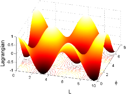
(a) (b)

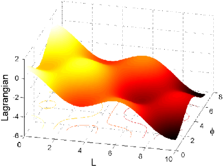
Figure 3: Surface plots of the simplified Lagrangian (34), (a) with $\delta r=0$ and (b) with $\delta r=0.4$.

A useful feature of the Lagrangian method is that we can examine the stability of steady states since we know that stable equilibria are local minima of the Lagrangian. Considering the exponentially small terms, with $A$ and $B$ fixed and $r=r_{M}+\delta r$, the dependence of $\mathcal{L}$ on $\delta r$, $L$ and $\varphi$ can be represented by the function

$$\mathcal{L}_{e}(\delta r,L,\varphi)=-\delta rL+\cos\varphi\cos(L-L_{0}),$$ (34)

where the phase shift $L_{0}$ satisfies (29) and for convenience we have set the constants to 1. Figure 3(a) shows a surface plot of $\mathcal{L}_{e}$ for $\delta r=0$. The solutions on the snaking branches, with $\varphi=0,\pi$, $L-L_{0}=m\pi$ are either maxima or minima, so are either stable or unstable with two positive eigenvalues. The ladder solutions at $\varphi=\pi/2,3\pi/2$, $L-L_{0}=\pi/2+m\pi$ are saddle points and are therefore always unstable. The surface plot for $\delta r=0.4$ is shown in Fig. 3(b). The symmetric snaking solutions remain at $\varphi=0,\pi$ but are shifted in $L$, while the ladder states are shifted in $\varphi$ but remain at the same values of $L$.

II.3 Numerical results

In this section we compare the above results from the variational method with numerical solutions of the quadratic-cubic Swift-Hohenberg equation (1). We have solved the equation numerically for localized states, using a pseudo-arclength continuation method with periodic boundary conditions, implemented with a Fourier spectral discretization. Plotted in the top left panel of Fig. 4 is the bifurcation diagram showing two branches of localized solutions for $b_{2}=1.3$ and $b_{3}=1$. In the same panel, shown in dashed lines are our analytical results obtained from (7) using the sech ansatz, where one can see that the variational calculation approximates the numerics very well for relatively small $|r|$. As $r$ decreases further and enters the snaking region, the approximation deviates from the numerics. In the top right panel, we plot the profile of a localized solution at $r=-0.06$ and its approximation.

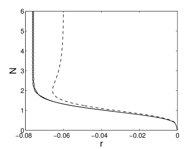
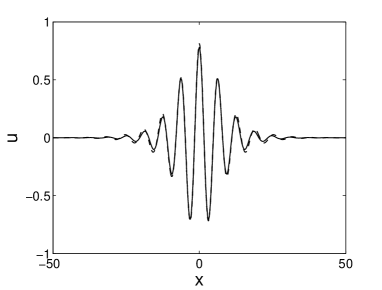
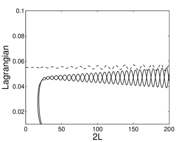
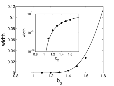
Figure 4: (a) The bifurcation diagram obtained numerically and our approximation obtained from solving (7) with the ansatz (4) for $b_{2}=1.3$. (b) A numerically obtained localized solution and its approximation from the variational formulation for $\varphi=0$ and $r=-0.06$. (c) The numerically computed Lagrangian (2) as a function of the length of the plateau $2L$, corresponding to panel (a). The dashed line is our approximation calculated from the effective Lagrangian (31). (d) The width of the snaking region as a function of $b_{2}$. Filled circles are numerical and solid lines are analytical, i.e. $2\delta r_{m}$ (33). The inset shows the same comparison in a log scale. In all the figures, $b_{3}=1$.

Considering Eqs. (8)–(11) one can conclude that for larger values of the parameter $b_{2}$, the parameter $|r|$ can be larger while keeping the amplitude $A$ (8) small. This implies that the sech ansatz can have a longer validity region for large $b_{2}$. It is important to note that the ansatz might be able to quantitatively capture the first snaking bifurcation for a larger value of $b_{2}$.

In panel (c) of the same figure, we plot the Lagrangian (2) corresponding to the bifurcation diagram (a) as a function of the length of the solution’s plateau $2L$, which is calculated numerically as

$$2L\approx\frac{8\int_{-l/2}^{l/2}u^{2}\,dx}{(u_{M}-u_{m})^{2}+2(u_{M}+u_{m})^{2}},$$

where $u_{M}=\max\{u\}$ and $u_{m}=\min{\{u\}}$. The integration is a definite integration over the computational domain. Plotted in the same panel is our effective Lagrangian (31). There is good agreement for the average numerical value of the Lagrangian and the qualitative nature of the oscillations, but the amplitude of the oscillations appears to be underestimated in the variational approximation. Note that the amplitude of the oscillations in $\mathcal{L}$ increases with $L$ since from (31) with $\delta r\propto\cos(L)$, there are oscillations of the form $L\cos(L)$.

Finally, in panel (d) we show the width of the snaking region as a function of $b_{2}$ numerically and analytically, where one can see that our approximation is in good agreement.

The numerical method can also be used to check the stability of the steady state solutions (since the Jacobian is already computed as part of the Newton-Raphson iteration). This confirms that the snaking states are in general either stable, or unstable with two small positive eigenvalues. One eigenvalue changes sign at the saddle-node bifurcation and another at the nearby bifurcation to the ladder states. The ladder states are found to be unstable with one positive eigenvalue, consistent with the fact that they are saddle points of the Lagrangian.

III Snaking in discrete systems

To illustrate the wide-ranging applicability of the variational method in describing the snaking behaviour, we analyse in this section an analogous problem in discrete systems. This turns out to be remarkably similar to the continuous case. Consider the system of ordinary differential equations

$$\frac{du_{n}}{dt}=C(u_{n+1}-2u_{n}+u_{n-1})+\mu u_{n}+2u_{n}^{3}-u_{n}^{5},$$ (35)

with the condition that $u_{n}\to 0$ as $n\to\pm\infty$. We assume that $C>0$ and look for stationary solutions of (35). This system has been considered in carr06 ; chon09 ; chon11 ; tayl10 , and very similar systems have been studied in yuli08 ; cler11 . The system (35) is interpreted as a discrete form of the nonlinear Schrödinger equation in carr06 ; chon09 , and a discrete subcritical Allen–Cahn equation in tayl10 . These previous studies have used numerical continuation to obtain bifurcation diagrams that show a very similar snaking structure to that seen in the continuous Swift-Hohenberg equation (1). Note however that (35) is not a discrete form of the Swift-Hohenberg equation. Rather it is a discrete form of the subcritical Ginzburg–Landau equation that describes the slowly varying envelope function for (1). Thus the snaking behaviour seen in (35) results from a locking mechanism to the discrete lattice, with the lattice points providing the analogue of the small-scale pattern in the Swift-Hohenberg equation. In view of this, computational investigation of the snaking in (35) is much easier than in (1), since there is no small-scale structure to resolve.

The grid-locking behaviour of fronts in (35) can be seen as an indication of numerical error in the finite-difference approximation of the bistable partial differential equation

$$\frac{\partial u}{\partial t}=\frac{\partial^{2}u}{\partial X^{2}}+\mu u+2u^{3}-u^{5}.$$ (36)

When (36) is discretized with second-order finite differences with mesh spacing $\epsilon$, the result is (35) with $C=\epsilon^{-2}$. Front-like solutions to (36) are travelling waves, for all values of $\mu$ except exactly at the Maxwell point. Thus the snaking branch of (35) indicates a range of values of $\mu$ where the numerical approximation incorrectly finds a stationary solution. It is therefore of interest to determine the width of this region for small values of $\epsilon$ (large values of $C$). An alternative scaling, similar to that in Sec. II, is to set $C=1$ and replace the 2 in (35) by a small parameter $b_{2}$; however we will use the form (35) to facilitate comparison with the previous work cited above.

The Lagrangian for (35) is

$$\mathcal{L}=\sum_{n=-\infty}^{\infty}\frac{C}{2}(u_{n+1}-u_{n})^{2}-\frac{\mu}{2}u_{n}^{2}-\frac{1}{2}u_{n}^{4}+\frac{1}{6}u_{n}^{6}.$$ (37)

Note that a variational method has been used in carr06 ; chon11 to study the case of small $C$, but here the focus will be on large $C$. The uniform solutions of (35) are given by $u_{n}=0$ and

$$u_{n}^{2}=1\pm\sqrt{1+\mu},$$ (38)

so there is a saddle-node bifurcation at $\mu=-1$ and there is bi-stability of both the zero state and the larger non-zero solution in (38) for $-1<\mu<0$. By finding the Lagrangian of this non-zero state it is straightforward to show that the Maxwell point is at $\mu=-3/4$ and so at this point the stable non-zero state is $u_{n}=\sqrt{3/2}$.

For large $C$ we expect the solution to (35) to be close to that of the continuous system (36). At the Maxwell point there is an exact stationary front-like solution of (36), $u(X)$, given by

$$u^{2}=\frac{A^{2}}{1+e^{\alpha X}},\mbox{ where }A^{2}=3/2,\ \alpha=\sqrt{3}.$$ (39)

In the discretized system, $u_{n}=u(\epsilon n)$, and we wish to consider a localized state linking two fronts. The ansatz analogous to that used in the continuous case (16) is then

$$u_{n}^{2}=\frac{A^{2}}{1+e^{\alpha\epsilon(|n-\phi|-L)}}.$$ (40)

Here, the length of the front (measured in terms of the number of mesh points) is $2L$ and $\phi$ is a phase variable, which is arbitrary at this stage but will be determined by exponentially small terms. If $\phi=0$ then $u_{j}=u_{-j}$ and the localized state is symmetrical and ‘site-centred’. Similarly, a ‘bond-centred’ symmetrical state, with the property $u_{j}=u_{1-j}$, can be obtained by setting $\phi=1/2$. Note that it is not necessary to include higher order terms in (40) as in (16); this is because (35) only has nonlinear terms with odd powers and therefore is more analogous to the cubic-quintic Swift-Hohenberg equation analysed with the Lagrangian approach in susa11 .

Consider now the sum $\sum_{n=-\infty}^{\infty}u_{n}^{2}$ that appears in $\mathcal{L}$. This can be evaluated by writing the sum as an integral of a function multiplied by a sum of $\delta$ functions, and then writing the sum of $\delta$ functions as a Fourier series:

$$\sum_{n=-\infty}^{\infty}u_{n}^{2} = \sum_{n=-\infty}^{\infty}\frac{A^{2}}{1+e^{\alpha\epsilon(|n-\phi|-L)}}$$

$$= \int_{-\infty}^{\infty}\frac{A^{2}}{1+e^{\alpha\epsilon(|x-\phi|-L)}}\sum_{n=-\infty}^{\infty}\delta(x-n)\,dx$$

$$= \int_{-\infty}^{\infty}\frac{A^{2}}{1+e^{\alpha\epsilon(|x-\phi|-L)}}\sum_{k=-\infty}^{\infty}e^{2ik\pi x}\,dx.$$

Note that $x$ here is not the same as $X$ in (36), rather it is a continuous form of the variable $n$. Of course the Fourier series representation of the $\delta$ function is not uniformly convergent, but the integral converges very rapidly – in fact exponentially. From the term $k=0$ we obtain an order one contribution

$$\int_{-\infty}^{\infty}\frac{A^{2}}{1+e^{\alpha\epsilon(|x-\phi|-L)}}\,dx=2LA^{2}+O(e^{-\alpha\epsilon L}).$$ (41)

The terms with $k=\pm 1$ give a contribution

$$\int_{-\infty}^{\infty}\frac{A^{2}(e^{2i\pi x}+e^{-2i\pi x})}{1+e^{\alpha\epsilon(|x-\phi|-L)}}\,dx$$ (42)

which is exponentially small in $\epsilon$, and the terms arising from larger values of $k$ are smaller by an exponentially small factor. Note that the integrals that are needed here, for the discrete case, are essentially exactly the same integrals that were needed for the continuous case in Sec. II and susa11 .

The integral (42) can be found using contour integration. For the term in $e^{2i\pi x}$ the contour is closed in the upper half plane and is dominated by the poles at $x=\phi\pm L+i\pi/(\alpha\epsilon)$. The sum of the residues at these two poles is

$$-2i\sin(2\pi L)e^{2i\pi\phi}\frac{A^{2}}{\alpha\epsilon}e^{\frac{-2\pi^{2}}{\alpha\epsilon}}.$$ (43)

The value of (42) is found by multiplying this by $2i\pi$ and adding the complex conjugate to account for the $e^{-2i\pi x}$ term. Hence the required sum is

$$\sum_{n=-\infty}^{\infty}u_{n}^{2}=2LA^{2}+8\pi\sin(2\pi L)\cos(2\pi\phi)\frac{A^{2}}{\alpha\epsilon}e^{\frac{-2\pi^{2}}{\alpha\epsilon}}+O(e^{\frac{-4\pi^{2}}{\alpha\epsilon}},e^{-\alpha\epsilon L}).$$ (44)

As in the continuous snaking case, we suppose that the exponential terms responsible for the grid locking dominate those from the interaction between the two fronts. This requires $L\gg\epsilon^{-2}$.

In a similar way it can be shown that

$$\sum_{n=-\infty}^{\infty}u_{n}^{4}=2LA^{4}-\frac{2A^{4}}{\alpha\epsilon}-\frac{8\pi A^{4}}{\alpha^{2}\epsilon^{2}}\cos(2\pi\phi)(2\pi\cos(2\pi L)-\alpha\epsilon\sin(2\pi L))e^{\frac{-2\pi^{2}}{\alpha\epsilon}}$$ (45)

and

$$\sum_{n=-\infty}^{\infty}u_{n}^{6}=2LA^{6}-\frac{3A^{6}}{\alpha\epsilon}-\frac{8\pi A^{6}}{\alpha^{3}\epsilon^{3}}\cos(2\pi\phi)(3\pi\alpha\epsilon\cos(2\pi L)+(2\pi^{2}-\alpha^{2}\epsilon^{2})\sin(2\pi L))e^{\frac{-2\pi^{2}}{\alpha\epsilon}},$$ (46)

where again terms of order $e^{\frac{-4\pi^{2}}{\alpha\epsilon}}$ and $e^{-\alpha\epsilon L}$ have been dropped. Note that for small $\epsilon$, the dominant exponentially small term comes from (46).

The remaining term required for the Lagrangian is

$$\sum_{n=-\infty}^{\infty}(u_{n+1}-u_{n})^{2}=\sum_{n=-\infty}^{\infty}A^{2}\left(\frac{1}{1+e^{\alpha\epsilon(|n+1-\phi|-L)}}-\frac{1}{1+e^{\alpha\epsilon(|n-\phi|-L)}}\right)^{2}.$$ (47)

As with the other terms, this can be written as an integral,

$$\int_{-\infty}^{\infty}A^{2}\left(\frac{1}{1+e^{\alpha\epsilon(|x+1-\phi|-L)}}-\frac{1}{1+e^{\alpha\epsilon(|x-\phi|-L)}}\right)^{2}(1+e^{2i\pi x}+e^{-2i\pi x}+\ldots)\,dx,$$

leading again to a part that is independent of $\phi$ and an exponentially small $\phi$-dependent term. For the part which does not depend on $\phi$, we can write the integrand as $(f(X+\epsilon)-f(X))^{2}$, where $f(X)=A/\sqrt{1+e^{\alpha X}}$, $X=\epsilon x$, and use Taylor expansion to find the dominant contribution to (47) in the form

$$\frac{1}{4}A^{2}\alpha\epsilon-\frac{1}{384}A^{2}\alpha^{3}\epsilon^{3}+O(\epsilon^{5}).$$

If the same method is applied for the exponentially small terms, it turns out that each term in the Taylor expansion yields a contribution that is of the same order after the exponentially small integral has been evaluated. Each term gives a contribution proportional to

$$\frac{A^{2}}{\alpha\epsilon}\cos(2\pi\phi)\sin(2\pi L)e^{\frac{-2\pi^{2}}{\alpha\epsilon}},$$

with a different numerical constant. Thus we know the scaling but not the magnitude of this term. Since (47) is multiplied by $C=\epsilon^{-2}$ in (37), this term is of the same order as the $u^{6}$ term in (37).

Using the above results, the leading terms in the Lagrangian (37) are

$$\mathcal{L}_{lead}=\frac{A^{2}\alpha}{8\epsilon}+\frac{A^{4}}{\alpha\epsilon}-\frac{A^{6}}{2\alpha\epsilon}+L\left(-\mu A^{2}-A^{4}+\frac{A^{6}}{3}\right).$$ (48)

By making this expression stationary with respect to $A$, $L$ and $\alpha$ we recover the results given earlier, $A^{2}=3/2$, $\alpha=\sqrt{3}$, $\mu=-3/4$.

To find the width of the snaking region, we set $\mu=-3/4+\Delta\mu$, and introduce the largest of the exponentially small terms, arising from the $u^{6}$ term and the difference term in (37), to obtain

$$\mathcal{L}=\frac{3\sqrt{3}}{8\epsilon}-\frac{3}{2}L\Delta\mu-\frac{(8\pi^{3}+D)A^{6}}{3\alpha^{3}\epsilon^{3}}\cos(2\pi\phi)\sin(2\pi L)e^{\frac{-2\pi^{2}}{\alpha\epsilon}},$$ (49)

where $D$ is an unknown constant representing the contribution from (47) where only the scaling is known.

By making (49) stationary with respect to $\phi$ it follows that snaking branches branches exist with $\phi=0$ or $\phi=1/2$, corresponding to the ‘site-centred’ and ‘bond-centred’ states found numerically. For these snaking branches, differentiating with respect to $L$ shows that

$$\Delta\mu\propto\frac{1}{\epsilon^{3}}\cos(2\pi L)e^{\frac{-2\pi^{2}}{\alpha\epsilon}}$$

so the scaling for the width of the snaking region in (35) for large $C$ is

$$\Delta\mu\propto{C^{3/2}}e^{-2\pi^{2}\sqrt{C/3}}.$$ (50)

Furthermore, differentiating (49) with respect to $\phi$ predicts that the ladder states, with $\sin(2\pi\phi)\neq 0$, occur for integer values of $L$.

To check the scaling predicted by (50), snaking curves for the equation were obtained numerically using a continuation software method. With 200 grid points it was possible to obtain snaking bifurcations up to a value $C=14$ (at which point the snaking width is of the order of $10^{-14}$). Figure 5 shows the numerically obtained snaking width multiplied by the predicted exponential factor $e^{2\pi^{2}\sqrt{C/3}}$. This shows a clear power-law behaviour, with a power very close to the value $3/2$ predicted by (50).

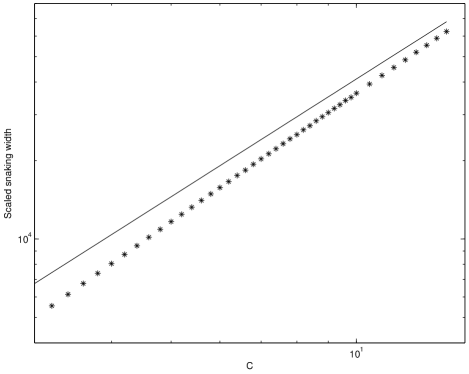
Figure 5: Log-log plot showing numerically obtained values of $\Delta\mu e^{2\pi^{2}\sqrt{C/3}}$ (points) together with the $3/2$ scaling law expected according to (50) (line).

IV Conclusion

In this paper we have used the variational approximation to study the snaking behaviour of localised patterns in the quadratic-cubic Swift–Hohenberg equation and the discrete bistable Allen–Cahn equation. With a simple ansatz, inspired by asymptotic analysis, the exponentially small terms responsible for the snaking appear in the Lagrangian. This enables the branches of snaking solutions to be found, along with the asymmetric ‘ladder’ states that link these branches.

These solutions cannot be found by a conventional multiple-scales method, since they involve a locking mechanism between the long and short scales, but are accessible through exponential asymptotics kozy06 ; chap09 . The Lagrangian approach provides a useful complement to the exponential asymptotics method. Both methods give the same scaling for the relationship between the width of the snaking region and the small parameter of the system.

We have shown that a close similarity exist between the pinning phenomena in continuous and discrete systems. This arises partly through the fact that the continuous limit of the discrete system considered is exactly the same as the Ginzburg–Landau equation describing spatial modulation of the pattern in the continuous case, and partly because the sums in the Lagrangian for the discrete case can be converted into integrals very similar to those that appear in the continuous problem.

The variational method has a number of advantageous features, in addition to the fact that the Lagrangian integral immediately generates the necessary exponentially small terms. Based on the minimisation of the Lagrangian, it is easy to distinguish between stable equilibria and unstable ones. Furthermore, although we have concentrated on the case of small parameters, for the purposes of comparison with asymptotic methods, the method is not restricted to this regime. In future work it may be possible to apply the method to cases where no parameters are small, and make useful comparisons with numerical or experimental results. An additional challenge will be to extend the results to two-dimensional systems chon09 ; beck09 ; mcca10 .

References

- (1) J.H.P. Dawes, Phil Trans. R. Soc. 368, 3519 (2010).
- (2) E. Knobloch, Nonlinearity 21, T45-T60 (2008).
- (3) D. Bensimon, B. I. Shraiman and V. Croquette, Phys. Rev. A 38, 5461 (1988).
- (4) A. A. Nepomnashchy, M. I. Tribelsky and M. G. Velarde, Phys. Rev. E 50, 1194 (1994).
- (5) G. W. Hunt et al. Nonlinear Dynamics 21, 3 (2000).
- (6) W.J. Firth, L. Columbo, and A.J. Scroggie, Phys. Rev. Letts. 99, 104503 (2007).
- (7) H. Willebrand, C. Radehaus, F.-J. Niedernostheide, R. Dohmen, H.-G. Purwins, Phys. Lett. A 149, 131 - 138 (1990).
- (8) H. Willebrand, F.-J. Niedernostheide, E. Ammelt, R. Dohmen, H.-G. Purwins, Phys. Lett. A 153, 437-445 (1991).
- (9) C. J. Budd and R. Kuske, Physica D 208, 73 (2005).
- (10) J. Burke and E. Knobloch, Chaos 17, 037102 (2007).
- (11) M. Beck, J. Knobloch, D.J.B. Lloyd, B. Sandstede and T. Wagenknecht, SIAM J. Math. Anal. 41(3) 936, (2009).
- (12) J. Burke and E. Knobloch, Phys. Rev. E 73, 056211 (2006).
- (13) H. Sakaguchi and H.R. Brand, Physica D 97, 274 (1996).
- (14) C. Chong and D.E. Pelinovsky, Discrete and Continuous Dynamical Systems Series S 4, 1019 (2011).
- (15) R. Carretero-Gonzalez, J.D. Talley, C. Chong and B.A. Malomed, Physica D, 216, 77-89 (2006).
- (16) C. Chong, R. Carretero-Gonzalez, B.A. Malomed and P.G. Kevrekidis, Physica D, 238, 126-136 (2009).
- (17) C. Taylor and J.H.P. Dawes, Phys. Lett. A 375, 14 (2010).
- (18) A.V. Yulin and A.R. Champneys, SIAM J. Appl. Dyn. Syst. 9, 391 (2010).
- (19) A.V. Yulin, A.R. Champneys and D.V. Skryabin, Phys. Rev. A 78, 011804 (2008).
- (20) M.G. Clerc, R.G. Elias and R.G. Rojas, Phil. Trans. Roy. Soc. A 369, 412 (2011).
- (21) S. J. Chapman and G. Kozyreff, Physica D 238, 319 (2009).
- (22) G. Kozyreff and S. J. Chapman, Phys. Rev. Lett. 97, 044502 (2006).
- (23) A.D. Dean, P.C. Matthews, S.M. Cox and J.R. King, preprint (2011).
- (24) H. Susanto and P.C. Matthews, Phys. Rev. E. 83, 035301(R) (2011).
- (25) M. K. Wadee and A. P. Bassom, J. Eng. Math. 38, 77 (2000).
- (26) T.-S. Yang and T. R. Akylas, J. Fluid Mech. 330, 215 (1997).
- (27) M. K. Wadee, C. D. Coman, and A. P. Bassom, Physica D 163, 26 (2002).
- (28) J. Burke and E. Knobloch, Phys. Lett. A 360, 681 (2007).
- (29) S. McCalla and B. Sandstede, Physica D 239, 1581 (2010).