Synchrotron radiation inside a dielectric cylinder

Abstract

We investigate the electromagnetic fields generated by a charged particle rotating inside a dielectric cylinder immersed into a homogeneous medium. The expressions for the bound modes of the radiation field are derived in both interior and exterior regions. The radiation intensity for the modes propagating inside the cylinder is evaluated by using two different ways: by evaluating the work done by the radiation field on the charge and by evaluating the energy flux through the cross-section of the cylinder. The relation between these two quantities is discussed. We investigate the relative contributions of the bound modes and the modes propagating at large distances from the cylinder to the total radiation intensity. Numerical examples are given for a dielectric cylinder in the vacuum. It is shown that the presence of the cylinder can lead to the considerable increase of the synchrotron radiation intensity.

PACS number(s): 41.60.Ap, 41.60.Bq

1 Introduction

Synchrotron radiation is an important tool in many disciplines. Its unique characteristics, such as high intensity and high collimation, have resulted in extensive applications (see, for example, [1, 2, 3]). Motivated by this, the investigation of mechanisms for the control of the radiation parameters is of great interest. Particularly important is the study of the influence of medium on the spectral and angular characteristics of the synchrotron radiation. The presence of medium can essentially change the characteristics of the high-energy electromagnetic processes. Moreover, new types of phenomena arise. Well-known examples are Cherenkov and transition radiations.

In [4]-[10] we have investigated the synchrotron radiation from a charge rotating around/inside a dielectric cylinder enclosed by a homogeneous medium. It has been shown that under the Cherenkov condition for the material of the cylinder and the particle velocity, strong narrow peaks appear in the angular distribution of the radiation intensity in the exterior medium. At these peaks the radiated energy exceeds the corresponding quantity in the case of a homogeneous medium by several orders of magnitude. Similar features for the radiation generated by a charge moving along a helical orbit have been discussed in [11]-[14]. The case for an electron rotating around/inside a dielectric ball has been considered in [15]-[18].

In the previous investigations of the radiation from a charge rotating around/inside a dielectric cylinder we have considered the radiation intensity in the exterior region at large distances from the cylinder. In addition to this part there is radiation which propagates inside the cylinder and it is of interest to investigate the relative contribution of these modes to the total intensity. In the present paper we consider the radiation intensity inside a dielectric cylinder emitted by a charge rotating inside the cylinder.

The paper is organized as follows. In the next section, we present the formulas for the magnetic and electric fields inside a dielectric cylinder. The parts corresponding to the radiation fields are separated in Section 3. These parts are emitted on the eigenmodes of the cylinder. The radiation intensity inside the dielectric cylinder is considered in Section 4. Two quantities are evaluated: the work done by the radiation field on the charge and the energy flux passing through the cross-section of the cylinder. We show that these two quantities differ. In Section 5 we investigate the part of the radiation intensity in the exterior region corresponding to the eigenmodes of the dielectric cylinder and exponentially decreasing outside the cylinder. It is shown that the difference between the intensity evaluated by the work done by the radiation field and the intensity evaluated by the flux through the cross-section of the cylinder is due to the energy flux carrying by the eigenmodes of the cylinder in the exterior region. The main results are summarized in Section 6.

2 Electromagnetic fields inside a dielectric cylinder

We consider a dielectric cylinder of radius $\rho_{1}$ and with dielectric permittivity $\varepsilon_{0}$ and a point charge $q$ rotating inside a cylinder. The radius of the rotation orbit and the velocity of the charge will be denoted by $\rho_{0}$, $\rho_{0}<\rho_{1}$, and $v$ respectively. We assume that the system is immersed in a homogeneous medium with permittivity $\varepsilon_{1}$. In a properly chosen cylindrical coordinate system $(\rho,\phi,z)$ with the $z$-axis directed along the cylinder axis, the components of the current density created by the charge are given by the formula

$$j_{\phi}=\frac{q}{\rho}v\delta(\rho-\rho_{0})\delta(\phi-\omega_{0}t)\delta(z),$$ (1)

where $\omega_{0}=v/\rho_{0}$ is the angular velocity of the charge. In accordance with the problem symmetry, the electric and magnetic fields can be presented in the form of the Fourier expansion

$$F_{l}(\mathbf{r},t)=\sum_{m=-\infty}^{\infty}e^{im(\phi-\omega_{0}t)}\int_{-\infty}^{\infty}dk_{z}e^{ik_{z}z}F_{ml}(k_{z},\rho),$$ (2)

where $F=E,H$ for electric and magnetic fields respectively. As the functions $F_{l}(\mathbf{r},t)$ are real, one has $F_{ml}^{\ast}(k_{z},\rho)=F_{-ml}(-k_{z},\rho)$. Consequently, formula (2) can also be rewritten in the form

$$F_{l}(\mathbf{r},t)=2{\mathrm{Re}}\left[\sideset{}{{}^{\prime}}{\sum}_{m=0}^{\infty}e^{im(\phi-\omega_{0}t)}\int_{-\infty}^{\infty}dk_{z}e^{ik_{z}z}F_{ml}(k_{z},\rho)\right],$$ (3)

where the prime means that the term $m=0$ should be taken with the weight 1/2. In the discussion below we will assume that $m\geqslant 0$.

In the region $\rho_{0}<\rho<\rho_{1}$ the Fourier components of the magnetic field, $H_{ml}=H_{ml}(k_{z},\rho)$, can be presented in the form [7]

$$H_{ml} = \frac{qvk_{z}}{4ci^{\sigma_{l}-1}}\sum_{p=\pm 1}p^{\sigma_{l}-1}\left[J_{m+p}(\lambda_{0}\rho_{0})H_{m+p}(\lambda_{0}\rho)+B_{1,m}^{(p)}J_{m+p}(\lambda_{0}\rho)\right],\;l=\rho,\phi,$$

$$H_{mz} = \frac{iqv\lambda_{0}}{4c}\sum_{p=\pm 1}p\left[J_{m+p}(\lambda_{0}\rho_{0})H_{m}(\lambda_{0}\rho)+B_{1,m}^{(p)}J_{m}(\lambda_{0}\rho)\right],$$ (4)

where $J_{m}(x)$ is the Bessel function, $H_{m}(x)=H_{m}^{(1)}(x)$ is the Hankel function of the first kind, $\sigma_{\rho}=1$, $\sigma_{\phi}=2$, and

$$\lambda_{j}^{2}=m^{2}\omega_{0}^{2}\varepsilon_{j}/c^{2}-k_{z}^{2},\quad j=0,1.$$ (5)

The coefficients $B_{1,m}^{(p)}$ are determined by the expressions

$$B_{1,m}^{(p)}=-J_{m+p}(\lambda_{0}\rho_{0})\frac{W_{m+p}^{H}}{W_{m+p}^{J}}+\frac{ip\lambda_{1}H_{m+p}(\lambda_{1}\rho_{1})}{\pi\rho_{1}\alpha_{m}W_{m+p}^{J}}H_{m}(\lambda_{1}\rho_{1})\sum_{l=\pm 1}\frac{J_{m+l}(\lambda_{0}\rho_{0})}{W_{m+l}^{J}},$$ (6)

with the notations

$$\alpha_{m}=\frac{\varepsilon_{0}}{\varepsilon_{1}-\varepsilon_{0}}-\frac{1}{2}\lambda_{0}J_{m}(\lambda_{0}\rho_{1})\sum_{l=\pm 1}l\frac{H_{m+l}(\lambda_{1}\rho_{1})}{W_{m+l}^{J}},$$ (7)

and

$$W_{m}^{F}=\lambda_{1}F_{m}(\lambda_{0}\rho_{1})H_{m}^{\prime}(\lambda_{1}\rho_{1})-\lambda_{0}H_{m}(\lambda_{1}\rho_{1})F_{m}^{\prime}(\lambda_{0}\rho_{1}),$$ (8)

with $F=J,H$. The corresponding expressions for the Fourier components of the magnetic fields for $\rho<\rho_{0}$ are obtained from (4) by the replacements $J\rightleftarrows H$ of the Bessel and Hankel functions in the first terms in the square brackets of (4). The parts with these terms correspond to the field of the charge in a homogeneous medium with permittivity $\varepsilon_{0}$.

By making use of the Maxwell equation $\mathbf{E=}ic(\omega\varepsilon_{0})^{-1}\nabla\times\mathbf{H}$, from (4) one can derive the corresponding Fourier coefficients for the electric field, $E_{ml}=E_{ml}(k_{z},\rho)$, in the region $\rho_{0}<\rho<\rho_{1}$:

$$E_{ml} = \frac{qvi^{-\sigma_{l}}}{8m\omega_{0}\varepsilon_{0}}\sum_{p=\pm 1}p^{\sigma_{l}}\left[H_{m+p}(\lambda_{0}\rho)\sum_{j=\pm 1}\left(k_{z}^{2}+j\frac{m^{2}\omega_{0}^{2}\varepsilon_{0}}{c^{2}}\right)J_{m+jp}(\lambda_{0}\rho_{0})\right.$$

$$+\left.J_{m+p}(\lambda_{0}\rho)\sum_{j=\pm 1}\left(k_{z}^{2}+j\frac{m^{2}\omega_{0}^{2}\varepsilon_{0}}{c^{2}}\right)B_{1,m}^{(jp)}\right],$$

$$E_{mz} = \frac{qv\lambda_{0}k_{z}}{4m\omega_{0}\varepsilon_{0}}\sum_{p=\pm 1}\left[J_{m+p}(\lambda_{0}\rho_{0})H_{m}(\lambda_{0}\rho)+B_{1,m}^{(p)}J_{m}(\lambda_{0}\rho)\right],$$ (9)

where $l=\rho,\phi$. The corresponding expressions in the region $\rho<\rho_{0}$ are obtained from (9) by the replacements $J\rightleftarrows H$ in the first terms in the square brackets. The latter correspond to the field of the charge in a homogeneous medium with permittivity $\varepsilon_{0}$.

3 Radiation fields inside a dielectric cylinder

In this section we consider the radiation fields propagating inside a dielectric cylinder. The radiation field is determined by the singular points of the integrand in the integral over $k_{z}$ in (3). For the parts in the Fourier components corresponding to the fields in a homogeneous medium with permittivity $\varepsilon_{0}$ the integrands are regular and these parts do not contribute to the radiation field. In the parts due to the inhomogeneity, the coefficients $B_{1,m}^{(p)}$ enter in the form of the combinations $\sum_{p}B_{1,m}^{(p)}$ and $\sum_{p}pB_{1,m}^{(p)}$. By using formula (6), it can be seen that these combinations are regular at the points corresponding to the zeros of the functions $W_{m}^{J}$ and $W_{m\pm 1}^{J}$. The only poles of the parts of the Fourier components are the zeros of the function $\alpha_{m}$ appearing in the denominator of Eq. (6). It can be shown that this function has zeros only for $\lambda_{0}^{2}>0$ and $\lambda_{1}^{2}<0$. In particular, there is no radiation on the mode $m=0$. Note that for the corresponding modes in the exterior region (see Ref. [10]), $\rho>\rho_{1}$, the Fourier coefficients are proportional to the MacDonald function $K_{\nu}(|\lambda_{1}|\rho)$, with $\nu=m,m\pm 1$, and they are exponentially damped in the region outside the cylinder. These modes are the eigenmodes of the dielectric cylinder and propagate inside the cylinder. By using the properties of the cylindrical functions, the function $\alpha_{m}$ can be rewritten in the form

$$\alpha_{m}=\frac{U_{m}}{(\varepsilon_{1}-\varepsilon_{0})\left(V_{m}^{2}-m^{2}u^{2}\right)},$$ (10)

where we have used the notations

$$V_{m} = |\lambda_{1}|\rho_{1}\frac{J_{m}^{\prime}}{J_{m}}+\lambda_{0}\rho_{1}\frac{K_{m}^{\prime}}{K_{m}},\;u=\frac{\lambda_{0}}{|\lambda_{1}|}+\frac{|\lambda_{1}|}{\lambda_{0}},$$ (11)

$$U_{m} = V_{m}\left(\varepsilon_{0}|\lambda_{1}|\rho_{1}\frac{J_{m}^{\prime}}{J_{m}}+\varepsilon_{1}\lambda_{0}\rho_{1}\frac{K_{m}^{\prime}}{K_{m}}\right)-m^{2}\frac{\lambda_{0}^{2}+|\lambda_{1}|^{2}}{\lambda_{0}^{2}|\lambda_{1}|^{2}}\left(\varepsilon_{1}\lambda_{0}^{2}+\varepsilon_{0}|\lambda_{1}|^{2}\right).$$ (12)

Here and below it is understood $K_{m}=K_{m}(|\lambda_{1}|\rho_{1})$, $J_{m}=J_{m}(\lambda_{0}\rho_{1})$ if the argument of the function is omitted, and the prime means the differentiation with respect to the argument of the function. Now the equation for the eigenmodes is written in the standard form (see, for instance, [19])

$$U_{m}=0.$$ (13)

For the eigenmodes of $k_{z}$ one has

$$\frac{m^{2}\omega_{0}^{2}}{c^{2}}\varepsilon_{1}\leqslant k_{z}^{2}\leqslant\frac{m^{2}\omega_{0}^{2}}{c^{2}}\varepsilon_{0}.$$ (14)

Unlike to the case of the waveguide with perfectly conducting walls, here there is no separation into purely transverse electric (TE) and transverse magnetic (TM) modes.

We denote by $k_{z}=\pm k_{m,s}$, $k_{m,s}>0$, $s=1,2,\ldots,s_{m}$, the solutions to equation (13). The problem under consideration is symmetric with respect to the replacement $z\rightarrow-z$ and in the discussion below we consider the radiation in the region $z>0$ for which $k_{z}=k_{m,s}$. Instead of $k_{z}$ we can introduce an angular variable $\theta$ with the eigenvalues $\theta=\theta_{m,s}$ defined by

$$\cos\theta_{m,s}=\frac{ck_{m,s}}{m\omega_{0}\sqrt{\varepsilon_{0}}},\;\cos\theta_{m,s}\geqslant\sqrt{\varepsilon_{1}/\varepsilon_{0}},$$ (15)

where the last relation follows from the left inequality in (14). For fixed values of the other parameters the number of the modes $k_{m,s}$ increases with increasing $\rho_{1}$. In the discussion below we shall consider the numerical examples for the electron energy $E_{e}=2$ MeV and for $\varepsilon_{1}=1$, $\varepsilon_{0}=3$. For these values of the parameters and for $\rho_{1}/\rho_{0}=1.2$ one has $s_{m}=1$ for $m=1,2,\ldots,6$, $s_{m}=2$ for $m=7,8,9,10$, $s_{m}=3$ for $m=11,12,13,14$, $s_{m}=4$ for $m=15,16$. In the table below we have presented the values of $\theta_{m,s}$ (in degrees) for $m=1-6$.

$m$	$1$	$2$	$3$	$4$	$5$	$6$
$\theta_{m,s}$	$50.64$	$51.15$	$49.07$	$46.84$	$45.04$	$43.61$

The number of modes increases with increasing values of $\rho_{1}$. For example, for $\rho_{1}/\rho_{0}=2$ and for $m=4$ we have $s_{m}=3$ with $\theta_{m,s}=$50.93, 43.77, 38.64 for $s=1,2,3$, respectively. For $\rho_{1}/\rho_{0}=4$ and for $m=4$ we have $s_{m}=11$. For large values of $m$, the equation for the eigenmodes (13) is simplified by using the Debye’s asymptotic expansions for the cylindrical functions (see, for instance, [20]). From these expansions it follows that $K_{m}^{\prime}(mx)/K_{m}(mx)\sim-\sqrt{1+x^{2}}/x$. For the Bessel function two separate cases should be considered. For $x<1$ one has $J_{m}^{\prime}(mx)/J_{m}(mx)\sim\sqrt{1-x^{2}}/x$ and for $x>1$ the asymptotic takes the form $J_{m}^{\prime}(mx)/J_{m}(mx)\sim\tan\psi\sqrt{x^{2}-1}/x$, where $\psi$ is defined by the relations $\psi=m(\tan\beta-\beta)-\pi/4$, $\tan\beta=\sqrt{x^{2}-1}$. By using these asymptotics it can be seen that for large values of $m$, the equation for the eigenmodes has no solutions when $\lambda_{0}\rho_{1}<m$.

In order to obtain unambiguous result for the fields given by (3), we should specify the integration contour in the complex plane $k_{z}$. For this we note that in physical situations the dielectric permittivity $\varepsilon_{0}$ is a complex quantity: $\varepsilon_{0}=\varepsilon_{0}^{\prime}+i\varepsilon_{0}^{\prime\prime}$. Assuming that $\varepsilon_{0}^{\prime\prime}$ is small, this induces an imaginary part for $k_{z}$ given by formula

$${\mathrm{Im\,}}k_{z}=\frac{im\omega_{0}}{2c}\varepsilon_{0}^{\prime\prime}(m\omega_{0})\left[\varepsilon_{0}^{\prime}(m\omega_{0})-\left(\frac{c\lambda_{m,s}}{m\omega_{0}\rho_{1}}\right)^{2}\right]^{-1/2}.$$ (16)

Note that one has $\varepsilon_{0}^{\prime\prime}(m\omega_{0})>0$ and, hence, in accordance with (16), ${\mathrm{Im\,}}k_{z}>0$. Deforming the integration contour we see that in the integral over $k_{z}$ in (3), the contour avoids the poles $k_{m,s}$ from below.

Now let us consider the electromagnetic fields inside the cylinder in the region $z>0$ for large distances from the charge. In this case the dominant contribution into the fields comes from the poles of the integrand. Having specified the integration contour now we can evaluate the radiation parts of the fields inside the cylinder. Closing the integration contour by the large semicircle in the upper half-plane, one finds:

$$F_{l}(\mathbf{r},t)=\frac{qv}{c}\sum_{m=1}^{\infty}\sum_{s=1}^{s_{m}}\frac{F_{m,s}^{l}(\rho)}{\alpha_{m}^{\prime}(k_{m,s})}R(m(\phi-\omega_{0}t)+k_{m,s}{}z),$$ (17)

where $R(x)=\cos x$ for the components $H_{\rho}$, $E_{\phi}$, $E_{z}$, and $R(x)=\sin x$ for the components $H_{\phi}$, $H_{z}$, $E_{\rho}$. In the case of the magnetic field the functions for the separate components in (17) are defined by

$$H_{m,s}^{l}(\rho) = k_{m,s}\sum_{p=\pm 1}p^{\sigma_{l}-1}B_{1,m,s}^{(p)}J_{m+p}(\lambda_{m,s}\rho/\rho_{1}),$$

$$H_{m,s}^{z}(\rho) = -\frac{\lambda_{m,s}}{\rho_{1}}J_{m}(\lambda_{m,s}\rho/\rho_{1})\sum_{p=\pm 1}pB_{1,m,s}^{(p)},$$ (18)

where

$$B_{1,m,s}^{(p)}=\frac{\lambda_{m,s}^{(1)}K_{m+p}/K_{m}}{\left(V_{m}-pmu\right)J_{m}^{2}}\sum_{l=\pm 1}\frac{J_{m+l}(\lambda_{m,s}\rho_{0}/\rho_{1})}{V_{m}-lmu},$$

with $K_{m}=K_{m}(\lambda_{m,s}^{(1)})$, $J_{m}=J_{m}(\lambda_{m,s})$, and we have introduced the notations

$$\lambda_{m,s}=\rho_{1}\sqrt{m^{2}\omega_{0}^{2}\varepsilon_{0}/c^{2}-k_{m,s}^{2}},\;\lambda_{m,s}^{(1)}=\rho_{1}\sqrt{k_{m,s}^{2}-\varepsilon_{1}m^{2}\omega_{0}^{2}/c^{2}}.$$ (19)

In terms of $\theta_{m,s}$ one has

$$\lambda_{m,s}=\frac{m\omega_{0}\rho_{1}}{c}\sqrt{\varepsilon_{0}}\sin\theta_{m,s},\;\lambda_{m,s}^{(1)}=\frac{m\omega_{0}\rho_{1}}{c}\sqrt{\varepsilon_{0}\cos^{2}\theta_{m,s}-\varepsilon_{1}}.$$ (20)

For the corresponding functions in the formulas of the components for the electric field we find the expressions

$$E_{m,s}^{l}(\rho) = \frac{(-1)^{\sigma_{l}-1}c}{2\varepsilon_{0}m\omega_{0}}\sum_{p=\pm 1}p^{\sigma_{l}}J_{m+p}(\lambda_{m,s}\rho/\rho_{1})\sum_{j=\pm 1}j\left(\frac{m^{2}\omega_{0}^{2}}{c^{2}}\varepsilon_{0}+jk_{m,s}^{2}\right)B_{1,m,s}^{(jp)},$$

$$E_{m,s}^{z}(\rho) = -\frac{c\lambda_{m,s}k_{m,s}}{\varepsilon_{0}m\omega_{0}\rho_{1}}\sum_{p=\pm 1}B_{1,m,s}^{(p)}J_{m}(\lambda_{m,s}\rho/\rho_{1}).$$ (21)

Note that on the cylinder axis, $\rho=0$, one has $E_{z}(\mathbf{r},t)=H_{z}(\mathbf{r},t)=0$.

4 Radiation intensity inside a dielectric cylinder

Having the radiation fields we can evaluate the radiation intensity propagating inside the dielectric cylinder. This can be done in two different ways. In the first one we evaluate the work done by the radiation field on the charged particle:

$$I=-\int d\rho d\varphi dz\rho\,j_{\phi}E_{\phi}.$$ (22)

By taking into account the expressions for the current density (1) and for $E_{\phi}$ from (21), for the radiation intensity one finds

$$I = \sum_{m=1}^{\infty}I_{m}=\frac{q^{2}v^{2}}{2\varepsilon_{0}\omega_{0}}\sum_{m=1}^{\infty}\sum_{s=1}^{s_{m}}\frac{\lambda_{m,s}^{(1)}J_{m}^{-2}}{m\alpha_{m}^{\prime}(k_{m,s})K_{m}}\sum_{l=\pm 1}\frac{J_{m+l}(\lambda_{m,s}\rho_{0}/\rho_{1})}{V_{m}-lmu}$$ (23)

$$\times\sum_{p=\pm 1}J_{m+p}(\lambda_{m,s}\rho_{0}/\rho_{1})\left[\left(\frac{m^{2}\omega_{0}^{2}}{c^{2}}\varepsilon_{0}+k_{m,s}^{2}\right)\frac{K_{m+p}}{V_{m}-pmu}-\frac{\lambda_{m,s}^{2}}{\rho_{1}^{2}}\frac{K_{m-p}}{V_{m}+pmu}\right].$$

Note that in this formula we have $\alpha_{m}^{\prime}(k_{m,s})=U_{m}^{\prime}(k_{m,s})\left[(\varepsilon_{1}-\varepsilon_{0})\left(V_{m}^{2}-m^{2}u^{2}\right)\right]^{-1}$.

Let us consider the limiting case of formula (23) when $\rho_{1}\rightarrow\infty$. From the equation (13) it follows that in this limit we have two types of the modes. For the first one

$$|\lambda_{1}|\frac{J_{m}^{\prime}}{J_{m}}+\lambda_{0}\frac{K_{m}^{\prime}}{K_{m}}\approx-|\lambda_{1}|\tan\left(\lambda_{0}\rho_{1}-\frac{m}{2}\pi-\frac{\pi}{4}\right)-\lambda_{0}=0,$$ (24)

where we have used the asymptotic formulas for the Bessel functions for large values of the arguments. For this type of modes, the expression (23) for the radiation intensity takes the form

$$I_{(1)}\approx\frac{2\pi q^{2}v^{2}}{\rho_{1}c^{2}}\sum_{m=1}^{\infty}\sum_{s}\frac{m\omega_{0}\lambda_{0}J_{m}^{\prime 2}(\lambda_{0}\rho_{0})}{\sqrt{\left(m\omega_{0}/c\right)^{2}\varepsilon_{0}-\lambda_{0}^{2}}}.$$ (25)

The equation (24) for the eigenmodes can also be written in the form

$$\lambda_{0}\rho_{1}-\frac{m}{2}\pi-\frac{\pi}{4}+\gamma=\pi s,$$ (26)

where $\gamma=\arcsin[c\lambda_{0}/(m\omega_{0}\sqrt{\varepsilon_{0}-\varepsilon_{1}})]$. From here it follows that in the limit $\rho_{1}\rightarrow\infty$ one has $\lambda_{0}\approx\pi s/\rho_{1}$. Now we see that the dominant contribution to (25) comes from large values $s$ and we can replace the summation over $s$ by the integration: $\sum_{s}\rightarrow\int ds=(\rho_{1}/\pi)\int d\lambda_{0}$. Introducing the angular variable $\theta$ in accordance with $\lambda_{0}=(m\omega_{0}/c)\sqrt{\varepsilon_{0}}\sin\theta$, $0\leqslant\theta\leqslant\pi$, the radiation intensity is written in the form

$$I_{(1)}\approx\frac{2q^{2}\beta^{2}}{c\sqrt{\varepsilon_{0}}}\sum_{m=1}^{\infty}m^{2}\omega_{0}^{2}\int_{0}^{\pi/2}d\theta\,\sin\theta J_{m}^{\prime 2}(\beta\sin\theta),$$ (27)

where $\beta=v\sqrt{\varepsilon_{0}}/c$.

In the limit $\rho_{1}\rightarrow\infty$, for the second type of the modes one has

$$\varepsilon_{0}|\lambda_{1}|\frac{J_{m}^{\prime}}{J_{m}}+\varepsilon_{1}\lambda_{0}\frac{K_{m}^{\prime}}{K_{m}}\approx-\varepsilon_{0}|\lambda_{1}|\tan\left(\lambda_{0}\rho_{1}-\frac{m}{2}\pi-\frac{\pi}{4}\right)-\varepsilon_{1}\lambda_{0}=0.$$ (28)

In the way similar to the case of the modes (24), the corresponding contribution to the radiation intensity can be presented in the form

$$I_{(2)}\approx\frac{2q^{2}\omega_{0}^{2}}{c\sqrt{\varepsilon_{0}}}\sum_{m=1}^{\infty}m^{2}\int_{0}^{\pi/2}d\theta\frac{J_{m}^{2}(m\beta\sin\theta)}{\sin\theta}\cos^{2}\theta.$$ (29)

Summing the contribution from the modes of the first and second types, given by (27) and (29), we find the intensity for the synchrotron radiation in a homogeneous medium with dielectric permittivity $\varepsilon_{0}$ (for the properties of the synchrotron radiation in a homogeneous medium see [21, 22, 23]).

Alternatively, the radiation intensity inside the dielectric cylinder can be obtained by evaluating the energy flux through the cross-section of the dielectric cylinder:

$$I_{f}^{\text{(in)}}=\int_{0}^{\rho_{1}}d\rho\int_{0}^{2\pi}d\phi\,\rho\mathbf{n}_{z}\cdot\mathbf{S}=\frac{c}{4\pi}\int_{0}^{\rho_{1}}d\rho\int_{0}^{2\pi}d\phi\,\rho\left(E_{\rho}H_{\phi}-E_{\phi}H_{\rho}\right),$$ (30)

where $\mathbf{n}_{z}$ is the unit vector along the $z$-axis and $\mathbf{S}=c\left[\mathbf{E}\times\mathbf{H}\right]/(4\pi)$ is the Poynting vector. By using the expressions for the corresponding components of the magnetic and electric fields from (18) and (21), we find the expression below:

$$I_{f}^{\text{(in)}} = \sum_{m=1}^{\infty}I_{f,m}^{\text{(in)}}=\frac{q^{2}v^{2}\rho_{1}^{2}}{8\varepsilon_{0}\omega_{0}}\sum_{m=1}^{\infty}\sum_{s}\frac{k_{m,s}\lambda_{m,s}^{(1)2}J_{m}^{-4}}{m\alpha_{m}^{\prime 2}(k_{m,s})K_{m}^{2}}\left[\sum_{l=\pm 1}\frac{J_{m+l}(\lambda_{m,s}\rho_{0}/\rho_{1})}{V_{m}-lmu}\right]^{2}$$ (31)

$$\times\sum_{p=\pm 1}\frac{K_{m+p}}{V_{m}-pmu}\left[\left(\frac{m^{2}\omega_{0}^{2}}{c^{2}}\varepsilon_{0}+k_{m,s}^{2}\right)\frac{K_{m+p}}{V_{m}-pmu}-\frac{\lambda_{m,s}^{2}}{\rho_{1}^{2}}\frac{K_{m-p}}{V_{m}+pmu}\right]$$

$$\times\left[J_{m+p}^{\prime 2}+\left(1-\frac{(m+p)^{2}}{\lambda_{m,s}^{2}}\right)J_{m+p}^{2}\right].$$

Note that $I_{f}^{\text{(in)}}$ is the flux in the region $z>0$. By the symmetry of the problem we have the same flux in the region $z<0$ and the total flux will be $2I_{f}^{\text{(in)}}$. In a way similar to that used for formula (23), it can be seen that in the limit $\rho_{1}\rightarrow\infty$, from (31) the expression for the radiation intensity in a homogeneous medium is obtained.

In figure 1, by the black points we present the number of the radiated quanta at a given harmonic $m$ per period of the charge rotation,

$$N_{m}=\sum_{s}N_{m,s}=\frac{TI_{m}}{\hbar m\omega_{0}},\;T=\frac{2\pi}{\omega_{0}},$$ (32)

for the electron energy $E_{e}=2$ MeV and for the values of the parameters $\varepsilon_{1}=1$, $\varepsilon_{0}=3$, $\rho_{1}/\rho_{0}=1.2$. The red points correspond to the number of the radiated quanta evaluated by the flux through the cylinder cross-section:

$$N_{f,m}^{\text{(in)}}=\frac{2TI_{f,m}^{\text{(in)}}}{\hbar m\omega_{0}}.$$ (33)

The factor 2 in the last expression corresponds to that we have the same amount of the energy flux in the region $z<0$. As we have already noted above, for the number of the modes one has $s_{m}=1$ for $m\leqslant 6$, $s_{m}=2$ for $7\leqslant m\leqslant 10$, $s_{m}=3$ for $11\leqslant m\leqslant 14$, and $s_{m}=4$ for $m=15,16$. As it is seen from the graph the number of the radiated quanta increases with the appearance of new modes. The numerical data in figure 1 show that $N_{m}\neq N_{f,m}^{\text{(in)}}$, i.e., the number of the radiated quanta evaluated by the energy flux through the cross-section of the cylinder and by the work done by the radiation field differ. As it will be shown in the next section, the reason for this difference is that for the eigenmodes of the dielectric cylinder there is also energy flux in the exterior region located near the surface of the cylinder.

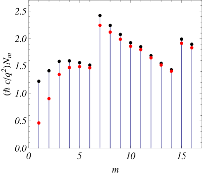
Figure 1: The number of the radiated quanta per period of the rotation on a given mode $m$ for the electron energy $E_{e}=2$ MeV and for the values of the parameters $\varepsilon_{1}=1$, $\varepsilon_{0}=3$, $\rho_{1}/\rho_{0}=1.2$. The black/red points correspond to the number of quanta evaluated by formula (32)/(33).

As it has been mentioned above, the number of the modes for a given $m$ increases with increasing $\rho_{1}$. For example, in the case $m=16$ one has $s_{m}=14$ for $\rho_{1}/\rho_{0}=2$ and $s_{m}=40$ for $\rho_{1}/\rho_{0}=4$ with the values of the other parameters being the same as those for figure 1. In order to illustrate the dependence on $s$, in figure 2 we present the number of the radiated quanta at a given mode, defined by (32), as a function of $\theta_{m,s}$ for $E_{e}=2$ MeV, $\varepsilon_{1}=1$, $\varepsilon_{0}=3$, $m=16$ and $\rho_{1}/\rho_{0}=4$. For large values $s$, the separation of two types of the modes is seen which are interlaced.

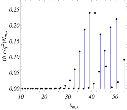
Figure 2: The number of the radiated quanta per period of the rotation on a given mode as a function of $\theta_{m,s}$. The values of the parameters are as follows: $E_{e}=2$ MeV, $\varepsilon_{1}=1$, $\varepsilon_{0}=3$, $m=16$ and $\rho_{1}/\rho_{0}=4$.

5 Radiation intensity outside a cylinder

For a charge rotating inside a dielectric cylinder, in Ref. [7] we have evaluated the average energy flux per unit time through the cylindrical surface of large radius $\rho$ ($\rho\gg\rho_{1}$) coaxial with the cylinder:

$$I_{\text{ex}}=\frac{2\pi}{T}\int_{0}^{T}dt\,\int_{-\infty}^{+\infty}dz\,\rho\mathbf{n}_{\rho}\cdot\mathbf{S}=\sum_{m=1}^{\infty}\int_{0}^{\pi}d\theta\,\frac{dI_{m}^{\text{(ex)}}}{d\theta},$$ (34)

where $\mathbf{n}_{\rho}$ is the unit vector along the radial direction and $\theta$ is the angle between the radiation direction and the axis of the cylinder. The expression for the angular density of the radiation intensity on a given harmonic $m$ with the frequency $m\omega_{0}$ is given by the expression

$$\frac{dI_{m}^{\text{(ex)}}}{d\theta}=\frac{q^{2}v^{2}m^{2}\omega_{0}^{2}\sqrt{\varepsilon_{1}}}{\pi^{2}c^{3}\rho_{1}^{2}}\sin\theta\left[|C_{m}^{(1)}-C_{m}^{(-1)}|^{2}+|C_{m}^{(1)}+C_{m}^{(-1)}|^{2}\cos^{2}\theta\right],$$ (35)

where we have defined

$$C_{m}^{(p)}=\frac{J_{m+p}(\lambda_{0}^{\text{(ex)}}\rho_{0})}{W_{m+p}^{J}}+p\lambda_{1}^{\text{(ex)}}H_{m}(\lambda_{1}^{\text{(ex)}}\rho_{1})\frac{J_{m+p}(\lambda_{0}^{\text{(ex)}}\rho_{1})}{2\alpha_{m}W_{m+p}^{J}}\sum_{l=\pm 1}\frac{J_{m+l}(\lambda_{0}^{\text{(ex)}}\rho_{0})}{W_{m+l}^{J}},$$ (36)

and

$$\lambda_{0}^{\text{(ex)}}=\frac{m\omega_{0}}{c}\sqrt{\varepsilon_{0}-\varepsilon_{1}\cos^{2}\theta},\;\lambda_{1}^{\text{(ex)}}=\frac{m\omega_{0}}{c}\sqrt{\varepsilon_{1}}\sin\theta.$$ (37)

The properties of the radiation corresponding to (35) are described in detail in [7] (see also Ref. [10] for a more general case of helical motion inside a dielectric cylinder). In particular, it was shown that under the Cherenkov condition for dielectric permittivity of the cylinder and the velocity of the particle image on the cylinder surface, strong narrow peaks are present in the angular distribution for the number of radiated quanta. At these peaks the radiated energy exceeds the corresponding quantity for a homogeneous medium by several orders of magnitude. The angular locations of the peaks are determined from the equation which is obtained from the equation determining the eigenmodes for the dielectric cylinder by the replacement $H_{m}(\lambda_{1}^{\text{(ex)}}\rho_{1})\rightarrow Y_{m}(\lambda_{1}^{\text{(ex)}}\rho_{1})$, where $Y_{m}(x)$ is the Neumann function. For the illustration, in figure LABEL:fig3 we plot the angular density of the number of the quanta radiated in the exterior region per period of the charge rotation,

$$\frac{dN_{m}^{\text{(ex)}}}{d\theta}=\frac{T}{\hbar m\omega_{0}}\frac{dI_{m}^{\text{(ex)}}}{d\theta},$$ (38)

with the radiation intensity given by (35). The corresponding parameters are as follows: $E_{e}=2$ MeV, $\varepsilon_{1}=1$, $\varepsilon_{0}=3$, $m=16$, $\rho_{1}/\rho_{0}=1.2$. The dashed curve corresponds to the synchrotron radiation in the vacuum in the absence of the dielectric cylinder ($\varepsilon_{0}=1$). We see the presence of the strong narrow peak at $\theta\approx 42.63$ (in degrees). The height of this peak is $\approx 463.4$ and the width $\approx 0.05$. At large distances from the cylinder for the total number of the radiated quanta one has $N_{m}^{\text{(ex)}}=1.748$. Note that for the number of quanta radiated on the eigenmodes of the cylinder we have $N_{m}=1.897$ (see figure 1). For the synchrotron radiation from an electron in the vacuum ($\varepsilon_{0}=1$) one has $N_{m}^{(0)}=0.352$. As it is seen, the presence of the cylinder considerably increases the radiation intensity.

Figure 3: The angular density of the number of the quanta radiated on the harmonic $m=16$ in the exterior region per period of the charge rotation as a function of $\theta$ (in degrees). The full curve is plotted for the values of parameters $E_{e}=2$ MeV, $\varepsilon_{1}=1$, $\varepsilon_{0}=3$, $m=16$, $\rho_{1}/\rho_{0}=1.2$. The dashed curve is for the radiation in the vacuum ($\varepsilon_{0}=1$).

Now we shall show that, in addition to the radiation corresponding to (34), in the exterior region we have also radiation fields localized near the surface of the dielectric cylinder. These fields are the tails of the eigenmodes for the dielectric cylinder. For this we need the expressions of the electric and magnetic fields in the exterior region. These fields can be presented in the form of the Fourier expansion (2), with the Fourier components of the magnetic field given by the expressions [7]

$$H_{ml} = \frac{i^{2-\sigma_{l}}qvk_{z}}{2\pi c}\sum_{p=\pm 1}p^{\sigma_{l}-1}B_{2,m}^{(p)}H_{m+p}(\lambda_{1}\rho),\;l=\rho,\phi,$$

$$H_{mz} = -\frac{qv\lambda_{1}}{2\pi c}\sum_{p=\pm 1}pB_{2,m}^{(p)}H_{m}(\lambda_{1}\rho),$$ (39)

where

$$B_{2,m}^{(p)}=\frac{J_{m+p}(\lambda_{0}\rho_{0})}{\rho_{1}W_{m+p}^{J}}+\frac{p\lambda_{1}J_{m+p}(\lambda_{0}\rho_{1})}{2\rho_{1}\alpha_{m}W_{m+p}^{J}}H_{m}(\lambda_{1}\rho_{1})\sum_{l=\pm 1}\frac{J_{m+l}(\lambda_{0}\rho_{0})}{W_{m+l}^{J}},$$ (40)

and the other notations are the same as in (4). For the electric field one has the expressions

$$E_{ml} = \frac{qvi^{1-\sigma_{l}}}{4\pi m\omega_{0}\varepsilon_{1}}\sum_{p=\pm 1}p^{\sigma_{l}}H_{m+p}(\lambda_{1}\rho)\sum_{j=\pm 1}j\left(\frac{m^{2}\omega_{0}^{2}}{c^{2}}\varepsilon_{1}+jk_{z}^{2}\right)B_{2,m}^{(jp)},$$

$$E_{mz} = -\frac{qiv\lambda_{1}k_{z}}{2\pi m\omega_{0}\varepsilon_{1}}\sum_{p=\pm 1}B_{2,m}^{(p)}H_{m}(\lambda_{1}\rho).$$ (41)

For a fixed value of $\rho>\rho_{1}$ and in the limit $z\rightarrow\infty$ the radiation fields are determined by the poles of the integrand in (2). These poles correspond to the zeros of the function $\alpha_{m}$. The fields are evaluated in a way similar to that we have used for the interior region. They are presented in the form (17), where

$$H_{m,s}^{l}(\rho) = k_{m,s}\sum_{p=\pm 1}p^{\sigma_{l}-1}B_{2,m,s}^{(p)}K_{m+p}(\lambda_{m,s}^{(1)}\rho/\rho_{1}),$$

$$H_{m,s}^{z}(\rho) = \frac{\lambda_{m,s}}{\rho_{1}}\sum_{p=\pm 1}B_{2,m,s}^{(p)}K_{m}(\lambda_{m,s}^{(1)}\rho/\rho_{1}),$$ (42)

for the magnetic field and

$$E_{m,s}^{l}(\rho) = \frac{(-1)^{\sigma_{l}-1}c}{2\varepsilon_{1}m\omega_{0}}\sum_{p=\pm 1}p^{\sigma_{l}}K_{m+p}(\lambda_{m,s}^{(1)}\rho/\rho_{1})\sum_{j=\pm 1}\left(\frac{m^{2}\omega_{0}^{2}}{c^{2}}\varepsilon_{1}+jk_{m,s}^{2}\right)B_{2,m,s}^{(jp)},$$

$$E_{m,s}^{z}(\rho) = \frac{c\lambda_{m,s}k_{m,s}}{\varepsilon_{1}\rho_{1}m\omega_{0}}\sum_{p=\pm 1}pB_{2,m,s}^{(p)}K_{m}(\lambda_{m,s}^{(1)}\rho/\rho_{1}),$$ (43)

for the electric field. In these expressions we have defined

$$B_{2,m,s}^{(p)}=\frac{\lambda_{m,s}^{(1)}J_{m+p}/K_{m}}{\left(V_{m}-pmu\right)J_{m}^{2}}\sum_{l=\pm 1}\frac{J_{m+l}(\lambda_{m,s}\rho_{0}/\rho_{1})}{V_{m}-lmu}.$$ (44)

As it is seen from (42) and (43), the radiation fields corresponding to the eigenmodes of the dielectric cylinder exponentially decay in the exterior region for $\rho/\rho_{1}\gg 1/\lambda_{m,s}^{(1)}$.

For the corresponding energy flux through a plane perpendicular to the axis of the cylinder,

$$I_{f}^{\text{(ex)}}=\int\limits_{\rho_{1}}^{\infty}d\rho\,\rho\int\limits_{0}^{2\pi}d\phi\,\mathbf{n}_{z}\cdot\mathbf{S},$$ (45)

one finds

$$I_{f}^{\text{(ex)}} = \sum_{m=1}^{\infty}I_{f,m}^{\text{(ex)}}=\frac{q^{2}v^{2}\rho_{1}^{2}}{8\varepsilon_{1}\omega_{0}}\sum_{m=1}^{\infty}\sum_{s}\frac{k_{m,s}\lambda_{m,s}^{(1)2}J_{m}^{-4}}{m\alpha_{m}^{\prime 2}(k_{m,s})K_{m}^{2}}\left[\sum_{l=\pm 1}\frac{J_{m+l}(\lambda_{m,s}\rho_{0}/\rho_{1})}{V_{m}-lmu}\right]^{2}$$ (46)

$$\times\sum_{p=\pm 1}\frac{J_{m+p}}{V_{m}-pmu}\left[\left(\frac{m^{2}\omega_{0}^{2}}{c^{2}}\varepsilon_{1}+k_{m,s}^{2}\right)\frac{J_{m+p}}{V_{m}-pmu}-\frac{\lambda_{m,s}^{(1)2}}{\rho_{1}^{2}}\frac{J_{m-p}}{V_{m}+pmu}\right]$$

$$\times\left[K_{m+p}^{\prime 2}-\left(1+\frac{(m+p)^{2}}{\lambda_{m,s}^{(1)2}}\right)K_{m+p}^{2}\right].$$

Now it can be explicitly checked that one has the relation $I_{m}=2\left(I_{f,m}^{\text{(in)}}+I_{f,m}^{\text{(ex)}}\right)$.

In figure 4 we have plotted the number of the radiated quanta per period of the rotation on a given mode $m$ for different values of $m$. The values of the parameters are as follows: $E_{e}=2$ MeV, $\varepsilon_{1}=1$, $\varepsilon_{0}=3$, $\rho_{1}/\rho_{0}=1.2$. The black points correspond to the radiation in the exterior region at latge distances from the cylinder, $N_{m}^{\text{(ex)}}=\int_{0}^{\pi/2}d\theta(dN_{m}^{\text{(ex)}}/d\theta)$ (see ()38), and the red points are for the radiation on the eigenmodes of the dielectric cylinder, $N_{m}^{\text{(in)}}=\sum_{s}N_{m,s}$ (see (32)). For the comparison with the synchrotron radiation in the vacuum, in figure 5, for the same values of the parameters, we plot the total number of the radiated quanta, $N_{m}=N_{m}^{\text{(in)}}+N_{m}^{\text{(ex)}}$, in the presence (black points) and in the absence (red points) of the dielectric cylinder. As it is seen from these graphs, the presence of the cylinder essentially increases the radiation intensity.

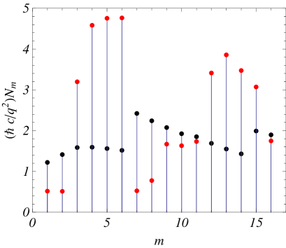
Figure 4: The number of the radiated quanta per period of the rotation on a given mode $m$ for different values of $m$ and for the values of the parameters $E_{e}=2$ MeV, $\varepsilon_{1}=1$, $\varepsilon_{0}=3$, $\rho_{1}/\rho_{0}=1.2$. The black points correspond to the radiation in the exterior region and the red points are for the radiation emitted on the eigenmodes of the dielectric cylinder.

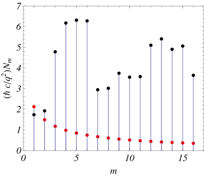
Figure 5: The total number of the radiated quanta, $N_{m}=N_{m}^{\text{(in)}}+N_{m}^{\text{(ex)}}$, in the presence (black points) and in the absence (red points) of the dielectric cylinder. The values of the parameters are the same as those for figure 4.

We have considered the energy loss for a particle rotating in a medium due to the synchrotron radiation. A point which deserves a separate investigation is the role of the other processes of the particle interaction with the medium. In particular, they include ionization energy losses, particle bremsstrahlung in media, and the multiple scattering (see, for instance, [24, 25, 26]). The relative role of these processes depends on the particle energy and characteristics of the medium and has been shortly discussed in [12]. An interesting possibility of escaping ionization losses in the medium was indicated in [27], where it was argued that a narrow empty channel along the particle trajectory in the solid dielectric does not affect the radiation intensity if the channel radius is less than the radiation wavelength.

6 Conclusion

We have investigated the synchrotron radiation from a charged particle rotating inside a dielectric cylinder surrounded by a homogeneous medium. The radiation intensity in the exterior medium at large distances from the cylinder has been considered previously in [7] and here we were mainly concerned with the radiation propagating inside the cylinder. The electromagnetic fields inside the cylinder are presented in the form of the Fourier expansion (3), where the Fourier components for the magnetic and electric fields are given by the expressions (4) and (9). The radiation parts of the fields propagating inside the cylinder are determined by the contribution of the poles of the Fourier components. These poles correspond to the zeros of the function $\alpha_{m}$ given by (7). The latter are the bound modes of the dielectric cylinder and are determined from the equation (13). The electromagnetic fields for the radiation propagating inside the cylinder are presented in the form (17) with the expressions (18) and (21) for separate components of the magnetic and electric fields.

The radiation intensity inside the cylinder is investigated in Section 4. Firstly we have evaluated the work done by the radiation field on the charged particle. The radiation intensity evaluated in this way is given by the expression (23). In the limit when the radius of the cylinder goes to infinity this expression reduces to the formula for the intensity of the synchrotron radiation in a homogeneous medium with dielectric permittivity $\varepsilon_{0}$. Further, we have evaluated the energy flux through the cross-section of the cylinder. The radiation intensity evaluated in this way is given by the expression (31). A numerical example for the radiation intensities evaluated in two different ways is presented in figure 1. As it is seen, the intensities evaluated by the work done on the charge and by the flux through the cross-section do not coincide. In Section 5 we show that the reason for this difference is that for the eigenmodes of the dielectric cylinder there is also energy flux in the exterior region located near the surface of the cylinder.

The radiation field in the exterior region consists of two parts. The first one corresponds to the radiation propagating at large distances from the cylinder. The angular density of the corresponding radiation intensity on a given harmonic $m$ is given by the formula (35). For large values of $m$ and under the Cherenkov condition for dielectric permittivity of the cylinder and the velocity of the particle image on the cylinder surface, strong narrow peaks appear in the angular distribution for the radiation intensity. An example is given in figure LABEL:fig3. The second part of the radiation field in the exterior region corresponds to the modes of the dielectric cylinder. The corresponding fields are located near the surface of the cylinder and are given by the formula (2), with the Fourier components of the magnetic and electric fields given by the expressions (39) and (41). These fields exponentially decay at distances from the cylinder surface larger than the radiation wavelength. The energy flux in the exterior region corresponding to the eigenmodes of the cylinder is given by the expression (46). We have explicitly checked that the radiation intensity evaluated by the work done by the radiation field on the charged particle is equal to the radiation intensity evaluated by the energy flux through the plane perpendicular to the cylinder axis if we take into account the contribution of the radiation field in the exterior region.

As we have seen in the present paper, the insertion of a dielectric waveguide provides an additional mechanism for tuning the characteristics of the synchrotron radiation by choosing the parameters of the waveguide. The radiated energy inside the cylinder is redistributed among the cylinder modes and, as a result, the corresponding spectrum differs significantly from the homogeneous medium or free-space results. This change is of special interest in the low-frequency range where the distribution of the radiation energy among small number of modes leads to the enhancement of the spectral density for the radiation intensity. The radiation emitted on the waveguide modes propagates inside the cylinder and the waveguide serves as a natural collector for the radiation. This eliminates the necessity for focusing to achieve a high-power spectral intensity. The geometry considered here is of interest also from the point of view of generation and transmitting of waves in waveguides, a subject which is of considerable practical importance in microwave engineering and optical fiber communications.

References

• [1] A.A. Sokolov, I.M. Ternov, Radiation from Relativistic Electrons (New York: AIP Press,1986 ).
• [2] Synchrotron Radiation Theory and Its Development, edited by V.A. Bordovitsyn (World Scientific, Singapore, 1999).
• [3] A. Hofman, The Physics of Sinchrotron Radiation (Cambridge University Press, Cambridge, 2004).
• [4] L.Sh. Grigoryan, A.S. Kotanjyan, A.A. Saharian, Izv. Akad. Nauk Arm. Fiz. 30, 239 (1995) [Sov. J. Contemp. Phys. 30, 1 (1995)]..
• [5] A.S. Kotanjyan, H.F. Khachatryan, A.V. Petrosyan, A.A. Saharian, Izv. Akad. Nauk Arm. Fiz. 35, 115 (2000) [Sov. J. Contemp. Phys. 35, 1 (2000)].
• [6] A.S. Kotanjyan, A.A. Saharian, Izv. Akad. Nauk Arm. Fiz. 36, 310 (2001) [Sov. J. Contemp. Phys. 36, 7 (2001)].
• [7] A. S. Kotanjyan, A. A. Saharian, Izv. Akad. Nauk Arm. Fiz. 37, 263 (2002) [J. Contemp. Phys. 37, 263 (2002)].
• [8] A.S. Kotanjyan, A.A. Saharian, Mod. Phys. Lett. A 17, 1323 (2002).
• [9] A.S. Kotanjyan, Nucl. Instrum. Methods B201, 3 (2003).
• [10] A.A. Saharian, A.S. Kotanjyan, J. Phys. A 38, 4275 (2005).
• [11] A.A. Saharian, A.S. Kotanjyan, M.L. Grigoryan, J. Phys. A 40, 1405 (2007).
• [12] A.A. Saharian, A.S. Kotanjyan, J. Phys. A 40, 10641 (2007).
• [13] S.R. Arzumanyan, L.Sh. Grigoryan, H.F. Khachatryan, A.S. Kotanjyan, A.A. Saharian, Nucl. Instrum. Methods B266, 3703 (2008).
• [14] A.A. Saharian, A.S. Kotanjyan, J. Phys. A 42, 135402 (2009).
• [15] S.R. Arzumanian, L.Sh. Grigoryan, Kh.V. Kotanjyan, A.A. Saharian, Izv. Akad. Nauk Arm. Fiz. 30, 106 (1995) [Sov. J. Contemp. Phys. 30, 12 (1995)].
• [16] L.Sh. Grigoryan, H.F. Khachatryan, S.R. Arzumanyan, Izv. Akad. Nauk Arm. Fiz. 33, 267 (1998) [Sov. J. Contemp. Phys. 33, 1 (1998)], cond-mat/0001322.
• [17] L.Sh. Grigoryan, H.F. Khachatryan, S.R. Arzumanyan, Izv. Akad. Nauk Arm. Fiz. 37, 327 (2002) [Sov. J. Contemp. Phys. 37, 1 (2002)].
• [18] L.Sh. Grigoryan, H.F. Khachatryan, S.R. Arzumanyan, M.L. Grigoryan, Nucl. Instrum. Methods B 252, 50 (2006).
• [19] J.D. Jackson, Classical Electrodynamics (John Wiley & Sons, 1998).
• [20] Handbook of Mathematical Functions, ed. M. Abramowitz, I. A. Stegun (New York: Dover, 1972).
• [21] V.N. Tsytovich, Westnik MGU 11, 27 (1951) (in Russian).
• [22] K. Kitao, Prog. Theor. Phys. 23, 759 (1960).
• [23] V.P. Zrelov, Vavilov–Cherenkov Radiation and its Applications in High-Energy Physics (Moscow: Atomizdat, 1968) (in Russian).
• [24] M.L. Ter-Mikaelian, High Energy Electromagnetic Processes in Condensed Media (New York: Wiley, 1972).
• [25] A.I. Akhiezer, N.F. Shul’ga, High Energy Electrodynamics in Matter (London: Gordon and Breach, 1996).
• [26] P. Rullhusen, X. Artru, P. Dhez, Novel Radtiation Sources Using Relativistic Electrons (Singapore: World Scientific, 1998)
• [27] B.M. Bolotovskii, Sov. Phys. Usp. 4, 781 (1961).