Replica Field Theory of the Dynamical Transition in Glassy Systems

Abstract

The critical behaviour of the dynamical transition of glassy system is controlled by a Replica Symmetric action with $n=1$ replicas. The most divergent diagrams in the loop expansion correspond at all orders to the solutions of a stochastic equation leading to perturbative dimensional reduction. The theory describe accurately numerical simulations of mean-field models.

More that twenty years ago it was recognized KTW that a certain class of mean-field spin-glass models (techically speaking, those where replica symmetry is broken at one step) displays the same dynamical behaviour predicted by the Mode-Coupling Theory (MCT) of glasses MCT . This has motivated a great deal of research BBRFOT and many believe that there is an intrinsic analogy between these two classes of systems.

Lowering the temperature, these models display two transitions. At the dynamical transition temperature $T_{d}$ the paramagnetic equilibrium state abruptly splits into a number of states that is exponentially large in the size of the system. Correspondingly the equilibrium dynamics displays the well known MCT phenomenology. At a static transition temperature $T_{s}<T_{d}$ the number of equilibrium states is no longer exponential and this is strongly reminiscent of the entropy crisis which is supposed to happen at the Kauzmann temperature in glasses. Between $T_{d}$ and $T_{s}$, the entropy crisis supplemented by nucleation arguments is used to explain the observed super-Arrhenius slowing down of the dynamics and there are currently many efforts to verify this scenario.

On the other hand MCT offers a good description of the early stages of the dynamical slowing down and in this Letter we discuss finite-size and finite-dimensional effects at $T_{d}$, i.e. at the Mode-Coupling temperature. The dynamical transition is characterized by a diverging correlation length FPchi4 ; BB and therefore it is natural to ask which are the mean-field critical exponents, what is the upper critical dimension $d_{u}$ above which they are valid, and how they are renormalized below. It is worth noticing that we should rather speak of pseudo-critical exponents because, due to activated effects, the dynamical transition is bound to disappear or rather to become a cross-over in finite dimension, much as in more conventional metastable phenomena.

In spin-glass models the local variables are usually Ising spins $s_{i}=\pm 1$ and the relevant order parameter is the overlap between different equilibrium configurations $q(\sigma,\tau)\equiv N^{-1}\sum_{i}\sigma_{i}\tau_{i}$. The same order parameter can be studied for liquids in a lattice gas representation. It is well known that in mean-field models the dynamical transition can be located through a static potential $V(q)$ defined as the average free-energy cost of imposing that the system stays at an overlap $q$ from a fixed equilibrium configuration FP . The potential has a minimum at the equilibrium value of the overlap ($q=0$ in the absence of external fields), but below $T_{d}$ a secondary minimum appears at a higher value, $q=q_{d}$, in the mean-field theory of the problem. Using the replica method the potential $V(q)$ can be expressed as a field theory of an action of a replicated order parameter that is an $n\times n$ overlap matrix $q_{ab}$ with $q_{aa}=0$ (to be continued analytically to $n\to 0$). The paramagnetic solution is $q_{ab}=0$ down to $T_{s}$, however at $T_{d}$ a solution appears with $q_{ab}=q_{d}$ inside an $m\times m$ block with $m=1$ (analytic continuation) FP ; Monasson . We want to study the loop expansion around the latter solution which encodes the presence of an exponential number of states. Such an expansion can be simplified noticing that only the modes with diverging Gaussian fluctuations are relevant for critical behaviour, while all the others can be integrated out. Since $T_{d}$ is essentially a spinodal point for the $m=1$ solution, it is natural to assume that the only critical variables $q_{ab}$ are those inside the $m\times m$ block. We thus reach the conclusion that the relevant field-theory of the problem in the Ginzburg-Landau sense is a cubic Replica-Symmetric (RS) field theory with $n=1$ replicas:

$${\mathcal{L}}={1\over 2}\int dx\left(\sum_{ab}(\nabla\phi_{ab})^{2}+m_{1}\sum_{ab}\phi_{ab}^{2}+m_{2}\sum_{abc}\phi_{ab}\phi_{ac}+m_{3}\sum_{abcd}\phi_{ab}\phi_{cd}\right)-{1\over 6}\omega_{1}\sum_{abc}\phi_{ab}\phi_{bc}\phi_{ca}-{1\over 6}\omega_{2}\sum_{ab}\phi_{ab}^{3}\;,$$ (1)

where $\phi_{ab}$ is the difference between the actual value of the order parameter $q_{ab}$ and its mean-field value $q_{d}^{MF}$ and $\phi_{aa}=0$. In the above expression we have retained only the cubic terms relevant for critical behaviour. In the critical region we have $m_{1}\propto(T_{d}^{MF}-T)^{1/2}$, where $T_{d}^{MF}$ is the dynamical temperature in the mean-field approximation. The corresponding dressed propagators can be associated to the following physical quantities:

$$G_{1}(x,y)\equiv\langle\phi_{ab}(x)\phi_{ab}(y)\rangle_{c}=\overline{\langle s_{x}s_{y}\rangle^{2}}-\overline{\langle s_{x}\rangle^{2}}\ \overline{\langle s_{y}\rangle^{2}}$$ (2)

$$G_{2}(x,y)\equiv\langle\phi_{ab}(x)\phi_{ac}(y)\rangle_{c}=\overline{\langle s_{x}s_{y}\rangle\langle s_{x}\rangle\langle s_{y}\rangle}-\overline{\langle s_{x}\rangle^{2}}\ \overline{\langle s_{y}\rangle^{2}}$$ (3)

$$G_{3}(x,y)\equiv\langle\phi_{ab}(x)\phi_{cd}(y)\rangle_{c}=\overline{\langle s_{x}\rangle^{2}\langle s_{y}\rangle^{2}}-\overline{\langle s_{x}\rangle^{2}}\ \overline{\langle s_{y}\rangle^{2}}$$ (4)

In the r.h.s. of the above expressions the overline means averages over the quenched disorder and over the exponential number of states in which the paramagnetic state splits at $T_{d}$, while the various angle brackets mean thermal averages computed inside the same equilibrium state. We can also consider connected correlations w.r.t. the thermal noise inside the same state, by making linear combinations of $G_{1}$, $G_{2}$ and $G_{3}$ that cancel the last term in eqs.(2–4), e.g.

$$G_{SG}(x,y) \equiv G_{1}-2G_{2}+G_{3}=\overline{(\langle s_{x}s_{y}\rangle-\langle s_{x}\rangle\langle s_{y}\rangle)^{2}}\;,$$

$$G_{th}(x,y) \equiv G_{1}-G_{2}\;,\quad G_{q}(x,y)\equiv G_{1}-G_{3}$$ (5)

While these connected correlations describe fluctuations inside a given state, $G_{1}$, $G_{2}$ and $G_{3}$ yield fluctuations between different states, and will be called disconnected correlations in the following.

We note that the above theory can be used also to describe systems without quenched disorder, notably structural glasses. The key requirement is that there is an exponential number of equilibrium states and in this case the overline have to be interpreted just as an average over them. This so-called self-induced disorder is supposed to be the bridge between spin-glasses and glasses and it is the reason why the replica method can be successfully applied to glasses MP ; SZ .

At the Gaussian level, fluctuations are controlled by the three eigenvalues of the quadratic part of $\mathcal{L}$: replicon $r_{R}$, longitudinal $r_{L}$ and anomalous $r_{A}$ TDP . Degeneracies occurs at special values of $n$: $n=0\rightarrow r_{A}=r_{L}$, $n=1\rightarrow r_{L}=r_{R}$, $n=2\rightarrow r_{A}=r_{R}$. We have found that, as a consequence of the degeneracy at $n=1$ between the replicon and longitudinal eigenvalues, a double pole appears in the bare propagators. Switching to momentum representation the leading divergent behaviour is given by:

$$G_{1}(k) = {2\,a\over(k^{2}+r_{R})^{2}}-{1\over k^{2}+r_{R}}+{2\over r_{A}}\;,$$

$$G_{2}(k) = {2\,a\over(k^{2}+r_{R})^{2}}-{3\over k^{2}+r_{R}}+{3\over r_{A}}\;,$$

$$G_{3}(k) = {2\,a\over(k^{2}+r_{R})^{2}}-{4\over k^{2}+r_{R}}+{4\over r_{A}}\;,$$

where $r_{R}=r_{L}=2m_{1}$ and $a\equiv\lim_{n\rightarrow 1}(r_{R}-r_{L})/(n-1)=-2m_{2}-2m_{3}$. Note that $r_{A}$ is not critical and remains non-zero. The presence of an unexpected double pole is similar to what happens in the Random Field Ising Model (RFIM) DDG . Another feature of the above expressions that resembles the RFIM is the fact that any connected correlation diverges instead with a single pole. It is well known that the perturbative loop expansion of the RFIM is the same of a stochastic equation PS1 : quite surprisingly we have found that this property is also shared by the RS field theory with $n=1$. We stress that in the literature similar loop expansions are usually limited to the first few orders DDG ; TDP for general values of $n$ because for each diagram one has to perform a complex summation over replica indices. Therefore it is remarkable that in the case $n=1$ one controls the loop expansion at all orders. The most divergent diagrams in the loop expansion of the theory (1) corresponds at all orders to the solution of the following cubic equation in presence of a quenched Gaussian random field $h(x)$

$$-\Delta\phi+r_{R}\phi+\omega\phi^{2} = h\;,$$ (6)

$$\text{with}\quad\quad[h(x)h(y)]_{h} = 2\,a\,\delta(x-y)\;.$$

There is an unique cubic constant $\omega=\omega_{2}-\omega_{1}$ and $[\dots]_{h}$ means average over the random field. The precise meaning of the equivalence is that the most divergent diagrams in the loop expansion of $G_{1}(x,y)$, $G_{2}(x,y)$, $G_{3}(x,y)$ coincide to all orders with the loop expansion of $[\phi(x)\phi(y)]_{h}$ where $\phi$ is solution to eq. (6). The correspondence also holds at the level of the less divergent connected correlations functions and we have:

$$G_{SG}=[\phi h]_{h}\,,\;G_{th}=2[\phi h]_{h}\,,\;G_{q}=3[\phi h]_{h}$$ (7)

The stochastic equation (6) leads to a simple physical interpretation: critical behavior is controlled by the random field fluctuations from state-to-state. The diagrammatic analisys shows that the upper critical dimension is $d_{u}=8$ and not the naive expectation 6. Furthermore the mapping to the stochastic equation implies a perturbative dimensional reduction PS1 , suggesting that the critical exponents are the same of the pure model in dimension $D-2$. In the RFIM dimensional reduction does not hold because of non perturbative effects PS1 while it does hold for branched polymers PS2 . There is no general recipe to know if it holds or not and we will not further comment on this point.

At the mean-field level the theory predicts critical exponents different from those of a standard cubic theory. Remarkably the predictions of the latter have been found to disagree with numerical simulations in a recent study SBBB . In mean-field it is natural to study the critical behavior of integrated quantities diverging at the critical point, like the susceptibilities $\chi_{\bullet}\equiv N^{-1}\sum_{x,y}G_{\bullet}(x,y)$, where $N$ is the system size. As usual the loop expansion can be recast formally in order to deal with divergences at criticality, and the result is that disconnected susceptibilities diverge as $N^{1/2}$, while connected susceptibilities diverge as $N^{1/4}$. However the prefactors are expressed as series with all positive coefficients, and are not resummable. This can be seen also noticing that the stochastic equation (6) does not admit a real solution for a sufficiently negative field meaning that the averages $[\dots]_{h}$ are not well defined beyond perturbation theory. This is precisely what we were expecting because we are dealing with metastable states that are intrinsically ill-defined at the critical temperature. On the other hand, dynamics is always well defined, and allow us to access the critical region (e.g. in numerical simulations) to test the above critical exponents.

We have studied numerically the dynamics at $T_{d}$, using a mean-field model of $N$ Ising spins $s_{i}=\pm 1$, interacting by 3-spin couplings ($J_{ijk}=\pm 1$), randomly chosen such that each spin participates exactly to $z=8$ interactions. Starting from an equilibrated configuration, we measured the overlap $C(t)=\sum_{i=1}^{N}s_{i}(0)s_{i}(t)/N$ between the initial configuration and the configuration at time $t$. Below $T_{d}$ the initial condition determines the state in which the system will remain trapped along the dynamics. The fluctuations of $C(t)$ are called $\chi_{4}(t)$ in the glass literature FPchi4 . However, according to our results it is crucial to distinguish between disconnected and connected fluctuations; so we write $\chi_{4}(t)=\chi_{het}(t)+\chi_{th}(t)$ with

$$\chi_{het}(t) \equiv N\left(\overline{\langle C(t)\rangle^{2}}-\overline{\langle C(t)\rangle}^{2}\right)\;,$$ (8)

$$\chi_{th}(t) \equiv N\;\overline{\langle C(t)^{2}\rangle-\langle C(t)\rangle^{2}}\;.$$ (9)

In the $t\to\infty$ limit, we have that $\chi_{het}(t)\to\chi_{2}\equiv N^{-1}\sum_{x,y}G_{2}(x,y)$, $\chi_{th}(t)\to\chi_{th}\equiv N^{-1}\sum_{x,y}G_{th}(x,y)$ and $\chi_{4}(t)\to\chi_{1}\equiv N^{-1}\sum_{x,y}G_{1}(x,y)$. This connection allow us to test the above scaling predictions through dynamical measurements.

Numerically we work on the Nishimori line, such that the starting configuration with all $s_{i}(0)=1$ is an equilibrium configuration NishiInit . Therefore for each sample we consider just one of the exponentially many typical states and averages between different states are obtained changing the sample. Averages are computed by a number of samples (states) $N_{S}$ such that $NN_{S}=3\cdot 10^{7}$ and with 2 real replicas per sample evolving with different thermal noises. The dynamics exhibits the MCT phenomenology. In particular above $T_{d}$ the average correlation $C_{av}(t)\equiv\overline{\langle C(t)\rangle}$ relaxes to zero in a two-step fashion. On the time scale $t_{\beta}$ of the $\beta$ regime $C_{av}(t)$ remains around a plateau value $C_{p}$, while one the larger time scale $t_{\alpha}$ of the $\alpha$ regime it decays to zero. Both the two time-scales diverge at $T_{d}$ and the system remains in the state selected by the initial configuration. The analytical solution of the model MRT gives $T_{d}=1.3420(5)$ and $C_{p}=0.750(5)$. Even at $T=T_{d}$, due to finite size effects, $C_{av}(t)$ eventually decays to zero although on time scales diverging with the system size. In present context we do not want to discuss the behaviour of these time scales and we find convenient to consider reparameterized quantities $\chi_{het}(C_{av})$ and $\chi_{th}(C_{av})$ HKproc . We may distinguish three regions.

The perturbative region corresponds to $C_{av}>C_{p}$. It is reached in times of order $O(1)$, such that fluctuations are themself $O(1)$ and admit a regular expansion in powers of $1/N$. Using rather natural finite-time-scaling arguments one can match these dynamical perturbative series with the perturbative series of the statics generated by action (1). It can be argued that the coefficients of the various terms in the expansions diverge with the same power of $\delta C\equiv(C_{av}-C_{p})$ of the corresponding static quantity. In particular the most divergent terms at any order are given by

$$\chi_{het}(C_{p}+\delta C) = {1\over\delta C^{2}}\sum_{k=0}^{\infty}{c_{k}\over(N\delta C^{4})^{k}}\;,$$ (10)

$$\chi_{th}(C_{p}+\delta C) = {1\over\delta C}\sum_{k=0}^{\infty}{d_{k}\over(N\delta C^{4})^{k}}\;.$$ (11)

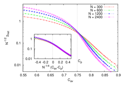
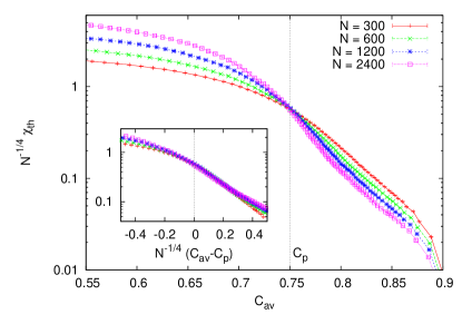
Figure 1: (color online) Rescaled disconnected susceptibility $N^{-1/2}\chi_{het}(C_{av})$ (top) and rescaled connected susceptibility $N^{-1/4}\chi_{th}(C_{av})$ (bottom). The curves for different system sizes cross at the analytically known plateau value $C_{p}=0.75$. The insets show the same data rescaled horizontally according to the scaling variable $x=N^{-1/4}(C_{av}-C_{p})$, leading to a very good data collapse.

The scaling region corresponds to values of $C_{av}(t)$ near $C_{p}$. This region is explored on a time scale diverging with the system size and we expect diverging fluctuations. According to the above perturbative series the scaling region corresponds to $\delta C=O(N^{-1/4})$, with the following scaling laws

$$\chi_{het}(C_{p}+N^{-1/4}x) = N^{1/2}f_{het}(x)\;,$$ (12)

$$\chi_{th}(C_{p}+N^{-1/4}x) = N^{1/4}f_{th}(x)\;,$$ (13)

where the two scaling functions $f_{het}(x)$ and $f_{th}(x)$ go to zero for $x\rightarrow+\infty$ and diverge for $x\rightarrow-\infty$. The above perturbative series provide their asymptotic expansion for $x\rightarrow\infty$: at leading order $f_{het}(x)\sim x^{-2}$ and $f_{th}(x)\sim x^{-1}$. The numerical data are in very good agreement with the expected behaviour, see Fig. 1.

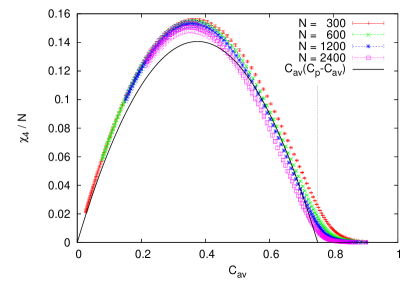
Figure 2: Normalized disconnected susceptibility $\chi_{4}$ in the $\alpha$ regime, $C_{av}<C_{p}$.

The $\alpha$ regime corresponds to $0<C_{av}<C_{p}$ and we can not use any perturbative information here. In this region our numerical data are close to the form $\chi_{4}(C_{av})=NC_{av}(C_{p}-C_{av})$, see Fig. 2, which would hold if, for any initial configuration and thermal noise, the relaxation consisted in a sharp jump from the plateau value $C_{p}$ to the value for uncorrelated configurations, $C=0$.

It is worth noticing that it is far from trivial that the exponents predicted in perturbation theory can be actually observed in the critical region. Indeed if non-perturbative effects were also present on the same time scale they would wash out the perturbative results. Our results suggest that non-perturbative effects appear instead on a larger time scale. The time scale of the critical region diverges with the system size as $N^{1\over 4a}$ and a reasonable possibility is that the time scale of the $\alpha$ regime scales like $N^{{1\over 4a}+{1\over 4b}}$, where $a$ and $b$ are the dynamical MCT exponents of the $\beta$ regime. The results of the static theory can be used to safely infer other properties of critical dynamics in the early $\beta$ regime. In particular, for $\tau\equiv T-T_{d}>0$, we have a $\beta$-like regime for short time, $t<t_{\beta}=O(\tau^{-1/2a})$, where the following scaling laws should hold

$$\chi_{het}(t)=\frac{1}{\tau}\,g_{het}(t/t_{\beta})\;,\quad\chi_{th}(t)=\frac{1}{\sqrt{\tau}}\,g_{th}(t/t_{\beta})\;.$$ (14)

Correspondingly, we have $\chi_{4}(t)\propto\chi_{het}(t)\propto t^{2a}$ and $\chi_{th}(t)\propto t^{a}$ at finite times. It could be that one is able by means of matching arguments and numerical observation to access also the late $\beta$ regime and the $\alpha$ regime. We choose however not to discuss this point because we think that a satisfactory understanding of the $\alpha$ regime shall include an analitycal treatment of non-perturbative effects.

References

- (1) T.R. Kirkpatrick and D. Thirumalai, Phys. Rev. Lett. 58, 2091 (1987); Phys. Rev. B 36, 5388 (1987); T.R. Kirkpatrick, D. Thirumalai and P.G. Wolynes, Phys. Rev. A 40, 1045 (1989).
- (2) W. Gotze, Complex Dynamics of Glass-Forming Liquids (Oxford University Press, Oxford, 2009).
- (3) G. Biroli and J.-P. Bouchaud, The Random First-Order Transition Theory of Glasses: a critical assessment, arXiv:0912.2542 (2009).
- (4) S. Franz and G. Parisi, J. Phys. Cond. Mat. 12, 6335 (2000). C. Donati, S. Franz, G. Parisi and S.C. Glotzer, J. of Non-Cryst. Solids 307-310, 215 (2002).
- (5) J. Bouchaud and G. Biroli, Europhys. Lett. 67, 21 (2004).
- (6) S. Franz, G. Parisi, J. Phys. I (France) 5, 1401 (1995); Phys. Rev. Lett. 79 2486 (1997); Physica A 261, 317 (1998).
- (7) R. Monasson, Phys. Rev. Lett. 75, 2847 (1995).
- (8) M. Mezard and G. Parisi, Replicas and Glasses, arXiv:0910.2838 (2009).
- (9) G. Szamel, Europhys. Lett. 91, 56004 (2010).
- (10) T. Temesvari, C. De Dominicis and I. R. Pimentel, Eur. Phys. J. B 25, 361 (2002).
- (11) C. De Dominicis and I. Giardina, Random Fields and Spin Glasses (Cambridge University Press, Cambridge, 2006).
- (12) G. Parisi and N. Sourlas, Phys. Rev. Lett. 43, 744 (1979).
- (13) J.L. Cardy, Phys. Lett. B 125, 470 (1983); Physica D 15, 123 (1985).
- (14) G. Parisi and N. Sourlas, Phys. Rev. Lett. 46, 871 (1981).
- (15) T. Sarlat, A. Billoire, G. Biroli and J.-P. Bouchaud, J. Stat. Mech. P08014 (2009).
- (16) Y. Ozeki, J. Phys. A: Math. Gen. 28, 3645 (1995). F. Krzakala and L. Zdeborova, J. Chem. Phys. 134, 034513 (2011).
- (17) A. Montanari and F. Ricci-Tersenghi, Eur. Phys. J. B 33, 339 (2003); Phys. Rev. B 70, 134406 (2004).
- (18) S. Franz, G. Parisi, F. Ricci-Tersenghi and T. Rizzo, preprint arxiv:1008:0996 (2010).