Structure and direct decay of Giant Monopole Resonances

Abstract

We study structure and direct decay of the Giant Monopole Resonance (GMR) at the RPA level using the Time-Dependent Energy Density Functional method in the linear response regime in a few doubly-magic nuclei. A proper treatment of the continuum, through the use of large coordinate space, allows for a separation between the nucleus and its emitted nucleons. The microscopic structure of the GMR is investigated with the decomposition of the strength function into individual single-particles quantum numbers. A similar microscopic decomposition of the spectra of emitted nucleons by direct decay of the GMR is performed. In this harmonic picture of giant resonance, shifting every contribution by the initial single-particle energy allows to reconstruct the GMR strength function. The RPA residual interaction couples bound 1-particle 1-hole states to unbound ones, allowing for the total decay of the GMR. In this article, we then intend to get an understanding of the direct decay mechanism from coherent one-particle-one-hole superpositions, while neglecting more complex configurations. Time-dependent beyond mean-field approaches should be use, in the future, to extend this method.

I Introduction

Atomic nuclei are known to exhibit a wide range of collective excitations Boh75 . Amongst them, giant resonances (GRs) are of particular interest in our understanding of collective motion in nuclei. Macroscopically, they are associated to high energy modes of small amplitude vibration of the entire nucleus. Microscopically, they can be modeled, in the harmonic picture, by coherent superpositions of one-particle one-hole (1p1h) excitations Boh75 , although more complex configurations such as 2p2h excitations are necessary to reproduce their experimental widths Har01 .

The width of GRs has three components: the escape width ($\Gamma^{\uparrow}$), the Landau damping ($\Gamma^{L}$), and the spreading width ($\Gamma^{\downarrow}$). The escape width is due to the GR decay by particle emission. Its microscopic origin is the coupling of the correlated $1p1h$ states to the continuum. Landau damping occurs due to a one-body coupling to non-coherent $1p1h$ states pin66 . The spreading width is due to the residual interaction coupling $1p1h$ states to $2p2h$ states. The $2p2h$ states can also couple to $3p3h$ states and more complex $npnh$ configurations until an equilibrated system is reached.

The principal approaches to treat collective vibrations in terms of 1p1h constituents are the Random Phase Approximation (RPA) boh53 and its relativistic extensions lhu89 ; oak92 ; vre97 . The RPA equations can be obtained as a linearization of the time-dependent Hartree-Fock (TDHF) equation Rin80 . The recent increase of computational power allowed for the development of realistic TDHF codes able to follow the dynamics of $\sim 500$ interacting nucleons gol09 ; ked10 . As a result, several modern TDHF codes have been used to investigate the linear response to vibrational excitations Uma05 ; Mar05 ; Nak05 ; fra12 (see also Ref. sim12 for a recent review). In addition, pairing correlations can be included within the Quasiparticle-RPA (QRPA) Rin80 ; Bla86 , which has been widely used to study various GR strength distributions, either by solving the QRPA equations (see, e.g., Refs. eng99 ; Kha02 ; kha04 ; fra05 ; per08 ; yos11 ), or with small amplitude real time calculations Ave08 ; Eba10 ; ste11 ; has12 .

The main drawback of these approaches is the limitation to the independent (quasi)particle picture which prevents the inclusion of more complex configurations. In particular, the spreading width cannot be determined at the RPA level because 2p2h configurations are neglected. Several approaches have then been considered to go beyond the independent (quasi)particle description of quantum vibrations. The inclusion of (quasi)particle-phonon coupling bor81 ; kam04 has shown to be very efficient to reproduce the width of giant resonances, e.g., in tin isotopes tse09 . The extended-TDHF approach Lac04 , and the time-dependent density-matrix theory Toh01 , both lead to the inclusion of 2p2h configurations in their small amplitude limit thanks to collisional damping. Similarly, the RPA can be extended to include 2p2h excitations, leading to the so-called second-RPA (SRPA) dro90 . The additional residual interaction included in these approaches may affect the strength distributions of GRs as well as low-lying collective states gam10 .

The improvement of computational power has recently led to realistic applications of the SRPA both with phenomenological interactions gam10 ; gam11 ; gam12 as well as forces derived from realistic two-body interactions pap09 . A common feature of these calculations is that the monopole strength is shifted toward lower energies by several MeV as compared to standard RPA calculations. As a result, the energy of the giant monopole resonance (GMR) is found at lower energies than the experimental values. When realistic interactions are used pap09 , it could indicate a possible role of missing three-body interactions. When effective interactions such as the Skyrme gam10 ; gam11 or Gogny gam12 interactions are used, this energy shift is shown to be strongly affected by large proton-neutron matrix elements of the residual interaction of the three-hole-one-particle (3h1p) type, coupling 1p1h with 2p2h configurations gam12 . Unfortunately, these terms of the residual interaction are not constrained in conventional fitting procedure of the effective interaction parameters. New parametrizations should then be developed to improve the predictive power of these beyond mean-field calculations. It should be noted also that, in principle, TDHF calculations in the non-linear regime are sensitive to 3h1p and 3p1h matrix elements of the residual interaction Sim03 ; Sim09 . However, their effect on, e.g., the spreading width of GRs has not been computed yet from TDHF evolutions. Such calculations are beyond the scope of this work where we consider only 1p1h contributions to the GRs in order to investigate their direct decay in a simple and intuitive approach.

Giant resonances lie usually at energies above the light particle emission threshold. Different kinds of decay are commonly distinguished. For instance, direct decay occurs when one particle is emitted leaving the daughter nucleus in a single hole state. However, the decay is sequential when two-particle two-hole (2p2h) configurations are populated by the residual interaction. The direct decay by nucleon emission is of particular interest as the emitted nucleon can give a glimpse on the microscopic structure of the GR. As such, it is an experimental tool of choice to study GRs (see, e.g., Refs. Har01 ; Str00 ; Zeg03 ; Hun07 ).

Although a full description of the decay of GRs would involve beyond mean-field calculations to properly investigate the competition between direct and sequential decay, a qualitative description of the direct decay can be obtained with independent (quasi)particle approaches. In fact, if the collective motion is well described in the harmonic picture, i.e., by the (Q)RPA, then one can hope that such approaches would provide a good estimate of the direct decay contribution.

The escape width can be computed at the independent (quasi)particle level if a proper treatment of the continuum is accounted for, i.e., in the continuum-(Q)RPA kre74 ; liu76 ; kam98 ; mat01 ; hag01 ; Kha02 . GR direct decay can also be investigated within the TDHF framework using large spatial grids Cho87 ; Pac88 . In these calculations, only an estimate of $\Gamma^{\uparrow}$ and $\Gamma^{L}$ can be obtained assuming that the residual interaction coupling 1p1h states to 2p2h ones is weak for the associated modes. This approximation fails in heavier nuclei as the spreading width is known to dominate the total width in the GR region. This is the case, for instance, in the chain of tin isotopes where $\Gamma^{\downarrow}$ accounts for almost half the total width of the GMR. For these nuclei, the independent (quasi)particle approach can only be used for qualitative studies. For lighter nuclei such as ¹⁶O, however, comparison between SRPA and RPA calculations show that, although the position of the GMR peak is sensitive to the residual interaction, the total width is almost unaffected by the addition of 2p2h contributions dro90 ; gam10 ; gam11 ; gam12 ; pap09 . It is possible, then, that in a first approximation, the direct decay of the GMR in ¹⁶O can be described with continuum RPA or TDHF calculations.

The goal of the present work is to investigate the link between the 1p1h structure of giant resonances and their direct-decay pattern. The scalar-isoscalar Giant Monopole Resonance (GMR) is studied in ¹⁶O, ¹⁰⁰Sn and ¹³²Sn. These nuclei are closed-shell and, then, pairing correlations can be neglected. The response to a scalar monopole excitation in the small amplitude regime is computed using the time-dependent Hartree-Fock (TDHF) formalism Dir30 , based on a modern Skyrme functional Sky56 . To study GMR direct-decay, the calculations are performed in a large spherical grid, allowing for a spatial separation of the nucleus from the emitted nucleons to the continuum. Similar TDHF calculations have been performed in the past with schematic energy density functionals to study GMR widths and lifetimes from direct decay Cho87 ; Pac88 . These quantities were extracted from the time evolution of the number of emitted nucleons. In the present paper, new informations are obtained by computing energy spectra of the nucleons which are emitted in the direct-decay of the GMR. The structure of these spectra is then analyzed in terms of single-hole configurations of the $A-1$ daughter nucleus.

A detailed analysis is presented in the ¹⁶O case, for which the spreading width might be neglected, as discussed above. A comparison with the recently measured monopole strength function in this nucleus in the region 10-40 MeV lui01 will be presented. The ^100,132Sn cases are studied to infer the qualitative behavior of the direct decay as function of isospin. In particular, we show that the GMR direct decay occurs only by proton (respectively neutron) emission in ¹⁰⁰Sn, (resp. ¹³²Sn), whereas both proton and neutron species contribute to the collective monopole vibration.

Theoretical framework and numerical details are presented in section II. Results of the calculations are discussed in section III before concluding in section IV.

II Theoretical framework and numerical details

II.1 Time-dependent Hartree-Fock approach for collective vibrations

The TDHF equation reads Rin80

$$i\hbar\frac{d}{dt}\rho=\left[h\left[\rho\right],\rho\right],$$ (1)

where $\rho$ is the one-body density matrix and $h\left[\rho\right]$ is the single-particle hamiltonian derived from the energy density functional $E[\rho]$ using

$$h_{ij}\left[\rho\right]=\frac{\delta E\left[\rho\right]}{\delta\rho_{ji}}.$$ (2)

In the TDHF theory, the many-body state is constrained to be an independent particle state (e.g., a Slater determinant of the occupied single-particle states) which implies $\rho^{2}=\rho$ at all time.

The one-body density matrix is used to compute expectation value of one-body operators for which TDHF is optimized bal81 . Information on vibrational modes such as energy can then be obtained through the evolution of their corresponding multipole moment. For instance, the excitation of a monopole mode $|\nu\rangle$ on top of the ground state induces an oscillation of the expectation value of the monopole moment Rin80 ; Bla86

$$\hat{F}=\sum_{\sigma,q}\int\mathbf{r}^{2}\hat{a}^{\dagger}_{\mathbf{r}\sigma{q}}\hat{a}_{\mathbf{r}\sigma{q}}d\mathbf{r}$$ (3)

where $\hat{a}^{\dagger}_{\mathbf{r}\sigma{q}}$ ($\hat{a}_{\mathbf{r}\sigma{q}}$) creates (annihilates) a nucleon in $\mathbf{r}$ with spin $\sigma$ and isospin $q$. In this mode, $\langle{\hat{F}}\rangle(t)$ oscillates at a frequency $\omega_{\nu}=(E_{\nu}-E_{0})/\hbar$, where $E_{0}$ is the ground state energy and $E_{\nu}$ the energy of the excited state.

The linearization of the TDHF equation leads to the RPA Rin80 . As a consequence, TDHF calculations in the small amplitude limit contain all the RPA residual interaction which is responsible for the collectivity of giant resonances. Using TDHF codes ensures that the same EDF is used to determine both the HF ground-state and the dynamics thanks to the structure of the TDHF equation. It is then equivalent to fully self-consistent RPA codes.

In addition to energies of GRs, TDHF has been used to study their strength distribution Blo79 ; Uma05 ; Mar05 ; Nak05 ; Alm05 ; Nak07 ; Ste07 ; Ste10 , their life-time and escape width Cho87 ; Pac88 , and their anharmonicities Sim03 ; Rei07 ; Sim09 . Escape width and Landau damping are accounted for in TDHF, however, two-body correlations responsible for the spreading width are neglected. Inclusion of pairing correlations is possible in the TDHF-Bogoliubov theory Rin80 ; Bla86 , however its numerical applications Ave08 ; Eba10 ; ste11 are time-consuming and prevent the use of large spatial grid as in the present study.

II.2 Linear response theory

The nucleus is assumed to be in its ground state at initial time. An external field $\hat{V}_{{ext}}=\epsilon\hbar\eta(t)\hat{F}$ is applied, where $\epsilon$ is the intensity of the perturbation in fm^-2 and $\eta(t)$ is its time profile. We choose a delta-function for the latter: $\eta(t)=\delta(t)$. To the first order in $\epsilon$, the variation of the many-body state obtained from TDHF reads

$$|\delta\Psi(t)\rangle\simeq-i\epsilon\sum_{\nu}F_{\nu}e^{-iE_{\nu}t/\hbar}|\nu\rangle,$$ (4)

where $|\nu\rangle$ are the eigenmodes and $F_{\nu}=\langle\nu|\hat{F}|HF\rangle$ the transition amplitudes.

The evolution of an observable $\delta Q(t)=\langle\hat{Q}\rangle(t)-\langle\hat{Q}\rangle_{0}$ in the linear regime, where $\langle\hat{Q}\rangle_{0}$ is the expectation value of $\hat{Q}$ on the ground state evaluated at the Hartree-Fock level, can be written

$$\delta Q(t)=-i\epsilon\sum_{\nu}Q_{\nu}^{*}F_{\nu}e^{-i\omega_{\nu}t}+c.c.,$$ (5)

where $c.c.$ stands for complex conjugated. To analyze the spectral response of $\delta{Q}$, we introduce the quantity

$$R_{Q}(\omega)=\frac{-1}{\pi\epsilon}\int_{0}^{\infty}\delta Q(t)\sin({\omega t})dt.$$ (6)

which, in the particular case where $\hat{Q}=\hat{F}$, reduces to the strength function

$$R_{F}(\omega) = \sum_{\nu}\left|F_{\nu}\right|^{2}\delta\left(\omega-\omega_{\nu}\right).$$ (7)

II.3 Monopole vibrations in spherical symmetry

The monopole moment of Eq. (3) is used in the external field. Assuming spherical symmetry of the ground state, only monopole modes are excited. It is then convenient to decompose the response of the nucleus in terms of the usual quantum numbers $l$ and $j$ using the operators

$$\hat{F}_{lj}=\sum_{n,n^{\prime},m_{j}}\langle nljm_{j}|\hat{F}|n^{\prime}ljm_{j}\rangle\hat{a}^{\dagger}_{nljm_{j}}\hat{a}_{n^{\prime}ljm_{j}},$$ (8)

where the isospin is omitted to simplify the notation. The spectral response, $R_{F_{lj}}(\omega)$, defined in Eq. (6), can then be used to analyze microscopically the strength distribution of the GMR.

II.4 Energy spectra of emitted nucleons

II.4.1 Calculation of the spectra

After the application of the external perturbation $\epsilon\hbar\eta(t)\hat{F}$, the system deexcites by emission of nucleons that escape from the inner nucleus region and propagate freely in the continuum. We are interested in exploring the spectra of emitted nucleons and their information content in terms of their parent excitation.
We assume that at a sufficiently large time $T$ after the initial external perturbation, once the excitations above the nucleon emission threshold have decayed, any initially occupied time-dependent single particle wave function $|\varphi_{h}(t\geq T)\rangle$ can be spatially decomposed in two non-overlaping components: the first one is bound and localized in the nucleus region ($r<R_{0}$) $|\varphi^{(in)}_{h}(t)\rangle$, and the second one is an outgoing wave packet $|\varphi^{\uparrow}_{h}(t)\rangle$ localized in the outer region ($r>R_{0}$), i.e.

$$\varphi_{h}^{\sigma q}(\mathbf{r};t\geq T)=\varphi^{\sigma q(in)}_{h}(\mathbf{r};t)+\varphi^{\sigma q\uparrow}_{h}(\mathbf{r};t),$$ (9)

with $\varphi^{(in)}_{h}(\mathbf{r},r>R_{0};t)=\varphi^{\uparrow}_{h}(\mathbf{r},r<R_{0};t)=0$. In the region $r>R_{0}$, nucleons evolve with the free propagator. Their (kinetic) energy spectra can thus be obtained by developping these outgoing wave packets on the free wave basis, eigenstates of the free propagator with eigen-energy $\varepsilon_{k}=\frac{\hbar^{2}k^{2}}{2m}$ with $m$ the nucleon mass and $k$ the modulus of the wave vector. In spherical coordinates, free waves can be written

$$\langle\mathbf{r}\sigma q|klj{m_{j}}q^{\prime}\rangle = \phi^{\sigma}_{klj{m_{j}}}\left(\mathbf{r}\right)\delta_{qq^{\prime}}$$ (10)

$$= \frac{1}{\mathcal{N}(k)}j_{l}(kr)\Omega^{\sigma}_{lj{m_{j}}}(\theta,\phi)\delta_{qq^{\prime}},$$ (11)

where $j_{l}(kr)$ is a spherical Bessel function of angular momentum $l$ and momentum $k$, $\Omega^{\sigma}_{lj{m_{j}}}(\theta,\phi)$ is a spherical spinor Var88 , and $\mathcal{N}(k)$ is a normalization constant. As we consider scalar-isoscalar excitations [see Eq. (3)] of spin saturated systems, we omit the spin and isospin in the following to simplify the notation. In addition, for GMR studies in spherical nuclei, spherical symmetry is conserved during the time evolution, and time-dependent orbitals are still eigenvectors of the angular momenta operators. Overlaps are thus diagonal in $ljm_{j}$ and we will often omit them and their associated sum in the following as well.

An initially occupied single particle of quantum numbers $h\equiv nljm_{j}$ can thus be rewritten like

$$|\varphi^{\uparrow}_{h}(\mathbf{r};t)\rangle=\int dk\tilde{\varphi}^{\uparrow}_{h}(k,t)|k\rangle$$ (12)

with

$$\tilde{\varphi}^{\uparrow}_{h}(k,t)=\int\phi^{*}_{k}\left(\mathbf{r}\right)\varphi^{\uparrow}_{h}(\mathbf{r},t)d\mathbf{r}.$$ (13)

The density of emitted nucleons per unit of $k$ at time $t>T$ with quantum numbers $l,j$ can thus be written

$$\tilde{\rho}^{\uparrow}_{l,j}\left(k,t>T\right)=\sum_{n,m_{j}}\int dk\tilde{\varphi}^{\uparrow*}_{nljm_{j}}(k,t)\tilde{\varphi}^{\uparrow}_{nljm_{j}}(k,t).$$ (14)

As emitted nucleons propagate freely, this quantity is time independent for $t>T$. The density per energy unit can then be obtained from $\rho(\varepsilon)d\varepsilon=\tilde{\rho}(k)dk$. The energy spectrum of emitted nucleons (with quantum numbers $l$ and $j$) then reads

$$\rho^{\uparrow}_{l,j}(\varepsilon)=\tilde{\rho}^{\uparrow}_{l,j}(\sqrt{2m\varepsilon}/\hbar)\frac{dk}{d\varepsilon}.$$ (15)

II.4.2 Content of the spectra of emitted nucleons

We now focus on the information content of these spectra of emitted nucleons. In TDHF, the many-body state is constrained to be a Slater determinant at any time $t$:

$$|\Psi(t)\rangle=\left(\prod_{i=1}^{A}\hat{a}_{i}^{\dagger}(t)\right)|-\rangle,$$ (16)

where $\hat{a}_{i}(t)$ creates a particle in the state $|\varphi_{i}(t)\rangle$. According to the Thouless theorem Tho60 , such a state can be expressed as

$$|\Psi(t)\rangle=\mathcal{N}(t)e^{\sum_{ph}Z_{ph}(t)\hat{a}_{p}^{\dagger}\hat{a}_{h}}|HF\rangle,$$ (17)

where $\mathcal{N}(t)$ is a normalization constant, $\hat{a}_{h}$ annihilates a hole state, and $\hat{a}_{p}^{\dagger}$ creates a particle state. In the first order in $\epsilon$, the variation of $|\Psi(t)\rangle$ reads

$$|\delta\Psi(t)\rangle\simeq-i\epsilon e^{-iE_{0}t/\hbar}\sum_{ph}Z^{\prime}_{ph}(t)\hat{a}_{p}^{\dagger}\hat{a}_{h}|HF\rangle,$$ (18)

with $Z=-i\epsilon Z^{\prime}$. From Eq. (4), we get

$$Z^{\prime}_{ph}(t)=\sum_{\nu}e^{-i\omega_{\nu}t}F_{\nu}\langle HF|\hat{a}_{h}^{\dagger}\hat{a}_{p}|\nu\rangle.$$ (19)

Eq. (16) can be written

$$|\Psi(t)\rangle=\left[\prod_{h=1}^{A}\left(e^{-\frac{i}{\hbar}e_{h}t}\hat{a}_{h}^{\dagger}+\delta\hat{a}_{h}^{\dagger}(t)\right)\right]|-\rangle,$$ (20)

From Eqs. (18) and (19), we see that, in the first order in $\epsilon$, the variation of the single-particle states obey

$$|\delta\varphi_{h}(t)\rangle \simeq -i\epsilon e^{-\frac{i}{\hbar}e_{h}t}\sum_{p}Z^{\prime}_{ph}(t)|p\rangle$$

$$= -i\epsilon\sum_{\nu}e^{-\frac{i}{\hbar}(\hbar\omega_{\nu}+e_{h})t}F_{\nu}\sum_{p}\langle HF|\hat{a}_{h}^{\dagger}\hat{a}_{p}|\nu\rangle|p\rangle.$$

At large time $t>T$, the unbound part of $|\varphi_{h}(t)\rangle$ is a free wave packet which can be expressed as

$$|\varphi^{\uparrow}_{h}(t)\rangle \simeq -i\epsilon\int dkf_{h}(k)e^{-\frac{i}{\hbar}\varepsilon_{k}t}|k\rangle,$$ (22)

where $\varepsilon_{k}=\hbar^{2}k^{2}/2m$ is the free propagator that acts in the outer region (no Hartree-Fock fields). It is then convenient to write Eq. (LABEL:eq:phi) in the basis of $|k\rangle$ while keeping only the unbound part by taking the sum over unbound states only, i.e., with $\hbar\omega_{\nu}>S=\min\left(S_{p},S_{n}\right)$, where $S_{p,n}$ are proton and neutron separation energies:

$$|\varphi^{\uparrow}_{h}(t)\rangle \simeq -i\epsilon\sum_{\nu,\hbar\omega_{\nu}>S}e^{-\frac{i}{\hbar}\left(\hbar\omega_{\nu}+e_{h}\right)t}F_{\nu}\int dk\chi^{\nu}_{h}(k)|k\rangle,$$

with $\chi_{h}^{\nu}(k)=\sum_{p}\langle k|p\rangle\langle HF|\hat{a}_{h}^{\dagger}\hat{a}_{p}|\nu\rangle$.

Identifying Eqs. (22) and (LABEL:outkdecompTDA), we have

$$f_{h}(k)=\sum_{\nu,\hbar\omega_{\nu}>S}e^{-\frac{i}{\hbar}\left(\hbar\omega_{\nu}+e_{h}-\varepsilon_{k}\right)t}F_{\nu}\chi^{\nu}_{h}(k).$$ (24)

To conserve energy, $f_{h}(k)$ must be constant for $t\geq T$. This implies that

$$\chi^{\nu}_{h}(k)\propto\delta(\hbar\omega_{\nu}+e_{h}-\varepsilon_{k})$$ (25)

and $f_{h}(k)=\sum_{\nu}F_{\nu}\chi^{\nu}_{h}(k).$ As a result we have

$$|\varphi_{h}^{\uparrow}(t>T)\rangle\simeq-i\epsilon\int dk\sum_{\nu,\hbar\omega_{\nu}>S}F_{\nu}\chi^{\nu}_{h}(k)e^{-\frac{i}{\hbar}\varepsilon_{k}t}|k\rangle,$$ (26)

and the density of emitted nucleons per unit of $k$ reads, for $t>T$,

$$\tilde{\rho}^{\uparrow}(k) \simeq \epsilon^{2}\sum_{h=1}^{A}\sum_{\nu,\hbar\omega_{\nu}>S}\left|F_{\nu}\right|^{2}\int dk^{\prime}\left|\chi^{\nu}_{h}(k^{\prime})\right|^{2}\delta(k-k^{\prime}).$$

Using Eq. (15) and

$$\delta\left(k-\sqrt{\frac{2m\varepsilon_{k^{\prime}}}{\hbar^{2}}}\right)=\delta\left(\frac{\hbar^{2}k^{2}}{2m}-\varepsilon_{k^{\prime}}\right)\frac{dE}{dk},$$

we get the density of emitted nucleons per unit of energy

$$\rho^{\uparrow}(E)\simeq\epsilon^{2}\sum_{h=1}^{A}\sum_{\nu,\hbar\omega_{\nu}>S}\left|F_{\nu}\right|^{2}\int dk\left|\chi^{\nu}_{h}(k)\right|^{2}\delta(E-\varepsilon_{k})$$

(28)

Using Eq. (25) and replacing $E\rightarrow E+e_{h}$, we can define the shifted spectra by

$$\rho^{\uparrow(s)}(E) \simeq \epsilon^{2}\sum_{\nu,\hbar\omega_{\nu}>S}\left|F_{\nu}\right|^{2}\delta\left(E-\hbar\omega_{\nu}\right)\sum_{h=1}^{A}\int dk\left|\chi^{\nu}_{h}(k)\right|^{2}$$ (29)

$$\simeq \epsilon^{2}\sum_{\nu,\hbar\omega_{\nu}>S}\left|F_{\nu}\right|^{2}\delta\left(E-\hbar\omega_{\nu}\right),$$

where we have used the normalization condition for excited states. We thus recover the expression of the strength function [Eq. (7)] up to the quadratic factor $\epsilon^{2}$. This shows that within this approach, the emitted nucleons keep track of the information content of the decayed mode.
Finally, we remind that the decomposition in free waves is well-adapted to obtain energy spectra of neutrons. Outside the nucleus region, protons are still subject to the Coulomb interaction with the remaining nucleus. In the numerical applications, we use Coulomb wave-functions instead of Bessel wave-functions in Eq. (11) to determine proton spectra.

II.5 Numerical details

The evolution of the occupied single-particle wave-function is determined from the TDHF equation in a spherical mesh of radius $R_{box}=600$ fm, with a radial spacing $\delta r=0.3$ fm and hard boundary conditions. The SLy4 parametrization Cha98 of the Skyrme EDF Sky56 is used. In a first step, the HF initial condition is computed in a $R_{0}=30$ fm box with the same radial spacing. At initial time, all single-particle wave-functions vanish for $r>R_{0}$.

The spectrum of emitted nucleons is computed in the outer region from $R_{0}$ to $R_{box}$. The maximum evolution time is set to $T=2250$ fm/$c$. This choice of $T$ and $R_{box}$ ensures that particles with less than $E_{max}\simeq 33$ MeV do not have time to reach the edge of the box. In the present applications, no emitted particle with more than 25 MeV were found. Consequently, the monopole response and the spectra of emitted nucleons are not affected by spurious reflection on the hard box boundaries Rei06 .

Note that the upper limit of the integral in the definition of the monopole moment in Eq. (3) is chosen to be $R_{nucl}=4\,R_{rms}$ for ¹⁶O and $R_{nucl}=R_{0}$ for ^100,132Sn to avoid a divergence of $\delta{F}$ due to emitted nucleons Str79 . The sensitivity of the results with this upper limit is discussed in Section III.

To account for the finite size of the box, only spherical free waves (for neutrons) and Coulomb waves (for protons) vanishing at $R_{box}$ are considered in Eq. (11). The latter are computed using the direct integration technique of Ben05 . Their normalization constant $\mathcal{N}$ is determined assuming that they vanish for $r\geq R_{box}$. As a consequence, the momentum of each partial wave with quantum number $j,l$ can take only discrete values. In order to simulate the density of states of free (or Coulomb) waves within the box, $\rho^{\uparrow}_{lj}$ is obtained by convoluting the discretized density of emitted nucleons with a normalized Gaussian distribution in energy with a standard deviation of $150$ keV.

III Results

III.1 Detailed analysis of the GMR in ${}^{16}\mbox{O}$

To illustrate the method, let us start with a microscopic analysis of the GMR direct decay in ${}^{16}\mbox{O}$. The evolution of the expectation value $\delta{F}(t)=\langle{F}\rangle(t)-\langle{F}\rangle_{0}$ of the observable $\hat{F}$ given in Eq. (3), where the integral is performed up to several distances $R_{cut}$, after a monopole excitation in linear regime is shown in Fig. 1. The variation of the average value of the monopole moment for large $R_{cut}$ is due to emitted particles. When the latter evolve in the $r>R_{cut}$ region, they do not contribute to the monopole moment anymore and the $\delta F(t)$ converge at large times (except for $R_{cut}=600$ fm which is at the edge of the box). The strength functions associated to $\delta{F}(t)$ and obtained from Eq. (6) with $Q=F$ are plotted in Fig. 2 for $R_{cut}=4R_{rms}$, 30 fm, and 45 fm. We see that they all converge in the energy range of interest for the GMR, i.e., $E>10$ MeV. The following analysis for ¹⁶O is performed with $R_{cut}=4R_{rms}$. A strength function obtained with a double intensity excitation $2\varepsilon$ is also shown in Fig. 2 (dashed line). It is identical to the result with a boost velocity $\varepsilon$, indicating that the calculations are performed in the linear regime.

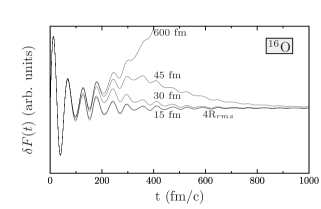
Figure 1: Evolution of the monopole moment in ${}^{16}\mbox{O}$ after a monopole boost with different values of the upper limit $R_{cut}$ in the integral of Eq. (3).

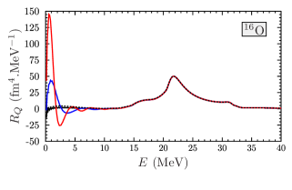
Figure 2: (Color online) Strength function of the GMR in ${}^{16}\mbox{O}$ computed from the time evolutions of the monopole moment $\delta{F}(t)$ with $R_{cut}=4R_{rms}$ (solid black line), 30 fm (blue line), and 45 fm (red line). The dashed black line has been obtained with $R_{cut}=4R_{rms}$ and a boost velocity $2\varepsilon$.

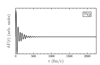
Figure 3: Evolution of the monopole moment in ${}^{16}\mbox{O}$ after a monopole boost in linear regime with $R_{cut}=4R_{rms}$ and with the SLy4 parametrization of the Skyrme EDF.

The evolution of $\delta{F}(t)$ over the maximum evolution time is shown in Fig. 3. A damped oscillation associated to the GMR is observed, with an average period $T_{GMR}\simeq 57.9$ fm/$c$ corresponding to an energy $E_{GMR}=2\pi\hbar/T_{GMR}$ $\simeq 21.4$ MeV. In a coherent state picture (see, e.g., sim01 ), the number of excited phonons is proportional to the square of the oscillation amplitude. The damping of the oscillation is then a signature for GMR decay. Here, the decay occurs by nucleon emission as $E_{GMR}$ is greater than the proton and neutron separation thresholds in ¹⁶O. The description of nucleon emission is possible if the continuum is properly accounted for. This is ensured, here, by the large size of the spherical mesh to prevent spurious effects coming from reflected flux on the edge of the box Rei06 .

The strength function associated to $\delta{F}(t)$ is plotted in Fig. 4 (black solid line). The main peak at $\sim{E}_{GMR}$ is surrounded by two shoulders at $\sim 17$ and $\sim 31$ MeV. In order to get a deeper insight into the microscopic origin of these structures, the spectral responses of the $\delta{F}_{lj}(t)$ [see Eq. (8)] following the same monopole boost are computed from Eq. (6) and plotted with colored lines in Fig. 4. We have checked numerically that the sum of these spectral functions is equal to the total strength function $R_{F}$, as expected. This decomposition shows that the low-energy shoulder and the main peak are mainly due to $p_{1/2}$ and $p_{3/2}$ orbitals, respectively. The structure of the high-energy shoulder is more complicated. It involves a constructive contribution of the $s_{1/2}$ orbitals. The dominant role of the $s_{1/2}$ neutron and proton contributions in the high-energy shoulder has already been noted using similar techniques but other EDF parametrizations Pac88 ; Ste10 . In addition, we see that the $p_{3/2}$ orbitals reduce the strength at $\sim 32$ MeV because $R_{F_{p3/2}}$ is negative in this region. Unlike strength functions ($\hat{Q}=\hat{F}$ case in section II.2), spectral responses of $\hat{Q}\neq\hat{F}$ are not necessarily strictly positive. In particular, it happens at frequencies $\omega\simeq\omega_{\nu}$ when $Re(\langle 0|\hat{Q}|\nu\rangle\langle\nu|\hat{F}|0\rangle)<0$. In this case, the $\omega$-component of $F(t)$ and $Q(t)$ oscillate with opposite phases. For the monopole response in ¹⁶O, this means that the contribution of the $p_{3/2}$ orbitals at $\sim 32$ MeV ”fight against” the mean-field which oscillates like $\delta{F}(t)$, generating a destructive contribution to the monopole strength function.

This microscopic decomposition of the strength function may vary with the parametrization of the Skyrme EDF. Indeed, the latter is usually fitted on global properties of nuclear systems, while the single-particle levels are not directly constrained. It is then worth comparing the above results with another parametrization of the Skyrme EDF. We chose the SGII parametrization which has been introduced to study compression modes in nuclei with a compression modulus $K_{\infty}\simeq 217$ MeV in infinite nuclear matter SGII . This value is slightly higher with SLy4, i.e., $K_{\infty}\simeq 230$ MeV. The results, shown in Fig. 5, are very similar to the calculations with the SLy4 parametrization.

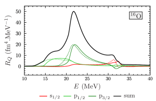
Figure 4: (Color online) Strength function of the GMR in ${}^{16}\mbox{O}$ (black solid line) computed from the time evolution of the monopole moment $\delta{F}(t)$ shown in Fig. 3 with the SLy4 parametrization of the Skyrme EDF. The spectral responses $R_{F_{lj}}$ associated to the single-particle quantum numbers $l$ and $j$ and labelled by their spectroscopic notation are plotted in colored solid (dashed) lines for neutrons (protons).

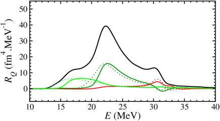
Figure 5: (Color online) Same as Fig. 4 with the SGII parametrization of the Skyrme EDF.

The monopole strength in ¹⁶O has been measured recently between 10 and 40 MeV energy excitation lui01 . The results are reported in Fig. 6 (black solid line) and compared to the TDHF monopole strength distribution (red dashed line). Approximatively half of the energy weighted sum rule has been found in this energy region. The rest of the strength distribution is expected to be found in low lying states at $E<10$ MeV, which could not be measured with the experimental setup, and at energies $E>40$ MeV. Note that the low-lying $0^{+}$ states, such as the one at $\sim 6$ MeV in ¹⁶O, can be reproduced only if 2p2h contributions are included in the model  gam10 . As a result, they are not seen in the present TDHF calculations.

The present calculations do not reproduce the peaks in the $10<E<15$ MeV region. In fact, the latter have been recently interpreted in terms of $\alpha$ cluster states (see thick solid blue line in Fig. 6) yam12 which are outside the space of 1p1h states. Note that monopole vibrations of $\alpha$ cluster configurations in light nuclei have also been recently investigated with Fermionic Molecular Dynamics (FMD) calculations fur10 .

The strength distribution of the GMR, as predicted by the present TDHF calculations, extends from $\sim 15$ to $33$ MeV. As shown in Fig. 6, the experimental strength in this region clearly exhibits three peaks at positions which could tentatively be associated to the $p_{1/2}$ ($E\sim 15-20$ MeV), $p_{3/2}$ ($E\sim 20-26$ MeV), and $s_{1/2}$ ($E\sim 28-33$ MeV) contributions of the TDHF response in Fig. 4. Similar three peak structures in the ¹⁶O GMR have been obtained in several microscopic calculations ma97 ; gam10 ; gam11 ; gam12 ; pap09 . The relative weight of the first peak is underestimated by the TDHF calculations. A possible explanation is that states with 2p2h contributions might be present, and even dominate, in this region of the spectrum.

It is also interesting to note that the width of these peaks (in particular the one in the $20-26$ MeV region) seems to be of the same order than the TDHF prediction. Assuming that the present TDHF calculations provide a good estimate of $\Gamma^{\uparrow}$ and $\Gamma^{L}$, this would imply that $\Gamma^{\downarrow}$ is only a correction to the total width of the GMR in ¹⁶O. Of course, $\Gamma^{\downarrow}$ could not be neglected in heavier nuclei such as tin isotopes where it account for about half of the total width tse09 .

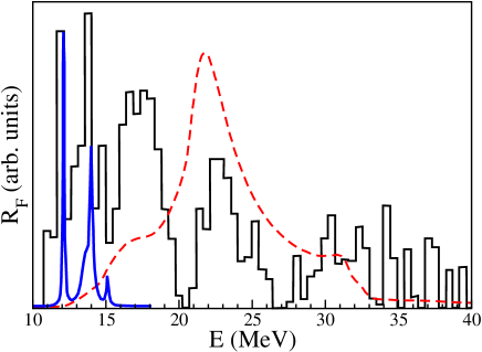
Figure 6: (Color online) Experimental monopole strength distribution in ${}^{16}\mbox{O}$ from Ref. lui01 (black solid line). The TDHF strength function is reported in dashed red line. The normalization is arbitrary. The thick solid blue line shows monopole strength expected from states with $\alpha$ clustering (From Ref. yam12 ).

The next step of our analysis is to study the decay properties of the GMR and to investigate their relationship with the previous microscopic decomposition. The spectra of emitted nucleons are computed at $T=2250$ fm/$c$ after the boost, e.g., when the monopole oscillation is fully damped (see Fig. 3). We use the method described in Sec. II.4. The proton and neutron spectra for each set of $l$ and $j$ are plotted in Fig. 7. We have checked numerically that, in the linear regime, these spectra are quadratic in the intensity of the boost $\epsilon$ Cho87 .

First we note that proton and neutron spectra have similar global features, as expected for light $N=Z$ nuclei, although the proton spectra are shifted by $\sim 3$ MeV due to the Coulomb repulsion. In addition, the Coulomb barrier, which is $B_{c}\simeq 1.7$ MeV in ¹⁶O, reduces strongly the emission of protons at energy $E<B_{c}$ due to the exponentially decreasing tunneling probability. We also note that there is no relevant emission of $s_{1/2}$ orbitals. In fact, the single-particle energy of the $1s_{1/2}$ orbitals, which are the only occupied $s_{1/2}$ single-particle states in the HF ground-sate of ¹⁶O, are $-32.4$ MeV for protons and $-36.2$ for neutrons (see table 1). As a result, the 1p1h states with a hole in a $1s_{1/2}$ orbital, and contributing to the GMR microscopic structure, are bound for neutrons and below $B_{c}$ for protons. Indeed, the different structures in the GMR spectrum (see Fig. 4) are located at energies below $\sim 33$ MeV, which is not sufficient to emit a $1s_{1/2}$ single-particle.

Table 1: Energies (in MeV) of the occupied single-particle states in the HF ground state of ¹⁶O with the SLy4 parametrization.

s.p. state	proton	neutron
$1s_{1/2}$	-32.4	-36.2
$1p_{3/2}$	-17.1	-20.6
$1p_{1/2}$	-11.2	-14.5

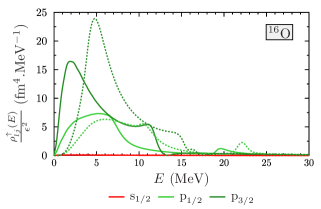
Figure 7: (Color online) Neutron (solid lines) and proton (dashed lines) direct-decay spectra of the GMR in ${}^{16}\mbox{O}$ for each set of single-particle quantum numbers $l$ and $j$, given in spectroscopic notation.

Let us now attempt to reconstruct the GMR strength function from the spectra of emitted nucleons shown in Fig. 7. In a pure harmonic picture, the GMR is a coherent sum of 1p1h states with a difference $\sim{E}_{GMR}$ between the particle and the hole energies. However, nucleons emitted by direct decay have only an energy $\sim$ to the one of a particle-state, which is obviously smaller than $E_{GMR}$ because the energy of the hole-state is negative. To approximately reconstruct the GMR strength function, it is then necessary to shift the energy of the emitted nucleons by the energy of their associated hole-state, that is, the energy of the initially occupied single-particle state. The latter are given in table 1 for ¹⁶O at the HF level. The “shifted” spectra of emitted nucleons for each set of $l$ and $j$, noted $\rho^{\uparrow(s)}_{lj}$, obtained from this procedure, are plotted in Fig. 8-b, together with their sum. It is striking to see that, not only the shape, but also the magnitude of the latter is very similar to the strength function shown in Fig. 4 and recalled in Fig. 8-a, although the two spectra have been obtained from totally different quantities, i.e., the spectra of emitted nucleons and the time evolution of the monopole moment. A theoretical justification of these similarities is outlined in section II.4.2.

Similarly to the microscopic decomposition of the strength function obtained from the time evolution of the monopole moment (see Fig. 4), we see in Fig. 8-b that the low energy shoulder and the main peak are associated to $p_{1/2}$ and $p_{3/2}$ orbitals, respectively. Again, the situation for the high energy shoulder is more complicated. Although it is mainly due to $s_{1/2}$ orbitals in the monopole response (see Fig. 4), it is in fact associated to the emission of $p$-orbitals in Fig. 8-b. As discussed before, this is because the energy of the GMR is not sufficient to promote a $1s_{1/2}$ single-particle to the continuum. However, the RPA residual interaction couples the responses associated to the different single-particle quantum numbers to produce a collective monopole vibration. As a result, the vibration of $s$-orbitals can be coupled to $p$-unbound-states contributing to the direct decay. Such coupling might be the reason for the complex competition between constructive and destructive contributions in the high-energy shoulder observed in Fig. 4.

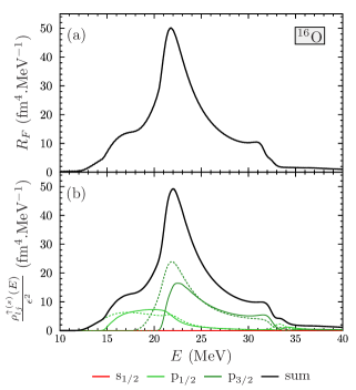
Figure 8: (Color online) (a) Strength function of the GMR in ¹⁶O obtained from the time evolution of the monopole moment. (b) Spectra of emitted neutrons (colored solid lines) and protons (colored dashed lines) ”shifted” by the energy of the initially occupied single-particle state (see text). Their sum is shown in black solid line.

III.2 $A=100$ and $132$ tin isotopes

Similar analyses have been performed for the GMR in ^100,132Sn nuclei. The strength functions obtained from the time evolution of the monopole moment are plotted with black solid lines in the upper panels of Fig. 9 and 10. The reconstructed GMR strength, obtained from the emission spectra are plotted with black solid lines in the lower panels. As in the ¹⁶O case, the agreement between the two methods is excellent.

The gross feature of the strength is similar for the two isotopes, with a single peak centered at $E_{GMR}=17.2$ MeV for ${}^{100}\mbox{Sn}$ and $15.8$ MeV for ${}^{132}\mbox{Sn}$ (see table 2), although their widths vary more importantly. It is striking, however, that the decompositions in terms of single-particle quantum numbers exhibit some important differences between the two techniques. Although both proton and neutron single-particle orbitals participate to the vibration (see upper panels in Fig. 9 and 10), the decay only occurs by neutron emission for ${}^{132}\mbox{Sn}$, whereas ${}^{100}\mbox{Sn}$ decays through proton emission only. This can be understood by the fact that the proton (neutron) separation energy increases (decreases) with the number of neutrons. These quantities are given in table 2, together with the Coulomb barrier for protons and the position of the peak energy associated to the GMR energy. Indeed, the binding energy of neutrons in ¹⁰⁰Sn is of the order of $E_{GMR}$ and proton emission is favored, while the combined effects of an increasing $S_{p}$ and the Coulomb barrier $B_{c}$ prevent proton emission in ${}^{132}\mbox{Sn}$.

Table 2: Neutron and proton separation energies and Coulomb barriers in Sn isotopes. The GMR energy corresponds to the position of the peak in the strength function. All energies are in MeV.

	$S_{p}$	$B_{c}$	$S_{p}+B_{c}$	$S_{n}$	$E_{GMR}$
100Sn	3.1	8.1	11.4	16.9	17.2
132Sn	15.6	7.4	23.0	7.7	15.8

As in the case of the high-energy shoulder in the ¹⁶O spectra of figures 4 and 8, the difference in the microscopic decomposition of the GMR strength with the two techniques is a signature of the RPA residual interaction which couples the bound particle-hole states to the unbound ones, allowing their decay. In particular, the vibration of the protons (neutrons) in ¹³²Sn (¹⁰⁰Sn) decays via neutron (proton) emission thanks to the collective vibration of both proton and neutron mean-fields.

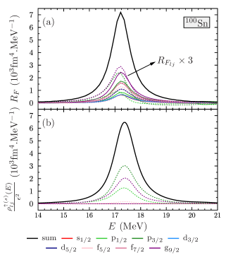
Figure 9: (Color online) (a) Strength function $R_{F}$ (black solid lines) of ${}^{100}\mbox{Sn}$. Its single-particle decomposition, multiplied by a factor of three ($R_{F_{lj}}\times 3$), is represented with colored solid (dashed) lines for neutrons (protons). (b) Spectra of emitted particles ”shifted” from their single-particle energies are plotted in colored solid (dashed) lines for neutrons (protons). Their sum appears in black.

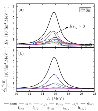
Figure 10: (Color online) Same as Fig. 9 for ${}^{132}\mbox{Sn}$.

IV Conclusions

Using a simple single-particle decomposition, the microscopic structure and (direct) decay of the GMR in some spherical nuclei has been studied in the harmonic picture using TDHF calculations. The GMR strength is usually obtained, in TDHF, using the Fourier analysis of the real-time small amplitude monopole response. We showed that, assuming that 2p2h and higher order configurations do not contribute significantly to the strength function, it can be also approximately reconstructed by shifting the energy spectra of emitted nucleons by their corresponding initial hole single-particle energy.

On this ground, we studied the microscopic structure of the GMR strengths obtained by these two techniques (standard real-time response and reconstruction from emitted nucleons), by decomposing it onto the single-particle quantum numbers $l$ and $j$. Although both techniques lead to almost identical monopole strengths, their microscopic structure may be very different. This is understood by the fact that, although GMR energies are usually above the nucleon emission thresholds, only part of the particle-hole states lie in the continuum. Those which are bound are coupled to unbound states via the RPA residual interaction which is responsible for the collectivity of the vibration. This is illustrated, e.g., in monopole spectra of neutron-rich tin isotopes: although both protons and neutrons contribute to the monopole vibration, only neutrons can be emitted because protons are more bound and have to overcome the Coulomb barrier.

A major improvement of the method would be to include two-body correlations, like pairing interaction and collision terms. Pairing correlations are expected to affect particle decay as compared to the independent particle picture sca12 , in particular by enhancing the direct two-proton decay mar12 . The collision term is known to be responsible for the additional spreading width of giant resonances as well as a fragmentation of their strength function Lac04 . They are also expected to modify the structure of the spectra of emitted nucleons by coupling 1p1h states to 2p2h. A first step would be to use the Extended-TDHF Won78 ; Ayi80 ; Lac99 or the time-dependent Density-Matrix Wan85 ; Toh01 ; Ass09 formalisms. Because of computational limitations, spherical symmetry (and thus, only monopole vibrations) might be first considered. Realistic spectra of emitted particles could then be computed and compared to experimental data. However, the reconstruction of the strength functions from these spectra will be more complicated as the simple technique introduced here, i.e., introducing a shift of the single particle hole energy, is valid only for 1p1h contributions. Finally, one could analyze the hole structure of the remaining nucleus as well, using, e.g., similar techniques as in Ref. sim10 ; sim11 to determine the particle number distributions for different $l$ and $j$ quantum numbers.

We thank T. Lesinski for providing the routine for computation of Bessel functions. We are also grateful for comments and discussions with Ph. Chomaz and D. Lacroix at the early stage of this work. Part of the calculations have been performed at the NCI National Facility in Canberra, Australia, which is supported by the Australian Commonwealth Government. Partial support from ARC Discovery grants DP0879679 and DP110102879, as well as ARC Future Fellowship FT120100760 is acknowledged.

References

- (1) A. Bohr and B. Mottelson, Nuclear Structure, (2 vol., W.A. Benjamin, Inc., 1975).
- (2) M. N. Harakeh and A. van der Woude, Giant Resonances: Fundamental High-Frequency Modes of Nuclear Excitation (Oxford University Press, 2001).
- (3) D. Pines, P. Nozières, The Theory of Quantum Liquids (Benjamin, New York, 1966).
- (4) D. Bohm and D. Pines, Phys. Rev. 92, 609 (1953).
- (5) M. L’Huillier and Nguyen Van Giai, Phys. Rev. C 39, 2022 (1989).
- (6) D. S. Oakley, J. R. Shepard, N. Auerbach, Phys. Rev. C 45, 2254 (1992).
- (7) D. Vretenar, G. A. Lalazissis, R. Behnsch, W. Poschl, and P. Ring, Nucl. Phys. A 621, 853 (1997).
- (8) P. Ring and P. Schuck, The Nuclear Many-Body Problem, (Springer Verlag, 1980).
- (9) C. Golabek and C. Simenel, Phys. Rev. Lett. 103, 042701 (2009).
- (10) D. J. Kedziora and C. Simenel, Phys. Rev. C 81, 044613 (2010).
- (11) A. S. Umar and V. E. Oberacker, Phys. Rev. C 71, 034314 (2005).
- (12) J. A. Maruhn, P.-G. Reinhard, P. D. Stevenson, J. R. Stone and M. R. Strayer, Phys. Rev. C 71, 064328 (2005).
- (13) T. Nakatsukasa and K. Yabana, Phys. Rev. C 71, 024301 (2005).
- (14) S. Fracasso, E. B. Suckling, and P. D. Stevenson Phys. Rev. C 86, 044303 (2012).
- (15) C. Simenel, Eur. Phys. J. A 48, 152 (2012).
- (16) J.-P. Blaizot and G. Ripka, Quantum Theory of Finite Systems, (MIT Press, 1986).
- (17) J. Engel, M. Bender, J. Dobaczewski, W. Nazarewicz, R. Surman, Phys. Rev. C 60, 014302 (1999).
- (18) E. Khan, N. Sandulescu, M. Grasso and N. V. Giai, Phys. Rev. C 66, 024309 (2002).
- (19) E. Khan, N. Sandulescu, N. Van Giai, M. Grasso, Phys. Rev. C 69, 014314 (2004).
- (20) S. Fracasso, G. Colò, Phys. Rev. C 72, 064310 (2005).
- (21) S. Péru, H. Goutte, Phys. Rev. C 77, 044313 (2008).
- (22) K. Yoshida and T. Nakatsukasa, Phys. Rev. C 83, 021304(R) (2011).
- (23) B. Avez, C. Simenel and P. Chomaz, Phys. Rev. C 78, 044318 (2008).
- (24) S. Ebata, T. Nakatsukasa, T. Inakura, K. Yoshida, Y. Hashimoto and K. Yabana, Phys. Rev. C 82, 034306 (2010).
- (25) I. Stetcu, A. Bulgac, P. Magierski, K. J. Roche, Phys.Rev. C 84, 051309 (2011).
- (26) Y. Aschimoto, Eur. Phys. J. A 48, 55 (2012).
- (27) P. F. Bortignon and R. A. Broglia, Nucl. Phys. A 371, 405 (1981).
- (28) S. Kamerdzhiev, J. Speth, and G. Tertychny, Phys. Rep. 393, 1 (2004).
- (29) V. Tselyaev, J. Speth, S. Krewald, E. Litvinova, S. Kamerdzhiev, N. Lyutorovich, A. Avdeenkov, and F. Grümmer, Phys. Rev. C 79, 034309 (2009).
- (30) D. Lacroix, S. Ayik and P. Chomaz, Prog. Part. Nucl. Phys. 52, 497 (2004).
- (31) M.Tohyama, Phys. Rev. C 64, 067304 (2001).
- (32) S. Drozdz, S. Nishizaki, J. Speth, and J. Wambach, Phys. Rep. 197, 1 (1990).
- (33) D. Gambacurta, M. Grasso, and F. Catara, Phys. Rev. C 81, 054312 (2010).
- (34) D. Gambacurta, M. Grasso, and F. Catara, J. Phys. G 38, 035103 (2011).
- (35) D. Gambacurta, M. Grasso, V. De Vonno, G. Co’, and F. Catara, Phys. Rev. C 86, 021304(R) (2012).
- (36) P. Papakonstantinou and R. Roth, Phys. Lett. B 671, 356 (2009).
- (37) C. Simenel and P. Chomaz, Phys. Rev. C 68, 024302 (2003).
- (38) C. Simenel and P. Chomaz, Phys. Rev. C 80, 064309 (2009).
- (39) S. Strauch, P. von Neumann-Cosel, C. Rangacharyulu, A. Richter, G. Schrieder, K. Schweda and J. Wambach, Phys. Rev. Lett. 85, 2913 (2000).
- (40) R. G. T. Zegers et al., Phys. Rev. Lett. 90, 202501 (2003).
- (41) M. Hunyadi et al., Phys. Rev. C 75, 014606 (2007).
- (42) S. Krewald, J. Birkholz, A. Faessler, J. Speth, Phys. Rev. Lett. 33, 1386 (1974).
- (43) K. Liu, N.V. Giai, Phys. Lett. B 65, 23 (1976).
- (44) S. Kamerdzhiev, R.J. Liotta, E. Litvinova, V. Tselyaev, Phys. Rev. C 58, 172 (1998).
- (45) M. Matsuo, Nucl. Phys. A 696, 371 (2001).
- (46) K. Hagino, H. Sagawa, Nucl. Phys. A 695, 82 (2001).
- (47) P. Chomaz,N. V. Giai and S. Stringari, Phys. Lett. B 189, ) 375 (1987.
- (48) J. M. Pacheco, E. Maglione and R. A. Broglia, Phys. Rev. C 37, 2257 (1988).
- (49) P. A. M. Dirac, Proc. Cambridge Philos. Soc. 26, 376 (1930).
- (50) T. Skyrme, Phil. Mag. 1, 1043 (1956).
- (51) Y.-W. Lui, H. L. Clark, and D. H. Youngblood, Phys. Rev. C 64, 064308 (2001).
- (52) R. Balian and M. Vénéroni, Phys. Rev. Lett. 47 1353 , (1981).
- (53) J. Blocki and H. Flocard, Phys. Lett. B 85, 163 (1979).
- (54) D. Almehed and P. D. Stevenson, J. Phys. G 31, S1819 (2005).
- (55) T. Nakatsukasa and K. Yabana, Nucl. Phys. A 788, 349 (2007).
- (56) P. Stevenson, D. Almehed, P.-G. Reinhard and J. Maruhn, Nucl. Phys. A 788, 343 (2007).
- (57) P. D. Stevenson and S. Fracasso, J. Phys. G 37, 064030 (2010).
- (58) P. G. Reinhard, L. Guo and J. A. Maruhn, Eur. Phys. J. A 32, 19 (2007).
- (59) D. Varshalovich, A. Moskalev and V. Khersonskii, Quantum Theory of Angular Momentum (World Scientific, 1988).
- (60) D. J. Thouless, Nucl. Phys. 21, 225 (1960).
- (61) E. Chabanat, P. Bonche, P. Haensel, J. Meyer and R. Schaeffer, Nucl. Phys. A 635, 231 (1998).
- (62) P.-G. Reinhard, P. D. Stevenson, D. Almehed, J. A. Maruhn and M. R. Strayer, Phys. Rev. E 73, 036709 (2006).
- (63) S. Stringari and D. Vautherin, Phys. Lett. B 88, 1 (1979).
- (64) K. Bennaceur and J. Dobaczewski, Comp. Phys. Comm. 168, 96 (2005).
- (65) C. Simenel, P. Chomaz and G. de France, Phys. Rev. Lett. 86, 2971 (2001).
- (66) N.V. Giai and H. Sagawa, Nucl. Phys. A 371, 1 (1981).
- (67) T. Yamada, Y. Funaki, T. Myo, H. Horiuchi, K. Ikeda, G. Röpke, P. Schuck, and A. Tohsaki, Phys. Rev. C 85, 034315 (2012).
- (68) T. Furuta, K. H. O. Hasnaoui, F. Gulminelli, C. Leclercq, and A. Ono, Phys. Rev. C 82, 034307 (2010).
- (69) Z. Ma, N. Van Giai, and H. Toki, Phys. Rev. C 55, 2385 (1997).
- (70) G. Scamps, D. Lacroix, G. F. Bertsch, and K. Washiyama, Phys. Rev. C 85, 034328 (2012).
- (71) T. Maruyama, T. Oishi, K. Hagino, and H. Sagawa, Phys. Rev. C 86, 044301 (2012).
- (72) C.-Y. Wong and H. H. K. Tang, Phys. Rev. Lett. 40, 1070 (1978).
- (73) S. Ayik, Z. Phys. A 298, 83 (1980).
- (74) D. Lacroix, P. Chomaz and S. Ayik, Nucl. Phys. A 651, 369 (1999).
- (75) S. Wang and W. Cassing, Ann. Phys. (N.Y.) 159, 328 (1985).
- (76) M. Assié and D. Lacroix, Phys. Rev. Lett. 102, 202501 (2009).
- (77) C. Simenel, Phys. Rev. Lett. 105, 192701 (2010).
- (78) C. Simenel, Phys. Rev. Lett. 106, 112502 (2011).