Effective medium theory of binary thermoelectrics.

Abstract

The transport coefficients of disordered media are analyzed using direct numerical simulation and effective medium theory. The results indicate a range of materials parameters for which disorder leads to an enhanced power factor. This increase in power factor is generally not accompanied by an increase in the figure of merit $ZT$, however. It is also found that the effective electrical conductivity and electronic contribution to the thermal conductivity are not generally proportional to each other in the presence of disorder.

I introduction

There has been considerable recent interest in utilizing nanostructure and inhomogeneity to enhance thermoelectric performance. Nanostructure has been predicted to reduce phonon thermal conductivity without reducing electrical conductivity venk , enhance the power factor via quantum confinement harman , and provide strongly energy-dependent electron scattering leonard ; moyzhes ; martin - beneficial features for thermoelectrics. One type of nanostructure consists of the inclusion of metallic structures in a thermoelectric (i.e semiconductor) framework. These types of nanostructured materials can exhibit two unusual properties: unexpectedly high Seeback coefficient heremans , and anomalous magnetoresistance xu . The anomalous magnetoresistive properties can be understood as a consequence of disordered transport in a random resistor network model littlewood .

Motivated by these models of magnetoresistance, I revisit similar models of thermoelectric properties cohen to see if the same mechanism can explain both phenomena. The work presented here extends previous studies in two ways: 1. The electrical conductivity and Seeback coefficient of the constituent materials are varied independently. It’s found that in certain parameter regimes the thermoelectric power factor of the composite medium is enhanced relative to that of the constituent materials. 2. The electron and phonon contributions to the total thermal conductivity are calculated separately. Although the constituent materials are assumed to be obey the Weidemann-Franz law (W-F), the composite medium does not. Finally, in accordance with previous studies levy , the figure of merit $ZT$ of the composite medium is found to be smaller than that of the high-$ZT$ constituent material. These conclusions are illustrated with numerical results and analytic expressions derived within effective medium theory (EMT).

II Model description

The starting point is the linear response description of transport for the electrical current $j$ and thermal current $j_{Q}$:

$$j = -\sigma\left({\bf r}\right)\nabla V+L^{12}\left({\bf r}\right)\nabla T~{},$$

$$j_{Q} = -\left(\kappa_{e}\left({\bf r}\right)+\kappa_{\gamma}\left({\bf r}\right)\right)\nabla T+L^{12}\left({\bf r}\right)T\nabla V~{},$$ (1)

where $\sigma\left({\bf r}\right)$ is the local electrical conductivity, $\kappa_{e}^{\prime}~{}\left(\kappa_{\gamma}^{\prime}\right)$ is the electron (phonon) contribution to the total local thermal conductivity $\kappa\left({\bf r}\right)$ ($\kappa\left({\bf r}\right)=\kappa_{e}^{\prime}\left({\bf r}\right)+\kappa_{\gamma}^{\prime}\left({\bf r}\right)$) (all thermal conductivities evaluated for zero electric field), $V$ is the electrostatic potential, and $T$ is the temperature. The local Seeback coefficient $S\left({\bf r}\right)$ is related to $\sigma\left({\bf r}\right)$ and $L^{12}\left({\bf r}\right)$ by: $L^{12}\left({\bf r}\right)=S\left({\bf r}\right)\sigma\left({\bf r}\right)$. I assume that $\sigma\left({\bf r}\right)$ and $\kappa_{e}\left({\bf r}\right)$ obey the W-F law: $\kappa_{e}\left({\bf r}\right)=\sigma\left({\bf r}\right)L_{0}T$, where $L_{0}$ is the Lorenz number. As shown in Ref. (cohen, ), the effective medium electrical conductivity $\bar{\sigma}$, total thermal conductivity $\bar{\kappa}$, and $\bar{L}^{12}$ satisfy:

$$\left\langle\frac{\sigma\left({\bf r}\right)-\bar{\sigma}}{\sigma\left({\bf r}\right)+2\bar{\sigma}}\right\rangle=0~{}; \left\langle\frac{\kappa\left({\bf r}\right)-\bar{\kappa}}{\kappa\left({\bf r}\right)+2\bar{\kappa}}\right\rangle=0~{},$$ (2)

$$\bar{L}^{12}= 3\bar{\sigma}\bar{\kappa}\left\langle\frac{L^{12}\left({\bf r}\right)}{\left(\kappa\left({\bf r}\right)+2\bar{\kappa}\right)\left(\sigma\left({\bf r}\right)+2\bar{\sigma}\right)}\right\rangle\times$$ (3)

$$\left(\left\langle\frac{\sigma\left({\bf r}\right)\bar{\kappa}+\bar{\sigma}\kappa\left({\bf r}\right)+2\bar{\sigma}\bar{\kappa}-\sigma\left({\bf r}\right)\kappa\left({\bf r}\right)}{\left(\kappa\left({\bf r}\right)+2\bar{\kappa}\right)\left(\sigma\left({\bf r}\right)+2\bar{\sigma}\right)}\right\rangle\right)^{-1}.$$

The brackets indicate an average over disorder configurations. In addition, the electron and phonon parts of the thermal conductivity of the effective medium, $\bar{\kappa}_{e}$ and $\bar{\kappa}_{\gamma}$, satisfy:

$$\left\langle\frac{\kappa_{e,\gamma}\left({\bf r}\right)-\bar{\kappa}_{e,\gamma}}{\kappa\left({\bf r}\right)+2\bar{\kappa}}\right\rangle = 0~{},$$ (4)

Two-component materials are considered here, so that local material parameters may assume one of two possible values. I further suppose that $\sigma_{1}\ll\sigma_{2}$, and $\kappa_{\gamma 1,2}\ll\kappa_{e2}$.

The figure of merit $ZT$ can be expressed with the Onsager number $N$ (note that $N$ is constrained thermodynamically to be less than 1 davidson ; mahan ).

$$N = \frac{\left(\bar{L}^{12}\right)^{2}T}{\bar{\sigma}\bar{\kappa}_{e}}~{},$$ (5)

$$ZT = \frac{N}{1-N+\left(\frac{\bar{\kappa}_{\gamma}}{\bar{\kappa}_{e}}\right)}~{}.$$ (6)

In addition to the analysis of EMT, Eq. (1) and the continuity equations for heat and charge ($\nabla\cdot j=0$, $\nabla\cdot j_{Q}=0$ footnote ) are solved directly for an ensemble of randomly disordered configurations in 3-d (correlated disorder does not change the results appreciably). The system is discretized into $30^{3}$ sites, and the ensemble size is chosen such that the statistical error of the effective transport parameters is converged (this typically requires about 30 configurations). The error bars on the plots of numerical results indicate the statistical uncertainty (one standard deviation).

III Results

Power factor - Figs. 1(a), 1(b), and 1(c) show $\bar{\sigma},~{}\bar{L}^{12}$, and the power factor $\bar{S}^{2}\bar{\sigma}$, respectively, as a function of concentration of material 1 (denoted by $c$). For this calculation $L^{12}_{1}=L^{12}_{2}$. At the percolation threshold ($c=2/3$), $\bar{\sigma}$ shows a well-known kink kirkpatrick , while $\bar{L}^{12}$ is maximized. The origin of this enhancement in $\bar{L}^{12}$ is discussed in the next section. The enhancement in $\bar{L}^{12}$ leads to a peak in the the power factor $\bar{S}^{2}\bar{\sigma}$ near the percolation threshold. The figure shows good agreement between EMT and numerical results, indicating the EMT captures the essential physics of the power factor enhancement. Fig. 1(d) shows the Seeback coefficient versus concentration when the correct effective medium $L^{12}$ value is used to calculate $S$, and when it is assumed that $L^{12}$ of the composite medium is the same as that of the constituent materials.

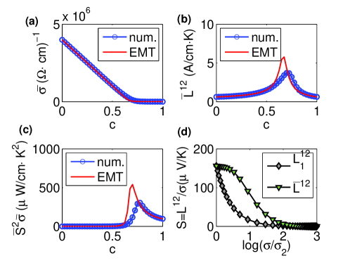
Figure 1: (a), (b), (c) show the effective conductivity, $L^{12}$, and power factor as a function of disorder concentration. (d) shows the Seeback coefficient $S=P/\sigma$ as a function of conductivity (note the log scale of conductivity), using $L^{12}=\bar{L}^{12},~{}L^{12}=L^{12}_{1}$. Model parameters are: $\sigma_{1}=4\times 10^{5}~{}{\rm\frac{1}{\Omega\cdot m}}$, $f_{s}=10^{3}$, $\kappa_{1\gamma}=3~{}{\rm\frac{W}{m\cdot K}}$, $\kappa_{2\gamma}=1~{}{\rm\frac{W}{m\cdot K}}$, $L^{12}_{1}=L^{12}_{2}=\sqrt{L_{0}}\sigma_{1}=62.5~{}{\rm\frac{A}{m\cdot K}}$.

To explain the peak in power factor, I solve Eqs. (2-3) at the percolation transition ($c=2/3$), and expand the solution in the small parameters:

$$f_{s}=\frac{\sigma_{1}}{\sigma_{2}}; f_{k}=\frac{\kappa_{1}}{\kappa_{2}}.$$ (7)

Keeping only leading order terms leads to:

$$\bar{\sigma} = \sqrt{\frac{\sigma_{1}\sigma_{2}}{2}}=\sigma_{1}\sqrt{\frac{1}{2f_{s}}}+\ldots$$ (8)

$$\bar{L}^{12} = L^{12}_{1}\left(\sqrt{2f_{k}}+\sqrt{2f_{s}}\right)^{-1}+\ldots$$ (9)

Eq. (9) is valid when $L^{12}_{2}$ is not significantly (e.g more than 100 times) greater than $L^{12}_{1}$. Eqs. (8) and(9) show that both $\bar{\sigma}$ and $\bar{L}^{12}$ diverge as $f_{s}^{-1/2}$ at the percolation transition. This implies that the power factor ($\left(\bar{L}^{12}\right)^{2}/\bar{\sigma}$) also diverges as $f_{s}^{-1/2}$ at this point, while the Seeback coefficient ($\bar{L}^{12}/\bar{\sigma}$) remains bounded within EMT. The divergence of transport parameters at the percolation transition signals a failure of effective medium theory in the limit $f_{s}\rightarrow 0$. However the numerics indicate that EMT is sufficient for realistic parameters, and can illustrate the key points in this work.

To develop a simple picture for how inhomogeneity leads to an enhancement in $L^{12}$, I consider Eq. (1) for two dissimilar materials placed in series (see Fig. (2)), where $\sigma_{1}\ll\sigma_{2},~{}\kappa_{1}\ll\kappa_{2},$ and $L^{12}_{1}=L^{12}_{2}$. $L^{12}$ of the composite system is given by $\frac{j}{\Delta T}|_{\Delta V=0}$. The large thermal resistance of material 1 implies the temperature drop occurs mostly between sites 1 and 2. This drives a large thermoelectric charge current between sites 1 and 2, which in turn induces a voltage at site 2. This voltage drives an Ohmic charge current between sites 2 and 3. This Ohmic current, derived from the inhomogeneous voltage, is the source of enhanced charge current (and therefore enhanced $L^{12}$) of the composite system. The same scenario occurs in 3-dimensional disordered networks of materials (under the same parameter region described above), so that when the system is maximally disordered at the percolation transition, $L^{12}$ shows the maximum enhancement.

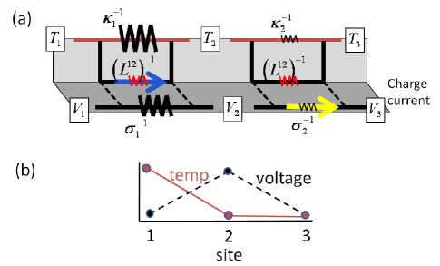
Figure 2: Cartoon indicating the underlying mechanism for the enhancement of $L^{12}$ for an inhomogeneous systems consisting of 2 resistors. (a) shows the predominant paths for charge current, (b) shows the voltage and temperature profiles for an applied temperature difference.

Thermal conductivity - Next I consider the electronic and phonon contributions to the thermal conductivity of the disordered material. Let $\kappa_{\gamma 1}>\kappa_{\gamma 2}$; this describes a system in which one material has good electronic thermoelectric properties (i.e. a large Onsager number), but a detrimentally large $\kappa_{\gamma}$, while the other material has a low Onsager number and a small $\kappa_{\gamma}$. I assume that both $\frac{\kappa_{\gamma 1}}{\kappa_{e2}}$ and $\frac{\kappa_{\gamma 2}}{\kappa_{e2}}$ are small (of the same order as $\frac{\kappa_{e1}}{\kappa_{e2}}$). Fig. (3a) shows $\kappa_{e}$ and $\kappa_{\gamma}$ as a function of concentration. There is good agreement between numerical results and EMT. Fig. (3b) shows that near the percolation threshold, the electronic contribution to the thermal conductivity is not related to the electrical conductivity via the W-F law. At the percolation threshold, the expressions for the total thermal conductivity $\kappa$ and its partition into electronic and phonon parts $\kappa_{e},\kappa_{\gamma}$ are given as (to linear order in $f_{k},f_{s}$):

$$\bar{\kappa} = \kappa_{2}\left[\sqrt{\frac{f_{k}}{2}}+\frac{f_{k}}{4}+\ldots\right]$$ (10)

$$\bar{\kappa}_{e} = \kappa_{2,e}\left[\sqrt{\frac{f_{k}}{2}}+\left(f_{s}-\frac{3f_{k}}{4}\right)+\ldots\right]$$ (11)

$$\bar{\kappa}_{\gamma} = \kappa_{1,\gamma}+\ldots$$ (12)

The ratio $\sigma/\kappa_{e}$ is easily expressed in terms of $r=f_{k}/f_{s}$:

$$\frac{\bar{\sigma}}{\bar{\kappa}_{e}}=L_{0}T\frac{1}{\sqrt{r}}~{}.$$ (13)

This indicates that in inhomogeneous materials, inferring $\kappa_{e}$ from $\sigma$ may not always be appropriate near the percolation transition. This is because the effective $\kappa_{e}$ is a convolution of the intrinsic material properties and the geometry of the system: The parallel conduction of heat current through both electron and phonon channels (in contrast to the charge current) results in different conducting paths for $j_{Q}$ and $j$, and differences in the spatial structure of temperature and potential fields. As a result, the electronic part of $j_{Q}$ in the inhomogeneous system is not exactly correlated with $j$.

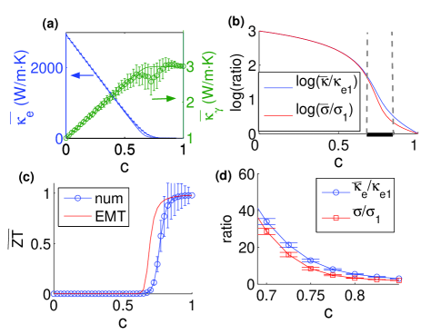
Figure 3: (a) shows the electron and phonon contributions to the total thermal conductivity as a function of concentration of material 1 (this concentration is denoted by $c$). Solid lines are EMT result, symbols are numerical results. (b) shows the electrical conductivity and electron contribution to thermal conductivity (scaled by the value of material 1 versus concentration (note log scale). Vertical dashed lines indicate region that is plotted in (d). (c) shows the figure of merit $ZT$ as a function of concentration. It generally decreases from the high material value of $ZT=1$. (d) is a zoom-in of (b) near percolation (on a linear scale), showing the deviation from the W-F law of the composite medium

Figure of merit - The electronic and phonon contributions to $ZT$ can now be assembled. At percolation, the Onsager number and ratio of electronic to phonon thermal conductivity are:

$$N = N_{1}\frac{1}{\sqrt{r}\left(1+r+2\sqrt{r}\right)}$$ (14)

$$\frac{\bar{\kappa}_{\gamma}}{\bar{\kappa}_{e}} = \sqrt{\frac{2}{f_{k}}}\left(\frac{\kappa_{\gamma,1}}{\kappa_{e,2}}\right)$$ (15)

Plugging the above into Eq. (6) shows that $ZT$ of the composite medium is always smaller than that of the high-$ZT$ material constituent. Fig. (3c) shows $ZT$ as a function of concentration. It is seen that under the favorable parameter set considered here, the high $ZT$ value is maintained for a substantial amount of low $ZT$ material doping. Generally $ZT$ shows a decrease by percolation, and rises rapidly to the high value just above this threshold.

I note that this model ignores interface scattering contributions to $\sigma,\kappa$, and $L^{12}$. If these contributions lower $\kappa$ and $\sigma$ more drastically than $L^{12}$, it would imply an overall enhancement in $ZT$ leonard . A more complete theory requires a combination of bulk modeling as presented here, combined with more microscopic modeling of materials interfaces. Nevertheless the model demonstrates that disorder in the diffusive regime can explain the enhancement in power factor, and can alter the relationship between electrical and thermal conductivity of electrons. These are both important considerations in the interpretation of experimental results, and in assessing the viability of materials for improved thermoelectric efficiencies.

I gratefully acknowledge very helpful conversations with Fred Sharifi, who introduced me to this problem.

References

- (1) R. Venkatasubramanian, E. Siivola, T. Colpitts, and B. O Quinn, Nature 413, 597 (2001).
- (2) T. C. Harman, P. J. Taylor, M. P. Walsh, and B. E. LaForge, Science 29, 2229 (2002).
- (3) S. V. Faleev and F. Léonard, Phys. Rev. B 77, 214304 (2008).
- (4) Moyzhes and V. Nemchinsky, Appl. Phys. Lett. 73, 1895 (1998).
- (5) J. Martin, L. Wang, L. Chen, and G. S. Nolas, Phys. Rev. B 79, 115311 (2009).
- (6) J. P. Heremans, C. M. Thrush, and D. T. Morelli, J. App. Phys. 98, 063703 (2005).
- (7) R. Xu , Nature 390, 57 (1997).
- (8) M. M. Parish and P. B. Littlewood, Nature 426, 162 (2003).
- (9) I. Webman, J. Jortner, and M. H. Cohen, Phys. Rev. B 16, 2959 (1977).
- (10) D. J. Bergman and 0. Levy, J. App. Phys. 70, 6821 (1991).
- (11) H. Littman and B. Davidson, J. App. Phys. 32, 217 (1961).
- (12) G. D. Mahan and J.O. Sofo, Proc. Natl. Acad. Sci. USA 93, 7436 (1996).
- (13) The equation of continuity for heat current is generally . In linear response the right-hand-side of this equation can generally be ignored. The full nonlinear version with heating was solved in the numerical calculation, and was found to agree with the results when heating is neglected.
- (14) S. Kirkpatrick, Phys. Rev. Lett. 27, 1722 (1971).
- (15) N. Mori, H. Okana, and A. Furuya, Phys. Stat. Sol. (a) 203, 2828 (2006).