Kinetic Monte Carlo Simulations of a Model for Heat-assisted Magnetization Reversal in Ultrathin Films

Abstract

To develop practically useful systems for ultra-high-density information recording with densities above terabits/cm², it is necessary to simultaneously achieve high thermal stability at room temperature and high recording rates. One method that has been proposed to reach this goal is heat-assisted magnetization reversal (HAMR). In this method, the magnetic orientation is assigned to a high-coercivity material by temporarily reducing the coercivity during the writing process through localized heating. Here we present kinetic Monte Carlo simulations of a model of HAMR for ultrathin films, in which the temperature in the central part of the film is momentarily increased above the critical temperature, for example by a laser pulse. We observe that the speed-up achieved by this method, relative to the switching time at a constant, subcritical temperature, is optimal for an intermediate strength of the writing field. This effect is explained using the theory of nucleation-induced magnetization switching in finite systems. Our results should be particularly relevant to recording media with strong perpendicular anisotropy, such as ultrathin Co/Pt or Co/Pd multilayers.

I Introduction

One of the most important factors supporting progress in the miniaturization of computers and other electronic devices is the continued exponential increase in the density of data storage.McDaniel (2005) Currently, designs are being considered for magnetic recording devices that have areal data densities of the order of terabits/cm² – several orders of magnitude more than only a decade ago. At such densities, the size of the recording bit approaches the superparamagnetic limit, where thermal fluctuations seriously degrade the stability of the magnetization.Bean and Livingston (1959); Richards et al. (1995) However, current industry standards demand that bits should retain 95% of their magnetization over a period of ten years.McDaniel (2005) Furthermore, subnanosecond magnetization-switching times are required to achieve acceptable read/write rates.

One suggested method to fulfill these requirements is to use ultrathin, perpendicularly magnetized films of very high-coercivity materials, such as FePt (coercive field about 50 kOe), or single-particle bits that are expected to have even higher coercivities.McDaniel (2005) However, such high coercive fields at room temperature are beyond what is achievable by modern write heads, which are limited to about 17 kOe.Matsumoto et al. (2006) A method suggested to overcome this problem is to exploit the temperature dependence of the coercivity through heat-assisted magnetization reversal or HAMR (aka. thermally assisted magnetization reversal or TAMR).McDaniel (2005); Matsumoto et al. (2006); Saga et al. (1999); Katayama et al. (2000); Purnama et al. (2007); Waseda et al. (2008); Purnama et al. (2009); Challener et al. (2009); Stipe et al. (2010); O’Connor and Zayats (2010) This is accomplished by increasing the temperature of the recording area to a value close to, or above, the Curie temperature of the medium via a localized heat source, such as a laser.Matsumoto et al. (2006); Katayama et al. (2000); Waseda et al. (2008); Challener et al. (2009); Stipe et al. (2010); O’Connor and Zayats (2010) Due to the temperature dependence of the coercivity, the magnitude of the required switching field is lowered at the elevated temperature, relaxing the requirements for the write head. An important consideration for the implementation of the HAMR technique is to keep the heat input as low and as tightly focused as possible, limiting energy transfer to neighboring recording bits. In order to reach the desired high data densities, the laser spot must have a diameter less than 50 nm, much smaller than the wavelength. This can be achieved using near-field optics, a technology which currently is the objective of vigorous research and development.Matsumoto et al. (2006); Challener et al. (2009); Stipe et al. (2010); O’Connor and Zayats (2010)

Despite their simplicity, two-dimensional kinetic Ising models have been shown to be useful for studying magnetization switching in ultrathin films with strong anisotropy.Richards et al. (1995) Theoretical Bander and Mills (1988) and experimental Back et al. (1995) work has shown that the equilibrium phase transition in such films belongs to the universality class of the two-dimensional Ising model. The dynamics of magnetization switching in ultrathin, perpendicularly magnetized films has been studied using magneto-optical microscopies in combination with Monte Carlo simulations of Ising-like models by, among others, Kirilyuk et al. Kirilyuk et al. (1997) and Robb et al.Robb et al. (2008) Systems that have been found to have strong Ising character include Fe sesquilayersBack et al. (1995) and ultrathin films of Co,Kirilyuk et al. (1997) Co/Pd,Carcia et al. (1985); Purnama et al. (2009) and Co/Pt.Robb et al. (2008); Ferré (2002) The strong anisotropy in such systems limits the effects of transverse spin dynamics and ensures that local spin reversals are thermally activated. The extreme thinness of the films strongly reduce the demagnetization effects to which films with out-of plane magnetization are otherwise subject.Bander and Mills (1988); Back et al. (1995); Robb et al. (2008) For detailed reviews of experimental and simulational studies of magnetization switching in ultrathin films with perpendicular magnetization, see Refs. Ferré, 2002; Lyberatos, 2000.

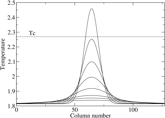
Figure 1: The time dependent Gaussian temperature profile used to simulate the decay of a laser heat pulse applied at the center line of the Ising lattice. The times plotted are $t=1$, 10, 25, 50, 100, 200, 300, and 500 MCSS. The tallest Gaussian corresponds to $t=1$ MCSS.

In the present paper we use a two-dimensional Ising ferromagnet to model the HAMR process by kinetic Monte Carlo (MC) simulation, demonstrating enhanced nucleation of the switched magnetization state in the heated area. For simplicity and computational economy, we envisage an experimental setup slightly different from others previously reported in the literature.Saga et al. (1999); Matsumoto et al. (2006); Waseda et al. (2008); Purnama et al. (2009) It most closely resembles the optical-dominant setup shown in Fig. 1(b) of Ref. Matsumoto et al., 2006. The recording medium is placed in a constant write field that is too weak to cause significant switching on an acceptable time scale, and it is heated at its center by a transient heat pulse. At a fixed superheating temperature we show that the relative speed-up of the magnetization switching, compared to the constant-temperature case, depends nonmonotonically on the magnitude of the applied field. This relative speed-up shows a pronounced maximum at an intermediate value of the applied field. We give a physical explanation for this effect, based on the nucleation theory of magnetization switching in finite-sized systems.Richards et al. (1995, 1996); Rikvold et al. (1994) As magnetization switching is a special case of the decay of a metastable phase (i.e., the medium in its state of magnetization opposite to the applied field),Rikvold et al. (1994); Rikvold and Gorman (1994) this analysis is of general physical interest beyond the specific technological application discussed here.

The rest of this paper is organized as follows. Our model and methods are described in Sec. II, the numerical results are described and explained in Sec. III, and our conclusions are stated in Sec. IV.

II Model and Methods

We use a square-lattice, nearest-neighbor Ising ferromagnet with energy given by the Hamiltonian,

$$\mathcal{H}=-J\sum_{\langle i,j\rangle}s_{i}s_{j}-H\sum_{i}s_{i}\;.$$ (1)

Here, $s_{i}=\pm 1$, $J>0$ is the strength of the spin interactions, and the first sum runs over all nearest-neighbor pairs. For convenience we hereafter set $J=1$. In the second term, which represents the Zeeman energy, $H$ is proportional to a uniform external magnetic field, and the sum runs over all lattice sites. We use a lattice of size $L^{2}=128\times 128$, with periodic boundary conditions. The length unit used in this study is the computational lattice constant, which should correspond to a few nanometers.

For simplicity, our model does not include any explicit randomness, such as impurities or random interaction strengths. As a result, pinning of interfaces for very weak applied field,Kirilyuk et al. (1997); Robb et al. (2008) as well as heterogeneous nucleation of spin reversalKirilyuk et al. (1997) are neglected. We further exclude demagnetizing effects, which are very weak for ultrathin filmsBander and Mills (1988); Back et al. (1995); Robb et al. (2008) and thus cause no qualitative changes in Monte Carlo simulations of the switching process.Richards et al. (1996)

The stochastic spin dynamic is given by the single-spin flip Metropolis algorithm with transition probabilityMetropolis et al. (1953)

$$P(s_{i}\rightarrow-s_{i})=\min[1,\exp(-\Delta E/T)]\;,$$ (2)

where $\Delta E$ is the energy change that would result from acceptance of the proposed spin flip. The temperature, $T$, is given in energy units (i.e., Boltzmann’s constant is taken as unity). Updates are attempted for randomly chosen spins, and $L^{2}$ attempts constitute one MC step per spin (MCSS), which is the time unit used in this work. (We note that the Metropolis algorithm is not the only Monte Carlo dynamics that could be used here. We have chosen it because of its simplicity and ubiquity in the literature since we do not expect that the inclusion of complications such intrinsic barriers to single-spin flips would have significant effects at this high temperature beyond a renormalization of the overall timescale.)

Following this algorithm and starting from $s_{i}=-1$ for all $i$, we equilibrate the system over $4\times 10^{4}$ MCSS at $H=0$ and temperature $T_{0}=0.8T_{c}\approx 1.82$, where $T_{c}=2/\ln(1+\sqrt{2})=2.269...$ is the exact critical temperature for the square-lattice Ising model.Onsager (1944) Having achieved equilibrium with negative magnetization at zero field, we then subject the system to a constant, uniform, positive magnetic field, along with a transient heat pulse. To simulate the heat pulse, we use a temperature profile given by a time-dependent, Gaussian solution of a one-dimensional diffusion equation. The profile is centered on the mid-line of the Ising lattice, $\bar{x}=63.5$, and each spin in the $x$th column of the lattice has the temperature

$$T(x,t)=T_{0}+0.3T_{c}\frac{t_{0}}{t+t_{0}}\exp\left(-\frac{(x-\bar{x})^{2}}{4k(t+t_{0})}\right),\;\;t\geq 0\;.$$ (3)

Here, $0.3T_{c}$ is the maximum of the temperature pulse, which is attained at $t=0$. Therefore, the peak temperature is $T_{0}+0.3T_{c}=1.1T_{c}$. The parameter $k$ is the thermal diffusivity, which is also set to unity for convenience. The time $t_{0}=\sigma^{2}/2k$ is related to the duration of the heat-input process, such that $\sigma$ is the standard deviation that governs the width of the temperature profile at $t=0$.Thompson (2009) Here we use $\sigma=6$ for all simulations. (Equation 3 most likely underestimates the speed of decay of the temperature pulse as it ignores heat conduction into the substrate.) Figure 1 displays the temperature of each column at eight times between $t=1$ and 500 MCSS. By first promoting the center-most lattice sites to temperatures above $T_{c}$ before relaxing them back to $T_{0}$ according to Eq. (3), we expect to initiate a magnetization-switching event that originates along the center line of the lattice and propagates outward. After the completion of this switching process, almost all spins will be oriented up, $s_{i}=+1$. We define the switching time $t_{\rm s}$ as the time until the system first reaches a magnetization per spin,

$$m=\frac{1}{L^{2}}\sum_{i}s_{i}\;,$$ (4)

of zero or greater.

III RESULTS

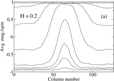
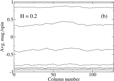
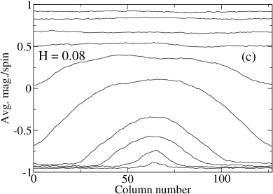
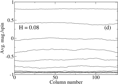
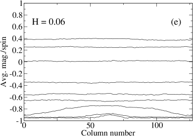
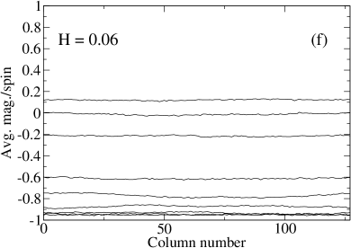
Figure 3: The magnetization per spin vs. the column number in the lattice, each part [(a)–(f)] averaged over 100 independent runs. The plots on the left [(a), (c), and (e)] result from the 100 runs with the relaxing temperature profile, and the ones on the right [(b), (d), and (f)] from the 100 runs at a constant, uniform temperature, $T_{0}=0.8T_{c}$. The plots at $H=0.2$ [(a) and (b)] show the average magnetization per spin at $t=1$, 10, 25, 50, 100, 150, 200, and 300 MCSS from bottom to top. The plots at $H=0.08$ [(c) and (d)] show the average magnetization per spin at $t=1$, 75, 400, 600, 1000, 1300, 1600, 2000, 3000, and 5500 MCSS from bottom to top. The plots at $H=0.06$ [(e) and (f)] show the average magnetization per spin at $t=1$, 500, 1500, 2500, 4000, 7500, 14000, 20000, and 25000 MCSS.

We first performed a preliminary study to confirm that magnetization switching can be induced by the temperature profile, given the parameters used in Eq. (3). For this purpose, we inspected snapshots of the system during a single run at $H=0.2$. In Fig. 2 we display the configuration of the system at six times between $t=1$ and 125 MCSS during this run. As expected, the switching begins near the center line of the system, where the temperature is above critical, and propagates outward. We note a strong similarity of the simulated magnetization configurations to experimental images of ultrathin, strongly anisotropic films undergoing magnetization reversal, such as Figs. 3, 4, and 8 of Ref. Kirilyuk et al., 1997 and Fig. 2 of Ref. Robb et al., 2008. This observation further confirms the ability of our simplified model to elucidate generic dynamical features of real ultrathin films.

Having confirmed a switching event at $H=0.2$, statistics were accumulated for 200 simulations at $H=0.2$ and also at fifteen weaker fields down to $H=0.06$, as detailed in Table 1. For each field, 100 simulations were performed at a constant, uniform temperature of $T_{0}=0.8T_{c}$, and 100 were performed using the time-dependent temperature profile given by Eq. (3). For each run, the average magnetization for each column at each time step was recorded along with the switching time, $t_{\rm s}$.

To investigate the effect that the relaxing temperature profile has on each column of the Ising lattice, we plotted the average magnetization per spin against the column number. In Fig. 3 we show this average magnetization for $H=$ 0.2, 0.08, and 0.06. The plots on the left [Fig. 3(a), (c), and (e)] result from the 100 runs with the relaxing temperature profile, and the ones on the right [Fig. 3(b), (d), and (f)] from the 100 runs at the constant, uniform temperature of $T_{0}$. The plots at $H=0.2$ [(a) and (b)] show the average magnetization per spin at eight different times between $t=1$ and 300 MCSS. The plots at $H=0.08$ [(c) and (d)] show the average magnetization per spin at ten different times between $t=1$ and 5500 MCSS. Finally, the plots at $H=0.06$ [(e) and (f)] show the average magnetization per spin at nine different times between $t=1$ and 25000 MCSS. (For a full listing of the times, see the figure caption.)

Again comparing the results with a relaxing temperature profile to those realized at constant, uniform temperature, in Fig. 4 we show cumulative probability distributions for the switching times for fields $H=0.2$, 0.15, 0.08, 0.0725, 0.065, and 0.06. The black “stairs” are the cumulative distributions for the switching times in the 100 runs with the relaxing temperature profile (hereafter referred to as $t_{\rm s}$). The gray (red online) stairs are the cumulative distributions for the switching times in the 100 runs at constant, uniform temperature (hereafter referred to as $t_{\rm c}$).

Table 1 lists the median switching times for both the 100 runs with the relaxing temperature profile ($t_{\rm s}$) and the 100 runs at constant, uniform temperature $T_{0}$ ($t_{\rm c}$) for each value of $H$. Also listed are the estimated errors $\Delta t_{\rm s}$ and $\Delta t_{\rm c}$. The last two columns give the ratio $t_{\rm s}/t_{\rm c}$ and the associated error $\Delta({t_{\rm s}}/{t_{\rm c}})$. The error $\Delta t_{\rm s}$ is defined as $(t_{{\rm s}2}-t_{{\rm s}1})/2$, where $t_{{\rm s}2}$ is the switching time with a cumulative probability of $0.55$ and $t_{{\rm s}1}$ is the switching time with a cumulative probability of $0.45$, and $\Delta t_{\rm c}$ is defined analogously. The error in the ratio $({t_{\rm s}}/{t_{\rm c}})$ is calculated in the standard way as

$$\Delta\left(\frac{t_{s}}{t_{c}}\right)=\sqrt{\left(\frac{\Delta t_{s}}{t_{c}}\right)^{2}+\left(\frac{t_{s}}{t_{c}^{2}}\Delta t_{c}\right)^{2}}\;.$$ (5)

The median switching time has the advantage over the mean that it can be estimated even when only half of the 100 simulations switch within the maximum number of time steps. This significantly reduces the computational requirements, especially for weak fields.

The ratio $({t_{\rm s}}/{t_{\rm c}})$ is plotted vs. $H$ in Fig. 5. The minimum value of this ratio signifies the maximum benefit from using the relaxing temperature profile of the HAMR method. The corresponding field value, $H=0.0725$, is the optimal field for this simulation.

To explain the nonmonotonic shape of the curve representing $({t_{\rm s}}/{t_{\rm c}})$ in Fig. 5, it is necessary to understand the two most important modes of nucleation-initiated magnetization switching in finite-sized systems: multidroplet (MD) and single-droplet (SD). (For more detailed discussions, see Refs. Rikvold et al., 1994; Rikvold and Gorman, 1994.) The average time between random nucleation events of a growing droplet of the equilibrium phase in a $d$-dimensional system of linear size $L$ has the strongly field-dependent form, $\tau_{\rm n}\propto L^{d}\exp[\Xi(T)/(T|H^{d-1}|)]$, where $\Xi(T)$ is a measure of the free energy associated with the droplet surface.Rikvold et al. (1994) Once a droplet has nucleated, for the weak fields and relatively high temperatures studied in this work it grows with a near-constant and isotropic radial velocity $v_{\rm g}\propto|H|/T$.Rikvold and Kolesik (2000) As a consequence, the time it would take a newly nucleated droplet to grow to fill half of a system of volume of $L^{d}$ is therefore $\tau_{\rm g}\propto L/v_{\rm g}$. If $\tau_{\rm g}\gg\tau_{\rm n}$, many droplets will nucleate before the first one grows to a size comparable to the system, and many droplets will contribute to the switching process. This is the MD regime, which corresponds to moderately strong fields and/or large systems.Rikvold et al. (1994) It is the switching mode shown in Fig. 2 for $H=0.2$. In the limit of infinitely large systems it is identical to the well-known Kolmogorov-Johnson-Mehl-Avrami (KJMA) theory of phase transformations.Kolmogorov (1937); Johnson and Mehl (1939); Avrami (1939); Ramos et al. (1999) If $\tau_{\rm g}\ll\tau_{\rm n}$, the first droplet to nucleate will switch the system magnetization on its own. This is the SD regime, which corresponds to weak fields and/or small systems.Rikvold et al. (1994) It is the switching mode shown in Fig. 6 for $H=0.06$. The crossover region between the SD and MD regimes is known as the Dynamic Spinodal (DSP).Rikvold et al. (1994)

One aspect of the MD/SD picture that is particularly relevant to the current problem, is the fact that any switching event that takes place at a time $t<\tau_{\rm g}$ cannot be accomplished by a single droplet, and thus it must be due to the MD mechanism.Brown et al. (2001) For a circular droplet in a square $L\times L$ system, $\tau_{\rm g}\approx L/(\sqrt{2\pi}v_{\rm g})$. Using results from Ref. Rikvold and Kolesik, 2000 (which, like the present model, neglects pinning effectsKirilyuk et al. (1997); Robb et al. (2008)), we find that in the range of moderately weak fields studied here, at $T=0.8T_{c}$ $v_{\rm g}$ can be well approximated as $v_{\rm g}\approx 0.75\tanh{(H/1.82)}$. The resulting estimates for $\tau_{\rm g}$ in the simulations (which contain no adjustable parameters) are shown as vertical lines in Fig. 4(c-f). A kink in the cumulative probability distribution for the heat-assisted runs is observed at $\tau_{\rm g}$, with significantly higher slopes in the MD regime on the short-time side of $\tau_{\rm g}$, than in the SD regime on the long-time side. From these figures we see that the optimal field value for $L=128$, $H=0.0725$, corresponds to the situation where just above 50% of the heat-assisted switching events are caused by the MD mechanism, while essentially all the constant-temperature switching events are SD. This situation is illustrated by the series of snapshots in Fig. 7. For significantly larger fields, both protocols lead to all MD switching events [Fig. 4(a,b)], while for weaker fields, the great majority of the switching events are SD for both protocols [Fig. 4(e,f)]. In both cases, the ratio $t_{\rm s}/t_{\rm c}$ is larger than it is for fields near the optimal value [Fig. 4(c,d)]. We have confirmed these conclusions by additional simulations for $L=64$ and 96 (not shown).

IV Conclusions

In this paper we have studied a kinetic Ising model of magnetization reversal under the influence of a momentary, spatially localized input of energy in the form of heat (heat-assisted magnetization reversal, or HAMR). Our numerical results indicate that the HAMR technique can significantly speed up the magnetization reversal in a uniform, applied magnetic field, and we find that this speed-up has its optimal value at intermediate values of the field. This effect is explained in terms of the MD and SD mechanisms of nucleation-initiated magnetization switching in finite systems.Rikvold et al. (1994) The two-dimensional geometry chosen for this study is particularly appropriate for thin films. We therefore expect that our predictions should be experimentally observable for ultrathin ferromagnetic films with strong perpendicular anisotropy, such as Co/PdCarcia et al. (1985); Purnama et al. (2009) or Co/PtRobb et al. (2008); Ferré (2002) multilayers.

Table 1: Median switching times $t_{\rm s}$ (relaxing temperature profile) and $t_{\rm c}$ (constant, uniform temperature) and their ratio for the sixteen field values included in Fig. 5. Also given are the estimated errors, $\Delta t_{\rm s}$, $\Delta t_{\rm c}$, and $\Delta(t_{\rm s}/t_{\rm c})$.

$H$	Median $t_{\rm s}$	$\Delta t_{\rm s}$	Median $t_{\rm c}$	$\Delta t_{\rm c}$	$(t_{\rm s}/t_{\rm c})$	$\Delta(t_{\rm s}/t_{\rm c})$
0.2000	98.0	1.0	126.0	1.5	0.778	0.012
0.1800	126.0	1.5	166.5	2.0	0.757	0.013
0.1600	165.0	0.5	225.5	4.0	0.732	0.013
0.1500	189.5	2.5	263.0	4.5	0.721	0.016
0.1200	323.0	6.0	482.5	6.5	0.669	0.015
0.1000	504.0	16.0	881.5	25.0	0.572	0.024
0.0900	670.5	14.5	1253.0	92.0	0.535	0.041
0.0800	1077.0	43.0	2015.0	113.0	0.534	0.037
0.0775	1148.0	72.0	2676.0	344.5	0.429	0.061
0.0725	1374.0	63.5	4413.0	354.5	0.311	0.029
0.0700	2443.0	274.5	5470.0	938.0	0.447	0.092
0.0670	3232.0	629.5	6621.5	838.5	0.488	0.113
0.0660	4035.5	580.5	7562.5	733.0	0.534	0.093
0.0650	6426.5	1453.0	9030.0	1035.5	0.712	0.180
0.0620	11569.5	1927.0	14788.0	3607.0	0.782	0.231
0.0600	13808.0	2479.0	20851.0	3435.5	0.662	0.161

Figure 2: Parts (a)-(f) are snapshots of the $128\times 128$ Ising system at $t=1$, 10, 25, 50, 100, and 125 MCSS under influence of the time-dependent temperature profile, Eq. (3), and a constant, uniform applied field of $H=0.2$. Growing clusters of the switched phase are first seen to nucleate near the center line, where the temperature is highest. However, active nucleation is also seen elsewhere in the system.

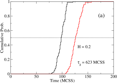
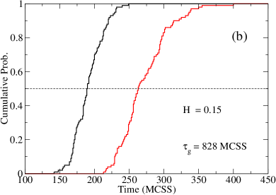
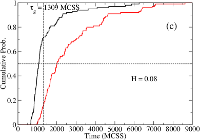
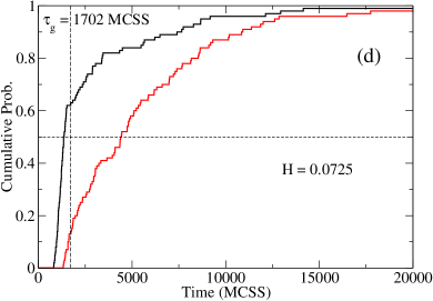
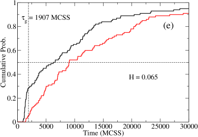
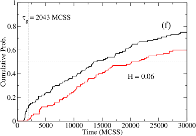
Figure 4: Parts (a) – (f) are cumulative probability distributions for the switching times with fields $H=0.2$, 0.15, 0.08, 0.0725, 0.065, and 0.06, respectively. The black “stairs” correspond to the 100 simulations with the relaxing temperature profile (switching times, $t_{\rm s}$). The gray (red online) stairs correspond to the 100 simulations at uniform temperature (switching times, $t_{\rm c}$). The vertical lines in parts (c) – (f) mark the single-droplet growth time $\tau_{\rm g}$. Note that the time scale increases by more than a factor 100 from (a) to (f). See discussion in the text.

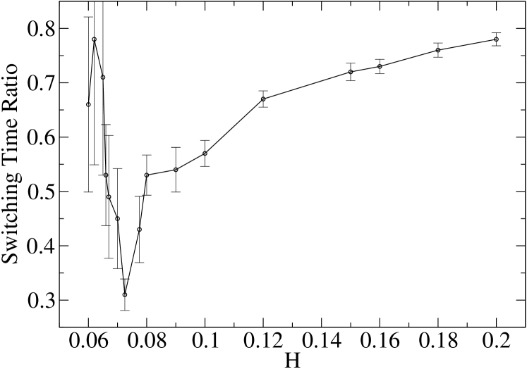
Figure 5: The switching-time ratio $t_{\rm s}/t_{\rm c}$, shown vs. $H$. The minimum value of this ratio signifies the maximum benefit from applying the relaxing temperature profile of the HAMR method.

Figure 6: Parts (a)-(d) are snapshots of the $128\times 128$ Ising system at $t=1$, 500, 1500, and 2500 MCSS under influence of the time-dependent temperature profile, Eq. (3), and a constant, uniform applied field of $H=0.06$. In this weak field the switching follows the SD mechanism, even in the heated region.

Figure 7: Parts (a)-(f) are snapshots of the $128\times 128$ Ising system at $t=1$, 200, 400, 600, 800, and 1000 MCSS under influence of the time-dependent temperature profile, Eq. (3), and a constant, uniform applied field of $H=0.075$. At this intermediate field, multiple growing clusters of the switched phase are first seen to nucleate near the center line, where the temperature is highest. Without the heat pulse, the switching would proceed via the SD mechanism.

References

- McDaniel (2005) T. W. McDaniel, J. Phys.: Condens. Matter 17, R315 (2005).
- Bean and Livingston (1959) C. P. Bean and J. D. Livingston, J. Appl. Phys. 30, 120S (1959).
- Richards et al. (1995) H. L. Richards, S. W. Sides, M. A. Novotny, and P. A. Rikvold, J. Magn. Magn. Mater. 150, 37 (1995).
- Matsumoto et al. (2006) K. Matsumoto, A. Inomata, and S. Hasegawa, FUJITSU Sci. Tech. J. 42, 158 (2006).
- Saga et al. (1999) H. Saga, H. Nemoto, H. Sukeda, and M. Takahashi, Jpn. J. Appl. Phys. 38, 1839 (1999).
- Katayama et al. (2000) H. Katayama, M. Hamamoto, J. Sato, Y. Murakami, and K. Kojima, IEEE Trans. Magn. 36, 195 (2000).
- Purnama et al. (2007) B. Purnama, Y. Nozaki, and K. Matsuyama, J. Magn. Magn. Mater. 310, 2683 (2007).
- Waseda et al. (2008) K. Waseda, R. Doi, B. Purnama, S. Yoshimura, Y. Nozaki, and K. Matsuyama, IEEE Trans. Magn. 44, 2483 (2008).
- Purnama et al. (2009) B. Purnama, T. Tanaka, Y. Nozaki, and K. Matsuyama, Appl. Phys. Express 2, 033001 (2009).
- Challener et al. (2009) W. A. Challener, C. Peng, A. V. Vitagi, D. Karns, W. Peng, Y. Peng, X. M. Yang, X. Zhu, N. J. Gokemeijer, Y.-T. Hsia, G. Ju, R. E. Rottmayer, M. A. Seigler, and E. C. Gage, Nature Photonics 3, 220 (2009).
- Stipe et al. (2010) B. C. Stipe, T. C. Strand, C. C. Poon, H. Balamane, T. D. Boone, J. A. Katine, J.-L. Li, V. Rawat, H. Nemoto, A. Hirotsune, O. Hellwig, R. Ruiz, E. Dobisz, D. S. Kercher, N. Robertson, T. R. Albrecht, and B. D. Terris, Nature Photonics 4, 484 (2010).
- O’Connor and Zayats (2010) D. O’Connor and A. V. Zayats, Nature Nanotechnology 5, 482 (2010).
- Bander and Mills (1988) M. Bander and D. L. Mills, Phys. Rev. B 38, 12015 (1988).
- Back et al. (1995) C. Back, C. Würsch, A. Vaterlaus, U. Ramsperger, U. Maier, and D. Pescia, Nature (London) 378, 597 (1995).
- Kirilyuk et al. (1997) A. Kirilyuk, F. Ferré, V. Grolier, J. P. Jamet, and D. Renard, J. Magn. Magn. Mater. 171, 45 (1997).
- Robb et al. (2008) D. T. Robb, Y. H. Xu, O. Hellwig, J. McCord, A. Berger, M. A. Novotny, and P. A. Rikvold, Phys. Rev. B 78, 134422 (2008).
- Carcia et al. (1985) P. F. Carcia, A. D. Meinhaldt, and A. Suna, Appl. Phys. Lett. 47, 178 (1985).
- Ferré (2002) F. Ferré, in Spin Dynamics in Confined Magnetic Structures I, edited by B. Hillebrands and K. Ounadjela (Springer-Verlag, Berlin Heidelberg, 2002), pp. 127–168, Topics in Applied Physics, Vol. 83.
- Lyberatos (2000) A. Lyberatos, J. Phys. D: Appl. Phys. 33, R117 (2000).
- Richards et al. (1996) H. L. Richards, M. A. Novotny, and P. A. Rikvold, Phys. Rev. B 54, 4113 (1996).
- Rikvold et al. (1994) P. A. Rikvold, H. Tomita, S. Miyashita, and S. W. Sides, Phys. Rev. E 49, 5080 (1994).
- Rikvold and Gorman (1994) P. A. Rikvold and B. M. Gorman, in Annual Reviews of Computational Physics I, edited by D. Stauffer (World Scientific, Singapore, 1994), pp. 149–191.
- Metropolis et al. (1953) N. Metropolis, A. W. Rosenbluth, M. N. Rosenbluth, A. H. Teller, and E. Teller, J. Chem. Phys. 21, 1087 (1953).
- Onsager (1944) L. Onsager, Phys. Rev. 65, 117 (1944).
- Thompson (2009) S. H. Thompson, Computational and Analytical Studies of Magnetization Switching in Iron Nanopillars (Ph. D. Dissertation. Florida State University, Tallahassee, FL, 2009), Ch. 5. http://etd.lib.fsu.edu.proxy.lib.fsu.edu/theses/available/etd-03272009-144735/.
- Rikvold and Kolesik (2000) P. A. Rikvold and M. Kolesik, J. Stat. Phys. 100, 377 (2000).
- Kolmogorov (1937) A. N. Kolmogorov, Bull. Acad. Sci. USSR, Phys. Ser. 1, 355 (1937).
- Johnson and Mehl (1939) W. A. Johnson and R. F. Mehl, Trans. Am. Inst. Mining and Metallurgical Engineers 135, 416 (1939).
- Avrami (1939) M. Avrami, J. Chem. Phys. 7, 1103 (1939); 8, 212 (1940); 9, 177 (1941).
- Ramos et al. (1999) R. A. Ramos, P. A. Rikvold, and M. A. Novotny, Phys. Rev. B 59, 9053 (1999).
- Brown et al. (2001) G. Brown, M. A. Novotny, and P. A. Rikvold, Phys. Rev. B 64, 134422 (2001).