Imperial-TP-2011-ND-02
NSF-KITP-11-073
AEI-2011-027

$\to$      $\to$   

Nadav Drukker and Valentina Forini
^aThe Blackett Laboratory, Imperial College London,
Prince Consort Road, London SW7 2AZ, U.K.
^bMax-Planck-Institut für Gravitationsphysik, Albert-Einstein-Institut,
Am Mühlenberg 1, D-14476 Potsdam, Germany

Generalized quark-antiquark potential
at weak and strong coupling

1 Introduction

The duality between ${\mathcal{N}}=4$ SYM in four dimensions and type IIB string theory on $AdS_{5}\times\mathbb{S}^{5}$ has gone through a revolution in the past few years. From the early study of general features, protected quantities and BPS observables, it evolved into the precision study of the spectrum of local operators and of scattering amplitudes. In both these examples the (conjectured) integrability of the planar theory enabled great calculational leaps allowing in certain cases to find non-trivial interpolating functions matching all known explicit weak and strong coupling tests as well as satisfying very restrictive consistency conditions.

A natural family of observables in the gauge theory are Wilson loops, realized in the dual theory as infinite open strings. When the asymptotic boundary is along light–like segments, they are related by T-duality to scattering amplitudes [1]. The most natural Wilson loop, though, is a pair of antiparallel lines in flat space, which calculates the effective potential between a pair of infinitely heavy W-boson probes.

The expectation value of this observable was calculated very early after the introduction of the $AdS$/CFT duality by a classical string configuration [2, 3]. Since then very little progress has been made in understanding this quantity. It has been calculated at weak coupling to second order in perturbation theory [4, 5, 6] and on the string theory side the problem of calculating the first correction (of relative order $\lambda^{-1/2}$) was formulated in [7, 8], evaluated numerically in [9] and simplified further in [10] to an analytic one–dimensional integral.

As it turned out, the circular Wilson loop is a much simpler observable, which in the Feynman gauge receives contributions only from ladder graphs [5, 11, 12]. For the antiparallel lines the ladder graphs give an answer of the same order as that calculated by string theory, but not identical [4, 5].

We examine here this problem again and propose a program which may allow for an exact calculation of the expectation value of such unprotected Wilson loops at all values of the coupling.

Since ${\mathcal{N}}=4$ SYM is conformal, the potential calculated by the Wilson loop has the Coulomb form with a coefficient which is coupling dependent. It would be very useful to introduce extra parameters to the problem which one could vary to get a handle on the calculation. In fact there are two simple deformations of the problem which do not make the perturbative or supergravity calculation any harder and allow to interpolate between protected operators and the desired observable.

The first deformation parameter was introduced already in [2], and allows for the two lines to couple to two different scalar fields. We label this parameter $\theta$. For $\theta=0$ the two lines couple to the same scalar field, say $\Phi_{1}$. When $\theta=\pi/2$ the two lines couple to $\Phi_{1}\pm\Phi_{2}$, which are orthogonal to each-other. Then for $\theta=\pi$ they couple to the field $\Phi_{2}$, but with opposite signs, which means that the lines are effectively parallel, rather than antiparallel. In that case the two lines share eight supercharges and the correlator is trivial.

The other deformation parameter is geometric. One way to illustrate it is to replace the theory on $\mathbb{R}^{4}$ with the theory on $\mathbb{S}^{3}\times\mathbb{R}$ (related by the exponential map). Now we consider a pair of antiparallel lines separated by an angle $\pi-\phi$ on $\mathbb{S}^{3}$. For $\phi=0$ the two lines are antipodal and mutually BPS, while for $\phi\to\pi$ the lines get very close together. If we “zoom in” to the vicinity of the lines by a conformal transformation we get a situation very similar to the original antiparallel lines in flat space.

Different points of view on this deformation are presented in the following section, and the $\phi\to\pi$ limit is explored in more detail in Section 5. Let us note here only that an equivalent picture is that of a cusp in the plane in $\mathbb{R}^{4}$. For $\phi=0$ the cusp disappears and the system is that of a single infinite straight line.

Going back to the $\mathbb{S}^{3}\times\mathbb{R}$ picture, the expectation value of the Wilson loop calculates the effective potential $V(\phi,\theta,\lambda)$ between a generalized quark antiquark pair, in exactly the same way as originally proposed by Wilson [13]. The operator is made of a pair of lines extending over a large time $T$ and can be written as

$$W=\frac{1}{N}\operatorname{Tr}{\mathcal{P}}\exp\left[\oint(iA_{\mu}\dot{x}^{\mu}+\Phi_{I}\Theta^{I}|\dot{x}|)ds\right].$$ (1.1)

The expectation value of the loop operator has the behavior

$${\left<{W}\right>}\approx\exp\Big{[}{-}T\,V(\phi,\theta,\lambda)\Big{]}\,.$$ (1.2)

The effective potential $V(\phi,\theta,\lambda)$ depends on the ’t Hooft coupling $\lambda=g^{2}N$ (we do not consider non-planar corrections) and it can be expanded at weak coupling in a perturbative series

$$V(\phi,\theta,\lambda)=\sum_{n=1}^{\infty}\left(\frac{\lambda}{16\pi^{2}}\right)^{n}V^{(n)}(\phi,\theta)\,.$$ (1.3)

In section 3 we present the exact form of the first two terms in this expansion, based on [14].

The strong coupling behavior of $V(\phi,\theta,\lambda)$ can be calculated in a systematic expansion around a classical string solution. The function is expected to have an asymptotic expansion of the form

$$V(\phi,\theta,\lambda)=\frac{\sqrt{\lambda}}{4\pi}\sum_{l=0}^{\infty}\left(\frac{4\pi}{\sqrt{\lambda}}\right)^{l}V_{AdS}^{(l)}(\phi,\theta)\,.$$ (1.4)

In Section 4 we study this expansion. $V_{AdS}^{(0)}$ is proportional to the classical action of the string solution, calculated originally in [15, 16]. The next term, $V_{AdS}^{(1)}$, requires tracing over all fluctuation modes and we derive an integral expression which can be evaluated numerically to high precision for fixed $\phi$ and $\theta$.

The coefficients in the perturbative expansions are complicated functions of the angles $\phi$ and $\theta$ and at strong coupling they are given only implicitly (at the classical level) or in integral form (one–loop). We consider therefore the expansion of these functions around $\phi=\theta=0$. This is an expansion around the $1/2$ BPS line (or circle), one of the most simple observables in the theory. We view the general problem as a deformation of this $1/2$ BPS configuration and use the fact that a deformation of a Wilson loop can be written in terms of insertions of local operators into the loop.

Changing $\phi$, which modifies the path of the loop is captured by insertions of the field strength $F_{\mu\nu}$, as well as its derivatives, into the Wilson loop. Somewhat simpler is to change $\theta$ which introduces local scalar field insertions into the loop. Both these quantities can be calculated perturbatively, the relevant graphs come from limits of the graphs calculating the effective potential at finite values of $\phi$ and $\theta$. On the string side we are also able to get exact analytical results for the expansion coefficients, by inverting certain transcendental functions perturbatively and from the expansion of elliptic functions at small modulus in terms of trigonometric functions, which simplifies the integrals arising at one–loop.

In Section 6 we present these expansions and explore some of their properties. In particular, we can identify specific diagrams in perturbation theory contributing to the different terms in the expansion.

We end with a discussion of our results.

For the benefit of the casual reader, we have tried to keep the body of the paper focused on presenting and analyzing our results. The derivation of these results is presented in many appendices, dedicated to perturbation theory, classical string calculations, the one–loop determinants and their various limits.

2 Setup

We would like to present more details about the different ways we can view the Wilson loop observables we will study in the rest of the paper.

Figure 1: Antiparallel lines on $\mathbb{S}^{3}\times\mathbb{R}$ with Lorentzian signature can be mapped by different conformal transformations to hyperbolas in Minkowski space, arranged so that they all pass through the points $\pm 1$ on the horisontal axis. The thin lines on the cylinder map to the boundary of Minkowski space.

We start by considering the gauge theory on $\mathbb{S}^{3}\times\mathbb{R}$. The loop is made of two lines separated by an angle $\pi-\phi$ along a big circle on $\mathbb{S}^{3}$. Parameterizing the angle along this circle by $\varphi$ and the time direction by $t$ we have a pairs of lines, one going in the future direction and one to the past. The parameters appearing in the Wilson loop (1.1) are therefore

$$t =s\,, \qquad\varphi =\frac{\phi}{2}\,, \qquad\Theta^{1} =\cos\frac{\theta}{2}\,, \qquad\Theta^{2} =\sin\frac{\theta}{2}\,,$$ (2.1)

$$t =-s^{\prime}\,, \qquad\varphi =\pi-\frac{\phi}{2}\,, \qquad\Theta^{1} =\cos\frac{\theta}{2}\,, \qquad\Theta^{2} =-\sin\frac{\theta}{2}\,.$$

It is natural (in particular in the context of $AdS$) to use Lorentzian signature on this space. A conformal transformation maps a region of $\mathbb{S}^{3}\times\mathbb{R}$ to the entire 4d Minkowski space. A straight time–like line gets mapped under this transformation to a hyperbola, in the same way that in Euclidean space lines get mapped to circles. A Wilson line along such a curve is $1/2$ BPS [17]. The same is true for a pair of hyperbolas sharing the same focal point, as they are the image of two antipodal lines on the $\mathbb{S}^{3}\times\mathbb{R}$. In all other cases the conformal transformation to Minkowski space will give a pair of hyperbola which do not satisfy this property and are not mutually BPS. In the limit of $\phi\to\pi$, where the separation of the two lines on the cylinder is $\pi-\phi$, the two hyperbola look at the vicinity of the origin like two antiparallel lines. See Figure 1.

If we Wick-rotate $\mathbb{S}^{3}\times\mathbb{R}$ to Euclidean signature, then we can use the exponential map to get flat Euclidean space. The pairs of lines running along the time direction get mapped to rays intersecting at the origin. The angle between the rays is $\pi-\phi$, such that for $\phi=0$ they form a continuous straight line. Otherwise there is a singular point.

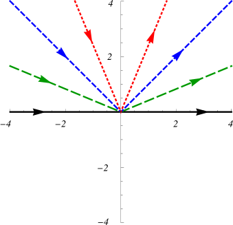
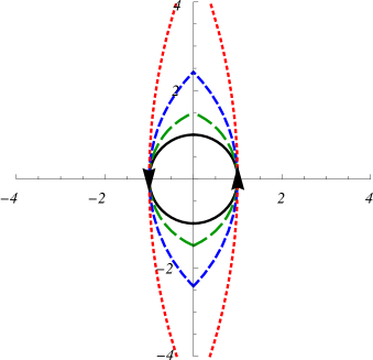
Figure 2: Pairs of rays intersecting at angles $\phi=0,\pi/4,\pi/2,3\pi/4$ get mapped by different conformal transformations to pairs of intersecting arcs, interpolating between the circle and a pair of antiparallel lines.

In this picture the path is given by

$$x^{1}=s\cos\frac{\phi}{2}\,,\qquad x^{2}=|s|\sin\frac{\phi}{2}\,,\qquad\Theta^{1}=\cos\frac{\theta}{2}\,,\qquad\Theta^{2}=\operatorname{sign}(s)\sin\frac{\theta}{2}\,.$$ (2.2)

We can perform a conformal transformation which maps the point at infinity to finite distance, so the pair of rays get replaced by two arcs, intersecting at angle $\pi-\phi$, as in Figure 2. We can take them to be arcs of circles of radius $r=1/(1-\sin(\phi/2))$ centered at $\pm(r-1)$. These arcs pass through the points $\pm 1$. The distance between the two intersection points is $2r\cos(\phi/2)$ and diverges for $\phi\to\pi$ like $8/(\pi-\phi)$. In this limit the conformal transformation of the cusp approximates a pair of antiparallel lines.

Cusped Wilson loops suffer from logarithmic divergences [18, 19]. This is exactly the same as the linear time divergence of (1.2). The expectation value of the cusped loop is therefore

$${\left<{W_{\text{cusp}}}\right>}\approx\exp\Big{[}{-}\log(R/\epsilon)\,V(\phi,\theta,\lambda)\Big{]}\,.$$ (2.3)

The cutoffs of the two calculations are related by $\log(R/\epsilon)\sim T$.

In the case of the straight line, the conformal transformation gives the circle. Their expectation value is not the same, and this can be attributed to the large conformal transformation relating them [11]. The same is true for cusped loops, in the special cases when $\phi=\pm\theta$ [16] (see also [20, 21]). In these cases, the loop preserves some supercharges and is finite. Then this finite quantity is tractable, and indeed the only interesting quantity to calculate. For generic angles a divergence arises which completely masks this finite term. Still, one has to make sure that the same prescription and regularization is used for both calculations. This is particularly true in the Lorentzian case, where the conformal map eliminates more than one point from space.

In the limit that $\phi\to\pi$ there will be an extra pole in $V$, as the lines become coincident. The residue at this pole is the potential between a pair of antiparallel lines in flat space, as we discuss in Section 5.

3 Weak coupling

Instead of calculating the correlator of two lines on $\mathbb{S}^{3}\times\mathbb{R}$ we work with the cusp in $\mathbb{R}^{4}$. The logarithmic divergence arising from such singular points in the loop were discussed extensively (see e.g., [22, 18, 19, 23, 24, 25]).

Allowing for the extra angle $\theta$ in ${\mathcal{N}}=4$ SYM, the calculation of the potential $V^{(1)}$ at one–loop order was done in [15]. The result is

$$V^{(1)}(\phi,\theta)=-2\,\frac{\cos\theta-\cos\phi}{\sin\phi}\,\phi\,.$$ (3.1)

The extension to 2–loops in the case when $\theta=0$ was done in [14] (see also [23]). The resulting expressions were written in [14] in integral form, and in Appendix A we extend the expressions to $\theta\neq 0$ and compute the integrals in closed form. The result can be written as a sum of the contribution of ladder graphs (after subtracting the exponentiation of the $O(\lambda)$ term), and the interacting graphs

$$V^{(2)}(\phi,\theta) =V^{(2)}_{\text{lad}}(\phi,\theta)+V^{(2)}_{\text{int}}(\phi,\theta)$$ (3.2)

$$V^{(2)}_{\text{lad}}(\phi,\theta) =-4\,\frac{(\cos\theta-\cos\phi)^{2}}{\sin^{2}\phi}\left[\operatorname{Li}_{3}\left(e^{2i\phi}\right)-\zeta(3)-i\phi\left(\operatorname{Li}_{2}\left(e^{2i\phi}\right)+\frac{\pi^{2}}{6}\right)+\frac{i}{3}\phi^{3}\right],$$

$$V^{(2)}_{\text{int}}(\phi,\theta) =\frac{4}{3}\,\frac{\cos\theta-\cos\phi}{\sin\phi}\,(\pi-\phi)(\pi+\phi)\phi\,.$$

To check these analytic expressions, one can focus on the BPS case [26], when $\phi=\pm\theta$ and indeed $V^{(1)}=V^{(2)}=0$ as expected. As another test, for large imaginary angle the leading behavior is

$$V^{(1)}(iu,\theta) =2u+O(e^{-u})\,,$$ (3.3)

$$V^{(2)}(iu,\theta) =-\frac{2\pi^{2}}{3}u-4\,\zeta(3)+O(u^{-1})\,.$$

together we find

$$V(iu,\theta)=\left(\frac{\lambda}{8\pi^{2}}-\frac{\lambda^{2}}{384\pi^{2}}+O(\lambda^{3})\right)u+O(u^{0})\,,$$ (3.4)

and the prefactor of the linear term indeed matches a quarter of the perturbative expansion of the cusp anomalous dimension, $\gamma_{\text{cusp}}$ [27].

Note that both interacting and ladder graphs at this order have uniform transcendentality three (when $e^{2i\phi}$ is considered rational). It is rather interesting that the complicated interacting graphs give a result which is much simpler than the 2–loop ladder graph and does not involve polylogarithmic functions. Indeed it is proportional to the 1–loop result

$$V^{(2)}_{\text{int}}(\phi,\theta)=-\frac{2}{3}(\pi^{2}-\phi^{2})V^{(1)}(\phi,\theta)\,.$$ (3.5)

The fact that the prefactor $\cos\theta-\cos\phi$ (where all the $\theta$ dependence lies) is the same is obvious and can be seen also before integration. It is much more intriguing that the ratio of the final result of integration and $V^{(1)}$ is a polynomial in $\phi$.

In particular, in [14] an integral equation was written whose solution gives the contribution of ladder graphs to all orders in perturbation theory. If the interacting graphs are all related to lower order ladder graphs by some simple relations, it may be possible to find a full expression for $V(\phi,\theta,\lambda)$ for all values of the coupling.

Figure 3: Curves showing $V^{(1)}(\phi,0)$ (blue, wide dashes), $V^{(2)}(\phi,0)$ (green, dash-dot), $V^{(0)}_{AdS}(\phi,0)$ (red, short dashes) And $V^{(1)}_{AdS}(\phi,0)$ (purple, short dash-dot). Note that all have a simple pole at $\phi=\pi$, with different residues. The dotted lines show the perturbative expansions of $V^{(0)}_{AdS}$ and $V^{(1)}_{AdS}$ around $\phi=0$ to order $\phi^{8}$, (6.5), (6.6), which furnish a good approximation up to $\phi\sim 2$.

4 Strong coupling

In the strong coupling $AdS$ dual, Wilson loops are described by macroscopic strings [2, 3]. It is easy to write down the classical string solutions in $AdS_{5}\times\mathbb{S}^{5}$ describing these Wilson loops. For the gauge theory on $\mathbb{S}^{3}\times\mathbb{R}$ it is appropriate to use global Lorentzian $AdS_{5}$ and take an ansatz which is time independent. For the cusp in $\mathbb{R}^{4}$ it is more appropriate to consider the Euclidean Poincaré patch, in which case the ansatz posses a conformal symmetry. The solutions are clearly related by an isometry which is the bulk extension of the conformal transformation discussed in Section 2.

These classical solutions were written down in the case of $\theta=0$ in [15] and for $\theta\neq 0$ in Appendix C.2 of [16]. As we review in Appendix B, the classical solutions are expressed as functions of two parameters $q$ and $p$ (B.5) (or in terms of $b$ and $k$ (B.7), (B.8)) and can be found for arbitrary values of $\phi$ and $\theta$, as the solutions of transcendental equations.

The quadratic fluctuation Lagrangian can be written for all values of the parameters, see Appendix C. In two limits the mass matrix diagonalizes, which are for $\theta=0$ (equivalently $q=0$), and for $\phi=0$ (the limit $p\propto q\to\infty$). In both these cases (studied in Appendices D and E respectively) all the quadratic fluctuation operators can be written in the form of single gap Lamé differential operators. The determinants for each of these operators can be calculated analytically, using the Gelfand-Yaglom method. The full determinant which includes the contribution of the trivial time direction is then expressed as a single integral, see equations (D.41) and (E.20).

This is exactly the same form as was found for the case of the antiparallel lines in flat space in [10] and it can be readily evaluated numerically for arbitrary values of $\phi$ and $\theta$, see the short daash-dot (purple) line in Figure 3. In general we do not know how to calculate these integrals analytically, but we can evaluate them in a systematic expansion around $\theta=0$ and $\phi=0$.

Indeed, one motivation for studying this generalization of the antiparallel lines is that it would be easier to calculate it for $\theta\sim\phi\sim 0$ than for $\phi=\pi$. We present the results of these expansions in Section 6 below.

5 Antiparallel lines limit

As mentioned in the introduction, part of the motivation for this project is as a stepping stone to understanding the potential between two antiparallel lines in ${\mathcal{N}}=4$ SYM at all couplings. We introduced two deformation parameters, $\phi$ and $\theta$, and claimed that the original problem is recovered for $\phi\to\pi$ (and $\theta=0$).

To some degree this claim is obvious, one can look at figures 1 and 2, and see that for $\phi\to\pi$ the curves approach antiparallel lines. Yet, this approach to the problem introduces a specific regularization prescription. We therefore examine here the $\phi\to\pi$ limit in detail and see how to recover the usual result for antiparallel lines from it.

5.1 Weak coupling

Taking the $\phi\to\pi$ limit on the perturbative expressions (3.1) and (3.2) leads to a pole

$$V_{||}(\phi,\theta)\to-\frac{\lambda}{8\pi}\frac{1+\cos\theta}{\pi-\phi}+\frac{\lambda^{2}}{32\pi^{3}}\frac{(1+\cos\theta)^{2}}{\pi-\phi}\log\frac{e}{2(\pi-\phi)}+O(\lambda^{3})\,.$$ (5.1)

The potential between antiparallel lines was calculated for $\theta=0$ to two–loop order in [4]. The result found there is

$$V_{||}(0)=-\frac{\lambda}{4\pi L}+\frac{\lambda^{2}}{8\pi^{3}L}\log\frac{T}{L}+O(\lambda^{3})\,.$$ (5.2)

This behavior indeed matches the leading pole we find in (5.1), with the replacement $L\to\pi-\phi$. The extra logarithmic divergence at two–loop order breaks the scaling behavior expected for the Wilson loop. Such divergences were explained in [28] as arising from infrared effects, and get replaced by a logarithm of the coupling when including higher order soft–gluon graphs, see the more careful treatment in [6].

5.2 Strong coupling

We can look at the same limit at strong coupling. The classical solution is written down in Appendix B and one can see that the relevant limit is (B.5), (B.8)

$$p\to 0\,,\qquad\frac{q^{2}}{p}=\frac{1-2k^{2}}{k\sqrt{1-k^{2}}}\ \ \text{fixed.}\qquad 0<k<1.$$ (5.3)

$\phi$ (B.10) indeed approaches $\pi$

$$\pi-\phi=2\sqrt{p}\,\frac{{\mathbb{E}}-(1-k^{2}){\mathbb{K}}}{\sqrt{k}(1-k^{2})^{1/4}}\,,$$ (5.4)

where ${\mathbb{K}}={\mathbb{K}}(k^{2})$ and ${\mathbb{E}}={\mathbb{E}}(k^{2})$ are complete elliptic integrals of the first and second kind, see Appendix F for their definitions and some of their properties.

The expression for $\theta$ (B.14) is

$$\theta=2\sqrt{1-2k^{2}}\,{\mathbb{K}}$$ (5.5)

and the action (B.16) is

$$\lim_{\phi\to\pi}V_{AdS}^{(0)}(\phi,\theta) =-\frac{4}{\sqrt{p}}\frac{{\mathbb{E}}-(1-k^{2}){\mathbb{K}}}{\sqrt{k}(1-k^{2})^{1/4}}=-\frac{8}{\pi-\phi}\frac{\big{(}{\mathbb{E}}-(1-k^{2}){\mathbb{K}}\big{)}^{2}}{k\sqrt{1-k^{2}}}$$ (5.6)

This is exactly the result found in [2] (with $k^{2}\to(1-l^{2})/(2-l^{2})$ and $\pi-\phi\to L$ and a factor of 2 in the definition of $g_{YM}^{2}$).

Specializing to the case of $\theta=0$ we need to set $k^{2}=1/2$ and the elliptic integrals can be expressed in terms of $\Gamma\left(\frac{1}{4}\right)^{2}$. We then find

$$V_{AdS}^{(0)}(\phi,0)=-\frac{16\pi^{3}}{(\pi-\phi)\Gamma\left(\frac{1}{4}\right)^{4}}\,,$$ (5.7)

agreeing with the result of [2, 3] for the antiparallel lines in flat space with the replacement $\pi-\phi\to L$.

We can compare our calculation of the one–loop determinant in Appendix D with that performed for the parallel lines in [9, 10]. These papers studied the $\theta=0$ case, and the fluctuation operators there are the same as those in (D.5) for the case $k^{2}=1/2$. The two calculations do differ in the dependence on the time direction. After integrating over the world–sheet time direction we need to replace the cutoff on the world–sheet time $\cal T$ with the target space time $T$, which for $p\to 0$ is (B.23)

$$\frac{{\cal T}}{T}=\frac{1}{\sqrt{k}(1-k^{2})^{1/4}\sqrt{p}}=\frac{2}{\pi-\phi}\frac{{\mathbb{E}}-(1-k^{2}){\mathbb{K}}}{k\sqrt{1-k^{2}}}\,.$$ (5.8)

This factor gives the expected $1/(\pi-\phi)$ pole for generic $k$. In the case of $k^{2}=1/2$ the ratio is $\pi/(\pi-\phi){\mathbb{K}}(1/2)$, which upon the replacement $\pi-\phi\to L$, is indeed the rescaling done in [9, 10].

Thus, we see that the $\phi\to\pi$ limit does indeed reproduce the result for the antiparallel lines both at weak and strong coupling with the replacement of the pole $\pi-\phi\to L$.

6 Near straight–line expansion

The limit of $\phi\to\pi$ is interesting physically, capturing the potential between antiparallel lines in flat space. But it is really no simpler than the general case. The opposite limit, when $\phi\to 0$ is indeed simple. In that case the cusp disappears and we are left with an infinite straight line in $\mathbb{R}^{4}$, or a pair of antipodal lines on $\mathbb{S}^{3}\times\mathbb{R}$.

In this section we study the systematic expansion of $V(\phi,\theta,\lambda)$ in this limit. We then focus on specific terms in this expansion and try to learn how to evaluate them for all values of the coupling.

6.1 Weak coupling

Expanding the results of the perturbative expressions (3.1), (3.2) around $\phi=\theta=0$ we find

$$V^{(1)}(\phi,\theta)= \,\theta^{2}-\phi^{2}-\frac{1}{12}(\theta^{2}-\phi^{2})^{2}+\frac{1}{360}(\theta^{2}-\phi^{2})^{2}(\theta^{2}-3\phi^{2})+O((\phi,\theta)^{8})\,,$$ (6.1)

$$V^{(2)}(\phi,\theta)= \,-\frac{2\pi^{2}}{3}(\theta^{2}-\phi^{2})+\frac{1}{18}(\pi^{2}(\theta^{2}-\phi^{2})^{2}+6(\theta^{2}-\phi^{2})(3\theta^{2}-\phi^{2}))$$

$$-\frac{1}{540}(\pi^{2}(\theta^{2}-\phi^{2})^{2}(\theta^{2}-3\phi^{2})+30(\theta^{2}-\phi^{2})^{2}(3\theta^{2}-\phi^{2}))+O((\phi,\theta)^{8})\,.$$

All the terms are proportional to $\theta^{2}-\phi^{2}$, and indeed we expect $V(\phi,\theta,\lambda)$ to vanish for $\theta=\pm\phi$, which are BPS configurations.

Note that the expansion of $V^{(2)}(\phi,\theta)$ has terms with $\pi^{2}$ and terms without. In fact, all the $\pi^{2}$ terms are proportional to $V^{(1)}(\phi,\theta)$

$$V^{(2)}(\phi,\theta)=-\frac{2\pi^{2}}{3}V^{(1)}(\phi,\theta)+\frac{1}{3}(\theta^{2}-\phi^{2})(3\theta^{2}-\phi^{2})-\frac{1}{18}(\theta^{2}-\phi^{2})^{2}(3\theta^{2}-\phi^{2})+\cdots$$ (6.2)

As was pointed out in Section 3, the contribution of the interacting two–loops graphs (3.2) has a simple polynomial relation to the one–loop term

$$V^{(2)}_{\text{int}}(\phi,\theta)=-\frac{2}{3}(\pi^{2}-\phi^{2})V^{(1)}(\phi,\theta)\,.$$ (6.3)

All the terms with the extra $\pi^{2}$ come from this piece. The terms without the $\pi^{2}$ come from both the ladder part as well as from the $2\phi^{2}V^{(1)}/3$ of the interacting graphs.

6.2 Strong coupling

We can also expand the result of the string calculation around $\theta=\phi=0$. At the classical level we have an implicit relation between $V_{AdS}^{(0)}$ and $\phi$ and $\theta$, as all are functions of $p$ and $q$ (B.5). In the relevant limit the parameter $p$ is large and we can expand

$$\phi=\frac{\pi}{p}+\frac{\pi(3q^{2}-5)}{4p^{3}}+\frac{3\pi(15q^{4}-70q^{2}+63)}{64p^{5}}+\frac{5\pi(7q^{2}(5q^{4}-45q^{2}+99)-429)}{256p^{7}}+O(p^{-9})$$

$$\theta=\frac{\pi q}{p}+\frac{\pi q(q^{2}-3)}{4p^{3}}+\frac{3\pi q(3q^{4}-30q^{2}+35)}{64p^{5}}+\frac{5\pi q(5q^{2}(q^{4}-21q^{2}+63)-231)}{256p^{7}}+O(p^{-9})$$

$$V^{(0)}_{AdS}=\frac{\pi(q^{2}-1)}{p^{2}}+\frac{3\pi(q^{4}-6q^{2}+5)}{8p^{4}}+\frac{15\pi(q^{6}-15q^{4}+35q^{2}-21)}{64p^{6}}$$

$$\hskip 89.05725pt+\frac{35\pi(5q^{8}-140q^{6}+630q^{4}-924q^{2}+429)}{1024p^{8}}+O(p^{-10})$$ (6.4)

These relations can now be inverted to yield

$$V_{AdS}^{(0)}(\phi,\theta)= \,\frac{1}{\pi}(\theta^{2}-\phi^{2})-\frac{1}{8\pi^{3}}(\theta^{2}-\phi^{2})\left(\theta^{2}-5\phi^{2}\right)+\frac{1}{64\pi^{5}}(\theta^{2}-\phi^{2})\left(\theta^{4}-14\theta^{2}\phi^{2}+37\phi^{4}\right)$$ (6.5)

$$\,-\frac{1}{2048\pi^{7}}(\theta^{2}-\phi^{2})\left(\theta^{6}-27\theta^{4}\phi^{2}+291\theta^{2}\phi^{4}-585\phi^{6}\right)+O((\phi,\theta)^{10})\,.$$

At the one–loop order we did the calculation for the case of $\theta=0$ in Appendix D and for $\phi=0$ in Appendix E. The resulting expression in each case is an integral over the log of the ratio of many complicated elliptic functions. In the limit of small $\phi$ (for $\theta=0$) and small $\theta$ (for $\phi=0$) the modulus of the elliptic functions, $k$ vanishes. The small $k$ expansion of all the elliptic functions is a power series in regular hyperbolic functions. The integral over the log of the resulting expression can always be done result in the power series (D.51), (E.25)

$$V_{AdS}^{(1)}(\phi,0)= \,\frac{3}{2}\frac{\phi^{2}}{4\pi^{2}}+\left(\frac{53}{8}-3\,\zeta(3)\right)\frac{\phi^{4}}{16\pi^{4}}+\left(\frac{223}{8}-\frac{15}{2}\zeta(3)-\frac{15}{2}\zeta(5)\right)\frac{\phi^{6}}{64\pi^{6}}$$ (6.6)

$$\,+\left(\frac{14645}{128}-\frac{229}{8}\zeta(3)-\frac{55}{4}\zeta(5)-\frac{315}{16}\zeta(7)\right)\frac{\phi^{8}}{256\pi^{8}}+O(\phi^{10})\,,$$

$$V_{AdS}^{(1)}(0,\theta)= \,{-}\frac{3}{2}\frac{\theta^{2}}{4\pi^{2}}+\left(\frac{5}{8}-3\,\zeta(3)\right)\frac{\theta^{4}}{16\pi^{4}}+\left(\frac{1}{8}+\frac{3}{2}\zeta(3)-\frac{15}{2}\zeta(5)\right)\frac{\theta^{6}}{64\pi^{6}}$$

$$\,+\left(-\frac{11}{128}-\frac{5}{8}\zeta(3)+\frac{25}{4}\zeta(5)-\frac{315}{16}\zeta(7)\right)\frac{\theta^{8}}{256\pi^{8}}+O(\theta^{10})\,.$$

The general mixed terms require calculating determinants of matrix valued differential operators, which we have not attempted to perform. Noticing that the terms in all the other expansions we are proportional to $(\theta^{2}-\phi^{2})$ does allow to relates some of the mixed terms. So assuming the same is true for the one–loop determinant, the coefficient of the $\theta^{2}\phi^{2}$ term is $(-29+24\,\zeta(3))/(64\pi^{4})$.

We plot in Figure 3 all the different $V(\phi,0)$ and also the curves the for expansions in (6.5) and (6.6) up to order $\phi^{8}$. The curves coincide quite well up to $\phi\sim 2$.

6.3 On the expansion coefficients

Let us now focus on the first expansion coefficients around $\phi=\theta=0$. As we have seen, there are no linear terms and the quadratic terms are

$$\frac{1}{2}\frac{\partial^{2}}{\partial\theta^{2}}V(\phi,\theta,\lambda)\Big{|}_{\phi=\theta=0}=-\frac{1}{2}\frac{\partial^{2}}{\partial\phi^{2}}V(\phi,\theta,\lambda)\Big{|}_{\phi=\theta=0}=\begin{cases}\displaystyle\frac{\lambda}{16\pi^{2}}-\frac{\lambda^{2}}{384\pi^{2}}+\cdots\quad&\lambda\ll 1\,,\\[11.38109pt] \displaystyle\frac{\sqrt{\lambda}}{4\pi^{2}}-\frac{3}{8\pi^{2}}+\cdots\quad&\lambda\gg 1\,.\end{cases}$$ (6.7)

These expressions as well as all the higher derivative terms can be derived from studying the straight Wilson loop operator with operator insertions.

$$\frac{\partial^{2}}{\partial\theta^{2}}V(0,0)=-\frac{1}{T}\frac{\partial^{2}}{\partial\theta^{2}}\log{\left<{W}\right>}\approx-\frac{1}{T}\frac{\partial^{2}}{\partial\theta^{2}}{\left<{W}\right>}.$$ (6.8)

The first identity is just the definition of $V$. The second is true since $\frac{\partial}{\partial\theta}{\left<{W}\right>}=0$ due to flavor charge conservation, and because ${\left<{W|_{\phi=\theta=0}}\right>}=1$.

The derivative with respect to $\phi$ is a modification of the shape of the curve which has to be written as an integral over a functional variation

$$\frac{\partial}{\partial\phi}=\int_{0}^{\infty}ds\left(x^{1}(s)\frac{\delta}{\delta x^{2}(s)}-x^{2}(s)\frac{\delta}{\delta x^{1}(s)}\right).$$ (6.9)

The variation with respect to $\theta$ can also be written in this way, but since $\theta$ appears only in the explicit scalar coupling, the derivation is a little easier. After a trivial rotation we can write the straight ($\phi=0$) Wilson loop in the $x^{1}$ direction with arbitrary $\theta$ as (c.f., (2.2))

$$W=\frac{1}{N}\operatorname{Tr}{\mathcal{P}}\left[e^{\int_{-\infty}^{0}(iA_{1}+\Phi_{1})ds}e^{\int_{0}^{\infty}(iA_{1}+\Phi_{1}\cos\theta+\Phi_{2}\sin\theta)ds}\right].$$ (6.10)

The Wilson loop is taken such that it couples to the scalar $\Phi_{1}$ for all $s<0$ and to the linear combination $\Phi_{1}\cos\theta+\Phi_{2}\sin\theta$ for $s>0$. To reduce clutter we fixed the parameterization such that $|\dot{x}|=1$, so we can ignore the difference between $x^{\mu}(s_{i})$ and $s_{i}$. Then we find

$$\frac{1}{2}\frac{\partial^{2}}{\partial\theta^{2}}V= \,-\frac{1}{\ln(R/\epsilon)}\frac{1}{2N}\int_{0}^{\infty}ds_{1}\int_{0}^{\infty}ds_{2}\,{\left<{\operatorname{Tr}{\mathcal{P}}\left[\Phi_{2}(s_{1})\Phi_{2}(s_{2})\,e^{\int_{-\infty}^{\infty}(iA_{1}+\Phi_{1})ds}\right]}\right>}$$ (6.11)

$$\,+\frac{1}{\ln(R/\epsilon)}\frac{1}{2N}\int_{0}^{\infty}ds_{1}\,{\left<{\operatorname{Tr}{\mathcal{P}}\left[\Phi_{1}(s_{1})\,e^{\int_{-\infty}^{\infty}(iA_{1}+\Phi_{1})ds}\right]}\right>}.$$

As a functional derivation, the second line in (6.11) is a contact term, when both derivatives act at the same point. The path ordering symbol which is required for gauge invariance of a non-abelian Wilson loop also takes care of the scalar insertions; orders them with open Wilson lines connecting them and extending to infinity.

The analogous calculation for the variation with respect to $\phi$ will give after one differentiation an insertion of the field strength $sF_{21}(s)$. The contact term in the quadratic variation gives $s^{2}D_{2}F_{21}$. For simplicity we will concentrate on the scalar insertions, rather than the gauge field and field strength case.

We need to calculate the two terms in (6.11). The first one is very simple. At order $\lambda$ there is a single propagator contracting the two $\Phi_{2}$ fields giving

$$-\frac{1}{\ln(R/\epsilon)}\frac{\lambda}{8\pi^{2}}\int_{0}^{\infty}ds_{1}\int_{s_{1}}^{\infty}ds_{2}\,\frac{1}{(s_{1}-s_{2})^{2}}\,.$$ (6.12)

Regularizing this graph in a natural way leads to a linear divergence, but no log divergent terms.

This is true also for all higher order contributions to this term, which are proportional to this one–loop expression. The reason is that if we write $\Phi_{2}=Z+\bar{Z}$ as a linear combination of two complex scalar fields (orthogonal to $\Phi_{1}$), then the insertion of two $Z$s or two $\bar{Z}$s vanishes due to charge conservation. The Wilson loop with one $Z$ and one $\bar{Z}$ insertion is BPS (unless the insertions are coincident), and receives no divergent quantum corrections [29].

The single insertion of $\Phi_{1}$ is more complicated. At order $\lambda$ we need to expand the Wilson loop to linear order and find

$$\frac{1}{2}\frac{\partial^{2}}{\partial\theta^{2}}V=\frac{1}{\ln(R/\epsilon)}\frac{\lambda}{16\pi^{2}}\int_{0}^{\infty}ds_{1}\int_{-\infty}^{\infty}ds_{2}\,\frac{1}{(s_{1}-s_{2})^{2}}+O(\lambda^{2})\,.$$ (6.13)

doing the integrals gives of course the same as we get by the expansion of $V^{(1)}$.

At order $\lambda^{2}$ there are several diagrams which contribute, but all of them include interactions. For the ladder graphs, at least one of the rangs will involve the Wilson loop alone, and it vanishes. This can be seen of course by the explicit expansion of $V^{(2)}_{\text{int}}$ and $V^{(2)}_{\text{lad}}$ in (3.2). This argument should apply also to higher order graphs, where only graphs with a single connected component attached to the Wilson loop contribute to this term.

To calculate this term directly in string theory will require to study a string world–sheet with the topology of a disc and one boundary vertex operator. It would be interesting to try to perform this calculation. Note that the insertion of $\Phi_{1}$ into the Wilson loop can be seen as a local change in the magnitude of the scalar coupling $\theta^{I}$ in (1.1). This takes the Wilson loop slightly away from the locally BPS condition [15], whose string theory interpretation was given in [30, 31].

In terms of the open spin–chain picture of deformations of Wilson loops [29], this is not a nice operator. An insertion into the straight Wilson loop can be assigned a conformal dimension which can be calculated by solving a spin–chain problem. For this spin–chain to be integrable (which was checked at order $\lambda$), the boundary conditions allow any of the scalar fields, but not $\Phi^{1}$ near the boundary. One cannot use in this way integrability to calculate this insertion of a single $\Phi^{1}$ into the straight line Wilson loop.

Still, we find that the contributions to the order $\theta^{2}$ term (and likewise $\phi^{2}$) should come only from graphs with one set of connected internal lines attached to the Wilson loop. The next order, like $\theta^{4}$, involve graphs with at most two disconnected internal components, and so on. Note that we also found by explicit calculation that the connected (interacting) graphs at 2–loop order had a simpler functional form than the disconnected (ladder) ones, without polylogarithms. It would be interesting to see if this structure persists at higher orders in perturbation theory and whether it is possible to guess the answer for the most connected graphs at all loop order, and reproduce the strong coupling results in (6.7).

7 Discussion

We have studied a family of Wilson loop operators which continuously interpolates between the $1/2$ BPS line and the antiparallel lines. All these Wilson loops can be thought of as calculating a generalization of the quark–antiquark potential for the gauge theory on $\mathbb{S}^{3}\times\mathbb{R}$.

We have evaluated them in perturbation theory up to two loop order. In string theory we have the classical solutions for all these loops and the one–loop determinant for a pair of one parameter families. The determinant is given by an integral which can be evaluated numerically or, when expanded around the straight line configuration, analytically.

Therefore, when expanding around the straight line, for small $\phi$ and $\theta$ we have analytic results at both weak and strong coupling. It is tempting to try to guess interpolating functions satisfying the asymptotic behavior in (6.7), though we have refrained from doing so. We did argue, however, that this quantity receives contributions only from a subset of graphs in perturbation theory—the most connected graphs.

In the case of the circular Wilson loop, it turned out that in the Feynman gauge only ladder diagrams contribute and all interacting graphs combine to vanish [5, 11, 12]. Here we find instead an observable which gets contributions only from the most interacting graphs. Summing up ladder graphs is rather easy, but to our surprise, from the explicit calculation of the 2–loop graphs, we found that the result of these internally–connected graphs is simpler than the internally–disconnected one and does not involve polylogarithms. It would be very interesting to explore the 3–loop graphs and see whether a similar pattern persists and perhaps learn how to calculate the most connected graphs to all orders.

We have focused our discussion on loops in Euclidean space, but by analytic continuation $u=i\phi$ we can describe also loops in Minkowski space. In the limit of $u\to\infty$ the cusp becomes null and our calculations at weak coupling reproduce the known results for the cusp anomalous dimension. This quantity plays a crucial role in the calculation of scattering amplitudes in ${\mathcal{N}}=4$ SYM. Since we study the system also away from this limit, our results could be useful for generalizations or regularizations of scattering amplitudes.

We have considered only the simplest generalization of the antiparallel lines geometry. There are many other deformations one can make and still retain the ability to find the minimal surfaces in $AdS$. Examples are helical curves in flat space or on $\mathbb{S}^{3}\times\mathbb{R}$ with extra rotations around $\mathbb{S}^{5}$, as in [32, 33]. It may be possible to find other families of curves interpolating between the circle and the antiparallel lines using the techniques of [34].

Acknowledgements

We are grateful to James Drummond, David Gross, Johannes Henn, Shoichi Kawamoto, Yuri Makeenko, Sanefumi Moriyama, Simon Scott, Domenico Seminara, for very useful discussions and to Juan Maldacena and Arkady Tseytlin for detailed comments on the manuscript. A preliminary version of these results was presented at the Nagoya University GCOE Spring School 2011 and N.D. is grateful for all the insightful questions and comments which helped improve this manuscript. We would like to thank Nordita (Stockholm) for the stimulating atmosphere during the “Integrability in String and Gauge Theories; AdS/CFT Duality and its Applications” workshop, where this project started. N.D. would also like to thank the KITP (Santa Barbara), POSTECH (Pohang), KIAS (Seoul), DESY (Hamburg), Humboldt University (Berlin), the Weizmann Institute (Rehovot), National Taiwan University (Taipei), Nagoya University and CERN for their hospitality during the course of this work. V.F. thanks the Queen Mary University of London, the Galileo Galilei Institute in Florence during the “Large-$N$ Gauge Theories” workshop and the Jagellonian University in Krakow for the kind hospitality and stimulating discussions had there. This research was supported in part by the National Science Foundation under Grant No. NSF PHY05-51164 and in part by INFN. The work of N.D. is underwritten by an advanced fellowship of the Science & Technology Facilities Council.

Appendix A 2–loop integrals

The calculation of the 2–loop graphs for the Wilson loop with a cusp in the case when $\theta=0$ was done in [14]. It is trivial to generalize their results also for non-zero $\theta$. The resulting expression can be written as a sum of the contribution of ladder graphs (after subtracting the exponentiation of the $O(\lambda)$ term), which was already calculated in [23] and the interacting graphs

$$V^{(2)}(\phi,\theta) =V^{(2)}_{\text{lad}}(\phi,\theta)+V^{(2)}_{\text{int}}(\phi,\theta)$$ (A.1)

$$V^{(2)}_{\text{lad}}(\phi,\theta) =-\frac{(\cos\theta-\cos\phi)^{2}}{\sin^{2}\phi}\int_{0}^{\infty}\frac{dz}{z}\log\left(\frac{1+z\,e^{i\phi}}{1+z\,e^{-i\phi}}\right)\log\left(\frac{z+e^{i\phi}}{z+e^{-i\phi}}\right)$$

$$V^{(2)}_{\text{int}}(\phi,\theta) =4(\cos\theta-\cos\phi)\int_{0}^{1}dz\,Y(z^{2},z^{2}+2z\cos\phi+1,1)\,.$$

The integrand in the last expression is the “scalar triangle graph” — the Feynman diagram arising at one–loop order from the cubic interaction between three scalars separated by distances given by the arguments

$$Y(x_{12}^{2},x_{23}^{2},x_{13}^{2})=\frac{1}{\pi^{2}}\int d^{4}w\frac{1}{|x_{1}-w|^{2}|x_{2}-w|^{2}|x_{3}-w|^{2}}\,,\qquad x_{ij}^{2}=|x_{i}-x_{j}|^{2}\,.$$ (A.2)

This integral is known in closed form. For $x_{12}^{2},x_{23}^{2}<x_{13}^{2}$ it is equal to [35]

$$Y(x_{12}^{2},x_{23}^{2},x_{13}^{2})=\frac{1}{x_{13}^{2}A}\bigg{[} \frac{\pi^{2}}{3}-2\operatorname{Li}_{2}\left(\frac{1+s-t-A}{2}\right)-2\operatorname{Li}_{2}\left(\frac{1-s+t-A}{2}\right)$$ (A.3)

$$-\ln s\ln t+2\ln\left(\frac{1+s-t-A}{2}\right)\ln\left(\frac{1-s+t-A}{2}\right)\bigg{]}$$

$$s=\frac{x_{12}^{2}}{x_{13}^{2}}\,,\qquad t =\frac{x_{23}^{2}}{x_{13}^{2}}\,,\qquad A=\sqrt{(1-s-t)^{2}-4st}\,.$$

This expression is valid for $s,t<1$ with the principle branch of the logarithms and dilogarithms. If $x_{12}^{2}$ is the largest, then the result is the same function divided by $s$ and the replacement $s\to 1/s$ and $t\to t/s$. Likewise when $x_{23}^{2}$ is the largest.

In our case, if we take $\phi>2\pi/3$, then for $z\leq 1$ the first two arguments of $Y$ in (A.1) are less than unity and in that regime $Y$ evaluates to

$$Y=-\frac{i}{z\sin\phi}\bigg{(} \frac{\pi^{2}}{6}-\operatorname{Li}_{2}\left(-ze^{i\phi}\right)-\operatorname{Li}_{2}\left(1+ze^{-i\phi}\right)-\log(z)\log\left(1+ze^{i\phi}\right)$$ (A.4)

$$+\log\left(-e^{i\phi}\right)\log\left(1+ze^{-i\phi}\right)\bigg{)}.$$

The integration then gives

$$\int_{0}^{1}dz\,Y=\frac{(\pi-\phi)(\pi+\phi)\phi}{3\sin\phi}\,.$$ (A.5)

With the prefactor we find the final expression (valid by analytical continuation for all $0\leq\phi<\pi$) is

$$V^{(2)}_{\text{int}}(\phi,\theta)=\frac{4}{3}\,\frac{\cos\theta-\cos\phi}{\sin\phi}(\pi-\phi)(\pi+\phi)\phi\,.$$ (A.6)

The first integral in (A.1) can also be done analytically. Again one should take care in choosing branch cuts for the logarithms, where the principle branch is for small $\phi$. The result is

$$V^{(2)}_{\text{lad}}(\phi,\theta)=-4\frac{(\cos\theta-\cos\phi)^{2}}{\sin^{2}\phi}\left[\operatorname{Li}_{3}\left(e^{2i\phi}\right)-\zeta(3)-i\phi\left(\operatorname{Li}_{2}\left(e^{2i\phi}\right)+\frac{\pi^{2}}{6}\right)+\frac{i}{3}\phi^{3}\right].$$ (A.7)

Appendix B Classical string solutions

We rederive here the classical string solutions dual to our Wilson loops with arbitrary $\theta$ and $\phi$ presented first in Appendix C.2 of [16]. The strong coupling dual of the gauge theory on $\mathbb{S}^{3}\times\mathbb{R}$ is string theory on global Lorentzian $AdS_{5}\times\mathbb{S}^{5}$. The boundary conditions are within an $\mathbb{R}\times\mathbb{S}^{1}\times\mathbb{S}^{1}$ on the boundary and therefore it suffices to consider an $AdS_{3}\times\mathbb{S}^{1}$ subspace with metric (in units of $\alpha^{\prime}=1$)

$$ds^{2}=\sqrt{\lambda}\left(-\cosh^{2}\rho\,dt^{2}+d\rho^{2}+\sinh^{2}\rho\,d\varphi^{2}+d\vartheta^{2}\right).$$ (B.1)

As world–sheet coordinates we can take $t$ and $\varphi$ (with Lorentzian metric) and due to translation invariance the two other coordinates are functions of $\varphi$ alone

$$\rho=\rho(\varphi)\,,\qquad\vartheta=\vartheta(\varphi)\,.$$ (B.2)

The coordinate $\varphi$ will vary in the domain $[\phi/2,\pi-\phi/2]$. At the two boundaries the coordinate $\rho$ should diverge, while for $\varphi=\pi/2$ it should take its minimal value. $\vartheta$ extends from $-\theta/2$ to $\theta/2$.

The Nambu-Goto action is

$${\mathcal{S}}_{NG}=\frac{\sqrt{\lambda}}{2\pi}\int dt\,d\varphi\cosh\rho\sqrt{\sinh^{2}\rho+(\partial_{\varphi}\rho)^{2}+(\partial_{\varphi}\vartheta)^{2}}\,.$$ (B.3)

The time dependence is trivial and it is easy to find two conserved quantities, the Hamiltonian (for $\partial_{\varphi}$ translations) and the canonical momentum conjugate to $\vartheta$

$$E=-\frac{\sinh^{2}\rho\cosh\rho}{\sqrt{\sinh^{2}\rho+(\partial_{\varphi}\rho)^{2}+(\partial_{\varphi}\vartheta)^{2}}}\,,\qquad J=\frac{\partial_{\varphi}\vartheta\cosh\rho}{\sqrt{\sinh^{2}\rho+(\partial_{\varphi}\rho)^{2}+(\partial_{\varphi}\vartheta)^{2}}}\,.$$ (B.4)

The case of interest in [16] was when $E=\pm J$, which turns up to imply $\phi=\pm\theta$ and the string configuration preserves eight supercharges [26]. In these cases the solution is given in terms of trigonometric and hyperbolic functions. In the general case, when $\phi$ and $\theta$ are arbitrary, the solution is given in terms of elliptic integrals. See Appendix F for the definition and properties of some of these functions.

We denote

$$q=-\frac{J}{E}=\frac{\partial_{\varphi}\vartheta}{\sinh^{2}\rho}\,,\qquad p=\frac{1}{E}\,.$$ (B.5)

Using this we find the differential equation for $\rho$

$$(\partial_{\varphi}\rho)^{2}=p^{2}\cosh^{2}\rho\sinh^{4}\rho-q^{2}\sinh^{4}\rho-\sinh^{2}\rho\,,$$ (B.6)

This is an elliptic equation. To see that define

$$\xi=\frac{1}{b}\sqrt{\frac{b^{4}+p^{2}}{b^{2}+p^{2}\sinh^{2}\rho}}\,,\qquad b^{2}=\frac{1}{2}\left(p^{2}-q^{2}+\sqrt{(p^{2}-q^{2})^{2}+4p^{2}}\right).$$ (B.7)

Then $\xi$ satisfies

$$(\partial_{\varphi}\xi)^{2}=\frac{b^{2}(b^{4}+p^{2})}{p^{4}}\left(1-\frac{b^{4}+p^{2}}{b^{4}\xi^{2}}\right)^{2}(1-\xi^{2})(1-k^{2}\xi^{2})\,,\qquad k^{2}=\frac{b^{2}(b^{2}-p^{2})}{b^{4}+p^{2}}\,.$$ (B.8)

Therefore the relation between $\xi$ and $\varphi$ is given in terms of incomplete elliptic integrals of the first and third kind $F$ and $\Pi$ with argument $\arcsin\xi$ and modulus $k$

$$\varphi=\frac{\phi}{2}+\frac{p^{2}}{b\sqrt{b^{4}+p^{2}}}\left[\Pi\big{(}{\textstyle\frac{b^{4}}{b^{4}+p^{2}}},\arcsin\xi|k^{2}\big{)}-F(\arcsin\xi|k^{2})\right]$$ (B.9)

The integration constant was chosen such that at the boundary, where $\rho\to\infty$ and $\xi=0$, the world–sheet coordinate takes its limiting value $\varphi\to\phi/2$. The maximum value of $\xi$ is $\xi=1$, which should happend for $\varphi=\pi/2$. Therefore $\phi$ is given in terms as the complete elliptic integrals by

$$\phi=\pi-2\frac{p^{2}}{b\sqrt{b^{4}+p^{2}}}\left[\Pi\big{(}{\textstyle\frac{b^{4}}{b^{4}+p^{2}}}|k^{2}\big{)}-{\mathbb{K}}(k^{2})\right]$$ (B.10)

For $\pi/2<\varphi<\pi-\phi/2$ we need to analytically continue the solution. In that regime it is given by

$$\varphi=\pi-\frac{\phi}{2}-\frac{p^{2}}{b\sqrt{b^{4}+p^{2}}}\left[\Pi\big{(}{\textstyle\frac{b^{4}}{b^{4}+p^{2}}},\arcsin\xi|k^{2}\big{)}-F(\arcsin\xi|k^{2})\right]$$ (B.11)

Note that for notational brevity, we have chosen to express the solution in terms of $p$, $b$ and $k$, (and below also $q$), though there are algebraic relations among them (B.7), (B.8), i.e.,

$$\begin{gathered}p^{2}=\frac{b^{4}(1-k^{2})}{b^{2}+k^{2}}\,,\qquad q^{2}=\frac{b^{2}(1-2k^{2}-k^{2}b^{2})}{b^{2}+k^{2}}\,.\end{gathered}$$ (B.12)

Integrating $\vartheta$ gives a simple expression in terms of elliptic integrals of the first kind

$$\vartheta=\int d\varphi\,q\sinh^{2}\rho=-\frac{\theta}{2}+\frac{b\,q}{\sqrt{b^{4}+p^{2}}}F(\arcsin\xi|k^{2})\,.$$ (B.13)

For $\xi=0$ it starts at $\vartheta=-\theta/2$ and for $\xi=1$ it reaches the midpoint $\vartheta=0$. Therefore

$$\theta=\frac{2b\,q}{\sqrt{b^{4}+p^{2}}}{\mathbb{K}}(k^{2})\,.$$ (B.14)

Then we can calculate the classical action

$${\mathcal{S}}_{\text{cl}} =\frac{\sqrt{\lambda}}{2\pi}\int dt\,d\varphi\,p\cosh^{2}\rho\sinh^{2}\rho$$ (B.15)

$$=\frac{T\sqrt{\lambda}}{2\pi}\frac{\sqrt{b^{4}+p^{2}}}{b\,p}\left[-\frac{\sqrt{(1-\xi^{2})(1-k^{2}\xi^{2})}}{\xi}+\frac{(b^{2}+1)p^{2}}{b^{4}+p^{2}}F(\arcsin\xi|k^{2})-E(\arcsin\xi|k^{2})\right]$$

where $T$ is a cutoff on the $t$ integral and $E$ denotes an elliptic integral of the second kind. The right hand side should be evaluated at the two boundaries where $\xi=0$ as well as the two midpoints $\xi=1$. The result is

$${\mathcal{S}}_{\text{cl}}=\frac{T\sqrt{\lambda}}{2\pi}\frac{2\sqrt{b^{4}+p^{2}}}{b\,p}\left[\frac{1}{\xi_{0}}+\frac{(b^{2}+1)p^{2}}{b^{4}+p^{2}}{\mathbb{K}}(k^{2})-{\mathbb{E}}(k^{2})\right].$$ (B.16)

Here $\xi_{0}$ is a cutoff at small $\xi$, so the first term is equal to

$$\frac{T\sqrt{\lambda}}{2\pi}\frac{2\sqrt{b^{4}+p^{2}}}{bp\xi_{0}}=\frac{2T\sqrt{\lambda}}{2\pi}\sinh\rho_{0}\,,$$ (B.17)

where $\rho_{0}$ is a cutoff on $\rho$, and this is the standard linear divergence for two lines along the boundary. This divergence is canceled as usual by a boundary term leaving the elliptic integrals in (B.16).

There are two interesting limiting cases of these solutions. The first is $q=0$, where $\theta=0$ and the string is entirely within $AdS_{3}$. The quantum fluctuations of this configuration are studied in detail in Appendix D. The second is for $p\to\infty$ keeping $k$ finite (therefore $q$ and $b$ also diverge), where $\phi=0$. Now the classical solution is entirely within an $AdS_{2}\times\mathbb{S}^{1}$ and its quantum fluctuations are studied in Appendix E.

Instead of the antiparallel lines on $\mathbb{S}^{3}\times\mathbb{R}$ we can consider the cusp in $\mathbb{R}^{4}$. In that case we use the Poincaré patch metric

$$ds^{2}=\frac{\sqrt{\lambda}}{z^{2}}\left(dz^{2}+dr^{2}+r^{2}d\varphi^{2}\right)+\sqrt{\lambda}\,d\vartheta^{2}\,.$$ (B.18)

The cusp is located at the origin $r=0$ and is invariant under rescaling of $r$. This symmetry is then extended to the string world–sheet, where the $z$ coordinate will have a linear dependence on $r$. As (Euclidean) world–sheet coordinates we take $r$ and $\varphi$. The ansatz for the other coordinates is

$$z=r\,v(\varphi)\,,\qquad\vartheta=\vartheta(\varphi)\,.$$ (B.19)

The Nambu-Goto action is

$${\mathcal{S}}_{NG}=\frac{\sqrt{\lambda}}{2\pi}\int dr\,d\varphi\frac{1}{r\,v^{2}}\sqrt{(\partial_{\varphi}v)^{2}+(1+v^{2})(1+v^{2}(\partial_{\varphi}\vartheta)^{2})}\,.$$ (B.20)

The $r$ dependence is trivial and it is easy to integrate this system. Indeed, it is exactly the same action as (B.3) with the identification

$$v=\frac{1}{\sinh\rho}\,,\qquad r=\exp t\,.$$ (B.21)

B.1 Conformal coordinates

The induced metric on the string world–sheet is

$$ds^{2}_{\text{ind}} =\sqrt{\lambda}\Big{[}{-}\cosh^{2}\rho\,dt^{2}+\left((\partial_{\varphi}\rho)^{2}+\sinh^{2}\rho+(\partial_{\varphi}\vartheta)^{2}\right)d\varphi^{2}\Big{]}$$ (B.22)

$$=\sqrt{\lambda}\cosh^{2}\rho\Big{[}{-}dt^{2}+p^{2}\sinh^{4}\rho\,d\varphi^{2}\Big{]},$$

where in the last line we used the equations of motion (B.5) and (B.6).

Following [8, 9, 10], we rewrite the metric in conformally flat form and use the resulting elliptic coordinates to evaluate the one–loop determinant in the following appendices. We note that $\sinh^{2}\rho\,d\varphi=d\vartheta/q$ and the most convenient choice of world sheet coordinates is then related to $\vartheta$ and $t$ by rescaling

$$\sigma=\frac{\sqrt{b^{4}+p^{2}}}{b\,q}\,\vartheta=F(\arcsin\xi|k^{2})-{\mathbb{K}}(k^{2})\,,\qquad\tau=\frac{\sqrt{b^{4}+p^{2}}}{b\,p}\,t\,.$$ (B.23)

The range of the world–sheet coordinates is (repressing the argument $k^{2}$)

$$-{\mathbb{K}}<\sigma<{\mathbb{K}}\,,\qquad-\infty<\tau<\infty\,.$$ (B.24)

The relation between $\sigma$ and $\xi$ can be inverted in terms of a Jacobi sn function with modulus $k$ (see Appendix F)

$$\xi=\operatorname{sn}(\sigma+{\mathbb{K}})=\frac{\operatorname{cn}(\sigma)}{\operatorname{dn}(\sigma)}\,,\qquad\cosh^{2}\rho=\frac{b^{4}+p^{2}}{p^{2}b^{2}}\frac{1-k^{2}\xi^{2}}{\xi^{2}}=\frac{1+b^{2}}{b^{2}\operatorname{cn}^{2}(\sigma)}$$ (B.25)

The equations of motions (B.6) are then equivalently written for $\rho(\sigma)$ as (the prime is ${}^{\prime}=\partial_{\sigma}$)

$$\rho^{\prime 2}=\frac{(b^{2}\sinh^{2}\rho-1)(b^{2}+p^{2}\sinh^{2}\rho)}{(b^{4}+p^{2})\sinh^{2}\rho}$$ (B.26)

or, in terms of $\xi(\sigma)$, as

$$\xi^{\prime 2}=1-k^{2}\xi^{4}-(1+k^{2})\,\xi^{2}\,.$$ (B.27)

It is also useful to write, from (B.5) and (B.9), the equations of motion for $\vartheta(\sigma)$ and $\varphi(\sigma)$

$$\vartheta^{\prime 2}=\frac{p^{2}\,(b^{2}+1)-b^{4}}{b^{4}+p^{2}}\,,\qquad\varphi^{\prime 2}=\frac{b^{2}}{(b^{4}+p^{2})\sinh^{4}\rho}$$ (B.28)

The induced metric is therefore

$$ds^{2}_{\text{ind}}=\sqrt{\lambda}\,\frac{1-k^{2}}{\operatorname{cn}^{2}(\sigma)}\big{[}{-}d\tau^{2}+d\sigma^{2}\big{]}.$$ (B.29)

The 2–dimensional scalar curvature reads

$$R^{(2)}=-2\left(1+\frac{k^{2}(1+b^{2})^{2}}{b^{4}(1-k^{2})\cosh^{4}\rho}\right)=-2\left(1+\frac{k^{2}}{1-k^{2}}\operatorname{cn}^{4}(\sigma)\right).$$ (B.30)

The coordinate $\varphi$ can be also expressed in terms of $\sigma$ as

$$\varphi=\frac{\pi}{2}+\frac{p^{2}}{b\sqrt{b^{4}+p^{2}}}\left(\sigma-\Pi\big{(}{\textstyle\frac{b^{4}}{b^{4}+p^{2}}},\operatorname{am}(\sigma+{\mathbb{K}})|k^{2}\big{)}+\Pi\big{(}{\textstyle\frac{b^{4}}{b^{4}+p^{2}}}|k^{2}\big{)}\right),$$ (B.31)

where $\operatorname{am}(x)$ is the Jacobi amplitude. In particular, the initial value is

$$\frac{\phi}{2}=\frac{\pi}{2}-\frac{p^{2}}{b\sqrt{b^{4}+p^{2}}}\left({\mathbb{K}}-\Pi\big{(}{\textstyle\frac{b^{4}}{b^{4}+p^{2}}}|k^{2}\big{)}\right).$$ (B.32)

Appendix C Fluctuation Lagrangean

We would like to calculate now the fluctuation determinant about the family of classical solutions presented in Appendix B. For the metric of the full $AdS_{5}\times\mathbb{S}^{5}$ space we take

$$ds^{2}= \cosh^{2}\rho\,dt^{2}+d\rho^{2}+\sinh^{2}\rho\left(dx_{1}^{2}+\cos^{2}x_{1}(dx_{2}^{2}+\cos^{2}x_{2}\,d\varphi^{2})\right)$$ (C.1)

$$+dx_{3}^{2}+\cos^{2}x_{3}\Big{(}dx_{4}^{2}+\cos^{2}x_{4}\big{(}dx_{5}^{2}+\cos^{2}x_{5}(dx_{6}^{2}+\cos^{2}x_{6}\,d\vartheta^{2})\big{)}\Big{)}.$$

We rescaled the metric by $1/\sqrt{\lambda}$, since it simplifies many of the expressions to follow and the one–loop determinant is anyhow independent of $\lambda$. We also Wick-rotated the metric to Euclidean signature. Both the rescaling and Wick rotation should be done to the induced metric (B.29) as well. The $AdS_{3}\times\mathbb{S}^{1}$ subspace where the solution is located (B.1) is gotten by setting $x_{i}=0$.

C.1 Bosons

To evaluate the one–loop correction to the classical solution, we follow [7, 8] and expand the Nambu-Goto action to quadratic order in fluctuations near the classical background. We use the static gauge, where we set the fluctuations along the world–sheet directions to zero. Therefore, one should not consider fluctuations of $t$. The fluctuations of the other fields are

$$\rho=\rho(\sigma)+\delta\rho\,,\qquad\varphi=\varphi(\sigma)+\delta\varphi\,,\qquad\vartheta=\vartheta(\sigma)+\delta\vartheta\,,\qquad x_{i}\,,\quad i=1,\cdots,6\,.$$ (C.2)

We still need to project out one direction parallel to the world–sheet in the $\sigma$ direction. It is possible to freeze, say, $\delta\varphi=0$, but it is more natural to chose two linear combinations of $\delta\rho$, $\delta\varphi$ and $\delta\theta$ which are normal to the world–sheet and freeze the third direction, which is tangential.

For the normal directions we take

$$\zeta_{7}=\frac{\vartheta^{\prime}(\sinh^{2}\rho\,\varphi^{\prime}\,\delta\varphi+\rho^{\prime}\,\delta\rho)-(\rho^{\prime 2}+\sinh^{2}\rho\,\varphi^{\prime 2})\delta\vartheta}{\sqrt{(\rho^{\prime 2}+\sinh^{2}\rho\,\varphi^{\prime 2})(\vartheta^{\prime 2}+\rho^{\prime 2}+\sinh^{2}\rho\,\varphi^{\prime 2})}}\,,\qquad\zeta_{8}=\frac{\sinh\rho\,(\rho^{\prime}\,\delta\varphi-\varphi^{\prime}\,\delta\rho)}{\sqrt{\rho^{\prime 2}+\sinh^{2}\rho\,\varphi^{\prime 2}}}\,,$$ (C.3)

where $\rho$, $\rho^{\prime}$, $\varphi^{\prime}$ and $\vartheta^{\prime}$ are evaluated for the classical solution in (B.26) and (B.28).

Note that we chose $\zeta_{7}$ and $\zeta_{8}$ such that they are unit normalized, meaning that they will have canonical kinetic terms. For the fields $x_{i}$, two of them have to be rescaled by the vielbein to achieve the same

$$\zeta_{i}=x_{i}\sinh\rho\,,\quad i=1,2\,,\qquad\qquad\zeta_{s}=x_{s}\,,\quad s=3,4,5,6\,,\qquad$$ (C.4)

The resulting action takes the form

$${\mathcal{L}}_{B}=\frac{1}{2}\sqrt{g}\Big{[}g^{ab}\,\partial_{a}\zeta_{P}\,\partial_{b}\zeta_{P}+A(\zeta_{8}\partial_{\sigma}\zeta_{7}-\zeta_{7}\partial_{\sigma}\zeta_{8})+M_{PQ}\zeta_{P}\zeta_{Q}\Big{]},\qquad P,Q=1,\cdots,8$$ (C.5)

with

$$A =\frac{2\sqrt{b^{4}+p^{2}}\sqrt{-b^{4}+b^{2}p^{2}+p^{2}}}{p\left(b^{4}+b^{2}p^{2}\sinh^{2}\rho-p^{2}\right)\cosh^{2}\rho}$$

$$M_{77} =\frac{b^{4}-b^{2}p^{2}-p^{2}}{b^{2}p^{2}\cosh^{2}\rho}-\frac{2(b^{2}+1)(b^{2}-p^{2})}{b^{2}p^{2}\cosh^{4}\rho}+b^{2}\frac{b^{4}+2b^{2}p^{2}\sinh^{2}\rho+b^{2}p^{2}-p^{2}}{\cosh^{2}\rho\left(b^{4}+b^{2}p^{2}\sinh^{2}\rho-p^{2}\right)^{2}}\,,$$

$$M_{78} =M_{87}=\frac{2\sqrt{-b^{4}+b^{2}p^{2}+p^{2}}\sqrt{b^{2}\sinh^{2}\rho-1}\sqrt{b^{2}+p^{2}\sinh^{2}\rho}}{p(b^{4}+b^{2}p^{2}\sinh^{2}\rho-p^{2})\cosh^{3}\rho}\,,$$ (C.6)

$$M_{88} =\frac{b^{4}-b^{2}p^{2}-p^{2}}{b^{2}p^{2}\cosh^{2}\rho}+2-\frac{3b^{2}}{\cosh^{2}\rho(b^{4}+b^{2}p^{2}\sinh^{2}\rho-p^{2})}+\frac{b^{4}p^{2}}{\left(b^{4}+b^{2}p^{2}\sinh^{2}\rho-p^{2}\right)^{2}}\,,$$

$$M_{ii} =\frac{b^{4}-b^{2}p^{2}-p^{2}}{b^{2}p^{2}\cosh^{2}\rho}+2\,,\qquad\qquad\ i=1,2\,,$$

$$M_{ss} =\frac{b^{4}-b^{2}p^{2}-p^{2}}{b^{2}p^{2}\cosh^{2}\rho}\,,\qquad\qquad\qquad s=3,4,5,6\,,$$

and all other entries of $M_{PQ}$ vanishing.

The first order terms can be eliminated by a rotation

$$\begin{pmatrix}\zeta_{7}\\ \zeta_{8}\end{pmatrix}\to\begin{pmatrix}\cos\alpha&\sin\alpha\\ -\sin\alpha&\cos\alpha\end{pmatrix}\begin{pmatrix}\zeta_{7}\\ \zeta_{8}\end{pmatrix},$$ (C.7)

where $\alpha(\sigma)$ solves the equation $\alpha^{\prime}=-\frac{1}{2}\sqrt{g}A$

$$\alpha=\frac{b^{2}\sqrt{p^{2}+b^{2}p^{2}-b^{4}}}{p\sqrt{b^{4}+p^{2}}}\left(\sigma+{\mathbb{K}}-\sqrt{1-k^{2}}\,\Pi\big{(}{\textstyle\frac{p^{2}}{b^{4}+p^{2}}},\operatorname{am}(\sigma+{\mathbb{K}})|k^{2}\big{)}\right).$$ (C.8)

This also shifts the masses ($M_{PQ}\to\widetilde{M}_{PQ}$) by

$$M_{77}\to \widetilde{M}_{77}=\frac{1}{2}\left(M_{77}+M_{88}+(M_{77}-M_{88})\cos 2\alpha-M_{78}\sin 2\alpha-\frac{\sqrt{g}}{2}A^{2}\right),$$ (C.9)

$$M_{88}\to \widetilde{M}_{88}=\frac{1}{2}\left(M_{77}+M_{88}-(M_{77}-M_{88})\cos 2\alpha+M_{78}\sin 2\alpha-\frac{\sqrt{g}}{2}A^{2}\right),$$

$$M_{78}\to \widetilde{M}_{78}=\frac{1}{2}\big{(}M_{78}\cos 2\alpha+(M_{77}-M_{88})\sin 2\alpha\big{)}.$$

The two limiting cases where the classical solutions have either $\theta=0$ or $\phi=0$ lead to much simpler fluctuation operators, in particular the mass matrix is diagonal. We study them in detail in Appendices D and E.

C.2 Fermions

The derivation of the quadratic fermionic action is similar to the one in [8], starting with the kinetic operator for Green-Schwarz fermions, as it is before gauge fixing

$${\cal L}^{\text{IIB}}_{2F}=-i\Big{(}\sqrt{g}\,g^{ij}\delta_{IJ}-\epsilon^{ij}s_{IJ}\Big{)}\bar{\psi}^{I}\gamma_{i}D_{j}\psi^{J}$$ (C.10)

where $s_{IJ}$ is defined by $s_{11}=-s_{22}=1$, $s_{12}=s_{21}=0$. The $\gamma_{i}$ are the pullbacks to the worldsheet of the 10d gamma matrices

$$\gamma_{i}=\Gamma_{a}\,e^{a}_{\mu}\,\partial_{i}X^{\mu}_{\text{classical}}$$ (C.11)

where $e^{a}_{\mu}$ are the vielbein for the metric (C.1). The covariant derivative $D_{i}$ is the projection of the 10-d derivative and has the following explicit form [36]

$$D_{i}\psi^{I}=\Big{(}\delta^{IJ}{\cal D}_{i}-\frac{i}{2}\,\epsilon^{IJ}\,\Gamma_{*}\,\gamma_{i}\Big{)}\psi^{I}\,,\qquad{\cal D}_{i}=\partial_{i}+\frac{1}{4}\partial_{i}x^{\mu}\,\Omega_{\mu}^{ab}\Gamma_{ab}$$ (C.12)

where the “mass term” originates from the coupling to the Ramond-Ramond field strength and can be written as

$$\Gamma_{*}=i\,\Gamma_{a_{0}a_{1}a_{2}a_{3}a_{4}}\,.$$ (C.13)

where $a_{0},a_{1},a_{2},a_{3},a_{4}$ are the tangent space indices of $AdS_{5}$.

To simplify the derivation we choose an auspicious frame which is

$$e^{0} =\cosh\rho\,dt\,, \quad e^{9} =\frac{\rho^{\prime}d\rho+\sinh^{2}\rho\,\varphi^{\prime}d\varphi+\vartheta^{\prime}d\vartheta}{\sqrt{\rho^{\prime 2}+\sinh^{2}\rho\,\varphi^{\prime 2}+\vartheta^{\prime 2}}}$$ (C.14)

$$e^{7} =\frac{\sinh\rho(\varphi^{\prime}\,d\rho-\rho^{\prime}\,d\varphi)}{\sqrt{\rho^{\prime 2}+\sinh^{2}\rho\,\varphi^{\prime 2}}} \quad e^{8} =\frac{\vartheta^{\prime}(\rho^{\prime}\,d\rho+\sinh^{2}\rho\,\varphi^{\prime}\,d\varphi)-(\rho^{\prime 2}+\sinh^{2}\rho\,\varphi^{\prime 2})d\vartheta}{\sqrt{(\rho^{\prime 2}+\sinh^{2}\rho\,\varphi^{\prime 2})(\vartheta^{\prime 2}+\rho^{\prime 2}+\sinh^{2}\rho\,\varphi^{\prime 2})}}$$

and the obvious (diagonal) choice for $e^{1},\cdots,e^{6}$.

With this choice of frame it is automatic that $\gamma_{i}$ behave like 2d gamma matrices, i.e.,

$$\gamma_{\tau}=\frac{\sqrt{1-k^{2}}}{\operatorname{cn}(\sigma)}\Gamma_{0}\,,\qquad\gamma_{\sigma}=\frac{\sqrt{1-k^{2}}}{\operatorname{cn}(\sigma)}\Gamma_{9}\,,\qquad\{\gamma_{i},\gamma_{j}\}=g_{ij}\,,$$ (C.15)

where we recall (B.25) that $\operatorname{cn}(\sigma|k^{2})=\sqrt{1+b^{2}}/(b\cosh\rho)$.

The covariant derivative $D_{j}$ in (C.10) has the pullback of the bulk spin–connection to the world–sheet. To evaluate it we need to differentiate the expressions in (C.14), which we view as functions of $\rho$. To simplify the resulting expression it is useful to perform a further rotation

$$\begin{pmatrix}e^{7}\\ e^{8}\end{pmatrix}\to\begin{pmatrix}\cos\beta&\sin\beta\\ -\sin\beta&\cos\beta\end{pmatrix}\begin{pmatrix}e^{7}\\ e^{8}\end{pmatrix},$$ (C.16)

where (the constant term is for future convenience)

$$\beta=\frac{\pi}{2}+\frac{b^{4}p}{b^{2}\sqrt{b^{4}+p^{2}}\sqrt{-b^{4}+b^{2}p^{2}+p^{2}}}\textstyle\left(\sigma-\frac{(b^{2}+1)p^{2}}{b^{4}}\,\Pi\big{(}\frac{b^{4}-b^{2}p^{2}-p^{2}}{b^{4}},\operatorname{am}(\sigma)|k^{2}\big{)}\right)$$ (C.17)

solves the equation

$$\partial_{\rho}\beta=-\frac{b^{2}p\sqrt{-b^{4}+b^{2}p^{2}+p^{2}}\sinh\rho}{\sqrt{b^{2}\sinh^{2}\rho-1}\sqrt{b^{2}+p^{2}\sinh^{2}\rho}\,(b^{4}+b^{2}p^{2}\sinh^{2}\rho-p^{2})}\,.$$ (C.18)

With this choice, by explicit computation, we find that the pullback of the covariant derivative to the world–sheet ${\cal D}_{i}$ is related to the 2d covariant derivative $\hat{\nabla}_{i}$ by

$${\cal D}_{\tau} =\partial_{\tau}+\frac{1}{4}\partial_{\tau}x^{\mu}\,\Omega_{\mu}^{ab}\Gamma_{ab}=\hat{\nabla}_{\tau}+\Gamma_{0}\Gamma_{\perp}\,,$$ (C.19)

$${\cal D}_{\sigma} =\partial_{\sigma}+\frac{1}{4}\partial_{\sigma}x^{\mu}\,\Omega_{\mu}^{ab}\Gamma_{ab}=\hat{\nabla}_{\sigma}-\Gamma_{9}\Gamma_{\perp}\,.$$

They are equal apart for shifts by $\Gamma_{0}\Gamma_{\perp}$ and $-\Gamma_{9}\Gamma_{\perp}$ with

$$\Gamma_{\perp}=\frac{b\,p\sinh\rho}{2\sqrt{b^{4}+p^{2}}}(e^{7}_{\rho}\Gamma_{7}+e^{8}_{\rho}\Gamma_{8})\,.$$ (C.20)

Similarly to what happens in [8, 37], these extra terms cancel out in the fermionic action (C.10) once contracted with $\gamma^{i}$ and with $\epsilon^{ij}\,\gamma_{i}$.

In (C.19), the 2d covariant derivative

$$\hat{\nabla}_{i}=\partial_{i}+\frac{1}{4}\omega_{i}^{ab}\Gamma_{ab}$$ (C.21)

has the world–sheet spin–connection

$$\omega_{\tau}^{ab}\Gamma_{ab}=\frac{2\sqrt{b^{2}\sinh^{2}\rho-1}\sqrt{b^{2}+p^{2}\sinh^{2}\rho}}{\sqrt{b^{4}+p^{2}}\cosh\rho}\,\Gamma_{09}\,,\qquad\omega_{\sigma}^{ab}\Gamma_{ab}=0\,,$$ (C.22)

which can be nicely written in terms of Jacobi elliptic functions

$$\omega_{\tau}^{ab}\Gamma_{ab}=\frac{2\operatorname{sn}(\sigma)\operatorname{dn}(\sigma)}{\operatorname{cn}(\sigma)}\,\Gamma_{09}\,,\qquad\omega_{\sigma}^{ab}\Gamma_{ab}=0\,.$$ (C.23)

In the new frame C.14 the “mass term” in the covariant derivative becomes

$$\Gamma_{*}=\frac{i\,}{b\,p\cosh\rho}\Gamma_{012}\left(\sqrt{b^{4}-p^{2}+p^{2}b^{2}\sinh^{2}\rho}\,(\Gamma_{79}\sin\beta+\Gamma_{89}\cos\beta)-\sqrt{p^{2}+p^{2}b^{2}-b^{4}}\,\Gamma_{78}\right).$$ (C.24)

Fixing then $\kappa$-symmetry

$$\psi^{1}=\psi^{2}=\psi\,,$$ (C.25)

one can check that the fermionic Lagrangean reads

$${\cal L}_{2F}=2\sqrt{g}\,\bar{\psi}\big{(}i\,\gamma^{i}\,\hat{\nabla}_{i}-M_{F}\big{)}\psi$$ (C.26)

where

$$M_{F}=i\frac{\sqrt{b^{4}-p^{2}+p^{2}b^{2}\sinh^{2}\rho}}{b\,p\cosh\rho}\,\Gamma_{12}(\Gamma_{7}\sin\beta+\Gamma_{8}\cos\beta)$$ (C.27)

C.3 Divergence cancellation

Before attempting to evaluate the determinants explicitly, it is useful to check whether they are divergent or finite.

The quadratic and linear divergences cancel between bosons and fermions because of the matching of the number of degrees of freedom. The coefficients of the logarithmic divergence for the system of bosonic and fermionic fields can be evaluated with the general formula for the relevant Seeley coefficient of the corresponding second order Laplace operators put in the standard form $\Delta=-g^{ab}\,D_{a}D_{b}+X$, which reads [38, 39]

$$b_{2}(\Delta)=\operatorname{Tr}\left(\frac{1}{6}\,\mathbf{I}\,R^{(2)}-X\right).$$ (C.28)

In the case of the bosons, from the Lagrangean (C.5) with (C.9) one gets

$$b_{2}^{\text{bos}}=\frac{1}{2}\left(8\times\frac{R^{(2)}}{6}-\operatorname{Tr}\widetilde{M}\right)=\frac{2}{3}R^{(2)}-\frac{1}{2}\operatorname{Tr}\widetilde{M}\,,$$ (C.29)

where

$$\operatorname{Tr}\widetilde{M}=M_{77}+M_{88}+2M_{ii}+4\,M_{ss}-\frac{\sqrt{g}}{2}\,A^{2}\,,$$ (C.30)

To put the fermionic Lagrangean (C.26) in the standard form one considers $D_{F}=i\gamma^{i}\,\hat{\nabla}_{i}-M_{F}$, and finds

$$D_{F}^{2}=-g^{ij}\,\hat{\nabla}_{i}\hat{\nabla}_{j}+\frac{R^{(2)}}{4}-i\,\gamma^{\sigma}\,\partial_{\sigma}M_{F}+M_{F}^{2}\,.$$ (C.31)

Since $\operatorname{Tr}(\Gamma^{9}M_{F})=0$, the logarithmic divergence of the operator $4\ln\det(D_{F}^{2})$ is proportional to (we regard $M_{F}$ as a $4\times 4$ matrix)

$$b_{2}^{\text{ferm}}=4\times\left(\frac{R^{(2)}}{6}-\frac{R^{(2)}}{4}\right)-\operatorname{Tr}(M_{F}^{2})=-\frac{R^{(2)}}{3}-\operatorname{Tr}(M_{F}^{2})\,.$$ (C.32)

Using the explicit expressions (C.6) and (C.27) for the masses we find

$$-\operatorname{Tr}(M_{F}^{2})+\operatorname{Tr}\widetilde{M}=R^{(2)}\,.$$ (C.33)

Therefore the full divergent coefficient $b_{2}^{\text{ferm}}-b_{2}^{\text{bos}}$ is proportional to the world–sheet curvature $R^{(2)}$. The exact numerical coefficient does not matter, even though the integral over the curvature diverges [40]. With proper regularization there should be boundary terms such that the total integral is proportional to the Euler character. In our case, when the world–sheet is the infinite strip, this vanishes.

This fact allows us to do the calculation in the static gauge ignoring ghosts (which are algebraic in this gauge, but should still contribute some curvature term to the Seeley coefficient [8]). Likewise we do not have to worry about a subtlety in the measure of the Green-Schwarz fermions which has a similar effect [41, 42, 43, 44].

With the confidence that the proper determinants are finite, we will proceed to evaluate them in the next appendix in the special case when $\theta=0$ and in the following one for $\phi=0$. Despite the argument here, in the way the calculation is performed we ignore boundary terms which does lead to divergences. All these divergences are power–like, not logarithmic, so they can be easily removed without affecting the finite piece.

Appendix D One–loop determinant for $\theta=0$

In this appendix we focus on a special limit of the general fluctuation operator derived in Appendix C. We consider taking $q=0$ in the classical solution, which implies that the classical world–sheet is entirely inside an $AdS_{3}$ subspace of $AdS_{5}$.

In this limit we can express both $b$ and $p$ in terms of $k$ which takes values in the range $0\leq k<1/\sqrt{2}$ as $b^{2}=(1-2k^{2})/k^{2}$ and $p^{2}=b^{4}/(1+b^{2})$. The fluctuation mode $\zeta_{7}$ simplifies to $\zeta_{7}=\delta\theta$, and is similar to the other four fluctuation modes on $\mathbb{S}^{5}$. In the quadratic Lagrangean (C.5) the mass parameters become

$$M_{11}=M_{22}=2\,,\qquad M_{33}=\cdots=M_{77}=0\,,\qquad M_{88}=R^{(2)}+4\,,$$ (D.1)

where $R^{(2)}$ is the scalar curvature of the induced metric (B.30) and $A=0$.

In this limit, the angle $\beta=\pi/2$ (C.17) and the mass term (C.27) in the fermionic fluctuation action (C.26) gets significantly simplified

$$M_{F}=i\,\Gamma_{127}\,.$$ (D.2)

Choosing a basis for the spinors where they are eigenstates of the five gamma matrices in the $AdS$ directions $\Gamma_{01279}$, this can be rewritten as a two-dimensional mass term

$$M_{F}=\frac{\epsilon^{ij}}{2\sqrt{g}}\,\gamma_{i}\gamma_{j}=\gamma_{3}.$$ (D.3)

Namely, in this limit the fermionic partition function is

$$Z_{F}=\det{}^{4}(i\gamma^{i}\,\hat{\nabla}_{i}-\gamma_{3})\,.$$ (D.4)

The resulting fluctuation problem gives the overall 1–loop correction to the partition function

$$Z=\frac{\det^{4}(i\gamma^{i}\,\hat{\nabla}_{i}-\gamma_{3})}{\det(-\nabla^{2}+2)\,\det^{1/2}(-\nabla^{2}+R^{(2)}+4)\,\det^{5/2}(-\nabla^{2})}\,,$$ (D.5)

This is actually formally the same as the operators appearing in the case of the antiparallel lines [7, 8], and the different values of $\phi$ are distinguished by different world–sheet metrics.

D.1 Lamé form of the fluctuation operators

Since the world–sheet metric is conformal, after an overall rescaling the derivatives in the bosonic differential operators appearing in (D.5) are just flat space operators. We can then Fourier transform the time direction $\partial_{\tau}\to i\omega$ and get the set of one–dimentional operators

$${\mathcal{O}}_{0}=\sqrt{g}\left(-\nabla^{2}\right) =-\partial_{\sigma}^{2}+\omega^{2}\,,$$ (D.6)

$${\mathcal{O}}_{1}=\sqrt{g}\left(-\nabla^{2}+2\right) =-\partial_{\sigma}^{2}+\omega^{2}+\frac{2(1-k^{2})}{\operatorname{cn}^{2}(\sigma)}\,,$$ (D.7)

$${\mathcal{O}}_{2}=\sqrt{g}\left(-\nabla^{2}+R^{(2)}+4\right) =-\partial_{\sigma}^{2}+\omega^{2}+\frac{2(1-k^{2})}{\operatorname{cn}^{2}(\sigma)}-2k^{2}\operatorname{cn}^{2}(\sigma)\,.$$ (D.8)

The first operator ${\cal O}_{0}=-\partial^{2}_{\sigma}+\omega^{2}$, is the free Laplacean. The other two operators can be transformed into single–gap Lamé operators (see e.g., [45]) with the typical form $-\partial_{\sigma}^{2}+2k^{2}\operatorname{sn}^{2}(\sigma|k^{2})$. The rewriting involves modifying both the argument and the modulus of the elliptic functions, using identities which can be found for example in [46].

The second and third operator can be rewritten as

$${\cal O}_{1} =(1-k^{2})\Big{[}{-}\partial_{\sigma_{1}}^{2}+\omega_{1}^{2}+2k_{1}^{2}\operatorname{sn}^{2}(\sigma_{1}+i{\mathbb{K}}_{1}^{\prime}|k_{1}^{2})\Big{]}\,, \quad k_{1}^{2} =\frac{k^{2}}{k^{2}-1}\,,$$ (D.9)

$${\cal O}_{2} =(1-k^{2})(1+k_{1})^{2}\Big{[}{-}\partial_{\sigma_{2}}^{2}+\omega_{2}^{2}+2k_{2}^{2}\operatorname{sn}^{2}(\sigma_{2}+i{\mathbb{K}}_{2}^{\prime}|k_{2}^{2})\Big{]}\,, \quad k_{2}^{2} =\frac{4k_{1}}{(1+k_{1})^{2}}\,,$$ (D.10)

where the coordinates and the frequencies are rescaled as

$$\sigma_{1} =\sqrt{1-k^{2}}\,\sigma+{\mathbb{K}}_{1},\qquad \omega_{1}^{2} =\frac{\omega^{2}}{1-k^{2}}\,,$$ (D.11)

$$\sigma_{2} =(1+k_{1})(\sqrt{1-k^{2}}\,\sigma+{\mathbb{K}}_{1}),\qquad \omega^{2}_{2} =\frac{\omega^{2}}{(1-k^{2})(1+k_{1})^{2}}-k_{2}^{2}\,,$$ (D.12)

and in all of these formulae ${\mathbb{K}}_{i}={\mathbb{K}}(k_{i}^{2})$ and ${\mathbb{K}}_{i}^{\prime}={\mathbb{K}}(1-k_{i}^{2})$.

Notice that the modulus $k_{1}^{2}$ is negative and $k_{2}^{2}$ complex. This however does not hinder the calculation of the determinants and the spectrum we find from it is positive definite.

Turning now to the fermions, the operator reads explicitly

$$D_{F}=-i\gamma^{i}\,\hat{\nabla}_{i}+\gamma_{3}=\frac{\operatorname{cn}(\sigma)}{\sqrt{1-k^{2}}}\left[-i\left(\partial_{\sigma}+\frac{\operatorname{sn}(\sigma)\operatorname{dn}(\sigma)}{2\operatorname{cn}(\sigma)}\right)\tau_{1}-\omega\,\tau_{2}+\frac{\sqrt{1-k^{2}}}{\operatorname{cn}(\sigma)}\,\tau_{3}\right],$$ (D.13)

where $\tau_{1},\tau_{2},\tau_{3}$ are the three Pauli matrices.

As in [9, 10], the fermionic differential operator $\frac{\sqrt{1-k^{2}}}{\operatorname{cn}(\sigma)}D_{F}$ can be further diagonalized after squaring it. Using $M=\textstyle{\frac{1}{\sqrt{2}}}\big{(}\begin{smallmatrix}1&i\\ i&1\end{smallmatrix}\big{)}$, one has

$$\left({\textstyle\frac{\sqrt{1-k^{2}}}{\operatorname{cn}(\sigma)}}D_{F}\right)^{2}=\sqrt{\operatorname{cn}(\sigma)}\,M^{\dagger}\,{\operatorname{diag}}\{{\cal O}_{+},\,{\cal O}_{-}\}\,M\frac{1}{\sqrt{\operatorname{cn}(\sigma)}}\,,$$ (D.14)

where ${\cal O}_{+}$ and ${\cal O}_{+}$ are

$${\cal O}_{\pm}=-\partial^{2}_{\sigma}+\omega^{2}+\frac{1-k^{2}\pm\sqrt{1-k^{2}}\operatorname{sn}(\sigma)\operatorname{dn}(\sigma)}{\operatorname{cn}^{2}(\sigma)}$$ (D.15)

Using the periodicity properties of $\operatorname{sn}(\sigma)$, $\operatorname{cn}(\sigma)$, $\operatorname{dn}(\sigma)$ in (D.15) one can check that

$${\cal O}_{+}(\sigma+2{\mathbb{K}})={\cal O}_{-}(\sigma)\,,$$ (D.16)

which ensures that the eigenvalue problems for the two operators are the same, so the determinants associated to the operators ${\cal O}_{+}$ and ${\cal O}_{-}$ coincide.

The operator ${\mathcal{O}}_{F}={\cal O}_{+}$ (and thus ${\cal O}_{-}$) can be also rewritten as a single–gap Lamé operator

$${\cal O}_{F}=\frac{(1-k^{2})(1+k_{1})^{2}}{4}\Big{[}{-}\partial_{\sigma_{3}}^{2}+\omega_{3}^{2}+2k_{2}^{2}\operatorname{sn}^{2}\big{(}\sigma_{3}+{\mathbb{K}}_{2}+i{\mathbb{K}}_{2}^{\prime}|k_{2}^{2}\big{)}\Big{]}\,,\quad k_{2}^{2}=\frac{4k_{1}}{(1+k_{1})^{2}}\,,$$ (D.17)

where the rescaled coordinate and frequency are now

$$\sigma_{3} =\frac{\sqrt{1-k^{2}}(1+k_{1})}{2}\,(\sigma+{\mathbb{K}}),\qquad \omega_{3}^{2} =k_{2}^{2}\left(\frac{\omega^{2}}{k_{1}(1-k^{2})}-1\right).$$ (D.18)

We have rewritten all the differential operators as one–dimensional single–gap Lamé operators. With this the 1–loop effective action can be written as

$$\Gamma=-{\cal T}\int_{-\infty}^{+\infty}\frac{d\omega}{2\pi}\ln\frac{\det^{4}{\cal O}_{F}}{\det^{5/2}{\cal O}_{0}\det{\cal O}_{1}\det^{1/2}{\cal O}_{2}}\,,$$ (D.19)

where ${\cal T}=\int d\tau$ is the $\tau$-period. In the next subsection we proceed to evaluate each of these one–dimensional determinants.

D.2 1d determinants via Gelfand-Yaglom method

We now evaluate the determinants of the Lamé operators written above using the Gelfand-Yaglom method which expresses the determinant in terms of the solution of an initial value problem.

This can be done since the solution of the single–gap Lamé eigenvalue problem

$$\big{[}{-}\partial^{2}_{x}+2k^{2}\operatorname{sn}^{2}(x|k^{2})\big{]}f(x)=\Lambda\,f(x)$$ (D.20)

is known in explicit form. Two independent solutions are [47]

$$y^{\pm}(x)=\frac{H(x\pm\alpha)}{\Theta(x)}\,e^{\mp\,x\,Z(\alpha)}\,,\qquad\operatorname{sn}(\alpha|k^{2})=\frac{1}{k}\sqrt{1+k^{2}-\Lambda}\,.$$ (D.21)

where the Jacobi $H$, $\Theta$ and $Z$ functions are defined in (F.6) in terms of the Jacobi $\theta$-functions.

Adapting (D.21) to the case of ${\cal O}_{1}$ in (D.9), one finds that two independent solution of the relevant differential equation are

$$y_{1}^{\pm}(\sigma)=\frac{H(\sigma_{1}+i{\mathbb{K}}_{1}^{\prime}\pm\alpha_{1}|k_{1}^{2})}{\Theta(\sigma_{1}+i{\mathbb{K}}_{1}^{\prime}|k_{1}^{2})}\,e^{\mp Z(\alpha_{1}|k_{1}^{2})(\sigma_{1}+i{\mathbb{K}}_{1}^{\prime})}=\frac{\vartheta_{4}\big{(}\frac{\pi\,(\sigma_{1}\pm\alpha_{1})}{2{\mathbb{K}}_{1}},q_{1}\big{)}}{\vartheta_{1}\big{(}\frac{\pi\,\sigma_{1}}{2{\mathbb{K}}_{1}},q_{1}\big{)}}e^{\mp Z(\alpha_{1}|k_{1}^{2})(\sigma_{1}+i{\mathbb{K}}_{1}^{\prime})\mp\frac{i\pi\alpha_{1}}{2{\mathbb{K}}_{1}}}$$ (D.22)

where $q_{i}=q(k_{i}^{2})=\exp(-\pi{\mathbb{K}}_{i}^{\prime}/{\mathbb{K}}_{i})$ and

$$\operatorname{sn}(\alpha_{1}|k_{1}^{2})=\frac{1}{k_{1}}\sqrt{1+k_{1}^{2}+\omega_{1}^{2}}\qquad$$ (D.23)

The solutions (D.22) diverge at the extrema of the interval $[-{\mathbb{K}},{\mathbb{K}}]$ for the $\sigma$ variable (B.24). To deal with that we use an infrared cutoff $\epsilon$, and the Gelfand-Yaglom theorem will be applied to the initial value problem with Dirichlet boundary conditions in the interval $-{\mathbb{K}}+\epsilon<\sigma<{\mathbb{K}}-\epsilon$ where $\epsilon$ is arbitrarily small. The linear combination

$$u_{1}(\sigma)=\frac{y_{1}^{+}(-{\mathbb{K}}+\epsilon)\,y_{1}^{-}(\sigma)-y_{1}^{-}(-{\mathbb{K}}+\epsilon)\,y_{1}^{+}(\sigma)}{W(-{\mathbb{K}}+\epsilon)}\,,$$ (D.24)

where $W(\sigma)$ is the wronskian

$$W(\sigma)=y_{1}^{+}(\sigma)\,\partial_{\sigma}y_{1}^{-}(\sigma)-\partial_{\sigma}y_{1}^{+}(\sigma)\,y_{1}^{-}(\sigma)$$ (D.25)

evaluated at the regularized initial point, is a solution of the homogeneous equation with boundary conditions

$$u_{1}(-{\mathbb{K}}+\epsilon)=0\,,\qquad u_{1}^{\prime}(-{\mathbb{K}}+\epsilon)=1\,.$$ (D.26)

The determinant of the bosonic operator ${\mathcal{O}}_{1}$ with Dirichlet boundary conditions in the interval $[-{\mathbb{K}}+\epsilon,{\mathbb{K}}-\epsilon]$ will be then given by $u_{1}({\mathbb{K}}-\epsilon)$ (see, for example, the discussion in Appendix C of [10]), namely

$$\det{\cal O}_{1}=\frac{(k^{2}-1)\,\operatorname{ns}^{2}(\epsilon_{1}|k_{1}^{2})-2k^{2}+\omega^{2}+1}{\sqrt{k^{2}-\omega^{2}}\sqrt{(\omega^{2}-k^{2}+1)(-\omega^{2}+2k^{2}-1)}}\,\sinh\big{(}2Z(\alpha_{1})({\mathbb{K}}_{1}-\epsilon_{1})+\Sigma_{1}\big{)}\,,$$ (D.27)

where

$$\Sigma_{1}=\ln\frac{\vartheta_{4}\big{(}\frac{\pi(\alpha_{1}+\epsilon)}{2{\mathbb{K}}_{1}},q_{1}\big{)}}{\vartheta_{4}\big{(}\frac{\pi(\alpha_{1}-\epsilon)}{2{\mathbb{K}}_{1}},q_{1}\big{)}}\,,\qquad\epsilon_{1}=\sqrt{1-k^{2}}\,\epsilon\,.$$ (D.28)

In a similar fashion one can work out the regularized determinants for the bosonic operator ${\cal O}_{2}$, obtaining

$$\det{\cal O}_{2}=\frac{(1-k^{2})(1+k_{1})^{2}\left(1+k_{2}^{2}+\omega_{2}^{2}-\operatorname{ns}^{2}(\epsilon_{2}|k_{2}^{2}\right)}{\omega\sqrt{\omega^{4}+\left(2-4k^{2}\right)\omega^{2}+1}}\,\sinh\big{(}2Z(\alpha_{2})({\mathbb{K}}_{2}-\epsilon_{2})+\Sigma_{2}\big{)}$$ (D.29)

and for the fermionic fluctuations (as noticed above, it is $\det{\cal O}_{+}=\det{\cal O}_{-}=\det{\cal O}_{F}$), getting

$$\det{\cal O}_{F} =\frac{(k_{1}+1)^{2}\left((1-k^{2})(1-k_{1})^{2}+4\omega^{2}\right)\operatorname{dn}^{2}(\epsilon_{3}|k_{2}^{2})-(1-k^{2})(1-k_{1}^{2})^{2}-4(1-k_{1})^{2}\omega^{2}}{8k_{1}\omega\sqrt{8(1-k^{2})(k_{1}^{2}+1)\omega^{2}+(1-k^{2})^{2}(1-k_{1}^{2})^{2}+16\omega^{4}}\operatorname{cn}(\epsilon_{3}|k_{2}^{2})}$$ (D.30)

$$\quad\times\frac{\vartheta_{2}\big{(}\frac{\pi\epsilon_{3}}{2{\mathbb{K}}_{2}},q_{2}\big{)}}{\vartheta_{1}\big{(}\frac{\pi\epsilon_{3}}{2{\mathbb{K}}_{2}},q_{2}\big{)}}\,\Big{(}\exp\big{(}Z(\alpha_{F})({\mathbb{K}}_{2}-2\epsilon_{3})+\Sigma_{F}^{+}\big{)}-\exp\big{(}{-}Z(\alpha_{F})({\mathbb{K}}_{2}-2\epsilon_{3})+\Sigma_{F}^{-}\big{)}\Big{)}.$$

The rescaled cutoffs are $\epsilon_{2}=(1+k_{1})\sqrt{1-k^{2}}\,\epsilon$ and $\epsilon_{3}=\epsilon_{2}/2$ and the other quantities are

$$\begin{gathered}\operatorname{sn}(\alpha_{2}|k_{2}^{2})=\frac{1}{k_{2}}\sqrt{1+k_{2}^{2}+\omega_{2}^{2}}\,,\qquad\qquad\qquad\operatorname{sn}(\alpha_{F}|k_{2}^{2})=\frac{1}{k_{2}}\sqrt{1+k_{2}^{2}+\omega_{3}^{2}}\,,\\ \Sigma_{2}=\ln\frac{\vartheta_{4}\big{(}\frac{\pi(\alpha_{2}+\epsilon_{2})}{2{\mathbb{K}}_{2}},q_{2}\big{)}}{\vartheta_{4}\big{(}\frac{\pi(\alpha_{2}-\epsilon_{2})}{2{\mathbb{K}}_{2}},q_{2}\big{)}}\,,\qquad\Sigma_{F}^{+}=\ln\frac{\vartheta_{4}\big{(}\frac{\pi(\epsilon_{3}+\alpha_{F})}{2{\mathbb{K}}_{2}},q_{2}\big{)}}{\vartheta_{3}\big{(}\frac{\pi(\epsilon_{3}-\alpha_{F})}{2{\mathbb{K}}_{2}},q_{2})\big{)}}\,,\qquad\Sigma_{F}^{-}=\ln\frac{\vartheta_{4}\big{(}\frac{\pi(\epsilon_{3}-\alpha_{F})}{2{\mathbb{K}}_{2}},q_{2}\big{)}}{\vartheta_{3}\big{(}\frac{\pi(\epsilon_{3}+\alpha_{F})}{2{\mathbb{K}}_{2}},q_{2}\big{)}}\,.\end{gathered}$$ (D.31)

The contribution of the massless bosons can be easily obtained via the same method

$$\det{\cal O}_{0}=\frac{\sinh\big{(}2\omega({\mathbb{K}}-\epsilon)\big{)}}{\omega}.$$ (D.32)

D.3 The resulting 2d determinant

With the explicit expressions (D.27)-(D.32) for the determinants of all our one–dimensional differential operators we would like to put them together into equation (D.19) and evaluate the one–loop effective action.

The regularization did introduce some spurious divergences that we need to take care of. Expanding in $\epsilon\sim 0$ and retaining only the leading term, one gets, after some elementary manipulation,

$$\det{\cal O}_{0}^{\epsilon} \cong\frac{\sinh(2{\mathbb{K}}\,\omega)}{\omega}\,,$$ (D.33)

$$\det{\cal O}_{1}^{\epsilon} \cong-\frac{\sinh(2{\mathbb{K}}_{1}\,Z(\alpha_{1}))}{\epsilon^{2}\,\sqrt{k^{2}-\omega^{2}}\,\sqrt{(\omega^{2}-k^{2}+1)(-\omega^{2}+2k^{2}-1)}}\,,$$ (D.34)

$$\det{\cal O}_{2}^{\epsilon} \cong-\frac{\sinh(2{\mathbb{K}}_{2}\,Z(\alpha_{2}))}{\epsilon^{2}\,\omega\sqrt{\omega^{4}+(2-4k^{2})\omega^{2}+1}}\,,$$ (D.35)

$$\det{\cal O}_{F}^{\epsilon} \cong\frac{8{\mathbb{K}}_{2}\sqrt{\omega_{3}^{2}+k_{2}^{2}}\sinh({\mathbb{K}}_{2}\,Z(\alpha_{F}))}{\epsilon\pi(1-k^{2})(k_{1}+1)^{2}\sqrt{(\omega_{3}^{2}+1)(\omega_{3}^{2}+k_{2}^{2}+1)}}\frac{\vartheta_{2}(0,q_{2})\,\vartheta_{4}\big{(}\frac{\pi\alpha_{F}}{2{\mathbb{K}}_{2}},q_{2}\big{)}}{\vartheta_{1}^{\prime}(0,q_{2})\,\vartheta_{3}\big{(}\frac{\pi\alpha_{F}}{2{\mathbb{K}}_{2}},q_{2}\big{)}}\,.$$ (D.36)

where $\alpha_{1}$, $\alpha_{2}$ and $\alpha_{3}$ are defined in (D.23), (D.31).

Though we know from the analysis in Appendix C.3 that the determinant should be finite, the integral in (D.19) suffers from both infrared and ultraviolet divergences. This is due to some of the manipulations we have done in order to get the analytic expressions (in particular not accounting carefully for boundary counter–terms). We expect that subtracting the divergent terms will lead to the correct finite expressions.

The infrared divergences are from small $\epsilon$ where

$$4\ln\det{\cal O}_{F}-\frac{5}{2}\ln\det{\cal O}_{0}-\ln\det{\cal O}_{1}-\frac{1}{2}\ln\det{\cal O}_{2}\sim\ln\frac{1}{\epsilon}\,,$$ (D.37)

The UV divergences come from large $\omega$, where the general structure of the expansion can nicely be obtained in terms of the analytically known eigenvalues of the single gap Lamé potentials (D.9), (D.10) and (D.17). It can also be found directly by use of the representations (F.7) and (F.8), where after some manipulation one finds

$$\ln\det{\cal O}_{0} =2{\mathbb{K}}\omega-\ln\omega-\ln 2\,,$$ (D.38)

$$\ln\det{\cal O}_{1} =2{\mathbb{K}}\omega-3\ln\omega-\ln 2+\frac{2}{\omega}\,\frac{{\mathbb{K}}_{1}-{\mathbb{E}}_{1}}{\sqrt{1-k_{1}^{2}}}+O(\omega^{-3})\,,$$

$$\ln\det{\cal O}_{2} =2{\mathbb{K}}\omega-3\ln\omega-\ln 2+\frac{4}{\omega}\,\frac{{\mathbb{K}}_{1}-{\mathbb{E}}_{1}}{\sqrt{1-k_{1}^{2}}}+O(\omega^{-3})\,,$$

$$\ln\det{\cal O}_{F} =2{\mathbb{K}}\omega-2\ln\omega-\ln 2+\frac{1}{\omega}\,\frac{{\mathbb{K}}_{1}-{\mathbb{E}}_{1}}{\sqrt{1-k_{1}^{2}}}+O(\omega^{-3})\,,$$

where ${\mathbb{E}}_{1}={\mathbb{E}}(k_{1}^{2})$ and in the expansion of the fermionic determinant we have used

$$\ln\left[\frac{\vartheta_{2}(0,q_{2})\,\vartheta_{4}\big{(}\frac{\pi\alpha_{F}}{2{\mathbb{K}}_{2}},q_{2}\big{)}}{\vartheta_{1}^{\prime}(0,q_{2})\,\vartheta_{3}\big{(}\frac{\pi\alpha_{F}}{2{\mathbb{K}}_{2}},q_{2}\big{)}}\right]=-\ln\omega-\ln\frac{4{\mathbb{K}}}{\pi}+\frac{i\pi}{2}+O(\omega^{-3})\,.$$ (D.39)

Therefore for large $\omega$

$$4\ln\det{\cal O}_{F}-\frac{5}{2}\ln\det{\cal O}_{0}-\ln\det{\cal O}_{1}-\frac{1}{2}\ln\det{\cal O}_{2}\sim\ln\frac{1}{\omega}\,,$$ (D.40)

Explicitly subtracting the divergences we find the finite expression for the regularized 1–loop effective action

$$\Gamma_{\text{reg}}=-\frac{{\cal T}}{2}\lim_{\epsilon\to 0}\int_{-\infty}^{+\infty}\frac{d\omega}{2\pi}\ln\frac{\epsilon^{2}\omega^{2}\det^{8}{\cal O}_{F}^{\epsilon}}{\det^{5}{\cal O}_{0}^{\epsilon}\det^{2}{\cal O}_{1}^{\epsilon}\det{\cal O}_{2}^{\epsilon}}\,,$$ (D.41)

with the explicit expressions for the 1d determinants given in (D.33)-(D.36). This is the exact one–loop contribution to the string partition function from which we can read off the one–loop correction to the effective potential

$$V^{(1)}_{AdS}(\phi,0)=\frac{1}{T}\Gamma_{\text{reg}}\,.$$ (D.42)

The integral in (D.41) can then be evaluated numerically, or as we do in the next subsection, expanded in a power series for small $k$ and evaluated analytically.

D.4 Expansion for small $\phi$

The small $\phi$ expansion is realized sending $k\to 0$ (equivalently $p\to\infty$) in the expressions or the determinants (D.33)-(D.36). An efficient way to proceed, considering for example the determinant for the operator ${\cal O}_{1}$, is to transform as follows

$$\alpha_{1}=\beta_{1}+{\mathbb{K}}_{1}+i{\mathbb{K}}_{1}^{\prime}$$ (D.43)

which allows to identify the imaginary part of the argument of the hyperbolic function

$$2{\mathbb{K}}_{1}Z(\alpha_{1})=2{\mathbb{K}}_{1}Z(\beta_{1})-2{\mathbb{K}}_{1}\frac{\operatorname{sn}(\beta_{1}|k_{1}^{2})\operatorname{dn}(\beta_{1}|k_{1}^{2})}{\operatorname{cn}(\beta_{1}|k_{1}^{2})}-i\pi$$ (D.44)

In applying this approach to the fermionic determinant, one notices that a shift analog to (D.43) changes the $\sinh$ in $\cosh$. One can then first compute the $k\to 0$ expansion of $\partial Z(\alpha_{i}|k^{2})/\partial\omega$ (using the integral representation (F.7)) where the dependence of $Z$ on $\omega$ is via $\alpha$, and then perform an indefinite integration over $\omega$.

From examining the expansion of the determinants at small $k$ we find the form

$$\det{\mathcal{O}}_{i}=\sum_{l=0}^{\infty}D_{i}^{(l)}k^{2l}\,,\qquad i=0,1,2,F\,,$$ (D.45)

where each $D_{i}^{(l)}$ is a rational function in $\omega$ times $\sinh(\pi\omega)$ and $\cosh(\pi\omega)$. The first few are

$$D_{0}^{(0)}=\frac{\sinh(\pi\omega)}{\omega}\,,\qquad D_{0}^{(2)}=\frac{\pi}{4}\cosh(\pi\omega)\,,\qquad D_{0}^{(4)}=\frac{\pi^{2}\omega}{32}\sinh(\pi\omega)+\frac{9\pi}{64}\cosh(\pi\omega)\,,$$

$$D_{1}^{(0)}=\frac{\sinh(\pi\omega)}{\omega(\omega^{2}+1)}\,,\qquad D_{1}^{(2)}=\frac{\pi(\omega^{2}-2)\cosh(\pi\omega)}{4\omega^{2}(\omega^{2}+1)}+\frac{(4\omega^{2}+1)\sinh(\pi\omega)}{2\omega^{3}(\omega^{2}+1)^{2}}\,,$$

$$D_{1}^{(4)}=\frac{\pi(9\omega^{6}+37\omega^{4}-72\omega^{2}-24)\cosh(\pi\omega)}{64\omega^{4}(\omega^{2}+1)^{2}}+\left(\frac{28\omega^{4}+12\omega^{2}+3}{8\omega^{5}(\omega^{2}+1)^{3}}+\frac{\pi^{2}(\omega^{2}-2)^{2}}{32\omega^{3}(\omega^{2}+1)}\right)\sinh(\pi\omega)\,,$$

$$D_{2}^{(0)}=\frac{\sinh(\pi\omega)}{\omega(\omega^{2}+1)}\,,\qquad D_{2}^{(2)}=\frac{2\omega\sinh(\pi\omega)}{(\omega^{2}+1)^{3}}+\frac{\pi(\omega^{2}-3)\cosh(\pi\omega)}{4(\omega^{2}+1)^{2}}\,,$$

$$D_{2}^{(4)}=\left(\frac{\pi^{2}(\omega^{2}-3)^{2}\omega}{32(\omega^{2}+1)^{3}}+\frac{6\omega^{3}}{(\omega^{2}+1)^{5}}\right)\sinh(\pi\omega)+\frac{3\pi(3\omega^{6}+17\omega^{4}-55\omega^{2}-5)\cosh(\pi\omega)}{64(\omega^{2}+1)^{4}}\,,$$

$$D_{F}^{(0)}=\frac{4\cosh(\pi\omega)}{4\omega^{2}+1}\,,\qquad D_{F}^{(2)}=\frac{\pi(4\omega^{2}-3)\omega\sinh(\pi\omega)}{(4\omega^{2}+1)^{2}}+\frac{32\omega^{2}\cosh(\pi\omega)}{(4\omega^{2}+1)^{3}}\,,$$

$$D_{F}^{(4)}=\frac{3\pi\omega(192\omega^{6}+272\omega^{4}-220\omega^{2}-5)\sinh(\pi\omega)}{16(4\omega^{2}+1)^{4}}$$

$$\qquad\quad+\left(\frac{\pi^{2}(3-4\omega^{2})^{2}\omega^{2}}{8(4\omega^{2}+1)^{3}}+\frac{384\omega^{4}}{(4\omega^{2}+1)^{5}}\right)\cosh(\pi\omega)\,.$$ (D.46)

The zeroth order contribution to the regularized effective action (D.41) in this limit reads then

$$\frac{\Gamma_{\text{reg}}^{(0)}}{\cal T} =-\frac{1}{4\pi}\int_{-\infty}^{+\infty}d\omega\ln\left[\frac{\big{(}D_{F}^{(0)}\big{)}^{8}}{\big{(}D_{1}^{(0)}\big{)}^{2}\big{(}D_{2}^{(0)}\big{)}\big{(}D_{0}^{(0)}\big{)}^{5}}\right]$$ (D.47)

$$=-\frac{1}{4\pi}\int_{-\infty}^{+\infty}d\omega\ln\left[\frac{2^{16}\,\omega^{10}(\omega^{2}+1)^{3}\coth^{8}(\pi\omega)}{(4\omega^{2}+1)^{8}}\right]=0$$

At order $k^{2}$ the result is

$$\frac{\Gamma_{\text{reg}}^{(2)}}{\cal T}=-\frac{1}{4\pi}\int_{-\infty}^{+\infty}d\omega\left[8\frac{D_{F}^{(2)}}{D_{F}^{(0)}}-2\frac{D_{1}^{(2)}}{D_{1}^{(0)}}-\frac{D_{2}^{(2)}}{D_{2}^{(0)}}-5\frac{D_{0}^{(2)}}{D_{0}^{(0)}}\right]=\frac{3}{8}\,.$$ (D.48)

At order $k^{4}$ one finds

$$\frac{\Gamma_{\text{reg}}^{(4)}}{\cal T}=-\frac{1}{4\pi} \int_{-\infty}^{+\infty}d\omega\Bigg{[}8\left(\frac{D_{F}^{(4)}}{D_{F}^{(0)}}-\frac{\big{(}D_{F}^{(2)}\big{)}^{2}}{2\big{(}D_{F}^{(0)}\big{)}^{2}}\right)-2\left(\frac{D_{1}^{(4)}}{D_{1}^{(0)}}-\frac{\big{(}D_{1}^{(2)}\big{)}^{2}}{2\big{(}D_{1}^{(0)}\big{)}^{2}}\right)$$ (D.49)

$$\quad-\left(\frac{D_{2}^{(4)}}{D_{2}^{(0)}}-\frac{\big{(}D_{2}^{(2)}\big{)}^{2}}{2\big{(}D_{2}^{(0)}\big{)}^{2}}\right)-5\left(\frac{D_{0}^{(4)}}{D_{0}^{(0)}}-\frac{\big{(}D_{0}^{(2)}\big{)}^{2}}{2\big{(}D_{0}^{(0)}\big{)}^{2}}\right)\Bigg{]}=\frac{29}{128}-\frac{3\,\zeta(3)}{16}\,.$$

Proceeding in a similar way, one finds at orders $k^{6}$ and $k^{8}$

$$\frac{\Gamma_{\text{reg}}^{(6)}}{\cal T} =\frac{121}{512}-\frac{15\,\zeta(3)}{128}-\frac{15\,\zeta(5)}{128}\,,$$ (D.50)

$$\frac{\Gamma_{\text{reg}}^{(8)}}{\cal T} =\frac{9669}{32768}-\frac{229\,\zeta(3)}{2048}-\frac{115\,\zeta(5)}{1024}-\frac{315\,\zeta(7)}{4096}\,.$$

To perform these integrals one examines the behavior of the integrand at large imaginary argument, which asymptotes to a polynomial in $\omega$ and hyperbolic functions. After subtracting this asymptotic expression, whose integral can be found in standard tables, the remainder can be integrated by closing the contour around the upper half plane taking care of the poles from the rational functions at $i/2$ and $i$ and the poles from the hyperbolic functions at all integer or half-integer imaginary values.

In terms of a $p\to\infty$ expansion, the 1–loop energy is then written as

$$V^{(1)}_{AdS}= \,\frac{1}{T}\,\Gamma_{\text{reg}}=\frac{1}{T}\Big{[}\Gamma_{\text{reg}}^{(0)}+k^{2}\Gamma_{\text{reg}}^{(2)}+k^{4}\Gamma_{\text{reg}}^{(4)}+k^{6}\Gamma_{\text{reg}}^{(6)}+k^{8}\Gamma_{\text{reg}}^{(8)}+O(k^{10})\Big{]}$$ (D.51)

$$= \,\frac{3}{8}\frac{1}{p^{2}}-\left(\frac{67}{128}+\frac{3\,\zeta(3)}{16}\right)\frac{1}{p^{4}}+\left(\frac{597}{512}+\frac{105\,\zeta(3)}{128}-\frac{15\,\zeta(5)}{128}\right)\frac{1}{p^{6}}$$

$$\,{-}\left(\frac{101563}{32768}+\frac{6565\,\zeta(3)}{2048}-\frac{845\,\zeta(5)}{1024}+\frac{315\,\zeta(7)}{4096}\right)\frac{1}{p^{8}}+O(p^{-10})\,,$$

where we have used (B.23) and (B.7) ($q=0$) which give, in this limit,

$${\cal T}/T=\frac{1}{\sqrt{1-2k^{2}}}=\frac{(p^{2}+4)^{1/4}}{\sqrt{p}}\sim 1+p^{-2}-\textstyle{\frac{3}{2}}\,p^{-4}+\frac{7}{2}\,p^{-6}-\frac{77}{8}\,p^{-8}+O\,(p^{-10})\,.$$ (D.52)

Appendix E One–loop determinant for $\phi=0$

In this appendix we study another special case of the general fluctuation operator derived in Appendix C. We consider the fluctuation about the minimal surface which is entirely within an $AdS_{2}\times\mathbb{S}^{1}$ subspace of $AdS_{5}\times\mathbb{S}^{5}$. This configuration is achieved for $p\to\infty$ while keeping $k$ finite, such that $q/p=ik/\sqrt{1-k^{2}}$ and $b/p=1/\sqrt{1-k^{2}}$. Now $k$ is imaginary and can take arbitrary values along the imaginary axis.

The expressions we write below are valid (and can be evaluated reliably in Mathematica) for $-1<k^{2}<0$ which corresponds to $|\theta|<\Gamma(\frac{1}{4})^{2}/(2\sqrt{2\pi})\sim 2.62206$. Some care is required to analytically continue beyond that value. Note that in the string solution $\theta$ is not restricted to be bound by $\pm\pi$. In our $AdS_{3}\times S^{1}$ ansatz, $\vartheta$ (B.1) parameterizes a noncontractible cycle, so $\theta$ can take any real value. Solutions with $|\theta|>\pi$ are unstable in the full space and are subdominant saddle points.

In this limit the fluctuation field $\zeta_{8}$ simplifies to $\sinh\rho\,\delta\varphi$ and has the same action as $\zeta_{1}$ and $\zeta_{2}$. In the quadratic Lagrangean (C.5) the mass parameters become

$$M_{11}=M_{22}=M_{88}=2+\frac{k^{2}}{\sqrt{g}}\,,\qquad M_{33}=\cdots=M_{66}=\frac{k^{2}}{\sqrt{g}}\,,\qquad M_{77}=R^{(2)}+2+\frac{k^{2}}{\sqrt{g}}\,,$$ (E.1)

where $R^{(2)}$ is the scalar curvature of the induced metric (B.30) and $A=0$.

In this limit the parameter $\beta$ in the mass term (C.27) of the fermionic fluctuation operator (C.26) goes to $\pi/2$ and we find

$$M_{F}=i\sqrt{1+\frac{k^{2}}{\sqrt{g}}}\,\Gamma_{127}=\sqrt{1+\frac{k^{2}}{\sqrt{g}}}\,\gamma_{3}=\frac{\operatorname{dn}(\sigma|k^{2})}{\sqrt{1-k^{2}}}\,\gamma_{3}\,.$$ (E.2)

Thus the analog of the partition function (D.5) is in this limit

$$Z=\frac{\det^{4}\big{(}{-}i\gamma^{i}\,\hat{\nabla}_{i}+\sqrt{1+\frac{k^{2}}{\sqrt{g}}}\,\gamma_{3}\big{)}}{\det^{2}\big{(}{-}\nabla^{2}+\frac{k^{2}}{\sqrt{g}}\big{)}\det^{3/2}\big{(}{-}\nabla^{2}+2+\frac{k^{2}}{\sqrt{g}}\big{)}\det^{1/2}\big{(}{-}\nabla^{2}+R^{(2)}+2+\frac{k^{2}}{\sqrt{g}}\big{)}}\,.$$ (E.3)

After rescaling all the fluctuation operators by $\sqrt{g}$ and Fourier transforming $\partial_{\tau}\to i\omega$ one finds

$$\widetilde{\mathcal{O}}_{0}=\sqrt{g}\left(-\nabla^{2}+\frac{k^{2}}{\sqrt{g}}\right) =-\partial_{\sigma}^{2}+\omega^{2}+k^{2}\,,$$ (E.4)

$$\widetilde{\mathcal{O}}_{1}=\sqrt{g}\left(-\nabla^{2}+2+\frac{k^{2}}{\sqrt{g}}\right) =-\partial_{\sigma}^{2}+\omega^{2}+\frac{2(1-k^{2})}{\operatorname{cn}^{2}(\sigma)}+k^{2}\,,$$ (E.5)

$$\widetilde{\mathcal{O}}_{2}=\sqrt{g}\left(-\nabla^{2}+R^{(2)}+2+\frac{k^{2}}{\sqrt{g}}\right) =-\partial_{\sigma}^{2}+\omega^{2}+2k^{2}\operatorname{sn}^{2}(\sigma)-k^{2}\,.$$ (E.6)

Note that for two of the bosonic operators, $\widetilde{\mathcal{O}}_{0}$ and $\widetilde{\mathcal{O}}_{1}$ we have the same formal expressions as in the $\theta=0$ case in Appendix D, (D.6) and (D.7), with a shift by $k^{2}$. The operator $\widetilde{\mathcal{O}}_{2}$ did not appear before, but it too is of the Lamé type.

Simplifying the fermionic operator is very similar to the $\theta=0$ case. Here the operator reads explicitly

$$\widetilde{D}_{F}=-i\gamma^{i}\,\hat{\nabla}_{i}+\frac{\operatorname{dn}(\sigma)}{\sqrt{1-k^{2}}}\gamma_{3}=\frac{\operatorname{cn}(\sigma)}{\sqrt{1-k^{2}}}\left[-i\left(\partial_{\sigma}+\frac{\operatorname{sn}(\sigma)\operatorname{dn}(\sigma)}{2\operatorname{cn}(\sigma)}\right)\tau_{1}-\omega\,\tau_{2}+\frac{\operatorname{dn}({\sigma})}{\operatorname{cn}(\sigma)}\,\tau_{3}\right],$$ (E.7)

Squaring and diagonalizing as in (D.14), one gets

$$\widetilde{\cal O}_{\pm}=-\partial_{\sigma}^{2}+\omega^{2}+\frac{1\pm k^{2}\operatorname{sn}(\sigma)}{1\pm\operatorname{sn}(\sigma)}\,.$$ (E.8)

Again, the periodicity $\widetilde{\cal O}_{+}(\sigma+{\mathbb{K}})=\widetilde{\cal O}_{-}(\sigma)$ allows us to deal with only one operator (say ${\widetilde{\cal O}}_{F}=\widetilde{\cal O}_{+}$), which can be written as a Lamé operator

$$\widetilde{{\cal O}}_{F}=\Big{(}\frac{1+k}{2}\Big{)}^{2}\Big{[}{-}\partial_{\sigma_{4}}^{2}+\omega_{4}^{2}+2\bar{k}^{2}\operatorname{sn}^{2}\Big{(}\sigma_{4}-\textstyle{\frac{3}{2}}{\mathbb{K}}_{4}+i{\mathbb{K}}_{4}^{\prime}\big{|}k^{2}_{4}\Big{)}-k_{4}^{2}\Big{]},$$ (E.9)

where $\sigma_{4}=(1+k)\sigma/2$, $\omega_{4}^{2}=4\,\omega^{2}/(1+k)^{2}$ and

$$k^{2}_{4}=\frac{4k}{(1+k)^{2}}\,,\qquad{\mathbb{K}}_{4}={\mathbb{K}}(k^{2}_{4})\,,\qquad{\mathbb{K}}_{4}^{\prime}={\mathbb{K}}(1-k^{2}_{4})\,.$$ (E.10)

The rest of the calculation goes through as before. For the operators $\widetilde{\mathcal{O}}_{0}$ and $\widetilde{\mathcal{O}}_{1}$ the expressions for the regularized determinants can be just read off from (D.33) and (D.34) via the shift $\omega^{2}\to\omega^{2}+k^{2}$. In the case of $\widetilde{{\cal O}}_{2}$ and $\widetilde{{\cal O}}_{F}$ one proceeds with the Gelfand-Yaglom method as in Appendix D.2, obtaining

$$\det{\widetilde{\cal O}}_{2}= \,{-}\frac{\omega^{2}\text{dn}(\epsilon|k^{2})^{2}-k^{2}+1}{\omega\sqrt{(\omega^{2}+1)(-k^{2}+\omega^{2}+1)}\,\operatorname{dn}(\epsilon|k^{2})^{2}}\sinh\big{(}2Z(\widetilde{\alpha}_{2})({\mathbb{K}}-\epsilon)+\widetilde{\Sigma}_{2}\big{)}$$ (E.11)

where $\widetilde{\alpha}_{2}$ and $\widetilde{\Sigma}_{2}$ are defined via

$$\operatorname{sn}(\widetilde{\alpha}_{2}|k^{2})=\sqrt{\frac{1+\omega^{2}}{k^{2}}}\,,\qquad\Sigma_{2}=\ln\frac{\vartheta_{2}\big{(}\frac{\pi(\epsilon+\bar{\alpha}_{2})}{2{\mathbb{K}}},q\big{)}}{\vartheta_{2}\big{(}\frac{\pi(\epsilon-\bar{\alpha}_{2})}{2{\mathbb{K}}},q\big{)}}\,,$$ (E.12)

and

$$\det{\widetilde{\cal O}_{F}}= \,\frac{(1+k)^{2}+4\omega^{2}-(1+k)^{2}\operatorname{ns}^{2}(\epsilon_{4}|k^{2}_{4})}{2\,\omega\sqrt{(1-k)^{2}+4\omega^{2}}\sqrt{(k+1)^{2}+4\omega^{2}}}\,\frac{\theta_{1}\big{(}\frac{\pi\bar{\epsilon}}{2{\mathbb{K}}_{4}},q_{4}\big{)}}{\theta_{2}\big{(}\frac{\pi\bar{\epsilon}}{2{\mathbb{K}}_{4}},q_{4}\big{)}}$$ (E.13)

$$\,\times\Big{(}\exp\big{(}Z(\widetilde{\alpha}_{F})({\mathbb{K}}_{4}-2\epsilon_{4})+\widetilde{\Sigma}_{F}^{+}\big{)}-\exp\big{(}{-}Z(\widetilde{\alpha}_{F})({\mathbb{K}}_{4}-2\epsilon_{4})+\widetilde{\Sigma}_{F}^{-}\big{)}\Big{)}.$$

where $\epsilon_{4}=(1+k)\epsilon/2$, $q_{4}=\exp(-\pi{\mathbb{K}}_{4}^{\prime}/{\mathbb{K}}_{4})$ and

$$\operatorname{sn}(\widetilde{\alpha}_{F}|k^{2}_{4})=\frac{1}{2}\sqrt{\frac{(k+1)^{2}+4\omega^{2}}{k}},\qquad\widetilde{\Sigma}_{F}^{+}=\ln\frac{\vartheta_{3}\big{(}\frac{\pi(\epsilon_{4}+\widetilde{\alpha}_{f})}{2{\mathbb{K}}_{4}},q_{4}\big{)}}{\vartheta_{4}\big{(}\frac{\pi(\epsilon_{4}-\widetilde{\alpha}_{f})}{2{\mathbb{K}}_{4}},q_{4}\big{)}},\qquad\widetilde{\Sigma}_{F}^{-}=\ln\frac{\vartheta_{3}\big{(}\frac{\pi(\epsilon_{4}-\widetilde{\alpha}_{f})}{2{\mathbb{K}}_{4}},q_{4}\big{)}}{\vartheta_{4}\big{(}\frac{\pi(\epsilon_{4}+\widetilde{\alpha}_{f})}{2{\mathbb{K}}_{4}},q_{4}\big{)}}.$$ (E.14)

Expanding in $\epsilon\sim 0$ one obtains

$$\det{\widetilde{\cal O}}_{0}^{\epsilon} \cong\frac{\sinh\left(2{\mathbb{K}}\,\sqrt{k^{2}+\omega^{2}}\right)}{\sqrt{k^{2}+\omega^{2}}}\,,$$ (E.15)

$$\det{\widetilde{\cal O}}_{1}^{\epsilon} \cong\frac{\sinh(2{\mathbb{K}}_{1}Z(\widetilde{\alpha}_{1}))}{\epsilon^{2}\sqrt{\omega^{2}(\omega^{2}+1)(1-k^{2}+\omega^{2})}}\,,$$ (E.16)

$$\det{\widetilde{\cal O}}_{2}^{\epsilon} \cong-\frac{\sqrt{1-k^{2}+\omega^{2}}}{\omega\,\sqrt{1+\omega^{2}}}\sinh(2{\mathbb{K}}Z(\widetilde{\alpha}_{2}))\,,$$ (E.17)

$$\det{\widetilde{\cal O}}_{F}^{\epsilon} \cong-\frac{\pi(k+1)\sinh({\mathbb{K}}_{4}\,Z(\widetilde{\alpha}_{F}))}{\epsilon\,{\mathbb{K}}_{4}\,\omega\sqrt{k^{4}+2k^{2}(4\omega^{2}-1)+(4\omega^{2}+1)^{2}}}\,\frac{\vartheta_{1}^{\prime}(0,q_{4})\vartheta_{3}\big{(}\frac{\pi\widetilde{\alpha}_{F}}{2{\mathbb{K}}_{4}},q_{4}\big{)}}{\vartheta_{2}(0,q_{4})\vartheta_{4}\big{(}\frac{\pi\widetilde{\alpha}_{F}}{2{\mathbb{K}}_{4}},q_{4}\big{)}}\,.$$ (E.18)

As in the previous case there are infrared divergences from small $\epsilon$. To see the ultraviolet behavior we expand these expressions for large $\omega$ to find

$$\ln\det{\widetilde{\cal O}}_{0} =2{\mathbb{K}}\omega-\ln\omega-\ln 2+\frac{k^{2}\,{\mathbb{K}}}{\omega}+O(\omega^{-3})\,,$$ (E.19)

$$\ln\det{\widetilde{\cal O}}_{1} =2{\mathbb{K}}\omega-3\ln\omega-\ln 2+\frac{(2-k^{2}){\mathbb{K}}-2\sqrt{1-k^{2}}\,{\mathbb{E}}_{1}}{\omega}+O(\omega^{-3})\,,$$

$$\ln\det{\widetilde{\cal O}}_{2} =2{\mathbb{K}}\omega-\ln\omega-\ln 2+\frac{(2-k^{2}){\mathbb{K}}-2{\mathbb{E}}}{\omega}+O(\omega^{-3})\,,$$

$$\ln\det{\widetilde{\cal O}}_{F} =2{\mathbb{K}}\omega-2\ln\omega-\ln 2+\frac{(k^{2}+1){\mathbb{K}}-(k+1){\mathbb{E}}_{4}}{2\omega}+O(\omega^{-3})\,,$$

where ${\mathbb{E}}_{4}={\mathbb{E}}(k^{2}_{4})$. Using elliptic integral identities, the weighted sum of these expressions gives $-\ln\omega$, exactly like in (D.40).

With the extra $\epsilon^{2}\omega^{2}$ to cancel the IR and UV divergences, the analog of (D.41) reads here

$$\widetilde{\Gamma}_{\text{reg}}=-\frac{{\cal T}}{2}\lim_{\epsilon\to 0}\int_{-\infty}^{+\infty}\frac{d\omega}{2\pi}\ln\frac{\epsilon^{2}\omega^{2}\det^{8}{\widetilde{\cal O}}_{F}^{\epsilon}}{\det^{4}{\widetilde{\cal O}}_{0}^{\epsilon}\det^{3}{\widetilde{\cal O}}_{1}^{\epsilon}\det{\widetilde{\cal O}}_{2}^{\epsilon}}\,.$$ (E.20)

And the one–loop correction to the effective potential is given by

$$V^{(1)}_{AdS}(0,\theta)=\frac{1}{T}\Gamma_{\text{reg}}\,,$$ (E.21)

which can be evaluated numerically, or when expanded in small $k$, also analytically, as we do now.

E.1 Expansion for small $\theta$

The small $\theta$ expansion can be carried out in total analogy with the expansion of Section D.4, since expanding around the BPS configuration coincides with an expansion in small $k$.

One finds

$$\det\widetilde{\mathcal{O}}_{i}=\sum_{l=0}^{\infty}\widetilde{D}_{i}^{(l)}k^{2l}\,,\qquad i=0,1,2,F\,,$$ (E.22)

where the first terms in the series read

$$\widetilde{D}_{0}^{(0)}=\frac{\sinh(\pi\omega)}{\omega}\,,\qquad\widetilde{D}_{0}^{(2)}=\frac{\pi(\omega^{2}+2)\cosh(\pi\omega)}{4\omega^{2}}-\frac{\sinh(\pi\omega)}{2\omega^{3}}\,,$$

$$\widetilde{D}_{0}^{(4)}=\frac{3\pi(3\omega^{4}-8)\cosh(\pi\omega)}{64\omega^{4}}+\frac{(\pi^{2}\omega^{2}(\omega^{2}+2)^{2}+12)\sinh(\pi\omega)}{32\omega^{5}}\,,$$

$$\widetilde{D}_{1}^{(0)}=\frac{\sinh(\pi\omega)}{\omega(\omega^{2}+1)}\,,\qquad\widetilde{D}_{1}^{(2)}=\frac{\pi\cosh(\pi\omega)}{4(\omega^{2}+1)}+\frac{\sinh(\pi\omega)}{2\omega(\omega^{2}+1)^{2}}\,,$$

$$\widetilde{D}_{1}^{(4)}=\frac{3\pi(3\omega^{3}+7)\cosh(\pi\omega)}{64(\omega^{2}+1)^{2}}+\left(\frac{\pi^{2}\omega}{32(\omega^{2}+1)}+\frac{3}{8\omega(\omega^{2}+1)^{3}}\right)\sinh(\pi\omega)\,,$$

$$\widetilde{D}_{2}^{(0)}=\frac{\sinh(\pi\omega)}{\omega}\,,\qquad\widetilde{D}_{2}^{(2)}=\frac{\pi}{4}\cosh(\pi\omega)-\frac{\sinh(\pi\omega)}{2\omega(\omega^{2}+1)}\,,$$ (E.23)

$$\widetilde{D}_{2}^{(4)}=\frac{\pi(9\omega^{2}+5)\cosh(\pi\omega)}{64(\omega^{2}+1)}+\left(\frac{\pi^{2}\omega}{32}-\frac{1}{8\omega(\omega^{2}+1)^{2}}\right)\sinh(\pi\omega)\,,$$

$$\widetilde{D}_{F}^{(0)}=\frac{4\cosh(\pi\omega)}{4\omega^{2}+1}\,,\qquad\widetilde{D}_{F}^{(2)}=\frac{4(1-4\omega^{2})\cosh(\pi\omega)}{(4\omega^{2}+1)^{3}}+\frac{\pi\omega(4\omega^{2}+5)\sinh(\pi\omega)}{(4\omega^{2}+1)^{2}}\,,$$

$$\widetilde{D}_{F}^{(4)}=\frac{\pi\omega(576\omega^{6}+560\omega^{4}-20\omega^{2}+161)\sinh(\pi\omega)}{16\,(4\omega^{2}+1)^{4}}$$

$$\qquad\quad+\left(\frac{\pi^{2}\omega^{2}(4\omega^{2}+5)^{2}}{8(4\omega^{2}+1)^{3}}+\frac{4(16\omega^{4}-16\omega^{2}+1)}{(4\omega^{2}+1)^{5}}\right)\cosh(\pi\omega)\,.$$

The resulting first contributions to the regularized effective action (E.20), formally defined as in (D.47)-(D.49), are evaluated by the same means and read

$$\frac{\widetilde{\Gamma}_{\text{reg}}^{(0)}}{\cal T}=0\,,\qquad\qquad\frac{\widetilde{\Gamma}_{\text{reg}}^{(2)}}{\cal T}=\frac{3}{8}\,,\qquad \frac{\widetilde{\Gamma}_{\text{reg}}^{(4)}}{\cal T} =\frac{5}{128}-\frac{3\zeta(3)}{16}\,,$$ (E.24)

$$\frac{\widetilde{\Gamma}_{\text{reg}}^{(6)}}{\cal T}=\frac{3}{512}-\frac{15\,\zeta(3)}{128}+\frac{15\,\zeta(5)}{128}\,,\qquad \frac{\widetilde{\Gamma}_{\text{reg}}^{(8)}}{\cal T} =-\frac{59}{32768}-\frac{173\,\zeta(3)}{2048}+\frac{145\,\zeta(5)}{1024}-\frac{315\,\zeta(7)}{4096}\,.$$

The 1–loop energy is then written as

$$V^{(1)}_{AdS}= \,\frac{1}{T}\,\widetilde{\Gamma}_{\text{reg}}=\frac{1}{T}\Big{[}\widetilde{\Gamma}_{\text{reg}}^{(0)}+k^{2}\widetilde{\Gamma}_{\text{reg}}^{(2)}+k^{4}\widetilde{\Gamma}_{\text{reg}}^{(4)}+k^{6}\widetilde{\Gamma}_{\text{reg}}^{(6)}+k^{8}\widetilde{\Gamma}_{\text{reg}}^{(8)}+O(k^{10})\Big{]}$$ (E.25)

$$= \,{-}\frac{3}{8}\frac{q^{2}}{p^{2}}-\left(\frac{19}{128}+\frac{3\,\zeta(3)}{16}\right)\frac{q^{4}}{p^{4}}-\left(\frac{45}{512}+\frac{21\,\zeta(3)}{128}+\frac{15\,\zeta(5)}{128}\right)\frac{q^{6}}{p^{6}}$$

$$\,{-}\left(\frac{1979}{32768}+\frac{293\,\zeta(3)}{2048}+\frac{155\,\zeta(5)}{1024}+\frac{315\,\zeta(7)}{4096}\right)\frac{q^{8}}{p^{8}}+{\cal O}((q/p)^{10})\,,$$

where, using (B.23) and (B.7) in this limit, it is

$${\cal T}/T=\frac{1}{\sqrt{1-k^{2}}}\sim 1-\frac{q^{2}}{2p^{2}}-\frac{q^{4}}{8\,p^{4}}-\frac{q^{4}}{16\,p^{4}}-\frac{5\,q^{8}}{128\,p^{8}}+{\cal O}((q/p)^{10})\,.$$ (E.26)

Appendix F Elliptic functions

The incomplete elliptic integrals of the first, second and third kind are defined via

$$\begin{gathered}F(x|k^{2})=\int_{0}^{x}d\theta(1-k^{2}\sin^{2}\theta)^{-1/2},\qquad E(x|k^{2})=\int_{0}^{x}d\theta(1-k^{2}\sin^{2}\theta)^{1/2}\\ \Pi(\ell^{2};x|k^{2})=\int_{0}^{x}\frac{d\theta}{(1-\ell^{2}\sin^{2}\theta)\,(1-k^{2}\sin^{2}\theta)^{-1/2}},\end{gathered}$$ (F.1)

where $k^{2}$ is their modulus and $\ell^{2}$ is the characteristic.

The corresponding complete elliptic integrals are given by

$${\mathbb{K}}={\mathbb{K}}(k^{2})=F({\textstyle\frac{\pi}{2}}|k^{2})\,,\qquad{\mathbb{E}}={\mathbb{E}}(k^{2})=E({\textstyle\frac{\pi}{2}}|k^{2})\,,\qquad\Pi(\ell^{2}|k^{2})=\Pi(\ell^{2};{\textstyle\frac{\pi}{2}}|k^{2})\,.$$ (F.2)

Defining the Jacobi amplitude as

$$\vartheta=\operatorname{am}(u|k^{2}),\qquad\text{where}\qquad u=F(\arcsin\vartheta|k^{2})$$ (F.3)

the Jacobi elliptic functions $\operatorname{sn},\operatorname{cn},\operatorname{dn}$ are defined by

$$\operatorname{sn}(u|k^{2})=\sin\vartheta\,,\qquad\operatorname{cn}(u|k^{2})=\cos\vartheta\,,\qquad\operatorname{dn}(u|k^{2})=\sqrt{1-k^{2}\sin^{2}\vartheta}$$ (F.4)

and, for example, $\operatorname{ns}(u|k^{2})=1/\operatorname{sn}(u|k^{2})$, $\operatorname{sd}(u|k^{2})={\operatorname{sn}(u|k^{2})}/{\operatorname{dn}(u|k^{2})}$, and $\operatorname{cd}(u|k^{2})={\operatorname{cn}(u|k^{2})}/{\operatorname{dn}(u|k^{2})}$.

Useful relations between the squares of the functions are

$$\begin{gathered}-\operatorname{dn}^{2}(u|k^{2})+k^{\prime 2}=-k^{2}\operatorname{cn}^{2}(u|k^{2})=k^{2}\operatorname{sn}^{2}(u|k^{2})-k^{2}\\ -k^{\prime 2}\operatorname{nd}(u|k^{2})+k^{\prime 2}=-k^{2}k^{\prime 2}\operatorname{sd}^{2}(u|k^{2})=k^{2}\operatorname{cd}(u|k^{2})-k^{2}.\end{gathered}$$ (F.5)

where $k^{\prime 2}=1-k^{2}$.

The Jacobi $H$, $\Theta$ and $Z$ functions are defined as follows in terms of the Jacobi $\theta$ functions

$$H(u|k^{2})=\vartheta_{1}\left(\frac{\pi\,u}{2\,{\mathbb{K}}},q\right),\qquad\Theta(u|k^{2})=\vartheta_{4}\left(\frac{\pi\,u}{2\,{\mathbb{K}}},q\right),\qquad Z(u|k^{2})=\frac{\pi}{2\,{\mathbb{K}}}\,\frac{\vartheta_{4}^{\prime}(\frac{\pi\,u}{2\,{\mathbb{K}}},q)}{\vartheta_{4}(\frac{\pi\,u}{2\,{\mathbb{K}}},q)}$$ (F.6)

where $q=q(k^{2})=\exp(-\pi\frac{{\mathbb{K}}^{\prime}}{{\mathbb{K}}})$.

Useful representations for $Z(u|k^{2})$ are the integral representation

$$Z(\mathrm{sn}^{-1}(y|k^{2})|k^{2})=\int_{0}^{y}\mathrm{d}t\left[\sqrt{\frac{1-k^{2}t^{2}}{1-t^{2}}}-\frac{{\mathbb{E}}(k^{2})}{{\mathbb{K}}(k^{2})}\frac{1}{\sqrt{(1-t^{2})(1-k^{2}t^{2})}}\right]$$ (F.7)

and

$${\mathbb{Z}}(\alpha|k^{2})=\int_{0}^{\alpha}du\operatorname{dn}^{2}(u|k^{2})-\frac{{\mathbb{E}}(k^{2})}{{\mathbb{K}}(k^{2})}\,\alpha\ .$$ (F.8)

valid for $0<\alpha<{\mathbb{K}}$.