Asymptotically perfect discrimination in the LOCC paradigm

Abstract

We revisit the problem of discriminating orthogonal quantum states within the local quantum operation and classical communication (LOCC) paradigm. Our particular focus is on the asymptotic situation where the parties have infinite resources and the protocol may become arbitrarily long. Our main result is a necessary condition for perfect asymptotic LOCC discrimination. As an application, we prove that for complete product bases, unlimited resources are of no advantage. On the other hand, we identify an example, for which it still remains undecided whether unlimited resources are superior.

I Introduction

An important concept in quantum information theory is the paradigm known as “local operations and classical communication” (LOCC). It specifies the operational power of two or more parties which only have local access to a distributed quantum system but are equipped with a classical communication channel. A typical question now is, whether a certain task that usually is trivial to perform with global access can be accomplished within this restricted set of operations. Prominent such examples are entanglement distillation, entanglement transformations, or local state discrimination, and results from such examples have strong influence on central topics in quantum information theory, e.g. in entanglement classification and quantification or in quantum communication theory Horodecki et al. (2009); Gühne and Tóth (2009).

Here, we will focus on the local discrimination of orthogonal states, i.e., states, which can be discriminated perfectly by a global measurement. This situation has been studied extensively in the literature, cf. e.g. Ref. Ghosh et al. (2001); Terhal et al. (2001); Horodecki et al. (2003); Ghosh et al. (2004); Chen and Yang (2001); Chen and Li (2003); *Chen:2004PRA; Nathanson (2005); Watrous (2005); Duan et al. (2010), and some of the results are quite counter-intuitive. For example, it is always possible to perfectly discriminate two arbitrary orthogonal states Walgate et al. (2000), while there exist product bases which cannot be discriminated perfectly by means of LOCC Bennett et al. (1999).

An LOCC discrimination protocol in general consists of several rounds, where in each round one party performs a measurement and communicates the results to all parties. Due to the existence of “weak measurements” Renninger (1960); Dicke (1981) it is not clear that perfect discrimination can be achieved in a finite number of such rounds. From a physical point of view, the question of perfect distinguishability is not particularly meaningful, since unavoidable experimental imperfections will always impede perfect measurement results. Rather it would be interesting to know, whether with increasing experimental effort, one can get arbitrarily close to perfect discrimination. This asymptotic case has already been noticed and approached in Ref. Bennett et al. (1999), but to our knowledge only in Ref. De Rinaldis (2004) this question has been considered again, while the majority of the work on LOCC discrimination explicitly is limited to perfect discrimination in a finite number of rounds (cf. e.g. Ref. Chen and Yang (2001); Chen and Li (2003); *Chen:2004PRA; Nathanson (2005); Watrous (2005); Duan et al. (2010)) or to the more general class of stochastic LOCC measurements (or separable measurements ), cf. e.g. Ref. Ghosh et al. (2001); Terhal et al. (2001); Horodecki et al. (2003); Ghosh et al. (2004). So far it is actually unclear whether the asymptotic consideration may yield a different result than the finite analysis.

In this contribution, we now revisit the problem of perfect discrimination by asymptotic LOCC. Our main result is a general necessary condition for such a discrimination to be possible, cf. Proposition 1. The proof of this result uses a variant of the protocol splitting technique introduced in Ref. Bennett et al. (1999). We, however, do not rely on a continuous measurement process, but rather show that a finite enlargement of the protocol suffices in order to employ the protocol splitting. As an application of Proposition 1, we show that a product basis can be discriminated asymptotically if and only if it can be discriminated by finite means. This also gives an analytical proof of the numerical findings in Ref. Bennett et al. (1999). (A similar result regarding unextendible product bases was stated in Ref. De Rinaldis (2004), however we question the validity of this proof, cf. our Remark below Proposition 2.) Finally, we study an example provided by Duan et al. Duan et al. (2009), for which it is known that it cannot be discriminated by any finite protocol, while it can be discriminated perfectly by stochastic LOCC. For this example, using our result, we cannot exclude that asymptotic LOCC could achieve perfect discrimination.

Our paper is organized as follows: In Sec. II we thoroughly define our notion of asymptotic LOCC discrimination and analyze possible generalizations. In Sec. III we prove our main result, which is summarized in Proposition 1. We then discuss two examples in Sec. IV before we conclude in Sec. V.

II Asymptotic LOCC discrimination

In our scenario we aim at discriminating a certain family of multipartite mixed states $(\rho_{\mu})$, where $\rho_{\mu}$ are density operators on a finite-dimensional Hilbert space ${\mathcal{H}}=\bigotimes_{r}{\mathcal{H}}^{(r)}$. We will first define a general notion of finite LOCC measurements and then describe the transition from those finite measurements to the asymptotic situation.

II.1 Finite LOCC measurements

The most general quantum measurement with $n$ outcomes is described by a positive operator valued measure (POVM), i.e., a finite family $(E_{k})$ of $n$ positive semi-definite operators (or effects) on ${\mathcal{H}}$ obeying $\sum_{k}E_{k}=\openone$. The probability to obtain the outcome $k$ for a state $\rho_{\mu}$ is then given by $\operatorname{tr}(\rho_{\mu}E_{k})$. Hence a measurement can be written as the mapping ${\mathfrak{E}}\colon X\mapsto(\operatorname{tr}[XE_{k}])$ from the set of operators into ${\mathbb{C}}^{n}$, where $0\leq{\mathfrak{E}}(\rho)_{k}\leq 1$ for any state $\rho$.

Any POVM can be implemented by a physical measurement device and vice versa, any such device corresponds to a unique POVM. If the physical setup is limited to the LOCC paradigm then each effect $E_{k}$ will be a sum of positive semi-definite product operators Barnum et al. (1998); Bennett et al. (1999),

$$E_{k}=\sum_{j}\bigotimes_{r}E_{k,j}^{(r)}\text{ with }E_{k,j}^{(r)}\geq 0.$$ (1)

However, as first shown by Bennett et al. in Ref. Bennett et al. (1999), the converse statement does not hold in general.

We call a measurement a finite LOCC measurement, if it can be implemented by an LOCC protocol, using only finite dimensional ancilla systems, measurements with a finite number of outcomes and which is guaranteed to terminate after a certain number of rounds. The intuition behind this restriction is a realistic experimental setup, where the effective dimension of the Hilbert space shall be finite, the classical communication channel has limited capacity, and the experiment cannot be kept stable for an infinite time span.

II.2 Deviation from perfect discrimination

For our goal of perfect discrimination of orthogonal states, we now measure the deviation from perfect discrimination $d({\mathfrak{E}})$ for an arbitrary measurement ${\mathfrak{E}}$. Therefore we assume that for some fixed set of states $(\rho_{\mu})$, $d({\mathfrak{E}})$ is a non-negative real number such that $d({\mathfrak{E}})=0$ implies that ${\mathfrak{E}}$ achieves perfect discrimination of $(\rho_{\mu})$. Then we define the asymptotic deviation $\hat{d}$ as the infimum of $d$ over all finite LOCC measurements. In particular, if $\hat{d}=0$ then for any deviation $\varepsilon>0$ we can find a finite LOCC measurement ${\mathfrak{E}}^{\varepsilon}$, such that $d({\mathfrak{E}}^{\varepsilon})<\varepsilon$.

The deviation measure has to be chosen carefully, as a trivial (but meaningful) choice for the deviation is e.g. the measure $d_{\mathrm{finite}}$, which yields $1$ whenever the measurement fails to achieve perfect discrimination and $0$ in the case of perfect discrimination. Then $\hat{d}_{\mathrm{finite}}=0$ if and only if there exists a finite LOCC measurement that achieves perfect discrimination.

Typically we would be rather interested, whether e.g. the mean failure probability could approach zero as the LOCC measurement becomes more and more expensive. We thus define the deviation measure $d_{\mathrm{mf}}({\mathfrak{E}})$ to be the minimal mean failure probability over any possible classical post-processing of ${\mathfrak{E}}$, i.e.,

$$d_{\mathrm{mf}}({\mathfrak{E}})=1-\sum_{k}\max_{\mu}(p_{\mu}{\mathfrak{E}}(\rho_{\mu})_{k}),$$ (2)

with some arbitrary a priori probabilities $p_{\mu}>0$ obeying $\sum_{\mu}p_{\mu}=1$. (The interpretation of this measure is as follows: Assume that the state $\rho_{\mu}$ is prepared with probability $p_{\mu}$ and we use the measurement ${\mathfrak{E}}$ in order to learn about the index $\mu$. Given the measurement result $k$, the strategy which minimizes the probability of a failure is the one in which we announce the index $\mu$ maximizing $p_{\mu}{\mathfrak{E}}(\rho_{\mu})_{k}$.)

In Ref. Bennett et al. (1999), in contrast, an entropy based measure was used for the deviation measure, namely the conditional entropy

$$d_{\mathrm{ce}}({\mathfrak{E}})=H(S|K)\equiv H(S,K)-H(K)$$ (3)

where $S$ is the random variable, determining the index $\mu$ of the state $\rho_{\mu}$, $K$ is the random variable for the measurement outcome $k$, and $H(X)$ denotes the Shannon entropy of a random variable $X$. However, $\hat{d}_{\mathrm{ce}}=0$ already implies $\hat{d}_{\mathrm{mf}}=0$ since $d_{\mathrm{ce}}({\mathfrak{E}})\geq d_{\mathrm{mf}}({\mathfrak{E}})$ holds for any measurement ${\mathfrak{E}}$ .

— At this point the moderately impatient reader may directly skip to our main result summarized in Proposition 1. Otherwise, allow us to introduce some additional notation:

First we combine the a priori probabilities $p_{\mu}$ and the states $\rho_{\mu}$ to weighted states $\gamma_{\mu}\equiv p_{\mu}\rho_{\mu}$. For a moment let us assume, that the measure $d$ is defined for arbitrary families of $N$ weighted states with $\sum_{\mu}\operatorname{tr}\gamma_{\mu}=1$ (this will be guaranteed by property (ia) of regular measures we are about to define). Then we write $d({\mathfrak{E}})\equiv d[{\mathfrak{E}};(\gamma_{\mu})]$ and let for an operator $A$

$$d({\mathfrak{E}}|A)=\begin{cases}d[{\mathfrak{E}};(A\gamma_{\mu}A^{\dagger}/p_{A})])&\text{if $p_{A}>0$}\\ d[{\mathfrak{I}};(\gamma_{\mu})]&\text{else},\end{cases}$$ (4)

where $p_{A}=\sum_{\mu}\operatorname{tr}(A\gamma_{\mu}A^{\dagger})$ and ${\mathfrak{I}}\colon X\mapsto\operatorname{tr}[X]$ is the trivial measurement. (The operator $A$ in this definition shall correspond to the Kraus operator of a measurement result, i.e. $A^{\dagger}A$ is an effect of a POVM. Then $d({\mathfrak{E}}|A)$ denotes the deviation, given that we have performed a certain POVM and obtained the result with effect $A^{\dagger}A$.)

Although we will focus on the measure $d_{\mathrm{mf}}$, most parts of our method apply to general regular deviation measures: We call a deviation measure $d$ for $N$ states regular, if the following conditions are satisfied:

• The measure $d[{\mathfrak{E}};(\gamma_{\mu})]$ only depends on $p(\mu,k)\equiv{\mathfrak{E}}(\gamma_{\mu})_{k}$; $d$ is well-defined for all probability distributions $p(\mu,k)$ with $p(\mu,k)\geq 0$ and $\sum_{\mu,k}p(\mu,k)=1$.

• For a fixed number of measurement outcomes, $d$ is bounded and continuous in $p(\mu,k)$.

• A classical post-processing $\Pi$ acts non-decreasing, i.e., $d(\Pi\circ{\mathfrak{E}})\geq d({\mathfrak{E}})$.

• If a measurement is performed in two stages, then optimal post-selection after the first stage acts non-increasing. That is, if ${\mathfrak{E}}$ is of the form ${\mathfrak{E}}\colon\rho\mapsto\bigoplus_{k}{\mathfrak{E}}_{k}(A_{k}\rho A_{k}^{\dagger})$ with $\sum_{k}A_{k}^{\dagger}A_{k}=\openone$ and measurements ${\mathfrak{E}}_{k}$, then $d({\mathfrak{E}})\geq\min_{k}d({\mathfrak{E}}_{k}|A_{k})$.

We mention, that condition (iii) is satisfied for $d_{\mathrm{mf}}$ and $d_{\mathrm{ce}}$ due to $d({\mathfrak{E}})=\sum_{k}p_{A_{k}}d({\mathfrak{E}}_{k}|A_{k})$ for either measure; $d_{\mathrm{mf}}$ and $d_{\mathrm{ce}}$ in particular are regular. On the other hand, the measure $d_{\mathrm{finite}}$ satisfies all conditions but the continuity condition in (ib).

III A necessary condition for perfect asymptotic discrimination

In this section we will derive our main result, Proposition 1, which states a necessary condition for perfect discrimination by asymptotic LOCC, $\hat{d}_{\mathrm{mf}}=0$. We present this proof in four steps: As a prelude we will start with pseudo-weak measurements, a technique that will become important for the protocol splitting method. The protocol splitting (cf. Ref. Bennett et al. (1999)) then achieves a split of the protocol into stage I and a continuation of stage I. This in turn allows to genuinely bound $\hat{d}$, cf. Eqns. (12) and (13). Finally we specialize this intermediate result to the regular deviation measure $d_{\mathrm{mf}}$, yielding Proposition 1.

III.1 Prelude: Pseudo-weak measurements

Given a POVM $(E_{k})$ we define for $b_{k}\geq 0$ and $\beta\equiv 1/(1+\sum_{k}b_{k})$ the POVM $(E_{k}^{\mathrm{pw}})$ and the family of POVMs $(E_{(k),\ell}^{\mathrm{rc}})$ via

$$E_{k}^{\mathrm{pw}} =\beta\,(b_{k}\openone+E_{k}),$$ (5a)

$$E_{(k),\ell}^{\mathrm{rc}} =\beta\,(b_{k}+\delta_{k,\ell})(E_{k}^{\mathrm{pw}})^{-1/2}E_{\ell}(E_{k}^{\mathrm{pw}})^{-1/2},$$ (5b)

with $\delta_{k,l}=1$ if $k=l$ and zero else — if $b_{k}=0$, we let $E^{\mathrm{rc}}_{(k),l}=\delta_{k,l}\openone$. A measurement of $(E^{\mathrm{pw}}_{k})$ is a pseudo-weak implementation of $(E_{k})$, while we will refer to $(E^{\mathrm{rc}}_{(k),\ell})$ as the recovery measurement for outcome $k$. Indeed, an application of the recovery measurement after the pseudo-weak measurement on ${\lvert{\psi}\rangle}$ results in

$$U_{k,\ell}\sqrt{E^{\mathrm{rc}}_{(k),\ell}}\,\sqrt{E^{\mathrm{pw}}_{k}}{\lvert{\psi}\rangle}=\sqrt{\beta\,(b_{k}+\delta_{k,l})}\,\sqrt{E_{\ell}}\,{\lvert{\psi}\rangle},$$ (6)

with $U_{k,\ell}$ a unitary originating from the polar decomposition. In particular, if the outcome of the pseudo-weak measurement is ignored, the (weighted) state for outcome $\ell$ is identical to the state obtained by the original measurement in the case of outcome $\ell$.

Let us now consider a completely positive and trace preserving (CPTP) map $\Lambda$ described by Kraus operators $(A_{k})$, $\Lambda\colon\rho\mapsto\sum_{k}A_{k}\rho A_{k}^{\dagger}$. With $A_{k}=V_{k}\sqrt{E_{k}}$ a polar decomposition of $A_{k}$ (where $V_{k}^{\dagger}V_{k}=\openone$), this map corresponds to a measurement of the POVM $(E_{k})$ and a subsequent application of $V_{k}$ and hence we can use the above method to obtain a pseudo-weak implementation $(A_{k}^{\mathrm{pw}})$ of $(A_{k})$ via $A_{k}^{\mathrm{pw}}=\sqrt{E_{k}^{\mathrm{pw}}}$. The recovery step is then a CPTP map described by $(A_{(k),\ell}^{\mathrm{rc}})$ with $A_{(k),\ell}^{\mathrm{rc}}=V_{\ell}U_{k,\ell}\sqrt{E_{(k),\ell}^{\mathrm{rc}}}$.

III.2 Protocol splitting

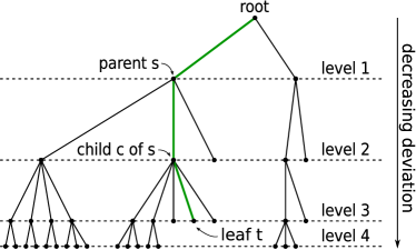
Figure 1: Example of a 4-leveled tree graph which represents an LOCC measurement with at most 4 steps. The branch $B(t)$ (thick green) connects the leaf $t$ with the root node and hence consists of the root node, node $s$ and its child $c$ and the leaf $t$.

In general, a finite LOCC protocol consists of a certain number of steps, where in each step a particular party applies a family $(\Lambda_{k})$ of local quantum operations $\Lambda_{k}\colon\rho\mapsto A_{k}\rho A_{k}^{\dagger}$ with $\Lambda=\sum_{k}\Lambda_{k}$ trace preserving. These quantum operations depend on the course of the protocol so far and the measurement result $k$ is always communicated to all parties. This situation can be depicted by a tree graph (cf. Fig. 1), where the children of each node correspond to a particular operation $\Lambda_{k}$, a level in the tree represents a particular protocol step, and each branch corresponds to a particular course of the protocol.

Hence, a finite LOCC protocol can be represented by a tree graph with root element, where to each node $s$ of the tree, an operator $A_{(s)}$ is associated. (The associated operator for the root node is the identity operator.) For each node, the associated child operators $(A_{(c)})$ shall form a family of Kraus operators of a local CPTP map, i.e., all operators in $(A_{(c)})$ act only non-trivially on some particular party. Then for any path $P$ in this tree we associate an operator $A_{P}$ as the product of the operators in reversed ordering: If $P=(s_{1},\dotsc,s_{m})$, where $s_{k}$ is the parent of $s_{k+1}$, then $A_{P}=A_{(s_{m})}\cdots A_{(s_{1})}$. Note that $A_{P}$ is a product operator. For a node $s$ we then denote by $B(s)$ the path connecting the root element with $s$ (including the root element and $s$).

Figure 2: Introduction of a pseudo-weak measurement and recovery step. Assume that $d({\mathfrak{I}}|A_{B(1)})\leq d({\mathfrak{I}}|A_{B(2)})<\delta$, while $\delta\leq d({\mathfrak{I}}|A_{B(3)})\leq d({\mathfrak{I}}|A_{B(4)})$ in the original situation (a). In (b) the pseudo-weak measurement was introduced with $b_{(1)}$ and $b_{(2)}$ such that $d({\mathfrak{I}}|A_{B(\tilde{1})})=d({\mathfrak{I}}|A_{B(\tilde{2})})=\delta$ (thick green), while the operators at nodes $3$ and $4$ remain —up to a prefactor— unchanged. Then for the nodes $\tilde{1}$ and $\tilde{2}$ a recovery step is introduced (thin red), such that —up to a prefactor— in effect the original operators from the nodes $1$ to $4$ occur. Finally the according parts of the original protocol are added to the outcomes of the recovery measurements (dashed gray).

For an arbitrary $\delta$ with $0<\delta<d({\mathfrak{I}})$ (again, ${\mathfrak{I}}\colon X\mapsto\operatorname{tr}[X]$) we modify the protocol in an iterative procedure as follows (cf. Fig. 2). For any node $s$ we denote by $D_{\delta}(s)$ the set of child nodes for which the deviation dropped below $\delta$, i.e.,

$$D_{\delta}(s)=\{\text{$c$ is child of $s$}\mid d({\mathfrak{I}}|A_{B(c)})<\delta\}.$$ (7)

Let $s$ be a node with non-empty set $D_{\delta}(s)$ but $d({\mathfrak{I}}|A_{B(a)})>\delta$ for any $a\in B(s)$. For such a node, the associated child operators $(A_{(c)})$ are replaced by the pseudo-weak implementation $(A^{\mathrm{pw}}_{(c)})$ with the parameters $(b_{(c)})$ (cf. Sec. III.1) chosen such that $d({\mathfrak{I}}|A^{\mathrm{pw}}_{(c)}A_{B(s)})=\delta$ for all $c\in D_{\delta}(s)$ and $b_{(c)}=0$ else. This is always possible, since regular deviation measures are continuous and the pseudo-weak measurement smoothly interpolates between $A_{(c)}\equiv V_{(c)}\sqrt{A^{\dagger}_{(c)}A_{(c)}}$ and $V_{(c)}$ for $b_{(c)}=0\dotsc\infty$. For the nodes in $D_{\delta}(s)$ we add the recovery step as an additional level (the recovery measurement for the remaining child nodes would be trivial). After the recovery measurement, the according part of the original protocol is appended.

This procedure is repeated, until for all nodes $s$ either $D_{\delta}(s)$ is empty or there exists an $a\in B(s)$ with $d({\mathfrak{I}}|A_{B(a)})=\delta$. It is important to note, that this procedure terminates after a finite number of steps. This is the case, since the number of candidates subject to modification decreases in each step of the procedure; the recovery levels are only introduced when $d({\mathfrak{I}}|A_{B(s)})=\delta$.

We denote by stage I of the protocol the part that does not enter the recovery steps, but rather terminates as soon as $d({\mathfrak{I}}|A_{B(s)})=\delta$ in the modified protocol.

III.3 Analysis of the best-case deviation

For the moment we only consider stage I of the modified protocol (with parameter $\delta$). As an abbreviation we define for each leaf $k$ of this stage the shorthand $A_{k}:=A_{B(k)}$. Let us now define the set

$$S_{\delta}=\{\text{$k$ is leaf}\mid d({\mathfrak{I}}|A_{k})=\delta\}.$$ (8)

Due to our modification of the protocol, $k\notin S_{\delta}$ only if $k$ was already a leaf in the original protocol with $d({\mathfrak{I}}|A_{k})>\delta$.

For each leaf $k$ we let ${\mathfrak{E}}_{k}$ be the continuation of stage I of the modified protocol. With $\Pi$ being the post-processing that “forgets” all results of any pseudo-weak measurement introduced by the protocol splitting (this are those results with parameter $b_{(c)}>0$), the measurement

$$\textstyle{\mathfrak{E}}\colon\rho\mapsto\Pi[\bigoplus_{k}{\mathfrak{E}}_{k}(A_{k}\rho A_{k}^{\dagger})]$$ (9)

is equivalent to the original protocol. Hence, due to property (ii) and (iii) of regular measures $d$, we have

$$d({\mathfrak{E}})\geq\min_{k}d({\mathfrak{E}}_{k}|A_{k})\geq\min[\delta,\min_{k\in S_{\delta}}d({\mathfrak{E}}_{k}|A_{k})].$$ (10)

We now consider the case of $\hat{d}=0$, i.e., for any $\varepsilon>0$ there exists a protocol ${\mathfrak{E}}^{\varepsilon}$ with $d({\mathfrak{E}}^{\varepsilon})<\varepsilon$. Then for any $\delta$ with $0<\delta<d({\mathfrak{I}})$ and any $\varepsilon$ with $0<\varepsilon<\delta$ we have

$$\varepsilon>d({\mathfrak{E}}^{\varepsilon})\geq\min_{k\in S_{\delta}}d({\mathfrak{E}}_{k}|A_{k}).$$ (11)

(Note that ${\mathfrak{E}}_{k}$ and $A_{k}$ depend on $\delta$ and ${\mathfrak{E}}^{\varepsilon}$.) The right-hand side of this inequality can be further lower bounded by

$$y_{\delta}=\inf\{d(\mathfrak{G}|\sqrt{E})\mid\text{$\mathfrak{G}$ is a finite LOCC}\\ \text{measurement, }E\in M_{\delta}\},$$ (12a)

where

$$\mathcal{M}_{\delta}=\{E\text{ is a product operator}\mid E\geq 0,\\ {\textstyle\sum_{\mu}}\operatorname{tr}(\gamma_{\mu}E)=1\text{, and }d({\mathfrak{I}}|\sqrt{E})=\delta\}.$$ (12b)

This is a lower bound, since any ${\mathfrak{E}}_{k}$ is a finite LOCC measurement, $A_{k}^{\dagger}A_{k}/p_{A_{k}}\in\mathcal{M}_{\delta}$ [cf. Eq. (4); the case $p_{A_{k}}=0$ cannot occur due to $\delta<d({\mathfrak{I}})$], and due to property (ia) of regular deviation measures. We have an intermediate result:

$$\hat{d}=0 y_{\delta}=0 0<\delta<d({\mathfrak{I}})$$ only if for any . (13)

The main use of this result is the reverse statement, where $y_{\delta}>0$ for some $\delta$ shows that $\hat{d}>0$. In this case we are not interested in the actual value of $y_{\delta}$, and we therefore now aim to eliminate the infimum in the expression for $y_{\delta}$.

III.4 Specialization to $d_{\mathrm{mf}}$

The special property of the measure $d_{\mathrm{mf}}$, as defined in Eq. (2), we are about to exploit is, that for the discrimination of $N$ states, it is never advantageous to choose a measurement with more than $N$ outcomes (for more than $N$ outcomes one could always combine the results for which $\max_{\nu}p_{\nu}\mathfrak{E}(\rho_{\nu})_{k}$ is achieved at $\mu=\nu$). Therefore, in order to make the set of measurements in the definition of $y_{\delta}$ [cf. Eq. (12a)] a compact set, we extend the allowed measurements to arbitrary global measurements , but at the same time consider only measurements with at most $N$ outcomes.

We also assume that the kernels of the states $(\gamma_{\mu})$ do not share a product vector, i.e., $\bigcap_{\mu}\ker\gamma_{\mu}$ contains no product vector (except $0$). Let $E\in\mathcal{M}_{\delta}$, as defined in Eq. (12b), have the spectral decomposition $E=\sum_{j}e_{j}{{\lvert{j}\rangle}\!{\langle{j}\rvert}}$, where ${\lvert{j}\rangle}$ are product vectors. Then with $R=\sum_{\mu}\gamma_{\mu}$ we have

$$1=\operatorname{tr}(RE)\geq\min_{j}({\langle{j}\rvert}R{\lvert{j}\rangle})\max_{j}e_{j}\geq\eta_{R}\max_{j}e_{j}.$$ (14)

where $\eta_{R}=\inf{\langle{\xi}\rvert}R{\lvert{\xi}\rangle}$, with the infimum taken over all product vectors ${\lvert{\xi}\rangle}$. Since the kernel of $R$ contains no product vector, $\eta_{R}>0$ and hence $e_{j}\leq 1/\eta_{R}$. This in turn shows that we can replace the condition $E\geq 0$ by the compact condition $\openone/\eta_{R}\geq E\geq 0$. Due to the condition $\sum_{\mu}\operatorname{tr}\gamma_{\mu}E=1$, we have $d({\mathfrak{I}}|\sqrt{E})=d[{\mathfrak{I}};(\sqrt{E}\gamma_{\mu}\sqrt{E})]$ which shows due to the continuity of $d$, that the condition $d({\mathfrak{I}}|\sqrt{E})=\delta$ defines a compact set. Hence $\mathcal{M}_{\delta}$ as defined in Eq. (12b) itself is a compact set.

Together with the continuity of regular measures, it follows that $\hat{d}_{\mathrm{mf}}=0$ only if there exists an operator $E$ in $\mathcal{M}_{\delta}$ and a measurement $\mathfrak{G}$ with $d(\mathfrak{G}|\sqrt{E})=0$. Hence the states $(\sqrt{E}\gamma_{\mu}\sqrt{E})$ can be perfectly discriminated and thus are mutually orthogonal, i.e. $\operatorname{tr}(\gamma_{\mu}E\gamma_{\nu}E)=0$ for $\mu\neq\nu$.

Finally, our argument is independent of the a priori probabilities $p_{\mu}>0$, and we hence can choose them to be all equal (this maximizes $d_{\mathrm{mf}}({\mathfrak{I}})$ to $1/N$ and hence the range of $\delta$). The boundary cases $\delta=0$ and $\delta=d_{\mathrm{mf}}({\mathfrak{I}})$ are trivial to fulfill. Letting $\chi=1-\delta$, we arrive at our main result:

Proposition 1.

Let $(\rho_{\mu})$ be a family of $N$ states, such that $\bigcap_{\mu}\ker\rho_{\mu}$ contains no product vector (except 0).

Then $(\rho_{\mu})$ can be discriminated perfectly by asymptotic LOCC, $\hat{d}_{\mathrm{mf}}=0$, only if for all $\chi$ with $1/N\leq\chi\leq 1$ there exists a product operator $E\geq 0$ obeying $\sum_{\mu}\operatorname{tr}(E\rho_{\mu})=1$, $\max_{\mu}\operatorname{tr}(E\rho_{\mu})=\chi$, and $\operatorname{tr}(E\rho_{\mu}E\rho_{\nu})=0$ for $\mu\neq\nu$.

This necessary condition does not imply perfect discrimination for finite LOCC, as we will demonstrate in Section IV.2. We mention, that the Proposition basically holds for any regular deviation measure $d$, for which the optimal general measurement strategy for $N$ arbitrary states can be achieved using at most a certain fixed number of effects.

Note, that the precondition in Proposition 1 is not robust under trivial local embeddings: If a local Hilbert space ${\mathcal{H}}^{(s)}$ is extended to ${\mathcal{H}}^{(s)}\oplus{\mathcal{H}}^{\prime}$, this condition will be violated. However, if $E^{\prime}\in\mathcal{M}_{\delta}$, then the projection onto the original space $E^{\prime}\mapsto E$ is still in $\mathcal{M}_{\delta}$ and $d(\mathfrak{G}|\sqrt{E})=d(\mathfrak{G}|\sqrt{E^{\prime}})$. Therefore, in the Proposition the embedding Hilbert space ${\mathcal{H}}=\bigotimes_{r}{\mathcal{H}}^{(r)}$ should be chosen as small as possible.

IV Examples

IV.1 Product bases

Let $({\lvert{\psi_{\mu}}\rangle})$ be an orthonormal product basis of an $N$-dimensional Hilbert space ${\mathcal{H}}=\bigotimes_{r}{\mathcal{H}}^{(r)}$. We assume that the states $({{\lvert{\psi_{\mu}}\rangle}\!{\langle{\psi_{\mu}}\rvert}})$ can be discriminated by asymptotic LOCC and hence for any $\chi$ with $1/N\leq\chi\leq 1$ there exists an operator $E$ obeying the conditions in Proposition 1. For $1/N<\chi<1/(N-1)$, this operator $E$ must be of full rank, but cannot be a multiple of the identity operator.

We choose some decompositions ${\lvert{\psi_{\mu}}\rangle}=\bigotimes_{r}{\lvert{\omega_{\mu}^{(r)}}\rangle}$ and $E=\bigotimes_{r}E^{(r)}$ with $E^{(r)}\geq 0$. Since ${\langle{\psi_{\nu}}\rvert}E{\lvert{\psi_{\mu}}\rangle}=0$ if and only if $\mu\neq\nu$, it follows that $E{\lvert{\psi_{\mu}}\rangle}=f_{\mu}{\lvert{\psi_{\mu}}\rangle}$ with $f_{\mu}>0$. Hence for any $r$ we have $E^{(r)}{\lvert{\omega_{\mu}^{(r)}}\rangle}=f_{\mu}^{(r)}{\lvert{\omega_{\mu}^{(r)}}\rangle}$ with $f_{\mu}^{(r)}>0$. It follows that a local measurement of the observable $E^{(r)}$ does not change any of the input states. Since for some subsystem $s$, the observable $E^{(s)}$ is not proportional to the identity operator, the measurement of $E^{(s)}$ separates the set of states in at least two non-empty subsets. Each of the subsets is again an orthonormal product basis of a subspace of ${\mathcal{H}}$ and each of the subsets inherits the property that it can be discriminated by asymptotic LOCC. By induction we arrive at

Proposition 2.

If a complete (product) basis can be discriminated perfectly by asymptotic LOCC ($\hat{d}_{\mathrm{mf}}=0$) then it can already be discriminated perfectly by a finite LOCC measurement.

Since $\hat{d}_{\mathrm{mf}}>0$ implies $\hat{d}_{\mathrm{ce}}>0$ [cf. Eqns. (2) and (3)], this Proposition in particular yields an analytical proof of the result of Bennett et al. in Ref. Bennett et al. (1999). Unfortunately, it is not straightforward to extend this type of argument to the situation of an unextendible product basis (then ${\lvert{\psi_{\mu}}\rangle}$ is not necessarily an eigenstate of $E$.).

Remark. In Ref. De Rinaldis (2004) a proof was given that unextendible product bases cannot be discriminated by asymptotic LOCC. (Since a complete basis is also unextendible, this includes Proposition 2 as a special case.) While the statement is likely to hold, the proof given there is incomplete. In particular we question the argument below Eq. (16), showing that the quotient “$M_{N}/c_{N}$” converges to a constant for “$N\rightarrow\infty$” (in this expression $N$ denotes the number of steps until the protocol is aborted). The argument for this convergence is quite general and should hold whenever finite discrimination is not possible (more precisely, if any local measurement either destroys orthogonality or is trivial). For the example in Sec. IV.2, however, the quotient would diverge, since “$c_{N}$” is zero in this case.

IV.2 When Proposition 1 does not decide

The previous example showed that for a wide class of examples, asymptotic LOCC does not provide an advantage over LOCC with finite resources. In this section we give an explicit example for which Proposition 1 does not help to decide whether perfect discrimination via asymptotic LOCC can be performed.

We aim to discriminate the following three mutually orthogonal states on a two-qubit system:

$$\begin{split}{\lvert{\psi_{1}}\rangle}&={\lvert{00}\rangle},\\ {\lvert{\psi_{2}}\rangle}&\propto 2{\lvert{01}\rangle}-(\sqrt{3}+1){\lvert{10}\rangle}-\sqrt{6}\sqrt[4]{3}{\lvert{11}\rangle},\\ {\lvert{\psi_{3}}\rangle}&\propto 2{\lvert{01}\rangle}-(\sqrt{3}-1){\lvert{10}\rangle}+\sqrt{2}\sqrt[4]{3}{\lvert{11}\rangle}.\end{split}$$ (15)

In Ref. Duan et al. (2009), Example 1 , it has been demonstrated, that this set of vectors can be discriminated perfectly by stochastic LOCC, while there exists no perfect discrimination strategy for LOCC in a finite number of steps. In fact, a local effect that does not destroy orthogonality is necessarily proportional to the identity operator.

The only state that is orthogonal to all ${\lvert{\psi_{\mu}}\rangle}$ is entangled and hence we can apply Proposition 1. However, in the Appendix we construct an operator $E_{\chi}$ for $\frac{1}{3}\leq\chi\leq 1$, which satisfies the conditions from Proposition 1. Hence our necessary condition for perfect discrimination by asymptotic LOCC is satisfied, but Proposition 1 does not provide a sufficient criterion.

V Conclusions

We considered the case of asymptotic local operations and classical communication for the discrimination of mutually orthogonal states and derived a necessary condition for perfect asymptotic discrimination to be possible. Our analysis yielded a general necessary condition, cf. Proposition 1, which consists of the existence of a certain product operator. As an example we showed, that any complete basis of product states can be discriminated perfectly by asymptotic LOCC if and only if they can already be discriminated in a finite number of rounds (cf. Proposition 2).

Our result allows to relatively easily exclude whether a family of states can be discriminated by asymptotic LOCC, however it is still unclear whether infinite resources can be of any advantage. Although the general intuition might be, that for perfect discrimination the asymptotic case is not superior, we identified an example, which could be a counter-example for this case as our necessary condition is fulfilled. However, as a sufficient criterion is not available, this question remains open.

*

Appendix A Construction of $E_{\chi}$

In this Appendix we provide an operator $E_{\chi}$ for the states defined in Eq. (15). This operator satisfies the conditions from Proposition 1. We first define the local qubit-operator $A_{\chi}$ via

$$\begin{split}{\langle{0}\rvert}A_{\chi}{\lvert{0}\rangle}&=-(12\sqrt{3}-21)\chi+3\sqrt{3}-3,\\ {\langle{1}\rvert}A_{\chi}{\lvert{1}\rangle}&=(6\sqrt{3}-12)\chi-2\sqrt{3}+6,\\ {\langle{0}\rvert}A_{\chi}{\lvert{1}\rangle}&=\textstyle\sqrt{2\sqrt{3}-3}[(5\sqrt{3}-3)\chi-2\sqrt{3}],\\ {\langle{1}\rvert}A_{\chi}{\lvert{0}\rangle}&={\langle{0}\rvert}A_{\chi}{\lvert{1}\rangle}^{*},\end{split}$$ (16)

and the diagonal operators $B_{\chi}$ and $C_{\chi}$ via

$$\begin{split}{\langle{0}\rvert}B_{\chi}{\lvert{0}\rangle}&=20\chi+2\tilde{\chi}-4,\\ {\langle{1}\rvert}B_{\chi}{\lvert{1}\rangle}&=(12-\sqrt{3})\chi+\tilde{\chi}+\sqrt{3}-1,\end{split}$$ (17)

and

$$\begin{split}{\langle{0}\rvert}C_{\chi}{\lvert{0}\rangle}&=-(4+3\sqrt{3})\chi-\tilde{\chi}+3\sqrt{3}+5,\\ {\langle{1}\rvert}C_{\chi}{\lvert{1}\rangle}&={\langle{1}\rvert}B_{\chi}{\lvert{1}\rangle},\end{split}$$ (18)

where

$$\tilde{\chi}=\sqrt{(115-8\sqrt{3})\chi^{2}-(46-10\sqrt{3})\chi-2\sqrt{3}+4}.$$ (19)

Then with

$$\tilde{E}_{\chi}=\begin{cases}B_{\chi}\otimes C_{\chi}&\text{if $\chi<1/2$}\\ A_{\chi}\otimes{{\lvert{1}\rangle}\!{\langle{1}\rvert}}&\text{else.}\end{cases}$$ (20)

we finally let $E_{\chi}=\tilde{E}_{\chi}/\sum_{\mu}{\langle{\psi_{\mu}}\rvert}\tilde{E}_{\chi}{\lvert{\psi_{\mu}}\rangle}$. One readily verifies that $E_{\chi}$ has the desired properties.

References

- Horodecki et al. (2009) R. Horodecki, P. Horodecki, M. Horodecki, and K. Horodecki, Rev. Mod. Phys. 81, 865 (2009).
- Gühne and Tóth (2009) O. Gühne and G. Tóth, Phys. Rep. 474, 1 (2009).
- Ghosh et al. (2001) S. Ghosh, G. Kar, A. Roy, A. Sen(De), and U. Sen, Phys. Rev. Lett. 87, 277902 (2001).
- Terhal et al. (2001) B. M. Terhal, D. P. DiVincenzo, and D. W. Leung, Phys. Rev. Lett. 86, 5807 (2001).
- Horodecki et al. (2003) M. Horodecki, A. Sen(De), U. Sen, and K. Horodecki, Phys. Rev. Lett. 90, 047902 (2003).
- Ghosh et al. (2004) S. Ghosh, G. Kar, A. Roy, and D. Sarkar, Phys. Rev. A 70, 022304 (2004).
- Chen and Yang (2001) Y.-X. Chen and D. Yang, Phys. Rev. A 64, 064303 (2001).
- Chen and Li (2003) P.-X. Chen and C.-Z. Li, Phys. Rev. A 68, 062107 (2003).
- Chen and Li (2004) P.-X. Chen and C.-Z. Li, Phys. Rev. A 70, 022306 (2004).
- Nathanson (2005) M. Nathanson, J. Math. Phys. 46, 062103 (2005).
- Watrous (2005) J. Watrous, Phys. Rev. Lett. 95, 080505 (2005).
- Duan et al. (2010) R. Duan, Y. Xin, and M. Ying, Phys. Rev. A 81, 032329 (2010).
- Walgate et al. (2000) J. Walgate, A. J. Short, L. Hardy, and V. Vedral, Phys. Rev. Lett. 85, 4972 (2000).
- Bennett et al. (1999) C. H. Bennett, D. P. DiVincenzo, C. A. Fuchs, T. Mor, E. Rains, P. W. Shor, J. A. Smolin, and W. K. Wootters, Phys. Rev. A 59, 1070 (1999).
- Renninger (1960) M. Renninger, Z. f. Phys. A 158, 417 (1960).
- Dicke (1981) R. H. Dicke, Am. J. Phys. 49, 925 (1981).
- De Rinaldis (2004) S. De Rinaldis, Phys. Rev. A 70, 022309 (2004).
- Note (1) A stochastic LOCC measurement is a measurement that can be implemented by means of LOCC with a certain probability , while with probability the measurement will fail. Stochastic LOCC measurements are exactly those with separable effects as in Eq. (1\@@italiccorr) and hence the alternative name separable measurements has also been used.
- Duan et al. (2009) R. Duan, Y. Feng, Y. Xin, and M. Ying, IEEE Trans. Inform. Th. 55, 1320 (2009).
- Barnum et al. (1998) H. Barnum, M. A. Nielsen, and B. Schumacher, Phys. Rev. A 57, 4153 (1998).
- Note (2) In order to see this, note that for any probability distribution we have for any base .
- Note (3) A classical post-processing can be described by a stochastic matrix with , such that .
- Note (4) Using global measurements yields a rather rough estimate. One could also choose the set of fully separable measurements as defined in Eq. (1\@@italiccorr). Then Proposition 1 would contain the additional restriction, that the states must allow a discrimination by separable measurements after result . This condition, however, is difficult to evaluate and hence we only cover the simpler case of global measurements here.
- Note (5) We chose , , and and different local bases.