SIMPLICIAL FLAT NORM WITH SCALE

Abstract

We study the multiscale simplicial flat norm (MSFN) problem, which computes flat norm at various scales of sets defined as oriented subcomplexes of finite simplicial complexes in arbitrary dimensions. We show that the multiscale simplicial flat norm is NP-complete when homology is defined over integers. We cast the multiscale simplicial flat norm as an instance of integer linear optimization. Following recent results on related problems, the multiscale simplicial flat norm integer program can be solved in polynomial time by solving its linear programming relaxation, when the simplicial complex satisfies a simple topological condition (absence of relative torsion). Our most significant contribution is the simplicial deformation theorem, which states that one may approximate a general current with a simplicial current while bounding the expansion of its mass. We present explicit bounds on the quality of this approximation, which indicate that the simplicial current gets closer to the original current as we make the simplicial complex finer. The multiscale simplicial flat norm opens up the possibilities of using flat norm to denoise or extract scale information of large data sets in arbitrary dimensions. On the other hand, it allows one to employ the large body of algorithmic results on simplicial complexes to address more general problems related to currents.

1 Introduction

Currents are standard objects studied in geometric measure theory, and are named so by analogy with electrical currents that have a kind of magnitude and direction at every point. Intuitively, one could think of currents as generalized surfaces with orientations and multiplicities. The mathematical machinery of currents has been used to tackle many fundamental questions in geometric analysis, such as the ones related to area minimizing surfaces, isoperimetric problems, and soap-bubble conjectures [18].

To formally define $d$-currents in ${\mathbb{R}}^{n}$, we first let $\mathcal{D}^{d}$ be the set of $C^{\infty}$ differentiable $d$-forms with compact support. Then the set of $d$-currents is given by the dual space of $\mathcal{D}^{d}$ (denoted $\mathcal{D}_{d}$) with the weak topology. We denote by $\mathcal{R}_{m}$ the set of rectifiable currents, which contains all currents that represent oriented rectifiable sets (i.e., sets which are almost everywhere the countable union of images of Lipschitz maps from ${\mathbb{R}}^{m}$ to ${\mathbb{R}}^{n}$) with integer multiplicities and finite total mass (with multiplicities).

The mass $\operatorname{M}(T)$ of a $d$-dimensional current $T$ can be thought of intuitively as the weighted $d$-dimensional volume of the generalized object represented by $T$. For instance, the mass of a $2$-dimensional current can be taken as the area of the surface it represents. Formally, the mass of $T$ is given by $M(T)=\sup_{\phi\in\mathcal{D}^{d}}\{T(\phi)\mid\sup\|\phi(x)\|\leq 1\}.$

The boundary $\partial T$ of a current $T$ is defined by duality with forms. That is, we have $\partial T(\phi)=T(d\phi)$ for every differential form $\phi\in\mathcal{D}^{d}$. Note that when $T$ represents a smooth oriented manifold with boundary, this corresponds to the usual definition of boundary. We restrict our attention to integral currents $T$ that are rectifiable currents with a rectifiable boundary (i.e., $T\in\mathcal{R}_{m}$ and $\partial T\in\mathcal{R}_{m-1}$). The flat norm of a $d$-dimensional current $T$ is given by

$${\mathbb{F}}(T)=\min_{S}\{\operatorname{M}(T-\partial S)+\operatorname{M}(S)~{}\big{|}~{}T-\partial S\in{\mathscr{E}}_{d},\,S\in{\mathscr{E}}_{d+1}\},$$ (1)

where ${\mathscr{E}}_{d}$ is the set of $d$-dimensional currents with compact support. One also uses flat norm to measure the “distance” between two $d$-currents. More precisely, the flat norm distance between two $d$-currents $T$ and $P$ is given by

$${\mathbb{F}}(T,P)=\inf\{\operatorname{M}(Q)+\operatorname{M}(R)\,\big{|}\,T-P=Q+\partial R,\,Q\in{\mathscr{E}}_{d},\,R\in{\mathscr{E}}_{d+1}\}.$$ (2)

Morgan and Vixie [19] showed that the $L^{1}$ total variation functional ($L^{1}$TV) introduced by Chan and Esedoḡlu [3] computes the flat norm for boundaries $T$ with integer multiplicity. Given this correspondence, and the use of scale in $L^{1}$TV, Morgan and Vixie defined [19] the flat norm with scale $\lambda\in[0,\infty)$ of an oriented $d$-dimensional set $T$ as

$${\mathbb{F}}_{\lambda}(T)\equiv\min_{S}\{\operatorname{V}_{d}(T-\partial S)+\lambda\operatorname{V}_{d+1}(S)\},$$ (3)

where $S$ varies over oriented $(d+1)$-dimensional sets, and $\operatorname{V}_{d}$ is the $d$-dimensional volume, used in place of mass. Figure 1 illustrates this definition. Flat norm of the 1D current $T$ is given by the sum of the length of the resulting oriented curve $T-\partial S$ (shown separated from the input curve for clarity) and the area of the 2D patch $S$ shown in red. Large values of $\lambda$, above the curvature of both humps in the curve $T$, preserve both humps. Values of $\lambda$ between the two curvatures eliminate the hump on the right. Even smaller values “smooth out” both humps as illustrated here, giving a more “flat” curve, as $S$ can now be comprised of much bigger 2D patches.

Figure 1: 1D current $T$, and flat norm decomposition $T-\partial S$ at appropriate scale $\lambda$. The resulting current is shown slightly separated from the input current for clearer visualization.

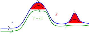
Figure 1 illustrates the utility of flat norm for deblurring or smoothing applications, e.g., in 3D terrain maps or 3D image denoising. But efficient methods for computing flat norm are known only for certain types of currents in two dimensions. For $d=1$, Under the setting where $T$ is a boundary, i.e., a loop, embedded in ${\mathbb{R}}^{2}$ and the minimizing surface $S\in{\mathbb{R}}^{2}$ as well, the flat norm could be calculated efficiently, for instance, using graph cut methods [16] – see the work of Goldfarb and Yin [14] and Vixie et al. [29], and references therein. Motivated by applications in image analysis, these approaches usually worked with a grid representation of the underlying space (${\mathbb{R}}^{2}$). Pixels in the image readily provide such a representation.

While it is computationally convenient that $L^{1}$TV minimizers give us the scaled flat norm for the input images, this approach restricts us to currents that are boundaries of codimension 1. Correspondingly, the calculation of flat norm for $1$-boundaries embedded in higher dimensional spaces, e.g., ${\mathbb{R}}^{3}$, or for input curves that are not necessarily boundaries has not received much attention so far. Similarly, flat norm calculations for higher dimensional input sets have also not been well-studied. Such situations often appear in practice – for instance, consider the case of an input set $T$ that is a curve sitting on a manifold embedded in ${\mathbb{R}}^{3}$, with choices for $S$ restricted to this manifold as well. Further, computational complexity of calculating flat norm in arbitrary dimensions has not been studied. But this is not a surprising observation, given the continuous, rather than combinatorial, setting in which flat norm computation has been posed so far.

Simplicial complexes that triangulate the input space are often used as representations of manifolds. Such representations use triangular or tetrahedral meshes [11] as opposed to the uniform square or cubical grid meshes in ${\mathbb{R}}^{2}$ and ${\mathbb{R}}^{3}$. Various simplicial complexes are often used to represent data (in any dimension) that captures interactions in a broad sense, e.g., the Vietoris–Rips complex to capture coverage of coordinate-free sensor networks [6, 7]. It is natural to consider flat norm calculations in such settings of simplicial complexes for denoising or regularizing sets, or for other similar tasks. At the same time, requiring that the simplicial complex be embedded in high dimensional space modeled by regular square grids may be cumbersome, and computationally prohibitive in many cases.

1.1 Our Contributions

We define a simplicial flat norm (SFN) for an input set $T$ given as a subcomplex of the finite oriented simplicial complex $K$ triangulating the set, or underlying space $\Omega$. More generally, $T$ is the simplicial representation of a rectifiable current with integer multiplicities. The choices of the higher dimensional sets $S$ are restricted to $K$ as well. We extend this definition to the multiscale simplicial flat norm (MSFN) by including a scale parameter $\lambda$. The simplicial flat norm is thus a special case of the multiscale simplicial flat norm with the default value of $\lambda=1$.

This discrete setting lets us address the worst case complexity of computing flat norm. Given its combinatorial nature, one would expect the problem to be difficult in arbitrary dimensions. Indeed, we show the problem of computing the multiscale simplicial flat norm is NP-complete by reducing the optimal bounding chain problem (OBCP), which was recently shown to be NP-complete [10], to a special case of the multiscale simplicial flat norm problem. We cast the problem of finding the optimal $S$, and thus calculating the multiscale simplicial flat norm, as an integer linear programming (ILP) problem. Given that the original problem is NP-complete, instances of this ILP could be hard to solve. Utilizing recent work [8] on the related optimal homologous chain problem (OHCP), we provide conditions on $K$ under which this ILP problem can in fact be solved in polynomial time. In particular, the multiscale simplicial flat norm can be computed in polynomial time when $T$ is $d$-dimensional, and $K$ is $(d+1)$-dimensional and orientable, for all $d\geq 0$. A similar result holds for the case when $T$ is $d$-dimensional, and $K$ is $(d+1)$-dimensional and embedded in ${\mathbb{R}}^{d+1}$, for all $d\geq 0$.

Our most significant contribution is the simplicial deformation theorem (Theorem 5.1), which states that given an arbitrary $d$-current in $\lvert K\rvert$ (underlying space), we are assured of an approximating current in the $d$-skeleton of $K$. This result is a substantial modification and generalization of the classical deformation theorem for currents on to square grids. Our deformation theorem explicitly specifies the dependence of the bounds of approximation on the regularity and size of the simplices in the simplicial complex. Hence it is immediate from the theorem that as we refine the simplicial complex $K$ while preserving the bounds on simplicial regularity, the flat norm distance between an arbitrary $d$-current in $\lvert K\rvert$ and its deformation onto the $d$-skeleton of $K$ vanishes. More importantly, such refinement of $K$ does not affect the efficient computability of the multiscale simplicial flat norm by solving the associated ILP in many cases, e.g., when $K$ is orientable or when it is full-dimensional.

1.2 Work on Related Problems

The problem of computing multiscale simplicial flat norm is closely related to two other problems on chains defined on simplicial complexes – the optimal homologous chain problem (OHCP) and the optimal bounding chain problem (OBCP). Given a $d$-chain $\mathbf{t}$ of the simplicial complex $K$, the optimal homologous chain problem is to find a $d$-chain $\mathbf{x}$ that is homologous to $\mathbf{t}$ such that $\lVert\mathbf{x}\rVert_{1}$ is minimal. In the optimal bounding chain problem, we are given a $d$-chain $\mathbf{t}$ of $K$, and the goal is to find a $(d+1)$-chain $\mathbf{s}$ of $K$ whose boundary is $\mathbf{t}$ and $\lVert\mathbf{s}\rVert_{1}$ is minimal. The optimal bounding chain problem is closely related to the problem of finding an area-minimizing surface with a given boundary [18]. Computing the multiscale simplicial flat norm could be viewed, in a simple sense, as combining the objectives of the corresponding optimal homologous chain and optimal bounding chain problem instances, with the scale factor determining the relative importance of one objective over the other.

When $\mathbf{t}$ is a cycle and the homology is defined over ${\mathbb{Z}}_{2}$, Chen and Freedman showed that the optimal homologous chain problem is NP-hard [4]. Dey, Hirani, and Krishnamoorthy [8] studied the original version of the optimal homologous chain problem with homology defined over ${\mathbb{Z}}$, and showed that the problem is in fact solvable in polynomial time when $K$ satisfies certain conditions (when it has no relative torsion). Recently, Dunfield and Hirani [10] have shown that the optimal homologous chain problem with homology defined over ${\mathbb{Z}}$ is NP-complete. We will use their results to show that the problem of computing the multiscale simplicial flat norm is NP-complete (see Section 2.1). These authors also showed that the optimal bounding chain problem with homology defined over ${\mathbb{Z}}$ is NP-complete as well. Their result builds on the previous work of Agol, Hass, and Thurston [1], who showed that the knot genus problem is NP-complete, and a slightly different version of the least area surface problem is NP-hard.

The standard simplicial approximation theorem from algebraic topology describes how continuous maps are approximated by simplicial maps that satisfy the star condition [20, §14]. Our simplicial deformation theorem applies to currents, which are more general objects than continuous maps. More importantly, we present explicit bounds on the expansion of mass of the current resulting from simplicial approximation. In his PhD thesis, Sullivan [26] considered deforming currents on to the boundary of convex sets in a cell complex, which are more general than the simplices we work with. But simplicial complexes admit efficient algorithms more naturally than cell complexes. We adopt a different approach for deformation from Sullivan and obtain new bounds on the approximations (see Section 5.2). Along with the multiscale simplicial flat norm, our deformation theorem also establishes how the optimal homologous chain problem and optimal bounding chain problem could be used on general continuous inputs by taking simplicial approximations, thus expanding widely the applicability of this family of techniques.

2 Definition of Simplicial Flat Norm

Consider a finite $p$-dimensional simplicial complex $K$ triangulating the set $\Omega$, where the simplices are oriented, with $p\geq d+1$. The set $T$ is defined as the integer multiple of an oriented $d$-dimensional subcomplex of $K$, representing a rectifiable $d$-current with integer multiplicity. Let $m$ and $n$ be the number of $d$- and $(d+1)$-dimensional simplices in $K$, respectively. The set $T$ is then represented by the $d$-chain $\sum_{i=1}^{m}t_{i}\sigma_{i}$, where $\sigma_{i}$ are all $d$-simplices in $K$ and $t_{i}$ are the corresponding weights. We will represent this chain by the vector of weights $\mathbf{t}\in{\mathbb{Z}}^{m}$. We use bold lower case letters to denote vectors, and the corresponding letter with subscript to denote components of the vector, e.g., $\mathbf{x}=[x_{j}]$. For $\mathbf{t}$ representing the set $T$ with integer multiplicity of one, $t_{i}\in\{-1,0,1\}$ with $-1$ indicating that the orientations of $\sigma_{i}$ and $T$ are opposite. But $t_{i}$ can take any integer value in general. Thus, $\mathbf{t}$ is the representation of $T$ in the elementary $d$-chain basis of $K$. We consider $(d+1)$-chains in $K$ modeling sets $S$ representing rectifiable $(d+1)$-currents with integer multiplicities, and denote them similarly by $\sum_{j=1}^{n}s_{j}\tau_{j}$ in the elementary $(d+1)$-chain basis of $K$ consisting of the individual simplices $\tau_{j}$. We denote the chain modeling such a set $S$ using the corresponding vector of weights $\mathbf{s}\in{\mathbb{Z}}^{n}$.

Relationships between the $d$- and $(d+1)$-chains of $K$ are captured by its $(d+1)$-boundary matrix $[\partial_{d+1}]$, which is an $m\times n$ matrix with entries in $\{-1,0,1\}$. If the $d$-simplex $\sigma_{i}$ is a face of the $(d+1)$-simplex $\tau_{j}$, then the $(i,j)$ entry of $[\partial_{d+1}]$ is nonzero, otherwise it is zero. This nonzero value is $+1$ if the orientations of $\sigma_{i}$ and $\tau_{j}$ agree, and is $-1$ when their orientations are opposite. The $d$-chain representing the set $T-\partial_{d+1}S$ is then given as

$$\mathbf{x}=\mathbf{t}-[\partial_{d+1}]\mathbf{s}.$$

Notice that $\mathbf{x}\in{\mathbb{Z}}^{m}$. We define the simplicial flat norm (SFN) of $T$ represented by the $d$-chain $\mathbf{t}$ in the $(d+1)$-dimensional simplicial complex $K$ as

$$F_{S}(T)=\min_{\mathbf{s}\in{\mathbb{Z}}^{n}}\left\{\sum_{i=1}^{m}\operatorname{V}_{d}(\sigma_{i})\lvert x_{i}\rvert+\sum_{j=1}^{n}\operatorname{V}_{d+1}(\tau_{j})\lvert s_{j}\rvert~{}\big{|}~{}\mathbf{x}=\mathbf{t}-[\partial_{d+1}]\mathbf{s},\,\mathbf{x}\in{\mathbb{Z}}^{m}\right\}.$$ (4)

Since $\mathbf{x}$ and $\mathbf{s}$ are chains in a simplicial complex, the masses of the currents they represent (as given in Equation 1) are indeed given by the weighted sums of the volumes of the corresponding simplices. The integer restrictions $\mathbf{x}\in{\mathbb{Z}}^{m}$ and $\mathbf{s}\in{\mathbb{Z}}^{n}$ are important in this definition as we are studying currents with integer multiplicities. The simplicial flat norm is intuitively the problem of deforming an input chain to another chain of least cost, where cost is determined both by the mass of the resulting chain and the size of the deformation (constrained to the complex) used to get it. For instance, in a triangulation of a manifold, we constrain ourselves to only use deformations on the manifold. We generalize the definition of SFN to define a multiscale simplicial flat norm (MSFN) of $T$ in the simplicial complex $K$ by including a scale parameter $\lambda\in[0,\infty)$.

$$F^{\lambda}_{S}(T)=\min_{\mathbf{s}\in{\mathbb{Z}}^{n}}\left\{\sum_{i=1}^{m}\operatorname{V}_{d}(\sigma_{i})\lvert x_{i}\rvert+\lambda\left(\sum_{j=1}^{n}\operatorname{V}_{d+1}(\tau_{j})\lvert s_{j}\rvert\right)~{}\big{|}~{}\mathbf{x}=\mathbf{t}-[\partial_{d+1}]\mathbf{s},\,\mathbf{x}\in{\mathbb{Z}}^{m}\right\}.$$ (5)

This definition is the simplicial version of the multiscale flat norm defined in Equation (3). The default, or nonscale, simplicial flat norm in Equation (4) is a special case of the multiscale simplicial flat norm with the default value of $\lambda=1$.

The (non-simplicial) flat norm with scale $\lambda>0$ of a $d$-dimensional current $T$ can be rewritten as ${\mathbb{F}}_{\lambda}(T)=\lambda^{d}\cdot{\mathbb{F}}_{1}(T/\lambda)$. Thus the flat norm with scale can be thought of as the traditional flat norm applied to a scaled copy of the input current. An equivalent statement can be made for the simplicial flat norm, but crucially requires that the simplicial complex be similarly scaled. To avoid this complex scaling issue especially when considering all possible scales, and to simplify our notation, we henceforth study the more general multiscale simplicial flat norm (which also allows us to consider the $\lambda=0$ case).

We assume the $d$- and $(d+1)$-dimensional volumes of simplices to be any nonnegative values. For example, when $\sigma_{i}$ is a $1$-simplex, i.e., edge, $\operatorname{V}_{1}(\sigma_{i})$ could be taken as its Euclidean length. Similarly, $\operatorname{V}_{2}(\tau_{j})$ for a triangle $\tau_{j}$ could be its area. For ease of notation, we denote $\operatorname{V}_{d}(\sigma_{i})$ by $w_{i}$ and $\operatorname{V}_{d+1}(\tau_{j})$ by $v_{j}$, with the dimensions $d$ and $d+1$ evident from the context.

Remark 2.1.

The minimum in the definition of the multiscale simplicial flat norm (Equation 5) indeed exists. The function

$$f^{\lambda}(T,S)=\sum_{i=1}^{m}w_{i}\lvert x_{i}\rvert+\lambda\,(\sum_{j=1}^{n}v_{j}\lvert s_{j}\rvert)~{}~{}\,\mbox{ with }~{}~{}\,\mathbf{x}=\mathbf{t}-[\partial_{d+1}]\mathbf{s}\,$$ (6)

is lower bounded by zero, as it is the sum of nonnegative entries (we have $\lambda\geq 0$). Notice that $F^{\lambda}_{S}(T)=\min_{S}f^{\lambda}(T,S)$. Further, we only consider integral $\mathbf{s}$ defined on the finite simplicial complex $K$, and hence there are only a finite number of values for this function. Hence its minimum indeed exists, which defines the multiscale simplicial flat norm of $\mathbf{t}$. On the other hand, the proof of existence of minimum in the original definition of flat norm for rectifiable currents employs the Hahn–Banach theorem [13, pg. 367].

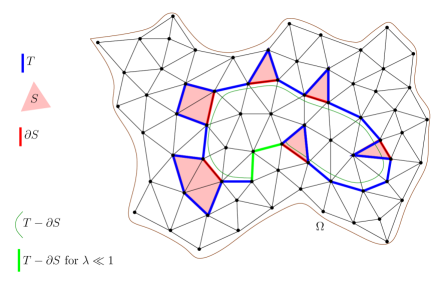
We illustrate the optimal decompositions to compute the multiscale simplicial flat norm for two different scales ($\lambda=1$ and $\lambda\ll 1$) in Figure 2. Notice that the input set $T$, shown in blue, is not a closed loop here. It is a subcomplex of the simplicial complex triangulating $\Omega$. The underlying set $\Omega$ need not be embedded in ${\mathbb{R}}^{2}$ – it could be sitting in ${\mathbb{R}}^{3}$ or any higher dimension. We do not show the orientations of individual simplices and chains so as not to clutter the figure. We could take each triangle to be oriented counterclockwise (CCW), with $T$ oriented CCW as well, and each edge oriented arbitrarily. When scale $\lambda=1$, we get the default SFN of $T$, where the $S$ chosen (shown in light pink) is such that the resulting optimal $T-\partial S$ (indicated by the thin curve in dark green) is devoid of all the “kinks”, but is similar to $T$ in overall form. This removal of the tightest “kinks” is a discrete analogue of how the $\lambda$ in the flat norm relates to the curvature in the continuous case. For $\lambda\ll 1$, the second term in the definition (Equation 5) contributes much less to the multiscale simplicial flat norm. As such, the optimal $T-\partial S$ consists of a short chain of two edges (shown in light green), which closes the original $T$ curve to form a loop. $S$ in this case includes the triangles in the former choice of $S$, and all other triangles enclosed by the original curve $T$ and the resulting $T-\partial S$.

Figure 2: The multiscale simplicial flat norm illustrated for two different scales $\lambda=1$ and $\lambda\ll 1$. See text for explanation.

2.1 Complexity of multiscale simplicial flat norm

To study the complexity of computing the multiscale simplicial flat norm, we consider a decision version of the problem, termed decision-MSFN or DMSFN. The function $f^{\lambda}(T,S)$ used here is defined in Equation 6, with the modification that $w_{i}$ and $v_{j}$ are assumed to be rational for purposes of analyses of complexity.

Definition 2.2 (DMSFN).

Given a $p$-dimensional finite simplicial complex $K$ with $p\geq d+1$, a set $T$ defined as a $d$-subcomplex of $K$, a scale $\lambda\in[0,\infty)$, and a rational number $f_{0}\geq 0$, does there exist a $(d+1)$-dimensional subcomplex $S$ of $K$ such that $f^{\lambda}(T,S)\leq f_{0}$?

The related optimal homologous chain problem (OHCP) was recently shown to be NP-complete [10, Theorem 1.4]. We reduce OHCP to a special case of DMSFN, thus showing that DMSFN is NP-complete as well. The default optimization version of MSFN consequently turns out to be NP-hard.

Theorem 2.3.

DMSFN is NP-complete, and MSFN is NP-hard.

Proof.

DMSFN lies in NP as we can calculate $f^{\lambda}(T,S)$ in polynomial time when given a pair of $d$- and $(d+1)$-chains $\mathbf{t}$ and $\mathbf{s}$, respectively, of the simplicial complex $K$. On the other hand, given an instance of the optimal homologous chain decision problem, we can reduce it to the DMSFN by taking $\lambda=0$ and $w_{i}=1$ for $1\leq i\leq m$. Since the optimal homologous chain problem was recently shown to be NP-complete [10, Theorem 1.4], the result follows. ∎

Remark 2.4.

Although we showed MSFN is NP-hard in general, the case for any particular $\lambda>0$ is not known. For $\lambda$ large enough, the problem in fact becomes easy– when the $(d+1)$-simplices have positive volumes and $\lambda>(\sum w_{i})/\min v_{j}$, then optimality occurs when $\mathbf{s}$ is the empty $(d+1)$-chain.

We now consider attacking the multiscale simplicial flat norm problem using techniques from the area of discrete optimization. Even though the problem is NP-hard, this approach helps us to identify special cases in which we can compute the multiscale simplicial flat norm in polynomial time.

3 Multiscale Simplicial Flat Norm and Integer Linear Programming

The problem of finding the multiscale simplicial flat norm of the $d$-chain $\mathbf{t}$ (Equation 5) can be cast formally as the following optimization problem.

$$\begin{array}[]{ll}\mbox{minimize}&\sum_{i=1}^{m}w_{i}\lvert x_{i}\rvert+\lambda(\sum_{j=1}^{n}v_{j}\lvert s_{j}\rvert)\\ \vspace*{-0.13in}\\ \mbox{subject to}&~{}~{}~{}~{}~{}~{}\mathbf{x}=\mathbf{t}-[\partial_{d+1}]\mathbf{s},\\ &~{}~{}~{}~{}~{}~{}\mathbf{x}\in{\mathbb{Z}}^{m},~{}\mathbf{s}\in{\mathbb{Z}}^{n}.\end{array}$$ (7)

The objective function is piecewise linear in the integer variables $\mathbf{x}$ and $\mathbf{s}$. Using standard modeling techniques from linear optimization [2, pg. 18], we can reformulate the problem as the following integer linear program (ILP).

$$\begin{array}[]{ll}\min&\sum_{i=1}^{m}w_{i}(x^{+}_{i}+x^{-}_{i})\,+\,\lambda\left(\sum_{j=1}^{n}v_{j}(s^{+}_{j}+s^{-}_{j})\right)\\ \vspace*{-0.13in}\\ \mbox{s.t. }&\mathbf{x}^{+}-\mathbf{x}^{-}=\mathbf{t}-[\partial_{d+1}](\mathbf{s}^{+}-\mathbf{s}^{-})\\ &\mathbf{x}^{+},\mathbf{x}^{-}\geq\mathbf{0},~{}~{}\mathbf{s}^{+},\mathbf{s}^{-}\geq\mathbf{0}\\ &\mathbf{x}^{+},\mathbf{x}^{-}\in{\mathbb{Z}}^{m},~{}~{}\mathbf{s}^{+},\mathbf{s}^{-}\in{\mathbb{Z}}^{n}.\end{array}$$ (8)

The objective function coefficients need to be nonnegative for this formulation to work – indeed, we have $w_{i},v_{j}$, and $\lambda$ nonnegative. Integer linear programming is NP-complete [22]. The linear programming relaxation of the ILP above is obtained by ignoring the integer restrictions on the variables.

$$\begin{array}[]{ll}\min&\sum_{i=1}^{m}w_{i}(x^{+}_{i}+x^{-}_{i})\,+\,\lambda\left(\sum_{j=1}^{n}v_{j}(s^{+}_{j}+s^{-}_{j})\right)\\ \vspace*{-0.13in}\\ \mbox{s.t. }&\mathbf{x}^{+}-\mathbf{x}^{-}=\mathbf{t}-[\partial_{d+1}](\mathbf{s}^{+}-\mathbf{s}^{-})\\ &\mathbf{x}^{+},\mathbf{x}^{-}\geq\mathbf{0},~{}~{}\mathbf{s}^{+},\mathbf{s}^{-}\geq\mathbf{0}\end{array}$$ (9)

We are interested in instances of this linear program (LP) that have integer optimal solutions, which hence are optimal solutions for the original ILP (Equation 8) as well. Totally unimodular matrices yield a prime class of linear programming problems with integral solutions. Recall that a matrix is totally unimodular if all its subdeterminants equal $-1,0,$ or $1$; in particular, each entry is $-1,0,$ or $1$. The connection between total unimodularity and linear programming is specified by the following theorem.

Theorem 3.1.

[28] Let $A$ be an $m\times n$ totally unimodular matrix, and $\mathbf{b}\in{\mathbb{Z}}^{m}$. Then the polyhedron ${\cal P}=\{\mathbf{x}\in{\mathbb{R}}^{n}\,|\,A\mathbf{x}=\mathbf{b},\,\mathbf{x}\geq\mathbf{0}\}$ has integral vertices.

Notice that the feasible set of the multiscale simplicial flat norm LP (Equation 9) has the form specified in the theorem above, with the variable vector $(\mathbf{x}^{+},\mathbf{x}^{-},\mathbf{s}^{+},\mathbf{s}^{-})$ in place of $\mathbf{x}$. The corresponding equality constraint matrix $A$ has the form $\begin{bmatrix}I&-I&B&-B\end{bmatrix}$, where $I$ is the identity matrix and $B=[\partial_{d+1}]$. The input $d$-chain $\mathbf{t}$ is in place of the right-hand side vector $\mathbf{b}$. In order to use Theorem 3.1 for computing the multiscale simplicial flat norm, we connect the total unimodularity of constraint matrix $A$ and that of boundary matrix $B$.

Lemma 3.2.

If $B=[\partial_{d+1}]$ is totally unimodular, then so is the matrix $A=\begin{bmatrix}I&-I&B&-B\end{bmatrix}$.

Proof.

Starting with $B$, we get the matrix $A$ by appending columns of $B$ scaled by $-1$ to its right, and appending columns with a single nonzero entry of $\pm 1$ to its left. Both these classes of operations preserve total unimodularity [22, pg. 280]. ∎

Consequently, we get the following result on polynomial time computability of the multiscale simplicial flat norm.

Theorem 3.3.

If the boundary matrix $[\partial_{d+1}]$ of the finite oriented simplicial complex $K$ is totally unimodular, then the multiscale simplicial flat norm of the set $T$ specified as a $d$-chain $\mathbf{t}\in{\mathbb{Z}}^{m}$ of $K$ can be computed in polynomial time.

Proof.

The problem of computing the multiscale simplicial flat norm of $T$ (Equation 5) is cast as the optimization problem given in Equation (7). This problem is reformulated as an instance of ILP (Equation 8). We get the multiscale simplicial flat norm LP (Equation 9) by relaxing the integrality constraints of this ILP. As noted in Remark 2.1, the optimal cost of this LP is finite. The polyhedron of this LP has at least one vertex, given that all variables are nonnegative [2, Cor. 2.2]. By Lemma 3.2, the constraint matrix of this LP is totally unimodular, as $[\partial_{d+1}]$ is so. Hence by Theorem 3.1, all vertices of the feasible region of the multiscale simplicial flat norm LP are integral, since $\mathbf{t}\in{\mathbb{Z}}^{m}$.

An optimal solution $(\mathbf{x}^{+}_{*},\mathbf{x}^{-}_{*},\mathbf{s}^{+}_{*},\mathbf{s}^{-}_{*})$ of the multiscale simplicial flat norm LP can be found in polynomial time using an interior point method [2, Chap. 9]. If it happens to be a unique optimal solution, then it will be a vertex, and hence will be integral by Theorem 3.1. Hence it is an optimal solution to the ILP (Equation 8).

If the optimal solution is not unique, then $(\mathbf{x}^{+}_{*},\mathbf{x}^{-}_{*},\mathbf{s}^{+}_{*},\mathbf{s}^{-}_{*})$ may be nonintegral. But since the optimal cost is finite, there must exist a vertex in its polyhedron that has this minimum cost. Given a nonintegral optimal solution obtained by an interior point method, one can find such an integral optimal solution at a vertex in polynomial time [15]. Hence the multiscale simplicial flat norm ILP can be solved in polynomial time in this case as well. ∎

Remark 3.4.

We point out that since the boundary matrix $B=[\partial_{d+1}]$ has entries only in $\{-1,0,1\}$, the constraint matrix of the multiscale simplicial flat norm LP (Equation 9) also has entries only in $\{-1,0,1\}$. Hence the multiscale simplicial flat norm LP can be solved in strongly polynomial time [27], i.e., the time complexity is independent of the objective function and right-hand side coefficients, and depends only on the dimensions of the problem.

Remark 3.5.

Components of variables $\mathbf{x}^{+},\mathbf{x}^{-},\mathbf{s}^{+},\mathbf{s}^{-}$ in the multiscale simplicial flat norm ILP (Equation 8) could assume values other than $\{-1,0,1\}$, indicating integer multiplicities higher than $1$ for the corresponding simplices in the optimal decomposition. The definition of multiscale simplicial flat norm (Equation 5) does allow such larger multiplicities. At the same time, if one insists on using each $(d+1)$-simplex at most once when calculating the multiscale simplicial flat norm, and insists on similar restrictions on $d$-simplices in the optimal decomposition, we can modify the ILP such that Theorem 3.3 still holds.

Denoting the entire variable vector by $\mathbf{x}=(\mathbf{x}^{+},\mathbf{x}^{-},\mathbf{s}^{+},\mathbf{s}^{-})\in{\mathbb{Z}}^{2m+2n}$, we add the upper bound constraints $\mathbf{x}\leq\mathbf{1}$, where $\mathbf{1}$ is the $(2m+2n)$-vector of ones. These inequalities could be converted to the set of equations $\mathbf{x}+\mathbf{y}=\mathbf{1}$, where $\mathbf{y}$ is the $(2m+2n)$-vector of slack variables that are nonnegative. These modifications give an ILP whose polyhedron is in the same form as described in Theorem 3.1, with the equations denoted as $A^{\prime}\mathbf{x}^{\prime}=\mathbf{b}^{\prime}$ for the variable vector $\mathbf{x}^{\prime}=(\mathbf{x},\mathbf{y})$. The new constraint matrix $A^{\prime}$ is related to the constraint matrix $A$ of the original multiscale simplicial flat norm ILP given in Lemma 3.2 as

$$A^{\prime}=\begin{bmatrix}A&O\\ I&I\end{bmatrix},$$

where $I$ is the $2m+2n$ identity matrix, and $O$ is the $m\times(2m+2n)$ zero matrix. Hence $A^{\prime}$ is obtained from $A$ by first adding $2m+2n$ rows with a single nonzero entry of $+1$, and then adding to the resulting matrix $2n+2m$ more columns with a single nonzero entry of $+1$. These operations preserve total unimodularity [22, pg. 280], and hence the new constraint matrix $A^{\prime}$ is totally unimodular when $[\partial_{d+1}]$ is so. The new right-hand side vector $\mathbf{b}^{\prime}\in{\mathbb{Z}}^{3m+2n}$ consists of the input chain $\mathbf{t}$ and the vector of ones from the new upper bound constraints.

Since the efficient computability of the multiscale simplicial flat norm depends on the total unimodularity of the boundary matrix, we study the conditions under which total unimodularity of boundary matrices can be guaranteed.

4 Simplicial Complexes and Relative Torsion

Dey, Hirani, and Krishnamoorthy [8] have given a simple characterization of the simplicial complex whose boundary matrix is totally unimodular. In short, if the simplicial complex does not have relative torsion then its boundary matrix is totally unimodular. We state this and other related results here for the sake of completeness, and refer the reader to the original paper [8] for details and proofs. The simplicial complex $K$ in these results has dimension $d+1$ or higher. Recall that a $d$-dimensional simplicial complex is pure  if it consists of $d$-simplices and their faces, i.e., there are no lower dimensional simplices that are not part of some $d$-simplex in the complex.

Theorem 4.1.

[8, Theorem 5.2] The boundary matrix $[\partial_{d+1}]$ of a finite simplicial complex $K$ is totally unimodular if and only if $H_{d}(L,L_{0})$ is torsion-free for all pure subcomplexes $L_{0},L$ of $K$, with $L_{0}\subset L$.

These authors further describe situations in which the absence of relative torsion is guaranteed. The following two special cases describe simplicial complexes for which the boundary matrix is always totally unimodular.

Theorem 4.2.

[8, Theorem 4.1] The boundary matrix $[\partial_{d+1}]$ of a finite simplicial complex triangulating a compact orientable $(d+1)$-dimensional manifold is totally unimodular.

Theorem 4.3.

[8, Theorem 5.7] The boundary matrix $[\partial_{d+1}]$ of a finite simplicial complex embedded in ${\mathbb{R}}^{d+1}$ is totally unimodular.

For simplicial complexes of dimension $2$ or lower, the boundary matrix is totally unimodular when the complex does not have a Möbius subcomplex.

Theorem 4.4.

[8, Theorem 5.13] For $d\leq 1$, the boundary matrix $[\partial_{d+1}]$ is totally unimodular if and only if the finite simplicial complex has no $(d+1)$-dimensional Möbius subcomplex.

It is appropriate to mention here that the connection between total unimodularity of boundary matrices and torsion in the complex has been observed as early as in 1895 by Poincaré[21]. However, the result in [8] connecting the total unimodularity with relative torsion is different and has led to a polynomial time algorithm for the OHCP problem. Notice that a complex can be torsion-free, but have non-trivial relative torsion. The Möbius strip is such an example.

We illustrate the implications of the results above for the efficient computation of the multiscale simplicial flat norm by considering certain sets. When the input set $T$ is of dimension 1, and is described on an orientable $2$-manifold to which the choices of $2$-dimensional set $S$ are also restricted, we can always compute its multiscale simplicial flat norm by solving the multiscale simplicial flat norm LP (Equation 9) in polynomial time. A similar result holds when $T$ is a set of dimension $2$ described as a subcomplex of a $3$-complex sitting in ${\mathbb{R}}^{3}$. For a $1$-dimensional set $T$ with choices of $S$ restricted to a $2$-complex $K$, we can always compute the multiscale simplicial flat norm of $T$ efficiently as long as $K$ does not have a $2$-dimensional Möbius subcomplex. Notice that $K$ itself need not be embedded in ${\mathbb{R}}^{3}$ for this result to work – it could be sitting in some higher dimensional space.

5 Simplicial Deformation Theorem

When can we use the multiscale simplicial flat norm as a discrete surrogate for the traditional flat norm? That is, if we wish to solve a flat norm problem (for which there are no practical algorithms in general), can we discretize the problem and find a problem close enough to the original one which we can solve?

The deformation theorem [13, Sections 4.2.7–9] is one of the fundamental results of geometric measure theory, and more particularly of the theory of currents. It approximates an integral current by deforming it onto a cubical grid of appropriate mesh size. On the other hand, we have been studying currents or sets in the setting of simplicial complexes, rather than on square grids. Our proof is a substantial modification of the classical proof of the deformation theorem. We found the presentation of the latter proof by Krantz and Parks [17, Section 7.7] especially helpful. Our proof mimics their proof when possible. The gist of this theorem is the assertion that we may approximate a current with a simplicial current.

Recall that $\operatorname{V}_{d}(\sigma)$ denotes the $d$-dimensional volume of a $d$-simplex $\sigma$. The perimeter of $\sigma$ is the set of all its $(d-1)$-dimensional faces, denoted as $\operatorname{Per}(\sigma)=\{\cup_{j}\tau_{j}\,|\,\tau_{j}\in\sigma,\dim(\tau_{j})=d-1\}$. We will also refer to the $(d-1)$-dimensional volume of $\operatorname{Per}(\sigma)$ as the perimeter of $\sigma$, but denote it as $\operatorname{P}(\sigma)=\sum_{\tau_{j}\in\operatorname{Per}(\sigma)}\operatorname{V}_{d-1}(\tau_{j})$. We let $\operatorname{D}(\sigma)$ be the diameter of $\sigma$, which is the largest Euclidean distance between any two points in $\sigma$.

Theorem 5.1 (Simplicial Deformation Theorem).

Let $K$ be a $p$-dimensional simplicial complex embedded in ${\mathbb{R}}^{q}$, with $p=d+k$ for $k\geq 1$ and $q\geq p$. Suppose that for every simplex $\sigma\in K$

$$\frac{\operatorname{D}(\sigma)\operatorname{P}(\sigma)}{\operatorname{V}_{d}({\cal B_{\sigma}})}\leq\upkappa_{1}<\infty,$$

$$\frac{\operatorname{D}(\sigma)}{r_{\sigma}}\leq\upkappa_{2}<\infty,$$

and

$$\operatorname{D}(\sigma)\leq\Updelta$$

hold, where $\hat{\cal B}_{\sigma}$ is the largest ball inscribed in $\sigma$, ${\cal B_{\sigma}}$ is the ball with half the radius and same center as $\hat{\cal B}_{\sigma}$, and $r_{\sigma}$ is the radius of ${\cal B_{\sigma}}$. Let $T$ be a $d$-dimensional current in ${\mathbb{R}}^{q}$ such that the support of $T$ is a subset of the underlying space of $K$. Suppose that $T$ satisfies

$$\operatorname{M}(T)+\operatorname{M}(\partial T)<\infty.$$

Then there exists a simplicial $d$-current $P$ supported in the $d$-skeleton of $K$ whose boundary $\partial P$ is supported in the $(d-1)$-skeleton of $K$ such that

$$T-P=Q+\partial R,$$

and the following controls on mass $M$ hold:

$$\operatorname{M}(P) \leq(4\upvartheta_{K})^{k}\operatorname{M}(T)+\Updelta(4\upvartheta_{K})^{k+1}\operatorname{M}(\partial T),$$ (10)

$$\operatorname{M}(\partial P) \leq(4\upvartheta_{K})^{k+1}\operatorname{M}(\partial T),$$ (11)

$$\operatorname{M}(R) \leq\Updelta(4\upvartheta_{K})^{k}\operatorname{M}(T),\mbox{ and}$$ (12)

$$\operatorname{M}(Q) \leq\Updelta(4\upvartheta_{K})^{k}(1+4\upvartheta_{K})\operatorname{M}(\partial T),$$ (13)

where $\upvartheta_{K}=\upkappa_{1}+\upkappa_{2}$.

Remark 5.2.

It is immediate that the flat norm distance between $T$ and $P$ can be made arbitrarily small by subdividing the simplicial complex to reduce $\Updelta$ while preserving the regularity of the refinement as measured by $\upkappa_{1}$ and $\upkappa_{2}$.

Remark 5.3.

Note that this theorem combines the unscaled and scaled versions of the original deformation theorem [17, Theorems 7.7.1 and 7.7.2] into one theorem through the explicit form of the constraints. In our proof of Theorem 5.1, we replace certain pieces of the original proof as presented by Krantz and Parks [17, Pages 211–222] without reproducing all the other details of their proof. We found their exposition quite well-structured, making it easier to identify the modifications needed to get our theorem.

Remark 5.4.

The bound for $\operatorname{M}(P)$ in Theorem 5.1 is larger than the classical bound. We get this large bound because we generate $P$ through retractions alone, and not using the usual Sobolev-type estimates [17, Pages 220–222]. And of course, the $\Updelta$ in the coefficient of the extra term means that it becomes unimportant as the simplicial complex is appropriately subdivided.

5.1 Proof of the Simplicial Deformation Theorem

At the heart of the modification of the deformation theorem (from cubical grid to simplicial complex settings) is the recalculation of an integral over the current and its boundary. This integral appears in a bound on the Jacobian of the retraction, which measures the expansion in mass of the current resulting from the process of retracting it on to the simplices of the simplicial complex. To do this recalculation, we consider the retraction $\phi$ one step at a time, building it through independent choices of centers to project from in every simplex and its every face.

We first describe the general set up of retraction within a simplex. We then present certain bounds on the mass expansion resulting from the retraction in Lemmas 5.6, 5.7, and 5.8. In particular, we obtain bounds on the expansion that are independent of the choice of points from which we project. These bounds are independent of the particular current that we retract on to the simplicial complex. But we employ these bounds to subsequently bound the overall expansion of mass of the current resulting from the retraction.

5.1.1 Retracting from a center inside a simplex

We describe the details of retraction for an $\ell$-simplex $\sigma$ in the $p$-dimensional simplicial complex $K$. This set up is valid for any $\ell$, but in particular, we will use the bounds thus obtained for $d\leq\ell\leq p$ when retracting a $d$-current onto $K$. We pick a center $\mathbf{a}\in\operatorname{Int}(\sigma)$, the interior of $\sigma$, and project every $\mathbf{x}\in\operatorname{Int}(\sigma)\setminus\{\mathbf{a}\}$ along the ray $(\mathbf{x}-\mathbf{a})/\lVert\mathbf{x}-\mathbf{a}\rVert$ to $\operatorname{Per}(\sigma)$. Denoting this map as $\phi(\mathbf{x},\mathbf{a})$, we get

$$\phi(\mathbf{x},\mathbf{a})=(\phi_{\pi}\circ\phi_{\delta})(\mathbf{x},\mathbf{a}),$$ (14)

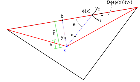
where $\phi_{\delta}(\mathbf{x},\mathbf{a})$ is a dilation of ${\mathbb{R}}^{\ell}$ by the factor $\lVert\phi(\mathbf{x},\mathbf{a})-\mathbf{a}\rVert/\lVert\mathbf{x}-\mathbf{a}\rVert$ and $\phi_{\pi}(\mathbf{x},\mathbf{a})$ is a nonorthogonal projection along $(\mathbf{x}-\mathbf{a})/\lVert\mathbf{x}-\mathbf{a}\rVert$ onto $\tau_{\mathbf{x}}$, the $(\ell-1)$-dimensional face of $\sigma$ containing $\phi(\mathbf{x},\mathbf{a})$. We denote $\hat{r}=\lVert\phi(\mathbf{x},\mathbf{a})-\mathbf{a}\rVert$ and $r=\lVert\mathbf{x}-\mathbf{a}\rVert$. Let $E_{\ell}$ be the $\ell$-hyperplane that contains $\sigma$ and $E_{\ell-1}$ the $(\ell-1)$-hyperplane that contains $\tau_{\mathbf{x}}$. Denote the orthogonal projection of $\mathbf{a}$ onto $E_{\ell-1}$ by $\mathbf{b}$, and let $\hat{h}=\lVert\mathbf{b}-\mathbf{a}\rVert$. For any point $\mathbf{y}=\mathbf{a}+(\mathbf{b}-\mathbf{a})\gamma$ with $0<\gamma<1$, we get $\phi(\mathbf{y},\mathbf{a})=\mathbf{b}$. In particular, we consider the point of intersection of line connecting $\mathbf{a}$ and $\mathbf{b}$ with the $(\ell-1)$-hyperplane parallel to $\tau_{\mathbf{x}}$ that contains $\mathbf{x}$. Naming this point $\mathbf{y}$, we define $h=\lVert\mathbf{y}-\mathbf{a}\rVert$. Let $\mathbf{z}\in E_{\ell}$ denote either normal to $\tau_{\mathbf{x}}$ at $\phi(\mathbf{x},\mathbf{a})$ (either of the two possibilities work). Let $\mathbf{v}_{2}=(\mathbf{x}-\mathbf{a})/\lVert\mathbf{x}-\mathbf{a}\rVert$, and let $\mathbf{v}_{1}$ be the vector in $\operatorname{span}(\mathbf{z},\mathbf{v}_{2})$ that is normal to $\mathbf{v}_{2}$ and points into $\sigma$. We illustrate this construction on a $3$-simplex in Figure 3, where the cone of $\mathbf{a}$ with face $\tau$ is shown in red and the other points and vectors are labeled. We also illustrate the corresponding slice spanned by $\mathbf{v}_{1}$ and $\mathbf{v}_{2}$ in Figure 4.

Figure 3: Illustration of the dilation and nonorthogonal projection involved in retraction for a $3$-simplex.

Figure 4: A $2$-dimensional illustration of the dilation calculation.

Choose an orthogonal basis $\{\mathbf{w}_{1},...,\mathbf{w}_{\ell-2}\}$ for $\operatorname{span}(\mathbf{v}_{1},\mathbf{v}_{2})^{\perp}$. Note that $\operatorname{span}(\mathbf{w}_{1},...,$ $\mathbf{w}_{\ell-2})\subset E_{\ell-1}$. Let $\mathbf{w}^{\prime}$ be a unit vector in $\operatorname{span}(\mathbf{w}_{1},...,\mathbf{w}_{\ell-2})^{\perp}\cap E_{\ell-1}$ parallel to $\,\phi(\mathbf{x})-\mathbf{b}$. Then $\{\mathbf{v}_{1},\mathbf{w}_{1},...,\mathbf{w}_{\ell-2},$ $\mathbf{v}_{2}\}$ is an orthogonal basis for ${\mathbb{R}}^{\ell}$, and $\phi_{\pi}$ is given by

$$\begin{array}[]{rcl}\phi_{\pi}(\mathbf{v}_{1})&=&\alpha\mathbf{w}^{\prime},\\ \phi_{\pi}(\mathbf{w}_{i})&=&\mathbf{w}_{i},\;i\in\{1,...,\ell-2\},~{}~{}\mbox{ and }\\ \phi_{\pi}(\mathbf{v}_{2})&=&0,\end{array}$$ (15)

where $\alpha=\hat{r}/\hat{h}$. Notice that the above set up works everywhere except when $\phi(\mathbf{x})=\mathbf{b}$, in which case we obtain an orthogonal projection for $\phi_{\pi}(\mathbf{x})$ along $\mathbf{b}-\mathbf{a}$. Choosing coordinates for the tangent spaces of $\sigma$ and $\tau_{\mathbf{x}}$ to be $\{\mathbf{v}_{1},\mathbf{w}_{1},...,\mathbf{w}_{\ell-2},\mathbf{v}_{2}\}$ and $\{\mathbf{w}^{\prime},\mathbf{w}_{1},...,$ $\mathbf{w}_{\ell-2}\}$, respectively, we get from Equation (15) that $D\phi_{\pi}(\mathbf{x},\mathbf{a})$ is the $(\ell-1)\times\ell$ matrix given as

$$D\phi_{\pi}(\mathbf{x},\mathbf{a})=\begin{bmatrix}\alpha&0&0&...&0&0\\ 0&1&0&...&0&0\\ \vdots&&\ddots&&\vdots&\vdots\\ 0&\ldots&&&1&0\end{bmatrix}.$$ (16)

5.1.2 Bounding the Integral of the Jacobian

We now present a series of bounds on integrals of the dilation of $d$-volumes induced by the retraction. Since $\ell=d$ implies we are already in the $d$-skeleton and no retraction is needed, we can assume that $\ell>d$. We start with a bound on the maximum dilation of $d$-volumes under the retraction $\phi$. $D\phi$ will denote the tangent map or Jacobian map of $\phi$.

Definition 5.5.

Let $J_{d}\phi(\mathbf{x},\mathbf{a})$ be the maximum dilation of $d$-volumes induced by $D\phi(\mathbf{x},\mathbf{a})$ at $\mathbf{x}$.

We will use the definitions and results on $D\phi_{\pi}(\mathbf{x},\mathbf{a})$ in $\ell$-dimension given above. In particular, recall that $\operatorname{D}(\sigma)$ is the diameter of $\sigma$, $\hat{h}=\|b-a\|$ and $h=\|y-a\|$.

Lemma 5.6.

For any center $\mathbf{a}$ and any point $\mathbf{x}\neq\mathbf{a}$ in the $\ell$-simplex $\sigma$ with $d<\ell\leq p=d+k$,

$$J_{d}\phi(\mathbf{x},\mathbf{a})\leq\left(\frac{\hat{h}}{h}\right)^{d}\frac{\operatorname{D}(\sigma)}{\hat{h}}.$$

Proof.

Following Equation (14), we seek bounds on $D\phi_{\delta}(\mathbf{x},\mathbf{a})$ and $D\phi_{\pi}(\mathbf{x},\mathbf{a})$. Since $D\phi_{\delta}(\mathbf{x},\mathbf{a})$ simply scales by $\hat{r}/r=\hat{h}/h$, the expansion of $d$-volume of any $d$-hyperplane by $D\phi_{\delta}(\mathbf{x},\mathbf{a})$ is by a factor of $(\hat{h}/h)^{d}$. On the other hand, bounding the dilation that $D\phi_{\pi}(\mathbf{x},\mathbf{a})$ can cause in $d$-hyperplanes is a little more involved. We seek a bound on

$$\frac{\sqrt{\det(\,(D\phi_{\pi}(\mathbf{x},\mathbf{a})U)^{T}(D\phi_{\pi}(\mathbf{x},\mathbf{a})U)\,)}}{\sqrt{\det(U^{T}U)}}$$ (17)

for all $\ell\times d$ matrices $U$. Using the generalized Pythagorean theorem [17, Section 1.5], we get

$$\det(U^{T}U)=\sum_{\lambda\in\Lambda}(\det(U_{\lambda}))^{2}$$

where submatrix $U_{\lambda}$ consists of the $d$ rows of $U$ specified by the set of index maps $\Lambda$ given as

$$\lambda\in\Lambda\equiv\{f|f:[1,...,d]\rightarrow[1,...,\ell],~{}f\text{ is one to one and increasing}\}.$$

A similar result holds for $\det((D\phi_{\pi}(\mathbf{x},\mathbf{a})U)^{T}(D\phi_{\pi}(\mathbf{x},\mathbf{a})U))$, with the functions $f$ considered mapping $[1,...,d]$ to $[1,...,\ell-1]$.

Observe that multiplying by $D\phi_{\pi}(\mathbf{x},\mathbf{a})$ (Equation 16) just scales the first row of $U$ by $\alpha$ and removes the last row. Thus $\alpha\det(U_{\lambda})\geq\det((D\phi_{\pi}(\mathbf{x},\mathbf{a})U)_{\lambda})$, which implies that $\alpha$ is a bound on the ratio in Equation (17). Thus we have that

$$J_{d}\phi(\mathbf{x},\mathbf{a})=\left(\frac{\hat{r}}{r}\right)^{d}\frac{\lVert\phi(\mathbf{x},\mathbf{a})-\mathbf{a}\rVert}{\lVert\mathbf{b}-\mathbf{a}\rVert}=\left(\frac{\hat{h}}{h}\right)^{d}\frac{\lVert\phi(\mathbf{x},\mathbf{a})-\mathbf{a}\rVert}{\lVert\mathbf{b}-\mathbf{a}\rVert}\leq\left(\frac{\hat{h}}{h}\right)^{d}\frac{\operatorname{D}(\sigma)}{\hat{h}}$$

holds for all $\mathbf{x}$ and $\mathbf{a}$ in $\sigma$, where $\operatorname{D}(\sigma)$ is the diameter of the $\ell$-simplex $\sigma$. ∎

Next we describe a bound on the integral of $J_{d}\phi(\mathbf{x},\mathbf{a})$ over the entire $\ell$-simplex, for a fixed center $\mathbf{a}$. We will find that this bound is independent of the position of $\mathbf{a}$. Recall that $\operatorname{Per}(\sigma)$ and $\operatorname{P}(\sigma)$ denote the perimeter of $\ell$-simplex $\sigma$ and the $(\ell-1)$-dimensional volume of the perimeter, respectively, and $\operatorname{Int}(\sigma)$ its interior.

Lemma 5.7.

For any fixed center $\mathbf{a}$ in the $\ell$-simplex $\sigma$ with $d<\ell\leq p=d+k$,

$$\int_{\operatorname{Int}(\sigma)}J_{d}\phi(\mathbf{x},\mathbf{a})\,{\rm d}{\mathcal{L}}^{\ell}(\mathbf{x})\,\leq\,\operatorname{D}(\sigma)\operatorname{P}(\sigma).$$

Proof.

Consider the $(\ell-1)$-dimensional faces $\tau_{j}$ of $\sigma$, with $\operatorname{Per}(\sigma)=\{\cup_{j}\tau_{j}\,|\,\tau_{j}\in\sigma,\,\dim(\tau_{j})=\ell-1\}$. Let $\sigma_{j}$ denote the $\ell$-simplex generated by $\mathbf{a}$ and $\tau_{j}$. Then

$$\int_{\operatorname{Int}(\sigma)}J_{d}\phi(\mathbf{x},\mathbf{a})\,{\rm d}{\mathcal{L}}^{\ell}(\mathbf{x})=\sum_{j}\int_{\operatorname{Int}(\sigma_{j})}J_{d}\phi(\mathbf{x},\mathbf{a})\,{\rm d}{\mathcal{L}}^{\ell}(\mathbf{x}).$$

Let $\tau_{j}(h)$ denote the $(\ell-1)$-simplex formed by the intersection of $\sigma_{j}$ and the $(\ell-1)$-hyperplane parallel to $\tau_{j}$ at a distance $h$ from $\mathbf{a}$. Thus, $\tau_{j}(\hat{h})$ is $\tau$ itself. We observe that our bound on $J_{d}\phi(\mathbf{x},\mathbf{a})$ is constant in $\tau_{j}(h)$ for any $h$. The $(\ell-1)$-dimensional volume of $\tau_{j}(h)$ is given by

$$\operatorname{V}_{\ell-1}(\tau_{j}(h))=\left(\frac{h}{\hat{h}}\right)^{\ell-1}\operatorname{V}_{\ell-1}(\tau_{j}).$$

Using the bound on $J_{d}\phi(\mathbf{x},\mathbf{a})$ from Lemma 5.6, and noting that $\operatorname{D}(\sigma_{j})\leq\operatorname{D}(\sigma)~{}\forall\,j$, we get

$$\int_{\operatorname{Int}(\sigma_{j})}J_{d}\phi(\mathbf{x},\mathbf{a})\,{\rm d}{\mathcal{L}}^{\ell}(\mathbf{x})\leq\int_{0}^{\hat{h}}\left(\frac{h}{\hat{h}}\right)^{\ell-1}\operatorname{V}_{\ell-1}(\tau_{j})\,\left(\frac{\hat{h}}{h}\right)^{d}\frac{\operatorname{D}(\sigma)}{\hat{h}}\,{\rm d}h=\frac{\operatorname{V}_{\ell-1}(\tau_{j})\operatorname{D}(\sigma)}{\ell-d}.$$

Summing this quantity over all $\tau_{j}\in\operatorname{Per}(\sigma)$ and replacing $\ell-d\geq 1$ with $1$ gives the overall bound. ∎

We now bound the integral of $J_{d}\phi(\mathbf{x},\mathbf{a})$ over centers $\mathbf{a}$ with a fixed $\mathbf{x}$ that we are retracting onto $\operatorname{Per}(\sigma)$. Examination of the corresponding proof for the original deformation theorem [17, Section 7.7] shows that symmetry of the cubical mesh plays a very special role, which cannot be duplicated in the case of simplicial complex. In particular, we must avoid integrating over $\mathbf{a}$ close to the perimeter of $\sigma$. Hence we integrate over as big a region as we can while still avoiding a neighborhood of the perimeter. As in the statement of the main Theorem 5.1, let $\hat{\cal B}_{\sigma}$ be the largest ball inscribed in $\sigma$, ${\cal B}_{\sigma}$ be the ball with half the radius and same center as $\hat{\cal B}_{\sigma}$, and $r_{\sigma}$ be the radius of ${\cal B}_{\sigma}$.

Lemma 5.8.

For any point $\mathbf{x}$ in the $\ell$-simplex $\sigma$ with $d<\ell\leq p=d+k$,

$$\int_{{\cal B}_{\sigma}}J_{d}\phi(\mathbf{x},\mathbf{a})\,{\rm d}{\cal L}^{\ell}(\mathbf{a})\,\leq\,\operatorname{D}(\sigma)\operatorname{P}(\sigma)+\operatorname{V}_{\ell}({\cal B}_{\sigma})\frac{\operatorname{D}(\sigma)}{r_{\sigma}}.$$

Proof.

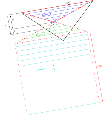
Similar to the subsimplices of $\sigma$ considered in the Proof of Lemma 5.7, let $\sigma_{j}$ now denote the $\ell$-simplex formed by $\mathbf{x}$ and $\tau_{j}\in\operatorname{Per}(\sigma)$. In order to derive an upper bound, we integrate instead over regions that are by construction bigger than these subsimplices of $\sigma$. Denoting the simplex $\sigma_{j}$ as Region 1, we define Regions 2 and 3 as follows. We refer the reader to Figure 5 for an illustration of this construction. Let $\sigma^{\prime}_{j}$ be the reflection of $\sigma_{j}$ through $\mathbf{x}$, and similarly, let $\tau^{\prime}_{j}$ be the reflection through $\mathbf{x}$ of $\tau_{j}$. We define $\sigma^{\prime}_{j}$ as Region 2. Notice that unlike Region 1, Region 2 need not be contained fully in $\sigma$. As defined in Section 5.1.1, let $\mathbf{z}$ be the unit vector normal to the $(\ell-1)$-hyperplane containing $\tau_{j}$ pointing into $\sigma$. We define Region 3 as the $\ell$-dimensional set $\,\tau^{\prime}_{j}+[0,\operatorname{D}(\sigma)]\mathbf{z}$, as illustrated in Figure 5.

Note that the union of all Region 2’s and Region 3’s cover $\sigma$. By an argument almost identical to that above, we have the following upper bound on the integrand in question.

$$\left(\frac{h^{\prime}}{h}\right)^{d}\frac{\lVert\phi(\mathbf{x},\mathbf{a})-\mathbf{a}\rVert}{\hat{h}}\,\leq\,\left(\frac{h^{\prime}}{h}\right)^{d}\frac{\operatorname{D}(\sigma)}{\hat{h}}.$$

Figure 5: Illustration for integration of Jacobian bound over centers $\mathbf{a}$ instead of $\mathbf{x}$’s. For the case of the triangle shown, there will be 3 sets of 3 regions. In general there will be 3 regions for every face of the simplex.

Integrating the second of these two terms over Region 2 and summing the integral over all such Regions 2 for all faces $\tau_{j}$, we get the upper bound of $\operatorname{D}(\sigma)\operatorname{P}(\sigma)$. Here we use the same arguments as the ones employed in Lemma 5.7. Region 2 alone is not guaranteed to cover ${\cal B}_{\sigma}$ as some of ${\cal B_{\sigma}}$ may occupy parts of Region 3. Since $\mathbf{a}\in{\cal B}_{\sigma}$, we have $\hat{h}>r_{\sigma}$, and $h^{\prime}\leq h$ when $\mathbf{a}\in$Region 3, so that

$$\left(\frac{h^{\prime}}{h}\right)^{d}\frac{\operatorname{D}(\sigma)}{\hat{h}}\leq\frac{\operatorname{D}(\sigma)}{r_{\sigma}}.$$

Combining the above estimates while integrating over all such Regions 2 and 3 gives us the bound specified in the Lemma. ∎

5.1.3 Bounding the pushforwards of the current

We consider the $d$-current $T$, and employ the bounds on the Jacobian of retraction described above to the pushforwards of $T$ and its boundary $\partial T$ on to the simplicial complex $K$. Our treatment of the pushforwards essentially follows the corresponding results of Krantz and Parks for the case of square grid [17, Pages 218–219]. We denote by $\lVert T\rVert$ the total variation measure of the current $T$, which is determined by the identity

$$\lVert T\rVert(W)=\sup_{\text{\parbox{63.00014pt}{\centering$\omega\in\mathcal{D}^{d}$, $\lVert\omega\rVert=1$,\\ $\operatorname{spt}\omega\subset W$\@add@centering}}}T(\omega).$$

Lemma 5.9.

Suppose $K$ is a $p$-dimensional simplicial complex with $p=d+k$ for $k\geq 1$. Consider the stepwise retraction of the $d$-current $T\subset K$ (the $(d-1)$-current $\partial T\subset K$) onto the $d$-skeleton of $K$ (respectively, the $(d-1)$-skeleton of $K$). Each step of the retraction on to the perimeter of an $\ell$-simplex $\sigma$ for $d<\ell\leq p$ (respectively, $d\leq\ell\leq p$) increases the mass of $T$ or $\partial T$ by at most a factor of

$$4\upvartheta_{K}=4(\upkappa_{1}+\upkappa_{2})=4\max_{\sigma\in K}\left(\frac{\operatorname{D}(\sigma)\operatorname{P}(\sigma)}{\operatorname{V}_{\ell}({\cal B}_{\sigma})}+\frac{\operatorname{D}(\sigma)}{r_{\sigma}}\right).$$

Proof.

Using Fubini’s theorem [17, Page 26] and applying the bound in Lemma 5.8, we get

$$\int_{{\cal B}_{\sigma}}\int_{\sigma}J_{d}\phi(\mathbf{x},\mathbf{a})\,{\rm d}\lVert T\rVert(\mathbf{x})\,{\rm d}{\cal L}^{\ell}(\mathbf{a})=\int_{\sigma}\int_{{\cal B}_{\sigma}}J_{d}\phi(\mathbf{x},\mathbf{a})\,{\rm d}{\cal L}^{\ell}(\mathbf{a})\,{\rm d}\lVert T\rVert(\mathbf{x})\,\leq\,\upvartheta_{\sigma}\operatorname{M}(T|_{\sigma}),$$

where $\upvartheta_{\sigma}=\operatorname{D}(\sigma)\operatorname{P}(\sigma)+\operatorname{V}_{d}({\cal B}_{\sigma})(\operatorname{D}(\sigma)/r_{\sigma})\,$ and $T|_{\sigma}\,$ is the portion of the current $T$ restricted to the simplex $\sigma$. Consider the subset of ${\cal B}_{\sigma}$ defined as

$$H_{T}=\left\{\mathbf{a}\in{\cal B}_{\sigma}\,\big{|}\,\int_{\sigma}J_{d}\phi(\mathbf{x},\mathbf{a})\,{\rm d}\lVert T\rVert(\mathbf{x})>\frac{4\upvartheta_{\sigma}\operatorname{M}(T|_{\sigma})}{\operatorname{V}_{\ell}({\cal B}_{\sigma})}\right\}.$$

Then $\operatorname{V}_{\ell}(H_{T})\leq(1/3)\operatorname{V}_{\ell}({\cal B}_{\sigma})$. Similarly we define $H_{\partial T}$ for the pushforward of $\partial T$ and get $\operatorname{V}_{\ell}(H_{\partial T})\leq(1/3)\operatorname{V}_{\ell}({\cal B}_{\sigma})$. Then the set $\,{\cal B}_{\sigma}\setminus\{H_{T}\cup H_{\partial T}\}\,$ defines a subset of ${\cal B}_{\sigma}$ with positive measure, with the centers $\mathbf{a}$ in this subset satisfying $\,\int_{\sigma}J_{d}\phi(\mathbf{x},\mathbf{a})\,{\rm d}\lVert T\rVert(\mathbf{x})\,\leq\,4\upvartheta_{\sigma}\operatorname{M}(T|_{\sigma})/\operatorname{V}_{\ell}({\cal B}_{\sigma})\,$ and $\,\int_{\sigma}J_{d}\phi(\mathbf{x},\mathbf{a})\,{\rm d}\lVert\partial T\rVert(\mathbf{x})\,\leq\,4\upvartheta_{\sigma}\operatorname{M}(T|_{\sigma})/\operatorname{V}_{\ell}({\cal B}_{\sigma})$. Hence we can choose centers to retract from in each simplex $\sigma$ such that the expansion of mass of the current restricted to that simplex is bounded by $4\upvartheta_{\sigma}/\operatorname{V}_{\ell}({\cal B}_{\sigma})$. The bound specified in the Lemma follows when we consider retracting the entire current over multiple simplices in $K$, and set $\upvartheta_{K}=\max_{\sigma\in K}\upvartheta_{\sigma}$ as the generic upper bound that holds for all simplices in $K$. ∎

Bound on complete sequence of retractions.

We can apply the bound specified in Lemma 5.9 over multiple levels $\ell$. Pushing $T$ onto the $d$-skeleton of $p$-complex $K$ multiplies the mass of $T$ by a factor of at most $(4\upvartheta_{K})^{k}$. Likewise, pushing $\partial T$ on to the $(d-1)$-skeleton multiplies the mass of $\partial T$ by a factor of at most $(4\upvartheta_{K})^{k+1}$.

5.1.4 Bounding the distance between the current and its simplicial approximation

In the final step, we construct the simplicial current $P$ approximating the original current $T$, and bound the flat norm distance between the two. Since we are now considering retraction maps over many simplices simultaneously, we let $\phi_{i}$ denote the global projection from the $(p-i+1)-$skeleton to the $(p-i)-$skeleton, suppressing the particular $\mathbf{x}$ and $\mathbf{a}$. We denote the composition of all these steps as $\psi^{1}\equiv\phi_{k}\circ\dots\circ\phi_{1}$ and hence we map $T$ forward by $\psi^{1}$, picking centers (see Lemma 5.8) to project from in each step and in each simplex. We pick each of these centers such that the retractions map $\partial T$ with bounded amplification of mass as well (see Lemma 5.9).

The homotopy formula [17, Section 7.4.3] states that given a smooth homotopy $g$ from $f_{0}$ to $f_{1}$ where $f_{0},f_{1}:U\subseteq{\mathbb{R}}^{n_{0}}\to{\mathbb{R}}^{n_{1}}$ are smooth functions with $g(0,x)=f_{0}(x)$ and $g(1,x)=f_{1}(x)$, if $T$ is a $d$-current and $f^{-1}(F)\cap\operatorname{spt}f$ is compact for every compact set $F\subseteq{\mathbb{R}}^{n_{1}}$, we have that the difference in pushforwards of $T$ under $f_{1}$ and $f_{0}$ is given by

$${f_{1}}_{\#}(T)-{f_{0}}_{\#}(T)=\partial g_{\#}([0,1]\times T)+g_{\#}([0,1]\times\partial T).$$

Define the homotopy $g(\gamma,\mathbf{x})=\gamma\mathbf{x}+(1-\gamma)\psi^{1}(\mathbf{x})$ for $\gamma\in[0,1]$. Then the homotopy formula gives

$$T-\psi^{1}_{\#}(T)=\partial g_{\#}([0,1]\times T)+g_{\#}([0,1]\times\partial T).$$

We define $R=g_{\#}([0,1]\times T)$ and $Q_{1}=g_{\#}([0,1]\times\partial T)$. Then we get

$$T-\psi^{1}_{\#}(T)=\partial R+Q_{1}.$$ (18)

Finally, we map $\psi^{1}_{\#}(\partial T)$ forward to the $(d-1)$-skeleton of simplicial complex $K$ with $\phi=\phi_{k+1}$ to get $\psi^{2}_{\#}(\partial T)=\phi_{\#}(\psi^{1}_{\#}(\partial T))$. For this purpose, consider the homotopy $h(\gamma,\mathbf{x})$ from $\psi^{1}_{\#}(\partial T)$ to $\psi^{2}_{\#}(\partial T)$, i.e.,

$$h(\gamma,x)=\gamma\psi^{1}_{\#}(\mathbf{x})+(1-\gamma)\psi^{2}_{\#}(\mathbf{x})~{}\mbox{ for }~{}\gamma\in[0,1].$$

We define

$$P=\psi^{1}_{\#}(T)-h_{\#}([0,1]\times\psi^{1}_{\#}(\partial T)).$$ (19)

$P$ is a $d$-current whose boundary $\partial P$ is contained in the $(d-1)$-skeleton of $K$. Define $Q_{2}=h_{\#}([0,1]\times\psi^{1}_{\#}(\partial T))$. Using the homotopy formula, we get

$$\partial P =\partial\left(\,\psi^{1}_{\#}(T)-h_{\#}([0,1]\times\psi^{1}_{\#}(\partial T))\,\right)$$

$$=\,\psi^{1}_{\#}(\partial T)-\partial h_{\#}([0,1]\times\psi^{1}_{\#}(\partial T))\,$$

$$=\psi^{2}_{\#}(\partial T)\subset(d-1)\text{-skeleton of }K.$$

Equation (19) gives $\psi^{1}_{\#}(T)=P+Q2$. Defining $Q=Q_{1}+Q_{2}$, Equation (18) gives

$$T-(P+Q2) =\partial R+Q_{1},~{}~{}\mbox{hence }$$

$$T-P =\partial R+Q.$$

Finally, we apply the bounds on the retraction described in Lemma 5.9 and the paragraph following this Lemma to the masses of the pushforwards. Noticing that $\operatorname{D}(\sigma)\leq\Updelta$ for all $\sigma\in K$, we get the following bounds, which finish the proof of our simplicial deformation theorem (Theorem 5.1).

$$\operatorname{M}(P) \leq(4\upvartheta_{K})^{k}\operatorname{M}(T)+\Updelta(4\upvartheta_{K})^{k+1}\operatorname{M}(\partial T)$$

$$=(4\upvartheta_{K})^{k}\left(\operatorname{M}(T)+\Updelta(4\upvartheta_{K})\operatorname{M}(\partial T)\right),$$

$$\operatorname{M}(\partial P) \leq(4\upvartheta_{K})^{k+1}\operatorname{M}(\partial T),$$

$$\operatorname{M}(R) \leq\Updelta\operatorname{M}(\psi^{1}_{\#}(T))$$

$$\leq\Updelta(4\upvartheta_{K})^{k}\operatorname{M}(T),~{}\mbox{ and }$$

$$\operatorname{M}(Q) \leq\Updelta(4\upvartheta_{K})^{k}\operatorname{M}(\partial T)+\Updelta(4\upvartheta_{K})^{k+1}\operatorname{M}(\partial T)$$

$$=\Updelta(4\upvartheta_{K})^{k}(1+4\upvartheta_{K})\operatorname{M}(\partial T).$$

∎

Remark 5.10.

The influence of Simplicial regularity as measured by $\upkappa_{1}$ and $\upkappa_{2}$ is clearly revealed by the statement of our deformation theorem (Theorem 5.1). Explicit constants are a simple yet useful part of the result; as observed above in Remark 5.2, the statement of this theorem leads to an easy observation that the flat norm distance between $T$ and $P$ can be made a small as desired by subdividing the simplicial complex in a manner that keeps the regularity constants bounded. This can be done, for example, by using the subdivision algorithm of Edelsbrunner and Grayson [12].

Remark 5.11.

We did not explicitly discuss the case of $0$-dimensional currents. In this case, the bounds on mass expansion are all equal to one.

5.2 Comparison of Bounds of Approximation

Sullivan studied the deformation of integral currents on to the skeleton of a cell complex, which is composed of compact convex sets. He presented a deformation theorem for deforming integral currents on to the boundary of a cell complex [26, Theorem 4.5]. For ease of comparison, we use our notation to restate the bounds given by Sullivan for deforming a $d$-current $T$ to a polyhedral current $P$ in the boundary of a cell complex in ${\mathbb{R}}^{q}$. Recall that in our simplicial deformation theorem (Theorem 5.1), the simplicial complex considered has dimension $p$ and is embedded in ${\mathbb{R}}^{q}$ for $q\geq p$. Furthermore, $\upkappa_{1}$, $\upkappa_{2}$, $\Updelta$, and $\upvartheta_{K}$ are simplicial regularity constants. We also note that even though Sullivan stated his results for full-dimensional complexes and the standard flat norm, it is straightforward to extend them to lower dimensional complexes and the flat norm with scale:

$$\operatorname{M}(P) ~{}\leq~{}{p\choose d}\left(2d\left(\frac{d+1}{2d}\upkappa_{2}\right)^{d+1}\right)^{p-d+1}\operatorname{M}(T),$$ (20)

$$\operatorname{M}(\partial P) ~{}\leq~{}{p\choose d-1}\left(2d\left(\frac{d+1}{2d}\upkappa_{2}\right)^{d}\right)^{p-d+1}\operatorname{M}(\partial T),~{}~{}~{}\mbox{and}$$ (21)

$${\mathbb{F}}_{\lambda}(T,P) ~{}=~{}\lambda^{d}\cdot{\mathbb{F}}_{1}(T/\lambda,P/\lambda)$$

$$~{}\leq~{}\lambda^{d}\cdot(p-d+1)\Updelta\,(\,\operatorname{M}(P/\lambda)+\operatorname{M}(\partial P/\lambda)\,)$$

$$~{}=\lambda^{d}\cdot(p-d+1)\Updelta\,(\,\lambda^{-d}\cdot\operatorname{M}(P)+\lambda^{1-d}\cdot\operatorname{M}(\partial P)\,)$$

$$~{}=(p-d+1)\Updelta\,(\,\operatorname{M}(P)+\lambda\operatorname{M}(\partial P)\,).$$ (22)

Our results corresponding to the first two bounds in Equations (20) and (21) are presented in Equations (10) and (11) in Theorem 5.1, which we repeat here with the substitution $k=p-d$.

$$\operatorname{M}(P) \leq(4\upvartheta_{K})^{p-d}\operatorname{M}(T)+\Updelta(4\upvartheta_{K})^{p-d+1}\operatorname{M}(\partial T),$$ (10 revisited)

$$\operatorname{M}(\partial P) \leq(4\upvartheta_{K})^{p-d+1}\operatorname{M}(\partial T),$$ (11 revisited)

$$\operatorname{M}(R) \leq\Updelta(4\upvartheta_{K})^{p-d}\operatorname{M}(T),\mbox{ and}$$ (12 revisited)

$$\operatorname{M}(Q) \leq\Updelta(4\upvartheta_{K})^{p-d}(1+4\upvartheta_{K})\operatorname{M}(\partial T).$$ (13 revisited)

To obtain the flat norm distance corresponding to the third bound given by Sullivan in Equation (22), we use the definition of flat norm distance between two currents specified in Equation (2). Using $T-P=\partial Q+R$, we combine two of our bounds specified in Equations (12) and (13) to get

$${\mathbb{F}}_{\lambda}(T,P) ~{}\leq~{}\Updelta(4\upvartheta_{K})^{p-d}\,\left(\,\operatorname{M}(T)+\lambda(1+4\upvartheta_{K})\operatorname{M}(\partial T)\,\right).\hskip 36.135pt$$

To gain a better understanding of how the two sets of bounds compare, we compute these bounds explicitly for the case of a $2$-current in a regular tetrahedral complex (thus, $p=3$ and $d=2$). Notice that this instance is close to a best case for Sullivan’s bounds, as less regular complexes affect them more severely. With this point in mind, we present in Table 1 our bounds and Sullivan’s bounds on both a regular tetrahedral complex and one on which we stretch the regular tetrahedra by a factor of 10 in a direction normal to one of their faces (i.e., turn them into skinny, spike-like simplices).

Quantity	Sullivan’s bound	Our bound
Regular tetrahedra
$M(P)$	$(1.2\times 10^{5})\,\operatorname{M}(T)$	$$(1.6\times 10^{3})\,\operatorname{M}(T)\\ +(2.5\times 10^{6})\,\Updelta\operatorname{M}(\partial T)$$
$M(\partial P)$	$(8.7\times 10^{3})\,\operatorname{M}(\partial T)$	$(2.5\times 10^{6})\,\operatorname{M}(\partial T)$
${\mathbb{F}}_{\lambda}(T,P)$	$$(2.4\times 10^{5})\,\Updelta\operatorname{M}(T)\\ +(1.7\times 10^{3})\,\Updelta\lambda\operatorname{M}(\partial T)$$	$$(1.6\times 10^{3})\,\Updelta\operatorname{M}(T)\\ +(2.5\times 10^{6})\,\Updelta\lambda\operatorname{M}(\partial T)$$
Stretched tetrahedra
$M(P)$	$(5.5\times 10^{9})\,\operatorname{M}(T)$	$$(3.7\times 10^{4})\,\operatorname{M}(T)\\ +(1.4\times 10^{9})\,\Updelta\operatorname{M}(\partial T)$$
$M(\partial P)$	$(1.1\times 10^{7})\,\operatorname{M}(\partial T)$	$(1.4\times 10^{9})\,\operatorname{M}(\partial T)$
${\mathbb{F}}_{\lambda}(T,P)$	$$(1.1\times 10^{10})\Updelta\operatorname{M}(T)\\ +(2.3\times 10^{7})\Updelta\lambda\operatorname{M}(\partial T)$$	$$(3.7\times 10^{4})\,\Updelta\operatorname{M}(T)\\ +(1.4\times 10^{9})\Updelta\lambda\operatorname{M}(\partial T)$$

Table 1: Comparison of our bounds with those obtained by Sullivan for a 2-current in a (1) 3-complex of congruent regular tetrahedra and (2) a 3-complex of congruent stretched tetrahedra which are created by taking regular tetrahedra and multiplying their height by a factor of 10.

For the regular tetrahedral complex and the $\operatorname{M}(P)$ bound, our coefficient of $\operatorname{M}(T)$ is more than $74$ times better, but we do have a second term that can be quite large, but diminishes in importance if the complex is subdivided appropriately (see Remark 5.10). In the stretched complex, our coefficient on $\operatorname{M}(T)$ is $1.5\times 10^{5}$ times better, indicating that our bound is better behaved for irregular complexes. Our bound on $\operatorname{M}(\partial P)$ is about $290$ times worse than Sullivan’s for the regular tetrahedra, and about $120$ times worse for the stretched complex. For the flat norm bound in the regular complex, we are about $148$ times better on the $\operatorname{M}(T)$ term and about $145$ times worse on the $\operatorname{M}(\partial T)$ term. On the stretched complex, our $\operatorname{M}(T)$ coefficient is about $3\times 10^{5}$ times better, and our $\operatorname{M}(\partial T)$ coefficient is about $60$ times worse. We also note that in the case of the flat norm with scale, our larger $\operatorname{M}(\partial T)$ coefficient becomes less important for small $\lambda$.

Remark 5.12.

For the important case where $\partial T$ is empty, i.e., when $T$ is a cycle, we have $\operatorname{M}(\partial T)=0$, and hence our bounds are uniformly better than Sullivan’s.

As compared to Sullivan, we are able to take advantage of our simplicial setting to get better bounds on the mass expansion of $T$. While our mass expansion bounds involving $\partial T$ are currently inferior to Sullivan’s, we suspect our arguments can be tightened and modified to obtain bounds that are better in all cases. More importantly, our bounds are less sensitive to simplicial irregularity. Given the challenges inherent in creating meshes without slivers even in three dimensions [5], bounds that behave well in their presence are highly desirable.

6 Computational Results

We illustrate computations of the multiscale simplicial flat norm by describing the flat norm decompositions of a $2$-manifold with boundary embedded in ${\mathbb{R}}^{3}$ (see Figure 6). The input set has the underlying shape of a pyramid, to which several peaks and troughs of varying scale, as well as random noise, have been added. We model this set as a piecewise linear $2$-manifold with boundary, and find a triangulation of the same as a subcomplex of a tetrahedralization of the $2\times 2\times 2$ cube centered at the origin, within which the set is located. We use the method of constrained Delaunay tetrahedralization [25] implemented in the package TetGen [23] for this purpose. We then compute the multiscale simplicial flat norm decomposition of the input set at various scale ($\lambda$) values. At high values, e.g., when $\lambda=6$, the optimal decomposition resembles the input set with the small kinks due to random noise smoothed out. At the other end, for $\lambda=0.01$, the optimal decomposition resembles a flat “sheet”. For intermediate values of $\lambda$, the optimal decomposition captures features of the input set at varying scales.

Figure 6: Top left: A view of original pyramidal surface in three dimensions. The remaining three figures show the flat norm decomposition for scales $\lambda=6$ (top right), $\lambda=2$ (bottom left), and $\lambda=0.01$ (bottom right). See text for further explanation. The images were generated using the package TetView [24].

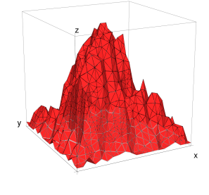
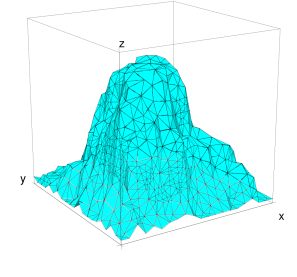
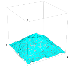
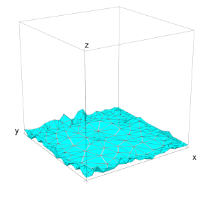
The entire $3$-complex mesh modeling the cube in question consisted of 14,002 tetrahedra and 28,844 triangles. For each $\lambda$, computation of the multiscale simplicial flat norm described above took only a few minutes on a regular PC using standard functions from MATLAB. This example demonstrates the feasibility of efficiently computing flat norm decompositions of large datasets in high dimensions, for the purposes of denoising or to recover scale information of the data.

7 Discussion

Our result on simplicial deformation (Theorem 5.1) places the definition of the multiscale simplicial flat norm into clear context. If a current lives in the underlying space of a simplicial complex, we can deform it to be a simplicial current on the simplicial complex, and do so with controlled error. In fact, by subdividing the simplicial complex carefully, we can move this error as close to zero as we like. Since the multiscale simplicial flat norm could be computed efficiently when the simplicial complex does not have relative torsion, one could naturally use our approach to compute the flat norm of a large majority of currents in arbitrarily large dimensions. An important open question in this context is whether the multiscale simplicial flat norm of a current on a simplicial complex with relative torsion could be approximated efficiently by coarsening the complex so that the relative torsion is removed. For instance, it has been observed recently that edge contractions could remove existing relative torsion while preserving the homology groups of the simplicial complex in certain cases [9].

The multiscale simplicial flat norm problem, similar to the recent results on the optimal bounding chain problem [10], apply notions from algebraic topology and discrete optimization to problems from geometric measure theory such as flat norm of currents and area-minimizing hypersurfaces. What other classes of problems from the broader area of geometric analysis could we tackle using similar approaches? One such question appears to be the following: under what conditions is the flat norm decomposition of an integral current guaranteed to be another integral current? Working in the setting of simplicial complexes, results on the existence of integral optimal solutions for instances of ILPs with integer right-hand side vectors may prove useful in answering this question.

While $L^{1}$TV and flat norm computations have been used widely on data in two dimensions, such as images, the multiscale simplicial flat norm opens up the possibility of utilizing flat norm computations for higher dimensional data. Similar to the flat norm-based signatures for distinguishing shapes in two dimensions [29], could we define shape signatures using multiscale simplicial flat norm computations to characterize the geometry of sets in arbitrary dimensions? The sequence of optimal multiscale simplicial flat norm decompositions of a given set for varying values of the scale parameter $\lambda$ captures all the scale information of its geometry. Could we represent all this information in a compact manner, for instance, in the form of a barcode?

References

- [1] Ian Agol, Joel Hass, and William Thurston. The computational complexity of knot genus and spanning area. Transactions of the American Mathematical Society, 358(9):3821–3850, 2006.
- [2] Dimitris Bertsimas and John N. Tsitsiklis. Introduction to Linear Optimization. Athena Scientific, Belmont, MA., 1997.
- [3] Tony F. Chan and Selim Esedoglu. Aspects of total variation regularized function approximation. SIAM Journal on Applied Mathematics, 65(5):1817–1837, 2005.
- [4] Chao Chen and Daniel Freedman. Hardness results for homology localization. In SODA ’10: Proc. 21st Ann. ACM-SIAM Sympos. Discrete Algorithms, pages 1594–1604, 2010.
- [5] Siu-Wing Cheng, Tamal Dey, and Jonathan Shewchuk. Delaunay Mesh Generation. CRC Press, 2012.
- [6] Vin de Silva and Robert Ghrist. Coordinate-free coverage in sensor networks with controlled boundaries via homology. International Journal of Robotics Research, 25(12):1205–1222, 2006.
- [7] Vin de Silva and Robert Ghrist. Coverage in sensor networks via persistent homology. Algebraic and Geometric Topology, 7:339–358, 2007.
- [8] Tamal K. Dey, Anil N. Hirani, and Bala Krishnamoorthy. Optimal homologous cycles, total unimodularity, and linear programming. In STOC ’10: Proc. 42nd Ann. Sympos. Theo. Comput., pages 221–230, 2010.
- [9] Tamal K. Dey, Anil N. Hirani, Bala Krishnamoorthy, and Gavin W. Smith. Edge contractions and simplicial homology. 2013. arxiv:1304.0664.
- [10] Nathan M. Dunfield and Anil N. Hirani. The least spanning area of a knot and the optimal bounding chain problem. In Prooceedings of the 27th ACM Annual Symposium on Computational Geometry, SoCG ’11, pages 135–144, 2011.
- [11] Herbert Edelsbrunner. Geometry and Topology for Mesh Generation. Cambridge Monographs on Applied and Computational Mathematics. Cambridge University Press, New York, NY, USA, 2006.
- [12] Herbert Edelsbrunner and Daniel Grayson. Edgewise subdivision of a simplex. Discrete Computational Geometry, 24:707–719, 2000.
- [13] Herbert Federer. Geometric Measure Theory. Die Grundlehren der mathematischen Wissenschaften, Band 153. Springer-Verlag, New York, 1969.
- [14] Donald Goldfarb and Wotao Yin. Parametric maximum flow algorithms for fast total variation minimization. SIAM Journal on Scientific Computing, 31(5):3712–3743, 2009.
- [15] Osman Güler, Dick den Hertog, Cornelis Roos, Tamas Terlaky, and Takashi Tsuchiya. Degeneracy in interior point methods for linear programming: a survey. Annals of Operations Research, 46-47(1):107–138, March 1993.
- [16] Vladimir Kolmogorov and Ramin Zabih. What energy functions can be minimized via graph cuts? In Proceedings of the 7th European Conference on Computer Vision-Part III, ECCV ’02, pages 65–81, London, UK, UK, 2002. Springer-Verlag.
- [17] Steven G. Krantz and Harold R. Parks. Geometric Integration Theory. Cornerstones. Birkhauser, 2008.
- [18] Frank Morgan. Geometric Measure Theory: A Beginner’s Guide. Academic Press, fourth edition, 2008.
- [19] Simon P. Morgan and Kevin R. Vixie. TV computes the flat norm for boundaries. Abstract and Applied Analysis, 2007:Article ID 45153,14 pages, 2007.
- [20] James R. Munkres. Elements of Algebraic Topology. Addison–Wesley Publishing Company, Menlo Park, 1984.
- [21] Henri Poincaré. Papers on Topology: Analysis Situs and Its Five Supplements. History of Mathematics. American Mathematical Society, 2010.
- [22] Alexander Schrijver. Theory of Linear and Integer Programming. Wiley-Interscience Series in Discrete Mathematics. John Wiley & Sons Ltd., Chichester, 1986.
- [23] Hang Si. TetGen: A quality tetrahedral mesh generator and a 3D Delaunay triangulator. Available at http://tetgen.berlios.de.
- [24] Hang Si. TetView: A tetrahedral mesh and piecewise linear complex viewer. Available at http://tetgen.berlios.de/tetview.html.
- [25] Hang Si. Constrained Delaunay tetrahedral mesh generation and refinement. Finite Elements in Analysis and Design, 46:33–46, January 2010.
- [26] John M. Sullivan. A Crystalline Approximation Theorem for Hypersurfaces. PhD thesis, Princeton University, 1990.
- [27] Éva Tardos. A strongly polynomial algorithm to solve combinatorial linear programs. Operations Research, 34(2):250–256, March 1986.
- [28] Arthur F. Veinott, Jr. and George B. Dantzig. Integral extreme points. SIAM Review, 10(3):371–372, 1968.
- [29] Kevin R. Vixie, Keith Clawson, Thomas J. Asaki, Gary Sandine, Simon P. Morgan, and Brandon Price. Multiscale flat norm signatures for shapes and images. Applied Mathematical Sciences, 4(13-16):667–680, 2010.