Anisotropic Cosmological Model in Modified Brans–Dicke Theory

Abstract

Recently, it has been shown that a four–dimensional ($4D$) Brans–Dicke (BD) theory with an effective matter field and a self interacting potential can be achieved from the vacuum $5D$ BD field equations, where we refer to as a modified Brans–Dicke theory (MBDT). We investigate a generalized Bianchi type I anisotropic cosmology in $5D$ BD theory, and by employing the obtained formalism, we derive the induced–matter on any $4D$ hypersurface in the context of the MBDT. We illustrate that if the usual spatial scale factors are functions of the time while the scale factor of extra dimension is constant, and the scalar field depends on the time and the fifth coordinate, then in general, one will encounter inconsistencies in the field equations. Then, we assume the scale factors and the scalar field depend on the time and the extra coordinate as separated variables in the power–law forms. Hence, we find a few classes of solutions in $5D$ space–time through which, we probe the one which leads to a generalized Kasner relations among the Kasner parameters. The induced scalar potential is found to be in the power–law or in the logarithmic form, however, for a constant scaler field and even when the scalar field only depends on the fifth coordinate, it vanishes. The conservation law is indeed valid in this MBDT approach for the derived induced energy–momentum tensor (EMT). We proceed our investigations for a few cosmological quantities, where for simplicity we assume the metric and the scalar field are functions of the time. Hence, the EMT satisfies the barotropic equation of state, and the model indicates that constant mean Hubble parameter is not allowed. Thus, by appealing to the variation of Hubble parameter, we assume a fixed deceleration parameter, and set the evolution of the quantities with respect to the fixed deceleration, the BD coupling and the state parameters. The WEC allows a shrinking extra dimension for a decelerating expanding universe that, in the constant scalar field, evolves the same as the flat FRW space–time in GR. The quantities for the stiff fluid and the radiation dominated universe indicate an expanding universe commenced with a big bang. There is a horizon for each of the fluids, and the rate of expansion slows down by the time. The allowed ranges of the deceleration and the BD coupling parameters have been obtained, and the model gives an empty universe when the time goes to infinity.

PACS number: $04.20.-q$ ; $04.50.-h$ ; $04.90.+e$ ; $98.80.Jk$
Keywords: Brans–Dicke Theory; Induced–Matter Theory; Kasner Cosmology; Bianchi Type I.

1 Introduction

The original version of the Kaluza–Klein theory [1, 2] assumes, as a postulate, that the fifth dimension is compact. However, a particular variety of the Kaluza–Klein theory which is non–compact has also been proposed by Wesson [3]– [6], known as the induced–matter theory (IMT) and also as the space–time–matter theory. This theory is based on the Campbell- Magaard theorem [7]– [9], which states that any analytic $D$–dimensional Riemannian manifold can be locally embedded in a $(D+1)$–dimensional Ricci–flat space–time. The core of IMT applied to general relativity yields the $4D$ Einstein equation as a subset of a $5D$ Einstein vacuum equation with an effective or induced EMT which contains the classical properties of matter. The route usually taken in the IMT is to adapt appropriate coordinates that yield the induced–matter consisted with the observations. A generalized approach of the IMT, which relates a vacuum $(D+1)$–dimensional space–time to a $D$–dimensional theory with source, has also been proposed [10].

Many exact solutions have been found for $5D$ Einstein equations in the IMT by allowing the metric to depend on an extra coordinate and by regarding effects of this extra dimension as an induced– matter in a $4D$ space–time, see, e.g., Ref. [11]. Some of these solutions have remarkable mathematical and physical properties. For example, the solutions which are flat in $5D$ space–time but curved in four dimensions provide suitable descriptions of, ordinary matter in the present and the early universe [12, 13], and of waves in the inflationary phase [14]. The new solutions in $5D$ space–time have significant applications and relatively more complicated geometry than $5D$ Riemannian one which may be needed to explain the gauge properties of elementary particles.

Recently, another generalization of the IMT has been proposed for the BD theory as a fundamental underlying theory [15]– [17], though the effective equations and quantities in $4D$ hypersurfaces obtained in Ref. [15] is different from those in Refs. [16, 17]. Further application of the former approach has been performed in [18], though in this work we employ the latter approach and also pursue a $D$–dimensional version of it in another work [19]. In Ref. [17], the MBDT equations are obtained from $5D$ BD equations in which the induced–matter can still be viewed as being generated by a fifth dimension. The effective induced–matter, $T^{({\rm EMT})}_{\mu\nu}$, is composed of two parts. One part, which we present by $T^{(\varphi)}_{\mu\nu}$, depends on the BD scalar field, $\varphi$, and its derivatives with respect to the fifth coordinate. Another part, which we denote by $T^{({\rm IMT})}_{\mu\nu}$, is induced from the extra dimensional part of the metric and corresponds to the related one in the IMT. An induced scalar potential is also produced geometrically from the $5D$ space–time. As the BD theory can be considered as a modified version of general relativity, one may also regard the MBDT as a modified version of the IMT.

We present and discuss the exact solutions of a generalized Bianchi type I model in the MBDT. The Bianchi models are cosmological models that have spatial homogeneous sections invariant under the action of a three–dimensional Lie group, but not necessarily isotropic ones. The Bianchi type I model corresponds to the flat spatial sections as a homogeneous universe. It generalizes the flat Friedmann–Robertson–Walker model (the simplest spatial homogeneous one), which allows for anisotropy.

The Bianchi type I model for the vacuum solutions are called the Kasner solutions due to E. Kasner who first found such solutions in 1921 [20]. When the EMT vanishes, the Einstein tensor, due to the Einstein equation, has to vanish as well, but it is not zero in the BD theory. The BD theory for the various Bianchi types I–IX models have been considered in the literature, see, e.g., Refs. [21]– [24]. Also, the Bianchi type I models with non–vanishing cosmological constant as a function of the scalar field, $\Lambda(\varphi)$, have been investigated in the framework of BD theory [25]. In addition, the Kasner cosmologies have been considered in the BD theory in four dimensions [26, 27]. Various vacuum solutions as well as some dust solutions of the Bianchi type I models with cosmological constant have been found in the standard BD theory [22]. Furthermore, the Bianchi type I models have been studied in the context of IMT [28, 29] and in the quantum cosmology [30, 31].

In the next section, we give a brief review of the MBDT. In Section $3$, we investigate a generalized Bianchi type I model in $5D$ space-time, derive the corresponding field equations and meanwhile, point to an inconsistency that appears due to the assumption made in the literature. In the rest of this section, we solve the equations in a general form under the assumption of separation of variables, and obtain five classes of solutions in five dimensions. Among these five classes, we are interested in a case (the Case II) which is a generalized Kasner model in $5D$ space-times. Then, solving the corresponding equations leads to a few relations among the generalized Kasner parameters. In Section $4$, by applying the effective equations achieved in Section $2$, we derive the scalar potential, the energy density and pressure of the induced–matter and also discuss the properties of some cosmological quantities. Finally, we draw conclusions in Section $5$.

2 Modified BD Theory From $5D$ Vacuum One

In the present section, we launch a brief review on the MBDT, the core idea of Refs. [15]– [17] while focusing on the latter ones approach. The action of $4D$ BD theory [32] with a self interacting potential and a matter field is

$$S^{(4)}[g_{\alpha\beta},\varphi]=\int d^{4}x\sqrt{-g}\Bigg{\{}\frac{1}{16\pi}\left[\varphi R^{(4)}-\frac{\omega}{\varphi}g^{\alpha\beta}(D_{\alpha}\varphi)(D_{\beta}\varphi)-V(\varphi)\right]+L_{\rm matt}^{(4)}\Bigg{\}},$$ (1)

where $\omega>-3/2$,  $c=1$, the $D_{\alpha}$ is the covariant derivative in $4D$ space–time and the Greek indices run from zero to three. The BD scalar field plays a role analogous to the inverse of the Newton gravitational constant, the $\omega$ is a dimensionless coupling parameter, the Lagrangian $L^{(4)}_{\rm matt}$ depends on the metric and other matter fields except $\varphi$, and we have chosen $c=1$. The variation of action (1) with respect to the metric and the scalar field gives the field equations

$$G^{(4)}_{\alpha\beta}=\frac{8\pi}{\varphi}T^{(4)}_{\alpha\beta}+\frac{\omega}{\varphi^{2}}\left[(D_{\alpha}\varphi)(D_{\beta}\varphi)-\frac{1}{2}g_{\alpha\beta}(D_{\sigma}\varphi)(D^{\sigma}\varphi)\right]+\frac{1}{\varphi}\left[D_{\alpha}D_{\beta}\varphi-g_{\alpha\beta}\left(D^{2}\varphi+\frac{1}{2}V(\varphi)\right)\right]$$ (2)

and

$$D^{2}\varphi=\frac{8\pi}{2\omega+3}T^{(4)}+\frac{1}{2\omega+3}\left[\varphi\frac{dV(\varphi)}{d\varphi}-2V(\varphi)\right]\,,$$ (3)

where $\delta\left(L_{\rm matt}^{(4)}\sqrt{-g}\,\right)\equiv-{1\over 2}\sqrt{-g}\ T^{(4)}_{\alpha\beta}\,\delta g^{\alpha\beta}$ and $D^{2}\equiv D^{\alpha}D_{\alpha}$. In the standard $4D$ BD theory, one is led to the accelerating cosmos in a number of ways. For example, assuming the coupling parameter $\omega$ as a function of the time [36], or introducing a time–dependent cosmological term [37] and or adding a scalar potential to the Lagrangian by means of an ad hoc assumption [38]. However, by employing the Wesson idea for the BD theory, it has been shown [16, 17] that such a scalar potential can geometrically be induced due to the extra fifth dimension in the MBDT. In this approach, the scalar potential has the desired properties and leads to an accelerating universe. In what follows we review the approach of Ref. [17] and then, we employ this formalism in the Bianchi type I anisotropic model.

The action for a BD theory in $5D$ space–time, without a self interacting potential, can analogously be written as [39]

$$S^{(5)}[g_{{}_{AB}},\varphi]=\int\,d^{5}x\sqrt{\Bigl{|}g^{(5)}\Bigr{|}}\Bigg{\{}\frac{1}{16\pi}\left[\varphi R^{(5)}-\frac{\omega}{\varphi}g^{AB}(\nabla_{A}\varphi)(\nabla_{B}\varphi)\right]+L^{(5)}_{\rm matt}\Bigg{\}},$$ (4)

where $\omega>-4/3$, the Latin indices run from zero to four, the $\nabla_{A}$ is the covariant derivative in $5D$ space–time, $R^{(5)}$, $g^{(5)}$ and $L^{(5)}_{\rm matt}$ are analogs of the $4D$ quantities. The field equations from action (4) obviously are

$$G^{(5)}_{AB}=\frac{8\pi}{\varphi}T^{(5)}_{AB}+\frac{\omega}{\varphi^{2}}\left[(\nabla_{A}\varphi)(\nabla_{B}\varphi)-\frac{1}{2}g_{AB}(\nabla^{C}\varphi)(\nabla_{C}\varphi)\right]+\frac{1}{\varphi}\left(\nabla_{A}\nabla_{B}\varphi-g_{AB}\nabla^{2}\varphi\right)$$ (5)

and

$$\nabla^{2}\varphi=\frac{8\pi}{3\omega+4}\,T^{(5)}\,,$$ (6)

where $\nabla^{2}\equiv\nabla_{A}\nabla^{A}$. The vacuum case is defined as a configuration where there is no matter, except the scalar field, in $5D$ space–time. Thus, by setting $T^{(5)}_{AB}=0$ and consequently $T^{(5)}\equiv g^{AB}T^{(5)}_{AB}=0$, Eqs. (5) and (6) read

$$G^{(5)}_{AB}=\frac{\omega}{\varphi^{2}}\left[(\nabla_{A}\varphi)(\nabla_{B}\varphi)-\frac{1}{2}g_{AB}(\nabla^{C}\varphi)(\nabla_{C}\varphi)\right]+\frac{1}{\varphi}\left(\nabla_{A}\nabla_{B}\varphi-g_{AB}\nabla^{2}\varphi\right)$$ (7)

and

$$\nabla^{2}\varphi=0.$$ (8)

Now, following the idea of the IMT approach, one can extract the effective $4D$ equations. Suppose that the $5D$ line element can be written in local coordinates $x^{A}=(x^{\mu},l)$ as

$$dS^{2}=g_{AB}(x^{C})dx^{A}dx^{B}=g_{\mu\nu}(x^{C})dx^{\mu}dx^{\nu}+g_{44}(x^{C})dl^{2}\,,$$ (9)

where the $l$ represents the fifth coordinate. This metric is restrictive, but one limits oneself to it for reasons of simplicity. It is also favorable to write the fifth component of the metric as $g_{44}(x^{C})=\epsilon h^{2}(x^{C})$, where the $h(x^{C})$ is a scalar field and $\epsilon=\pm 1$ indicates the sign of the fifth dimension. Assuming the $5D$ space–time is foliated by a family of hypersurfaces $\Sigma$ defined by fixed values of the fifth coordinate, where the induced metric on each hypersurface, e.g. $\Sigma_{0}(l=l_{0})$, is given by

$$ds^{2}=g^{(5)}_{\mu\nu}(x^{\alpha},l_{o})dx^{\mu}dx^{\nu}\equiv g_{\mu\nu}dx^{\mu}dx^{\nu}.$$ (10)

The $4D$ orthogonal unit vector along the extra dimension is written as

$$n^{A}=\frac{\delta^{A}_{4}}{h}\qquad{\rm where}\qquad n_{A}n^{A}=\epsilon.$$ (11)

Dimensional reduction of Eqs. (7) and (8) yields the effective field equations in $4D$ hypersurfaces. Actually, reduction of the fundamental field Eq. (7) and the second field equation (8) on the hypersurface $\Sigma_{0}$ can be written [17] exactly the same as the usual $4D$ BD field Eqs. (2) and (3). However now, the term $T_{\alpha\beta}^{(4)}$, that for clarity we indicate it by $T_{\alpha\beta}^{({\rm EMT})}$, is the induced EMT of the effective $4D$ modified BD theory and has the form

$$T_{\alpha\beta}^{{}^{(\rm EMT)}}\equiv T_{\alpha\beta}^{{}^{(\rm\varphi)}}+T_{\alpha\beta}^{{}^{\rm(IMT)}}\,,$$ (12)

where

$$\frac{8\pi}{\varphi}T_{\alpha\beta}^{(\varphi)}\equiv\frac{\epsilon\varphi^{\prime}}{2\varphi h^{2}}\left[g^{\prime}_{\alpha\beta}+g_{\alpha\beta}\left(\frac{\omega\varphi^{\prime}}{\varphi}-g^{\mu\nu}g^{\prime}_{\mu\nu}\right)\right]+\frac{1}{2\varphi}g_{\alpha\beta}V(\varphi)$$ (13)

and

$$\frac{8\pi}{\varphi}T_{\alpha\beta}^{{}^{(\rm IMT)}}\equiv\frac{D_{\alpha}D_{\beta}h}{h}-\frac{\epsilon}{2h^{2}}\left\{\frac{h^{\prime}g^{\prime}_{\alpha\beta}}{h}-g^{\prime\prime}_{\alpha\beta}+g^{\mu\nu}g^{\prime}_{\alpha\mu}g^{\prime}_{\beta\nu}-\frac{g^{\mu\nu}g^{\prime}_{\mu\nu}g^{\prime}_{\alpha\beta}}{2}+\frac{g_{\alpha\beta}}{4}\left[g^{\prime\mu\nu}g^{\prime}_{\mu\nu}+(g^{\mu\nu}g^{\prime}_{\mu\nu})^{2}\right]\right\}.$$ (14)

The prime denotes partial derivative with respect to the extra coordinate $l$. The first part of the induced EMT comes from the scalar field and its derivatives with respect to the fifth coordinate. The second part of $T_{\alpha\beta}^{{}^{\rm(EMT)}}$, which is also induced geometrically from the extra dimensional part of the metric, is a modified version of the corresponding one in the IMT approach of Ref. [3].

Furthermore, in this formalism, these induced Eqs. (2) and (3) can also be derived from an action similar to action (1). Hence, the induced EMT satisfies the conservation law $D_{\alpha}T^{\alpha(\rm EMT)}_{\,\,\,\beta}=0$ as in the standard BD theory in the Jordan frame. Also, the $V(\varphi)$ is an induced scalar potential which is defined (or fixed) by the procedure rather than to be introduced priori by hand. That is, on the hypersurface $\Sigma_{0}$ one has [17]

$$\varphi\frac{dV(\varphi)}{d\varphi}{\Biggr{|}}_{{}_{\Sigma_{o}}}\!\!\!\!\! \!\!\!\equiv \!\!\!-2(\omega+1)\left[\frac{h_{,\mu}\varphi^{,\mu}}{h}+\frac{\epsilon}{h^{2}}\left(\varphi^{\prime\prime}-\frac{\varphi^{\prime}h^{\prime}}{h}\right)\right]$$ (16)

$$\!\!\!\!-\frac{\epsilon\omega\varphi^{\prime}}{h^{2}}\left(\frac{\varphi^{\prime}}{\varphi}+g^{\mu\nu}g^{\prime}_{\mu\nu}\right)+\frac{\epsilon\varphi}{4h^{2}}\left[g^{\prime\mu\nu}g^{\prime}_{\mu\nu}+(g^{\mu\nu}g^{\prime}_{\mu\nu})^{2}\right].$$

Obviously, in the particular case $\omega=-1$ and $l$ as a cyclic coordinate, the induced potential, without loss of generality, vanishes. Thus, to investigate a general version of $4D$ BD theory with a cyclic extra coordinate, one should assume $\omega\neq-1$. However, when the metric depends on the extra coordinate, one has, in general, a non–vanishing scalar potential.

In the following, we delineate a generalized Bianchi type I model, as an application of the above formalism in the cosmological context.

3 Generalized Bianchi Type I Metric in $5D$ BD Theory

We apply a generalization of the Bianchi type I anisotropic model for a $5D$ space–time (with spacelike extra dimension) in a comoving reference frame as

$$dS^{2}=-dt^{2}+a^{2}(t,l)dx^{2}+b^{2}(t,l)dy^{2}+c^{2}(t,l)dz^{2}+h^{2}(t,l)dl^{2}\,,$$ (17)

where the $t$ is the cosmic time, $(x,y,z)$ are the Cartesian coordinates, and $a(t,l)$, $b(t,l)$, $c(t,l)$ and $h(t,l)$ are different cosmological scale factors in each of the four directions. When one assumes that there is no matter in $5D$ space–time and $\varphi=\varphi(t,l)$, the field equations (7) and (8), with a little manipulation, give

$$\frac{1}{h^{2}}\left(-\frac{a^{\prime}}{a}\frac{b^{\prime}}{b}-\frac{a^{\prime}}{a}\frac{c^{\prime}}{c}-\frac{b^{\prime}}{b}\frac{c^{\prime}}{c}+\frac{a^{\prime}}{a}\frac{h^{\prime}}{h}+\frac{b^{\prime}}{b}\frac{h^{\prime}}{h}+\frac{c^{\prime}}{c}\frac{h^{\prime}}{h}-\frac{a^{\prime\prime}}{a}-\frac{b^{\prime\prime}}{b}-\frac{c^{\prime\prime}}{c}\right)+H_{1}H_{2}+H_{1}H_{3}+H_{1}H_{4}$$ (18)

$$+H_{2}H_{3}+H_{2}H_{4}+H_{3}H_{4}=\frac{\omega}{2}\left(\frac{\dot{\varphi}}{\varphi}\right)^{2}+\frac{\omega}{2h^{2}}\left(\frac{\varphi^{\prime}}{\varphi}\right)^{2}+\frac{\ddot{\varphi}}{\varphi}\,,$$ (19)

$$\frac{1}{h^{2}}\left(-\frac{b^{\prime}}{b}\frac{c^{\prime}}{c}+\frac{b^{\prime}}{b}\frac{h^{\prime}}{h}+\frac{c^{\prime}}{c}\frac{h^{\prime}}{h}-\frac{b^{\prime\prime}}{b}-\frac{c^{\prime\prime}}{c}\right)+\frac{\ddot{b}}{b}+\frac{\ddot{c}}{c}+\frac{\ddot{h}}{h}+H_{2}H_{3}+H_{2}H_{4}+H_{3}H_{4}$$ (20)

$$=-\frac{\omega}{2}\left(\frac{\dot{\varphi}}{\varphi}\right)^{2}+\frac{\omega}{2h^{2}}\left(\frac{\varphi^{\prime}}{\varphi}\right)^{2}+H_{1}\frac{\dot{\varphi}}{\varphi}-\frac{1}{h^{2}}\frac{a^{\prime}}{a}\frac{\varphi^{\prime}}{\varphi}\,,$$ (21)

$$\frac{1}{h^{2}}\left(-\frac{a^{\prime}}{a}\frac{c^{\prime}}{c}+\frac{a^{\prime}}{a}\frac{h^{\prime}}{h}+\frac{c^{\prime}}{c}\frac{h^{\prime}}{h}-\frac{a^{\prime\prime}}{a}-\frac{c^{\prime\prime}}{c}\right)+\frac{\ddot{a}}{a}+\frac{\ddot{c}}{c}+\frac{\ddot{h}}{h}+H_{1}H_{3}+H_{1}H_{4}+H_{3}H_{4}$$ (22)

$$=-\frac{\omega}{2}\left(\frac{\dot{\varphi}}{\varphi}\right)^{2}+\frac{\omega}{2h^{2}}\left(\frac{\varphi^{\prime}}{\varphi}\right)^{2}+H_{2}\frac{\dot{\varphi}}{\varphi}-\frac{1}{h^{2}}\frac{b^{\prime}}{b}\frac{\varphi^{\prime}}{\varphi}\,,$$ (23)

$$\frac{1}{h^{2}}\left(-\frac{a^{\prime}}{a}\frac{b^{\prime}}{b}+\frac{a^{\prime}}{a}\frac{h^{\prime}}{h}+\frac{b^{\prime}}{b}\frac{h^{\prime}}{h}-\frac{a^{\prime\prime}}{a}-\frac{b^{\prime\prime}}{b}\right)+\frac{\ddot{a}}{a}+\frac{\ddot{b}}{b}+\frac{\ddot{h}}{h}+H_{1}H_{2}+H_{1}H_{4}+H_{2}H_{4}$$ (24)

$$=-\frac{\omega}{2}\left(\frac{\dot{\varphi}}{\varphi}\right)^{2}+\frac{\omega}{2h^{2}}\left(\frac{\varphi^{\prime}}{\varphi}\right)^{2}+H_{3}\frac{\dot{\varphi}}{\varphi}-\frac{1}{h^{2}}\frac{c^{\prime}}{c}\frac{\varphi^{\prime}}{\varphi}\,,$$ (25)

$$-\frac{1}{h^{2}}\left(\frac{a^{\prime}}{a}\frac{b^{\prime}}{b}+\frac{a^{\prime}}{a}\frac{c^{\prime}}{c}+\frac{b^{\prime}}{b}\frac{c^{\prime}}{c}\right)+\frac{\ddot{a}}{a}+\frac{\ddot{b}}{b}+\frac{\ddot{c}}{c}+H_{1}H_{2}+H_{1}H_{3}+H_{2}H_{3}$$ (26)

$$=-\frac{\omega}{2}\left(\frac{\dot{\varphi}}{\varphi}\right)^{2}-\frac{\omega}{2h^{2}}\left(\frac{\varphi^{\prime}}{\varphi}\right)^{2}+H_{4}\frac{\dot{\varphi}}{\varphi}-\frac{1}{h^{2}}\frac{\varphi^{\prime\prime}}{\varphi}+\frac{h^{\prime}}{h^{3}}\frac{\varphi^{\prime}}{\varphi}\,,$$ (27)

$$\frac{(\dot{a})^{\prime}}{a}+\frac{(\dot{b})^{\prime}}{b}+\frac{(\dot{c})^{\prime}}{c}-H_{4}\left(\frac{a^{\prime}}{a}+\frac{b^{\prime}}{b}+\frac{c^{\prime}}{c}\right)=-\omega\frac{\dot{\varphi}\varphi^{\prime}}{\varphi^{2}}-\frac{(\dot{\varphi})^{\prime}}{\varphi}+H_{4}\frac{\varphi^{\prime}}{\varphi}$$ (28)

and

$$-\frac{1}{h^{2}}\left(\frac{a^{\prime}}{a}+\frac{b^{\prime}}{b}+\frac{c^{\prime}}{c}-\frac{h^{\prime}}{h}\right)\varphi^{\prime}+\left(\ddot{\varphi}-\frac{1}{h^{2}}\varphi^{\prime\prime}\right)+\Big{(}H_{1}+H_{2}+H_{3}+H_{4}\Big{)}\dot{\varphi}=0\,,$$ (29)

where the dot denotes derivative with respect to the cosmic time, $H_{1}$, $H_{2}$, $H_{3}$ and $H_{4}$ are the corresponding Hubble parameters in each of the four directions, respectively.

Meanwhile let us revisit a specific case that has been employed in the literature. When $h(t,l)$ is a constant and the other scale factors are functions of the cosmic time only, then the Einstein tensor, $G_{{}_{AB}}$, will be a function of time as well. Then, if one insists that the scalar field, $\varphi$, to remain a function of the fifth coordinate in addition to the time, one will encounter inconsistencies when the field equations (7) and (8) are solved. For example, these conditions have been used in Ref. [15] when the $a=b=c$. Indeed in this case, for $\varphi(t,l)=\phi(t)\chi(l)$ one has, from Eq. (29),

$$\ddot{\phi}+3H(t)\dot{\phi}+|\lambda|\phi=0$$ (30)

and

$$\frac{d^{2}\chi}{dl^{2}}+|\lambda|\chi(l)=0,$$ (31)

where, without loss of generality, we have chosen the constant $h$ as $h=1$. The solutions of the above equations are

$$\phi(t)=\phi_{0}e^{\left(-\frac{3}{2}H_{o}\pm\frac{1}{2}\sqrt{9H_{o}^{2}-4|\lambda|}\,\right)\,t}$$ (32)

and

$$\chi(l)=\chi_{0}e^{\pm i\sqrt{|\lambda|}\,l}\,,$$ (33)

where the $H_{o}$ is a constant Hubble parameter, the $\lambda$ is a negative separation constant, the $\phi_{0}$ and $\chi_{0}$ are integration constants. However, from Eq. (28) one has

$$G_{04}=\omega\frac{\dot{\varphi}\varphi^{\prime}}{\varphi^{2}}+\frac{(\dot{\varphi})^{\prime}}{\varphi}=0\,,$$ (34)

where the last step comes from the fact that the $G_{04}$ component vanishes for the assumed metric. Substituting the separation form of $\varphi$ with solutions (32) and (33) in Eq. (34) yields

$$(\omega+1)\left(-\frac{3}{2}H_{o}\pm\frac{1}{2}\sqrt{9H_{o}^{2}-4|\lambda|}\right)\left(\pm i\sqrt{|\lambda|}\right)=0.$$ (35)

The relation (35) for $\omega\neq-1$ gives $|\lambda|=0$. Therefore, $\chi(l)$ will be a constant, that is, $\varphi$ does not depend on the fifth coordinate, and thus Eqs. (12) and (16) indicate that $T_{\alpha\beta}^{{}^{(\rm EMT)}}$ and the induced scalar potential are null contrary to the results obtained in the literature [15]. The exception case is $\omega=-1$ which is precisely the value predicted when the BD theory is derived as the low energy limit of some string theories [40, 41].

Also note that, there is a unique solution for when all the metric components (including the extra component, contrary to the above condition) depend only on the time while, the scalar field is a function of the time and the extra coordinate [17].

Based on the usual spatial homogeneity, let us now solve the field equations (18)–(29) using separation of variables as

$$\varphi(t,l)=\varphi_{0}t^{p_{0}}l^{s_{0}},\hskip 17.07164pta(t,l)\propto t^{p_{1}}l^{s_{1}},\hskip 17.07164ptb(t,l)\propto t^{p_{2}}l^{s_{2}},\hskip 17.07164ptc(t,l)\propto t^{p_{3}}l^{s_{3}},\hskip 17.07164pth(t,l)=h_{o}t^{p_{4}}l^{s_{4}},\hskip 17.07164pt$$ (36)

where the $h_{0}$ and $\varphi_{0}$ are constants, the $p_{{}_{A}}$’s and $s_{{}_{A}}$’s are parameters satisfying field equations (18)–(29). Actually, it turns out to be easier to work with this ansatz. First substituting ansatz (36) into Eq. (29) gives

$$p_{0}\left(\sum^{4}_{A=0}p_{{}_{A}}-1\right)h_{0}^{2}t^{p_{0}-2}l^{s_{0}}+s_{0}\left[1+s_{4}-\left(\sum^{3}_{\mu=0}s_{\mu}\right)\right]t^{p_{0}-2p_{4}}l^{s_{0}-2-2s_{4}}=0.$$ (37)

This relation is satisfied for the following five conditions

$${\rm I:} p_{0} =0,\hskip 71.13188pts_{0}=0,$$ (38)

$${\rm II:} p_{0} =1-\sum^{4}_{i=1}p_{i},\hskip 31.29802pts_{0}=1+s_{4}-\sum^{3}_{i=1}s_{i},$$ (39)

$${\rm III:} p_{0} =0,\hskip 68.2866pts_{0}=1+s_{4}-\sum^{3}_{i=1}s_{i},$$ (40)

$${\rm IV:} p_{0} =1-\sum^{4}_{i=1}p_{i},\hskip 31.29802pts_{0}=0,$$ (41)

$${\rm V:} p_{4} =1,\quad s_{4}=-1,\hskip 14.22636pth_{0}^{2}p_{0}\left[\left(\sum^{4}_{A=0}p_{{}_{A}}\right)-1\right]+s_{0}\left(1+s_{4}-\sum^{3}_{\mu=0}s_{\mu}\right)=0.$$ (42)

Clearly, mixtures of these conditions may also occur. The solution Case I implies $\varphi$ is a constant which corresponds to general relativity in five dimensions. Such a solution for the spatially flat FRW metric has been investigated in Ref. [17]. In this work, we purpose to investigate the Case II which leads to a generalized Kasner space–time in five dimensions. Actually, in what follows we solve its corresponding equations and, in the next section by applying the formalism presented in the previous section, we investigate the properties of such a solution on each $4D$ hypersurface.

Now, substituting ansatz (36) into the rest of the field equations, namely Eqs. (18)–(28), yields

$$h_{0}^{2}\left[p_{1}p_{2}+p_{1}p_{3}+p_{1}p_{4}+p_{2}p_{3}+p_{2}p_{4}+p_{3}p_{4}-\left(\frac{\omega+2}{2}\right)p_{0}^{2}+p_{0}\right]t^{2p_{4}-2}$$ (43)

$$=\left[s_{1}^{2}+s_{2}^{2}+s_{3}^{2}+\frac{\omega}{2}s_{0}^{2}-(s_{1}+s_{2}+s_{3})+s_{1}s_{2}+s_{1}s_{3}+s_{2}s_{3}-s_{4}(s_{1}+s_{2}+s_{3})\right]l^{(-2s_{4}-2)}\,,$$ (44)

$$h_{0}^{2}\left[p_{2}^{2}+p_{3}^{2}+p_{4}^{2}+\frac{\omega}{2}p_{0}^{2}-(p_{2}+p_{3}+p_{4})-p_{0}p_{1}+p_{2}p_{3}+p_{2}p_{4}+p_{3}p_{4}\right]t^{2p_{4}-2}$$ (45)

$$=\left[s_{2}^{2}+s_{3}^{2}+\frac{\omega}{2}s_{0}^{2}-s_{0}s_{1}+s_{2}s_{3}-s_{2}s_{4}-s_{3}s_{4}-s_{2}-s_{3}\right]l^{(-2s_{4}-2)}\,,$$ (46)

$$h_{0}^{2}\left[p_{1}^{2}+p_{3}^{2}+p_{4}^{2}+\frac{\omega}{2}p_{0}^{2}-(p_{1}+p_{3}+p_{4})-p_{0}p_{2}+p_{1}p_{3}+p_{1}p_{4}+p_{3}p_{4}\right]t^{2p_{4}-2}$$ (47)

$$=\left[s_{1}^{2}+s_{3}^{2}+\frac{\omega}{2}s_{0}^{2}-s_{0}s_{2}+s_{1}s_{3}-s_{1}s_{4}-s_{3}s_{4}-s_{1}-s_{3}\right]l^{(-2s_{4}-2)}\,,$$ (48)

$$h_{0}^{2}\left[p_{1}^{2}+p_{2}^{2}+p_{4}^{2}+\frac{\omega}{2}p_{0}^{2}-(p_{1}+p_{2}+p_{4})-p_{0}p_{3}+p_{1}p_{2}+p_{1}p_{4}+p_{2}p_{4}\right]t^{2p_{4}-2}$$ (49)

$$=\left[s_{1}^{2}+s_{2}^{2}+\frac{\omega}{2}s_{0}^{2}-s_{0}s_{3}+s_{1}s_{2}-s_{1}s_{4}-s_{2}s_{4}-s_{1}-s_{2}\right]l^{(-2s_{4}-2)}\,,$$ (50)

$$h_{0}^{2}\left[p_{1}^{2}+p_{2}^{2}+p_{3}^{2}+\frac{\omega}{2}p_{0}^{2}-(p_{1}+p_{2}+p_{3})-p_{0}p_{4}+p_{1}p_{2}+p_{1}p_{3}+p_{2}p_{3}\right]t^{2p_{4}-2}$$ (51)

$$=\left[-\left(\frac{\omega+2}{2}\right)s_{0}^{2}+s_{0}+s_{0}s_{4}+s_{1}s_{2}+s_{1}s_{3}+s_{2}s_{3}\right]l^{(-2s_{4}-2)}$$ (52)

and

$$(\omega+1)p_{0}s_{0}+p_{1}s_{1}+p_{2}s_{2}+p_{3}s_{3}=p_{4}(s_{0}+s_{1}+s_{2}+s_{3}).$$ (53)

For later on convenience, we will set $h_{o}=1$ in ansatz (36). Also, in order to compare the solutions with the corresponding ones in the IMT [28, 29], one must set the BD scalar field to be a constant. By assuming $p_{4}\neq 1$ and $s_{4}\neq-1$, one can match the coefficients of the left and right hand sides of relations (43)–(51). Hence, after a little manipulation and considering relation (53), one finds the following constrains among the generalized Kasner parameters

$$\sum^{4}_{A=0}p_{{}_{A}}=1\,,$$ (54)

$$(\omega+1)p_{0}^{2}+\sum^{4}_{m=1}p_{m}^{2}=1\,,$$ (55)

$$\sum^{3}_{\mu=0}s_{\mu}=1+s_{4}\,,$$ (56)

$$(\omega+1)s_{0}^{2}+\sum^{3}_{i=1}s_{i}^{2}=(1+s_{4})^{2}\,,$$ (57)

$$(\omega+1)p_{0}s_{0}+\sum^{3}_{i=1}p_{i}s_{i}=p_{4}(1+s_{4})\,,$$ (58)

$$\sum^{4}_{{m,n=1}\atop{m<n}}p_{m}p_{n}=\frac{(\omega+2)}{2}p_{0}^{2}-p_{0}$$ (59)

and

$$\sum^{3}_{{i,j=1}\atop{i<j}}s_{i}s_{j}=\frac{(\omega+2)}{2}s_{0}^{2}-s_{0}(1+s_{4}).$$ (60)

Constrains (54)–(58) are the generalized Kasner relations in $5D$ BD theory, though there are only five independent relations among the Kasner parameters, and relations (59) and (60) can actually be achieved from the others.

As it will be shown the case $p_{0}=0$ has particular properties, and hence, we will highlight this case in all the following parts of the work.

• In the special case $p_{0}=0=s_{0}$, the BD scalar field is a constant regardless of any specific value of the BD coupling parameter. Thus, constrains (54)–(58) lead to the corresponding relations in $5D$ general relativity, Refs. [28, 29], which in turn, give the $5D$ analogue of the well–known Kasner solution.

• When the scale factors and the scalar field only depend on the time, for the particular case of spatial isotropy, by assuming $p_{1}=p_{2}=p_{3}\equiv p$, from (17), (36), (54) and (59), one gets

  $$dS^{2}=-dt^{2}+A^{2}t^{2p}(dx^{2}+dy^{2}+dz^{2})+B^{2}t^{2p_{4}}dl^{2},\qquad\qquad{}$$ (61)

  $$\varphi=\varphi_{0}t^{1-3p-p_{4}}\hskip 42.67912pt{\rm and}\hskip 42.67912pt\omega=\frac{2(3p+p_{4})(1-p_{4})-12p^{2}}{(1-3p-p_{4})^{2}},$$

  where the $A$ and $B$ are constants. These results are the same as the corresponding ones investigated for the spatially flat FRW solutions in $5D$ BD theory [17].

  In the limit $p_{4}\longrightarrow(1-3p)$, one obtains again a constant $\varphi$ and, in general, an infinite $\omega$. In this limit, only for $p=1/2$, i.e. $p_{4}=-1/2$, the field equations are satisfied, namely one has

  $$dS^{2}=-dt^{2}+A^{2}t(dx^{2}+dy^{2}+dz^{2})+B^{2}t^{-1}dl^{2}.$$ (62)

  Solution (62) is a unique solution in $5D$ Ricci–flat space–time for metric (17) in the particular case where there is not isotropy in all dimensions.

In the next section, by employing the formalism obtained in the preceding section for the field equations, we derive the induced scalar potential, the energy density and pressure of the induced–matter, and hence, discuss the properties of the model.

4 Reduced BD Cosmology in $4D$ Space–Time

For metric (17), the induced metric on the hypersurface $\Sigma_{0}$ is just a part of it, and the non–vanishing components of induced EMT (12) are

$$\frac{8\pi}{\varphi}T^{0({\rm EMT})}_{\,\,\,0}=-\frac{\ddot{h}}{h}-\frac{1}{h^{2}}\left[\frac{a^{\prime}b^{\prime}}{ab}+\frac{a^{\prime}c^{\prime}}{ac}+\frac{b^{\prime}c^{\prime}}{bc}-\frac{\omega}{2}\left(\frac{\varphi^{\prime}}{\varphi}\right)^{2}+\left(\frac{a^{\prime}}{a}+\frac{b^{\prime}}{b}+\frac{c^{\prime}}{c}\right)\frac{\varphi^{\prime}}{\varphi}\right]+\frac{V(\varphi)}{2\varphi}$$ (63)

and

$$\frac{8\pi}{\varphi}T^{1({\rm EMT})}_{\,\,\,1}=-\frac{\dot{a}\dot{h}}{ah}+\frac{1}{h^{2}}\left[-\frac{a^{\prime}h^{\prime}}{ah}+\frac{a^{\prime\prime}}{a}-\frac{b^{\prime}c^{\prime}}{bc}+\frac{\omega}{2}\left(\frac{\varphi^{\prime}}{\varphi}\right)^{2}-\left(\frac{b^{\prime}}{b}+\frac{c^{\prime}}{c}\right)\frac{\varphi^{\prime}}{\varphi}\right]+\frac{V(\varphi)}{2\varphi},$$ (64)

where the induced potential $V(\varphi)$ should be determined from (16). Also, by interchanging $a\longleftrightarrow b$ and $a\longleftrightarrow c$ in relation (64), one obtains $(8\pi/\varphi)T^{2({\rm EMT})}_{\,\,\,2}$ and $(8\pi/\varphi)T^{3({\rm EMT})}_{\,\,\,3}$, respectively. As, in general, the three components $T^{i({\rm EMT})}_{\,\,\,i}$ (where $i=1,2,3$ with no sum) are not equal, one cannot consider the induced–matter as a perfect fluid.

The induced scalar potential is obtained by substituting the power–law relations (36) into definition (16) as

$$\frac{dV}{d\varphi}{\Biggr{|}}_{{}_{\Sigma_{o}}}\!\!\!\!\!=2(\omega+1)p_{0}p_{4}t^{-2}+\zeta\,h_{0}^{-2}t^{-2p_{4}}l_{0}^{-2s_{4}-2},$$ (65)

where

$$\zeta\equiv-\omega s_{0}\Big{[}3s_{0}+2(s_{1}+s_{2}+s_{3}-s_{4}-1)\Big{]}+2\Big{[}s_{0}(s_{4}-s_{0}+1)+s_{1}s_{2}+s_{1}s_{3}+s_{2}s_{3}\Big{]}.$$ (66)

However, constrains (54)–(60) make $\zeta=0$ for the model. Therefore, by integrating (65) while using the generalized Kasner relations, one gets

$$V(\varphi)=\left\{\begin{array}[]{c}\left[\frac{2(\omega+1)p_{0}^{2}p_{4}}{p_{0}-2}l_{0}^{\frac{2s_{0}}{p_{0}}}\varphi_{0}^{\frac{2}{p_{0}}}\right]\varphi^{\frac{(p_{0}-2)}{p_{0}}}\quad{\rm for}\quad p_{0}\neq 0,2\\ \\ \Big{[}4\varphi_{0}(\omega+1)p_{4}l_{0}^{s_{0}}\Big{]}{\rm ln}\varphi\qquad\quad{\rm for}\quad p_{0}=2\\ \end{array}\right.$$

on the hypersurface, where we have set the constants of integration equal to zero. Note that, when $\omega=-1$ and or $p_{4}=0$, the effective potential vanishes.

• For the special case $p_{0}=0$, the $\varphi\frac{dV}{d\varphi}{\Big{|}}_{{}_{\Sigma_{o}}}$ identically vanishes by (65). Therefore, without loss of generality, one can set $V=0$ in this case.

In the following subsections we probe the properties of the induced EMT.

4.1 Conservation of Induced Energy–Momentum Tensor

As mentioned, in the MBDT approach, the induced EMT obeys the conservation law as in the Einstein theory. Let us check it for the anisotropic induced EMT.

The conservation law for the induced EMT in the case of Bianchi type I line element reduces to

$$\dot{\rho}+\sum^{3}_{i=1}(\rho+P_{i})H_{i}=0,$$ (67)

where $\rho\equiv-T^{0({\rm EMT})}_{\,\,\,0}$ and $P_{i}\equiv T^{i({\rm EMT})}_{\,\,\,i}$ (no sum on $i$) are the energy density and the directional pressure of the induced EMT, respectively.

Now, from relations (36), (56), (60), (63), (64) and (4) one obtains

$$\rho=\left\{\begin{array}[]{c}\frac{p_{4}\varphi_{0}l_{0}^{s_{0}}}{8\pi(p_{0}-2)}\Big{[}(p_{0}-2)(p_{4}-1)-(\omega+1)p_{0}^{2}\Big{]}t^{p_{0}-2}\quad{\rm for}\quad p_{0}\neq 0,2\\ \\ \frac{p_{4}\varphi_{0}l_{0}^{s_{0}}}{8\pi}\Big{[}(p_{4}-1)-2(\omega+1){\rm ln}\left(\varphi_{0}l_{0}^{s_{0}}t^{2}\right)\Big{]}\qquad{\rm for}\quad p_{0}=2\\ \end{array}\right.$$

and

$$P_{i}=\left\{\begin{array}[]{c}-\frac{p_{4}\varphi_{0}l_{0}^{s_{0}}}{8\pi(p_{0}-2)}\Big{[}(p_{0}-2)p_{i}-(\omega+1)p_{0}^{2}\Big{]}t^{p_{0}-2}\quad{\rm for}\quad p_{0}\neq 0,2\\ \\ -\frac{p_{4}\varphi_{0}l_{0}^{s_{0}}}{8\pi}\Big{[}p_{i}-2(\omega+1){\rm ln}\left(\varphi_{0}l_{0}^{s_{0}}t^{2}\right)\Big{]}\qquad{\rm for}\quad p_{0}=2.\\ \end{array}\right.$$

Obviously, for $i\neq j$, one has $P_{i}\neq P_{j}$, that means the induced EMT is not a perfect fluid. By substituting the corresponding induced energy density and pressure from relations (4.1) and (4.1) for the power–law and the logarithmic forms into (67) and using relations (54) and (55), one can explicitly show that the conservation law is satisfied. Indeed as mentioned, this result is expected as a straightforward consequent of the formalism presented in Section $2$.

• When $p_{0}=0$, using the power–law relations (36), equations (63) and (64), and owing to the fact that the induced potential vanishes for this case, one easily obtains

  $$\rho=\frac{\varphi_{0}l_{0}^{s_{0}}}{8\pi}\frac{p_{4}(p_{4}-1)}{t^{2}}$$ (68)

  and

  $$P_{i}=-\frac{\varphi_{0}l_{0}^{s_{0}}}{8\pi}\frac{p_{4}p_{i}}{t^{2}}.$$ (69)

  These results indicate that the conservation law is satisfied for this case as well.

4.2 Properties of The Physical Quantities

In the rest of this work, for simplicity, we assume that the components of metric (17) and the scalar field only depend on the cosmic time, namely ansatz (36) reads as

$$\varphi(t)=\kappa t^{p_{0}},\hskip 22.76219pta(t)\propto t^{p_{1}},\hskip 22.76219ptb(t)\propto t^{p_{2}},\hskip 22.76219ptc(t)\propto t^{p_{3}},\hskip 22.76219pth(t)=mt^{p_{4}},\hskip 22.76219pt$$ (70)

where the $\kappa$ and $m$ are constants. Now, Eqs. (63) and (64) lead to

$$\frac{8\pi}{\varphi}T^{0({\rm EMT})}_{\,\,\,0}=-\frac{\ddot{h}}{h}+\frac{V(\varphi)}{2\varphi}$$ (71)

and

$$\frac{8\pi}{\varphi}T^{i({\rm EMT})}_{\,\,\,i}=-H_{i}H_{4}+\frac{V(\varphi)}{2\varphi}\qquad({\rm no\ sum\ on}\ i).$$ (72)

Also, from definition (16) and relations (70), one has

$$\varphi\frac{dV}{d\varphi}{\Biggr{|}}_{{}_{\Sigma_{o}}}\!\!\!\!\!\!=2(\omega+1)\kappa^{2/p_{0}}p_{0}p_{4}\varphi^{(p_{0}-2)/p_{0}}.$$ (73)

Integrating the above relation gives

$$V(\varphi)=2(\omega+1)\kappa^{2/p_{0}}\frac{p_{0}^{2}p_{4}}{p_{0}-2}\varphi^{(p_{0}-2)/p_{0}}$$ (74)

on the hypersurface, where we have set the constant of integration equal to zero, and have assumed $p_{0}\neq 0,2$. For the case $p_{0}=0$, one again has $V=0$. Substituting relation (74) into relations (71) and (72) gives

$$\rho=-T^{0({\rm EMT})}_{\,\,\,0}=\frac{\kappa}{8\pi}\left(\frac{p_{4}}{p_{0}-2}\right)\Bigg{[}(p_{0}-2)(p_{4}-1)-(\omega+1)p_{0}^{2}\Bigg{]}t^{p_{0}-2}$$ (75)

and

$$P_{i}=T^{i({\rm EMT})}_{\,\,\,i}=-\frac{\kappa}{8\pi}\left(\frac{p_{4}}{p_{0}-2}\right)\Big{[}(p_{0}-2)p_{i}-(\omega+1)p_{0}^{2}\Big{]}t^{p_{0}-2},$$ (76)

where we have used relations (54) and (55).

For later on convenience, one usually defines the spatial volume $\bar{V}$, the average scale factor $\alpha$ and the mean Hubble parameter $H$ as [42]–[45]

$$\bar{V}\equiv abc,\hskip 28.45274pt\alpha\equiv\sqrt[3]{abc}=\sqrt[3]{\bar{V}}\hskip 28.45274pt{\rm and}\hskip 28.45274ptH\equiv\frac{1}{3}\sum^{3}_{i=1}H_{i}=\frac{1}{3}\frac{\dot{\bar{V}}}{\bar{V}}=\frac{\dot{\alpha}}{\alpha}.$$ (77)

Hence, by relations (54) and (70) one gets

$$\alpha(t)\propto t^{\beta}\hskip 42.67912pt{\rm with}\hskip 42.67912pt\beta\equiv(p_{1}+p_{2}+p_{3})/3=(1-p_{0}-p_{4})/3,$$ (78)

where we exclude $\beta=0$, for it gives a static universe. Let us also define the effective pressure on the hypersurface as

$$P_{\rm eff}\equiv\frac{1}{3H}\sum^{3}_{i=1}H_{i}P_{i},$$ (79)

where this definition yields the conservation law for the isotropic case. Substituting relation (76) into definition (79) gives

$$P_{\rm eff}=-\frac{\kappa}{8\pi}\frac{p_{4}(1+p_{4})}{(p_{0}-2)}\left[\frac{(p_{0}-2)(1-p_{4})+(\omega+1)p_{0}^{2}}{(1-p_{0}-p_{4})}\right]t^{p_{0}-2},$$ (80)

where we have used relation (54). Hence, relations (75) and (80) yield a barotropic equation of state on the hypersurface as $P_{\rm eff}=w\rho$ with

$$w=\frac{1+p_{4}}{1-p_{0}-p_{4}}.$$ (81)

Note that, as $p_{0}\neq 2$ therefore, $w\neq-1$.

Furthermore, in what follows, we present the properties of a few important physical quantities such as the expansion scalar $\Theta$, the shear scalar $\sigma^{2}$ and the deceleration parameter $q$ defined in terms of the mean Hubble parameter respectively as

$$\Theta=3H\,,$$ (82)

$$\sigma^{2}=\frac{1}{2}\sigma_{ij}\sigma^{ij}=\frac{1}{2}\left(\sum^{3}_{i=1}H_{i}^{2}-3H^{2}\right)$$ (83)

and

$$q=\frac{d}{dt}\left(\frac{1}{H}\right)-1=-\frac{\alpha\ddot{\alpha}}{\dot{\alpha}^{2}}.$$ (84)

These physical quantities are important in the observational cosmology.

Substituting ansatz (36) into relations (82)–(84) gives

$$\Theta=\frac{1-p_{0}-p_{4}}{t},$$ (85)

$$\sigma^{2}=\frac{1}{6t^{2}}\left[2p_{4}(1-p_{0}-2p_{4})-(3\omega+4)p_{0}^{2}+2(1+p_{0})\right]$$ (86)

and

$$q=\frac{2+p_{0}+p_{4}}{1-p_{0}-p_{4}},$$ (87)

where again we have used relations (54) and (55). Note that, relation (87) indicates that $q\neq-1$, i.e. the mean Hubble parameter cannot be constant in this model.

On the other hand, the special law of variation of the Hubble parameter introduced by Bermann [46] gives models with constant values of the deceleration parameter. Such a type of assumption has been applied in the literature, see, e.g., Refs. [47]–[50]. This type of variation of the Hubble parameter is consistent with the observation. By appealing to this law and hence, by considering the deceleration parameter to be a constant, i.e. $q_{0}$, one gets $\alpha(t)=(C_{1}t+C_{2})^{1/(q_{0}+1)}$, where $C_{1}\neq 0$ and $C_{2}$ are the integration constants. With a proper choice of coordinates and constants of integration, the average scale factor can be written as $\alpha(t)\propto t^{1/(q+1)}$ that, comparing with relation (78), means

$$\beta=\frac{1}{q+1}.$$ (88)

For an expanding universe, one must set $q+1>0$. Thus, any positive value of $q$ corresponds to a decelerating universe, while the negative values of $q$, restricted to $-1<q<0$, yield accelerating ones which are consistent with the recent observed data [51]. Now, we can set the most useful characters with respect to a fixed $q$ (as an observational quantity), the state parameter $w$ and the BD coupling parameter. Indeed, from relations (54), (78), (81) and (88), one gets

$$p_{0}=\frac{-1+2q-3w}{q+1}\hskip 42.67912pt{\rm and}\hskip 42.67912ptp_{4}=\frac{-(1+q)+3w}{q+1}.$$ (89)

Substituting $p_{0}$ and $p_{4}$ from (89) into relation (75) gives

$$\rho=\left(\frac{\kappa}{24\pi}\right)\left[\frac{3w-(q+1)}{(1+w)(q+1)^{2}}\right]\left[18w^{2}+9w(1-2q)-5(1+2q)+4q^{2}+(1+3w-2q)^{2}\omega\right]t^{-\frac{3(1+w)}{q+1}}.$$ (90)

• In the special case $p_{0}=0$, the scalar field is constant and, regardless of any specific value of the $\omega$, the BD theory reduces to general relativity. Also, we recover the generalized Kasner relations of Ref. [28]. In this case, by substituting (69) into (79) and using relation (54), one obtains

  $$P_{\rm eff}=-\frac{\kappa}{8\pi}\frac{p_{4}(1+p_{4})}{t^{2}}.$$ (91)

  Thus, the effective equation of state holds with

  $$w=\frac{1+p_{4}}{1-p_{4}},$$ (92)

  where (as mentioned before) $p_{4}\neq 1$, and again $w\neq-1$ (which, in this special case, is also consistent with $q\neq-1$).

  In order to satisfy the WEC, one must have $p_{4}>1$ or $p_{4}<0$, where the latter choice indicates that the extra dimension shrinks by the time. Note that, when $-2<p_{4}<1$, the deceleration parameter is positive, and when ($p_{4}<-2$ or $p_{4}>1$), it is negative. For the radiation dominated universe, by setting $w=1/3$ one obtains $p_{4}=-1/2$ which by substituting it into relations (78) and (68) and using relation (54), gives

  $$\alpha(t)\propto t^{1/2},\hskip 42.67912pt\rho(t)\propto t^{-2}\hskip 42.67912pt{\rm for}\hskip 42.67912ptP_{\rm eff}=\frac{1}{3}\rho.$$ (93)

  For the matter dominated universe, we set $w=0$ which gives $p_{4}=-1$. Then, from (78) and (68), one has

  $$\alpha(t)\propto t^{2/3},\hskip 42.67912pt\rho(t)\propto t^{-2}\hskip 42.67912pt{\rm for}\hskip 42.67912ptP_{\rm eff}=0.$$ (94)

  In both of the above eras, one has $p_{4}<0$, thus the WEC is satisfied and the extra dimension shrinks by the cosmic time. Also for this case, regardless of any specific value of the $\omega$, the matter and the radiation dominated epoches evolve the same as the corresponding ones of the flat FRW space–time in general relativity, as expected.

In the following subsections, we probe the properties of two interesting cases of the radiation dominated era and $w=1$ (known as the stiff fluid), for $p_{0}\neq 0,2$.

4.2.1 Radiation–Dominated Universe

The main motivation of the IMT in deriving the field equations with matter sources on any $4D$ hypersurface is to interpret the classical properties of matter (viewed as a manifestation of the extra dimensions) rather than solely accepting them as a gift. In particular, when the components of the metric are independent of the extra coordinate, one obtains the induced EMT to be a traceless one [52], in another words, a radiation–like equation of state. Thus, in this subsection, we purpose to investigate such an equation of state in the MBDT.

Substituting $w=1/3$ into relations (89) and (90) gives

$$p_{0}=\frac{2(q-1)}{q+1},\hskip 56.9055ptp_{4}=-\frac{q}{q+1}$$ (95)

and

$$\rho=3P_{\rm eff}=\frac{\kappa q}{8\pi(q+1)^{2}}\left[2q(\omega+2)-q^{2}(\omega+1)-\omega\right]t^{-\frac{4}{q+1}}.$$ (96)

Thus, relations (85), (86) and (74) give

$$\Theta={\frac{3}{(q+1)t}},$$ (97)

$$\sigma^{2}=\frac{-4q^{2}(\omega+1)+2q(4\omega+5)-(4\omega+6)}{2(q+1)^{2}t^{2}}$$ (98)

and

$$V(\varphi)=\frac{2(\omega+1)\kappa^{\frac{q+1}{q-1}}q(q-1)^{2}}{(q+1)^{2}}\varphi^{\frac{2}{1-q}}.$$ (99)

The $\rho>0$ in relation (96) gives $-3/2<\omega<0$ and positive values of $q$ (which is the case for the radiation dominated epoch). When the deceleration parameter takes positive values, relation (95) implies that the extra dimension shrinks as the time increases. The general behavior of the induced energy density at an arbitrary fixed time is shown versus $q$ and $\omega$ in Figure $1$.

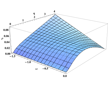
Figure 1: The induced energy density at an arbitrary fixed time as a function of $\omega$ and $q$ in the range of $-3/2<\omega<0$ and $0<q<4$ for the radiation dominated universe.

Also, we have plotted the induced energy density versus time in Figure $2$ for an allowed value of $\omega$ and $q$.

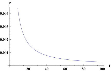
Figure 2: The evolution of the induced energy density in the radiation dominated universe with $\omega=-1.1$ and $q=2.5$.

By assuming the mentioned range that satisfies the WEC for the radiation dominated universe, relations (96)–(99) show that at $t=0$ the physical quantities $\rho$, $P_{\rm eff}$, $\Theta$, $\sigma^{2}$ and $V(\varphi)$ take infinite values. However, when $t\longrightarrow 0$ the BD scalar field takes finite values when $q\geq 1$ and diverges when $-1<q<1$. As in the limit $t\longrightarrow 0$, the spatial volume goes to zero and the expansion scalar tends to infinity, thus the evolution of universe starts with zero volume and the rate of the expansion is infinite. These results indicate that the model is in accordance with the big bang model. As $t$ increases, the expansion scalar decreases but the spatial volume increases, this shows that the rate of the expansion slows down by the time. When $t\longrightarrow\infty$, the spatial volume goes to infinity as well, whereas the other physical quantities, i.e. the expansion scalar, the scalar potential, the shear scalar, the induced energy density and the effective pressure tend to zero. However in this limit, the scalar field has two limits; it goes to infinity when $q>1$, while it becomes insignificant when $-1<q<1$. As the ratio $\sigma^{2}/\Theta^{2}$ does not depend on the time, the model, in general, does not approach isotropy for large values of $t$. Incidentally, the finite value of the integral

$$\int_{t_{0}}^{t}\frac{dt^{\prime}}{[\bar{V}(t^{\prime})]^{1/3}}=\frac{q+1}{q}\left[t^{\prime\frac{q}{q+1}}\right]_{t_{0}}^{t},$$ (100)

subject to $q\neq 0$, shows that there is a horizon in this model.

4.2.2 Stiff Fluid Distribution

The high energy density regime of the early universe is usually described with the stiff cosmological fluid. This kind of fluid, which is specified by the equation of state $P_{\rm eff}=\rho$, has been applied for the stellar and cosmological models with utter dense matter [53]. For the stiff fluid, by substituting $w=1$ into relations (89) and (90), one gains

$$p_{0}=\frac{2(q-2)}{q+1},\hskip 56.9055ptp_{4}=\frac{2-q}{q+1}$$ (101)

and

$$P_{\rm eff}=\rho=\frac{\kappa(2-q)}{24\pi(q+1)^{2}}\left[2q^{2}(\omega+1)-2q(4\omega+7)+(8\omega+11)\right]t^{-\frac{6}{q+1}}.$$ (102)

Substituting these values into relations (85), (86) and (74) gives the physical quantities as

$$\Theta={\frac{3}{(q+1)t}},$$ (103)

$$\sigma^{2}=\frac{-2q^{2}(\omega+1)+(8\omega+11)(q-1)}{(q+1)^{2}t^{2}}$$ (104)

and

$$V(\varphi)=\frac{4\kappa^{\frac{q+1}{q-2}}(\omega+1)(q-2)^{3}}{3(q+1)^{2}}\varphi^{\frac{3}{2-q}}.$$ (105)

For any value of $\omega>-1$ and $0<q<(4\omega+7-3\sqrt{2\omega+3})/[2(\omega+1)]$, the WEC is satisfied for the stiff fluid. Figure $3$ depicts the variation of the induced energy density at an arbitrary fixed time versus the BD coupling and the deceleration parameters. Also, in Figure $4$, the behavior of $\rho$ versus $q$ is plotted at an arbitrary fixed time and a constant value of the BD coupling parameter. The evolution of $\rho$, in this case, is similar to the one depicted in Figure $2$.

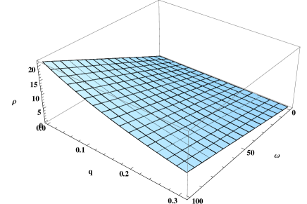
Figure 3: The induced energy density at an arbitrary fixed time versus $\omega$ and $q$ for the stiff fluid, where the BD coupling parameter is restricted to $-1<\omega<100$.

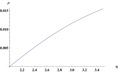
Figure 4: The induced energy density at an arbitrary fixed time versus $q$ with $\omega=0.5$ for the stiff fluid.

For this model, one observes that at $t=0$, the spatial volume is zero while the expansion scalar is infinite, which shows that the universe starts its evolution with zero volume at the beginning where the rate of the expansion is infinite. At the initial point $t=0$, the induced energy density, the effective pressure, the shear scalar and the induced scalar potential diverge. However, the BD scalar field has no initial singularity for $q\geq 2$ and diverges for $-1<q<2$. By increasing $t$, the expansion scalar decreases while the spatial volume increases, which indicates that the rate of the expansion decreases by the time. When $t$ goes to infinity the physical quantities $\rho$, $P_{\rm eff}$, $\sigma^{2}$, $\varphi$ (for $-1<q<2$), $V(\varphi)$ and $\Theta$ tend to zero, but the spatial volume and the BD scalar field (for $q>2$) become infinitely large. Thus, in the case of the stiff fluid, one has an empty universe for large values of the time. Again, as the ratio $\sigma^{2}/\Theta^{2}$ does not depend on the time, the model, in general, does not approach isotropy for large values of the cosmic time. The integral (100) also shows that there is a horizon for the stiff fluid distribution, and relation (101) indicates that, for $q>2$, its fifth dimension shrinks by the time.

5 Conclusions

As the BD theory is a modified version of general relativity, one can view the MBDT as a modified version of the IMT in which general relativity is replaced by the BD theory as the fundamental underlying theory. We purpose to investigate a generalized Bianchi type I anisotropic cosmology in $5D$ BD theory. Then, by employing the obtained formalism, we derive the induced scalar potential, the energy density and pressure of the induced–matter on any $4D$ hypersurface in the context of the MBDT. Hence, we probe the properties of the induced quantities for the specified cosmological model as the quantities fixed by the procedure rather than introduced priori by hand. Indeed, the core of the IMT idea, and hence the MBDT, for inducing $5D$ equations on any $4D$ hypersurface has been motivated to interpret the classical properties of $4D$ matter rather than solely accepting them. Hence, in the cosmological applications, what one obtains from vacuum $5D$ equations on any $4D$ hypersurface is actually the $5D$ quantities viewed as the ordinary matter.

Meanwhile, we illustrate that if a diagonalized metric, in the usual spatial dimensional isotropic case and in a gauge with a constant $g_{44}$, does not depend on the fifth coordinate while the scalar field does, it will lead, in general, to inconsistencies when the field equations are solved. Indeed, the induced scalar potential and the induced EMT vanish contrary to the results obtained in the literature. The exception case is $\omega=-1$ which is precisely the value predicted when the BD theory is derived as the low energy limit of some string theories. Also, there is a unique solution for when all the metric components (including the extra component, contrary to the above condition) depend only on the cosmic time while the scalar field is a function of the cosmic time and the extra coordinate.

At first and based on the usual spatial homogeneity, we assume, in general, that the scale factors of the specified $5D$ metric and the BD scalar field depend on the time, and also on the extra coordinate as separated variables in the power–law forms. Thus, we find five classes of solutions for the generalized Bianchi type I geometry in $5D$ space–time through which beside general investigations, for the sake of compactness, we probe only one interesting class of them that leads to a generalized Kasner cosmology in $5D$ BD theory. This class gives a generalized Kasner relations among the Kasner parameters. One important property of these relations occurs when the BD scalar field is a constant. That is, regardless of any specific value of the BD coupling parameter, the relations reduce to the corresponding relations in $5D$ general relativity, which in turn, give the $5D$ analogue of the well–known Kasner solution, as expected. Also, when the scale factors and the scalar field only depend on the time, in the particular case of spatial isotropy, the results are the same as the corresponding ones investigated before for the spatially flat FRW solutions in $5D$ BD theory.

We then derive the pressure and energy density of the specified induced–matter on any $4D$ hypersurface. These results indicate that one cannot consider it as a perfect fluid, however we discuss the effective $4D$ universe generated by the specified class of the solutions. The induced scalar potential is found to be either in the power–law or in the logarithmic form. However, in the particular case of constant scaler field and even when the scalar field only depends on the fifth dimension, the induced scalar potential, without loss of generality, vanishes. Then, the conservation law (which is supposed to be valid in this MBDT approach) has been checked explicitly for the derived induced EMT. Though, as the logarithmic form of the induced EMT has some difficulties in satisfying the WEC, we do not investigate it further.

We proceed our investigations for a few cosmological quantities where for simplicity (and somehow without loss of generality) we assume that the metric and the BD scalar field are only functions of the cosmic time. As usual in the Bianchi type I theories, we define a few (mean) parameters and important physical quantities, however, we have defined the effective pressure in a way to yield the conservation law in the case of isotropy. The other quantities under consideration are the spatial volume, the average scale factor, the mean Hubble parameter, the expansion scalar, the shear scalar and the deceleration parameter. First we obtain these quantities in terms of the generalized Kasner parameters. Then, we find that the induced EMT satisfies the barotropic equation of state $P_{\rm eff}=w\rho$, where $w$ is a function of the Kasner parameters. Also, the model indicates that a constant mean Hubble parameter is not allowed. Hence, by appealing to the special law of variation of the Hubble parameter, we assume that the deceleration parameter to be constant. And thus, we set the evolution of all the quantities with respect to the fixed deceleration parameter $q$, the state parameter $w$ and the BD coupling parameter. In general, the average scale factor indicates that any positive value of $q$ corresponds to a decelerating expanding universe, while the negative values of $q$, restricted to $-1<q<0$, yield accelerating expanding ones.

In the special case of a constant scalar field, regardless of any specific value of the BD coupling parameter, the BD theory reduces to general relativity, and we recover the generalized Kasner relations achieved before in the literature. The model, by satisfying the WEC, allows a shrinking extra dimension for a decelerating expanding universe which includes the radiation dominated and the matter dominated epoches that evolve the same as the corresponding ones of the flat FRW space–time in general relativity.

We then probe the quantities, in general case, versus $q$, $t$ and $\omega$ for the stiff fluid and the radiation dominated universe. The results show that in the both fluids, one has an expanding universe commenced with a big bang, and there is a horizon for each of them. The rate of expansion slows down by the time. Also, by applying the WEC, the allowed (or the well–behaved) ranges of the deceleration and the BD coupling parameters have been obtained for each of the fluids. The behavior of the quantities, in the very early universe and the very large time, has been discussed. In particular, the general behavior of the induced energy density, at an arbitrary fixed time and also its evolution, has been depicted in a few figures. The models give empty universes when the cosmic time goes to infinity. However, as the ratio $\sigma^{2}/\Theta^{2}$ does not depend on the cosmic time, the models, in general, do not approach isotropy for large values of the cosmic time.

As presented, the modified $4D$ BD theory with a non–vanishing scalar potential and the induced EMT is derived from the $5D$ BD equations with vacuum configuration, contrary to the standard $4D$ BD theory where the scalar potential introduced by hand. Note that, though for the Bianchi type I model interpreted by the standard approach, introduction of a scalar potential by hand may provide more freedom in obtaining interesting solutions, but we have investigated the response of the MBDT approach for the specified cosmological model.

6 Acknowledgment

We thank the Research Office of the Shahid Beheshti University for financial support.

References

- [1] T. Kaluza, Sitz. Preuss. Akad. Wiss. 33, 966 (1921).
- [2] O. Klein, Z. Phys. 37, 895 (1926).
- [3] P.S. Wesson and J. Ponce de Leon, J. Math. Phys. 33, 3883 (1992).
- [4] J.M. Overduin and P.S. Wesson, Phys. Rep. 283, 303 (1997).
- [5] P.S. Wesson, Space–Time–Matter, (World Scientific, Singapore, 1999).
- [6] P.S. Wesson, Five–Dimensional Physics (World Scientific, Singapore, 2006).
- [7] J.E. Lidsey, C. Romero, R. Tavakol and S. Rippl, Class. Quant. Grav. 14, 865 (1997).
- [8] F. Dahia and C. Romero “The embedding of the spacetime in five dimensions: an extension of Campbell–Magaard theorem”, gr-qc/0109076.
- [9] S.S. Seahra and P.S. Wesson, Class. Quant. Grav. 20, 1321 (2003).
- [10] S. Rippl, C. Romero and R. Tavakol, Class. Quant. Grav. 12, 2411 (1995).
- [11] P.S. Wesson, J. Ponce de Leon, H. Liu, B. Mashhoon, D. Kalligas, C.W.F. Everitt, A. Billyard, P. Lim and J.M. Overduin, Int. J. Mod. Phys. A 11, 3247 (1996).
- [12] P.S. Wesson, Astrophys. J. 436, 547 (1994).
- [13] N. Doroud, S.M. M. Rasouli and S. Jalalzadeh, Gen. Rel. Grav. 41, 2637 (2009).
- [14] A. Billyard and P.S. Wesson, Gen. Rel. Grav. 28, 129 (1996).
- [15] J.E.M. Aguilar, C. Romero and A. Barros, Gen. Rel. Grav. 40, 117 (2008).
- [16] J. Ponce de Leon, Class. Quant. Grav. 27, 095002 (2010).
- [17] J. Ponce de Leon, JCAP 03, 030 (2010).
- [18] A.F. Bahrehbakhsh, M. Farhoudi and H. Shojaie, Gen. Rel. Grav. 43, 847 (2011).
- [19] S.M. M. Rasouli and M. Farhoudi, “Modified Brans–Dicke theory in arbitrary dimensions”, work in progress.
- [20] E. Kasner, Am. J. Math. 48, 217 (1921).
- [21] S. Ram and D. K. Singh Astrophys. Space Sci. 95, 219 (1983).
- [22] D. Lorenz–Petzold, Phys. Rev. D 29, 2399 (1984).
- [23] P. Chauvet and J.L. Cervantes–Cota, Phys. Rev. D 52, 3416 (1995).
- [24] J.L. Cervantes–Cota and M. Nahmad, Gen. Rel. Grav. 33, 767 (2001).
- [25] A. Banerjee and N.O. Santos, Gen. Rel. Grav. 14, 559 (1982).
- [26] V.B. Johri and G.K. Goswami, Aust. J. Phys. 36, 235 (1983).
- [27] A. Banerjee, N. Banerjee and N.O. Santos, J. Math. Phys. 26, 3125 (1985).
- [28] P. Halpern, Phys. Rev. D 63, 024009 (2001).
- [29] J. Ponce de Leon and P.S. Wesson, Europhys. Lett. 84, 20007 (2008).
- [30] D.W. Chiou, Phys. Rev. D 76, 124037 (2007).
- [31] B. Vakili and H.R. Sepangi, Phys. Lett. B 651, 79 (2007).
- [32] C. Brans and R.H. Dicke, Phys. Rev. 124, 925 (1961).
- [33] P.G.O. Freund, Nucl. Phys. B 209, 146 (1982).
- [34] Y.M. Cho, Phys. Rev. Lett. 68, 3133 (1992).
- [35] J.D. Barrow, D. Kimberly and J. Magueijo, Class. Quant. Grav. 21, 4289 (2004).
- [36] N. Banerjee and D. Pavon, Phys. Rev. D 63, 043504 (2001).
- [37] A.E. Montenegro Jr and S. Carneiro, Class. Quant. Grav. 24, 313 (2007).
- [38] S. Sen and A.A. Sen, Phys. Rev. D 63, 124006 (2001).
- [39] L.-E. Qiang, Y.-G. Ma, M.-X. Han and D. Yu, Phys. Rev. D 71, 061501 (2005).
- [40] V. Faraoni, Cosmology in Scalar Tensor Gravity, (Kluiwer Academic Publishers, Netherlands, 2004).
- [41] D. Blaschke and M.P. Dabrowski “Conformal relativity versus Brans–Dicke and superstring theories”, hep-th/0407078.
- [42] C.M. Chen, T. Harko and M.K. Mak, Phys. Rev. D 64, 044013 (2001).
- [43] M. Heydari–Fard and H.R. Sepangi, Phys. Lett. B 649, 1 (2007).
- [44] M. Sharif and M. Farasat Shamir, Class. Quant. Grav. 26, 235020 (2009).
- [45] M. Sharif and M. Farasat Shamir, “Exact solutions of Bianchi–type I and V spacetimes in the theory of gravity”, gr-qc/1005.2798.
- [46] M.S. Bermann, Nuovo Cimento 74B, 182 (1983).
- [47] M.S. Bermann and F.M. Gomide, Gen. Rel. Grav. 20, 191 (1988).
- [48] D.R.K. Reddy, R.L. Naidu and V.U.M. Rao, Int. J. Theo. Phys. 46, 6 (2007).
- [49] C.P. Singh and S. Kumar, Astrophys. Space Sci. 310, 31 (2007).
- [50] A. Pradhan, H. Amirhashchi and B. Saha, “Bianchi type–I anisotropic dark energy models with constant deceleration parameter”, gr-qc/1010.1121.
- [51] W.L. Freedman and M.S. Turner, Rev. Mod. Phys. 75, 1433 (2003).
- [52] J. Ponce de Leon, Mod. Phys. Lett. A 16, 35 (2001).
- [53] Y.B. Zeldovich, Sov. Phys. JETP 14, 1143 (1962).