Application of the Kolmogorov-Smirnov test to CMB data:
Is the universe really weakly random?
A recent application of the Kolmogorov-Smirnov test to the WMAP 7 year W-band maps claims evidence that the CMB is “weakly random”, and that only 20% of the signal can be explained as a random Gaussian field. I here repeat this analysis, and in contrast to the original result find no evidence for deviation from the standard CDM model. Instead, the results of the original analysis are consistent with not properly taking into account the correlations of the CDM power spectrum.
Key Words.:
cosmic background radiation1 Introduction
In astronomical data analysis, it is often useful to be able to test whether a set of data points follows a given distribution or not. For example, many analysis techniques depend on instrument noise being Gaussian, and to avoid bias, one must check that this actually is the case. There are many different ways in which two distributions can differ, and correspondingly many different ways to test them for equality. The simplest ones, such as comparing the means or variances of the distributions, suffer from the problem that there are many ways in which distributions can differ that they cannot detect no matter how many samples are available. For example, samples from a uniform distribution can easily pass as Gaussian if one only considers the mean and variance.
The popular Kolmogorov-Smirnov test (K-S test) resolves this problem by considering the cumulative distribution functions (CDF) instead: Construct the empirical CDF of the data points and find its maximum absolute difference from the theoretical CDF. Due to the limited number of samples, the empirical CDF will be noisy, and will therefore be a random variable with its own CDF, which in the limit where the number of samples goes to infinity is given by
| (1) |
with
| (2) |
In contrast with the simplest tests, this test can detect any deviation in the distributions, but may require a large number of samples to do so, especially in the tails of the distribution.
Recently, a series of papers (Gurzadyan et al. 2011; Gurzadyan & Kocharyan 2008; Gurzadyan et al. 2010) has applied this test to WMAP’s cosmic microwave background (CMB) maps, resulting in the remarkable claim that the CMB is “weakly random”, with only 20% of the CMB signal behaving as one would expect from a random Gaussian field. This result went on to be used in a much discussed series of papers (Gurzadyan & Penrose 2010a, b, 2011) claiming a strong detection of concentric low-variance circles in the CMB, which was taken as evidence for Conformal Cyclic Cosmology. Other groups failed to significantly detect the circles (Wehus & Eriksen 2010; Moss et al. 2011; Hajian 2010). The difference in significance was due different CMB models: Wehus & Eriksen (2010); Moss et al. (2011); Hajian (2010) used realizations of the best-fit CDM power spectrum, while Gurzadyan & Penrose (2010b) used a “weakly random” CMB model.
Both in order to resolve this issue, and because a weakly random universe would be a strong blow against the CDM model in its own right, it is important to test this result.
2 Method
Before applying the K-S test, one must be aware of its limited area of validity: Equation (1) requires an infinite number of independently identically distributed samples, while CMB maps actually consist of a limited number of correlated samples. However, both the correlations and number of samples can be compensated for, as we shall see.
2.1 Application of the K-S test to correlated data
Though the K-S test is not immediately applicable to a correlated data set, it is possible to perform an equivalent test on a transformed set of samples. The question we are trying to answer with the K-S test is “Do the samples follow the theoretical distribution?”. The truth or falseness of this is preserved if we apply the same transformation to both the samples and the distribution we test them against, and to be able to use the K-S test, the logical transformation to use is a whitening transformation, which results in an independent, identical distribution for the samples. With original samples with covariance matrix , the whitened (uncorrelated with unit variance) samples are given by:
| (3) |
Thus, to test whether the data points , we can test the equivalent hypothesis .
In the case of CMB maps, both the data itself and the noise is expected to be Gaussian, so the obvious theoretical distribution here is , where the CMB signal covariance matrix is given by the two-point correlation function:
| (4) |
are the Legendre polynomials normalized to , and and are the direction vectors for pixel and in the disk. is the CDM angular power spectrum, while accounts for the beam and pixel window. is instrument dependent, but for the WMAP W-band CMB map we will use here, the noise is nearly diagonal, and given by the corresponding W-band RMS map.

2.2 Application of the K-S test with few samples
The other problem we need to account for is our finite number of samples. In this case equation (1) is only approximate. For most uses of the test, this approximation is good enough, especially when employing analytical expressions for improving the quality of the approximation for low numbers of samples (von Mises 1964). For example, when performing a single test to accept or reject a test distribution, a bias of a few percent in the confidence with which the hypothesis is rejected is not important.
However, when making statistics for a large number of such test results, such a bias may make the results ambiguous. Given a set of experiments with a corresponding set of maximum deviations , the corresponding probabilities should be uniformly distributed if the samples actually follow the theoretical distribution, and a histogram of should therefore be flat. Deviations from this indicate that the theoretical distribution does not accurately describe the samples. However, the approximate equation (1) also introduces a small non-uniformity in even if the samples actually do follow the distribution. To avoid the ambiguity this causes, we will instead compute a numerical correction function mapping the approximate to the true . 111 What we do here is essentially replacing the analytical Komolgorov distribution (equation (1)) with a numerical distribution. This could also be done without using the analytical distribution as a basis, at a small cost in clarity.
To build up the correction, we simulate a large number222 The number necessary depends on the level of accuracy desired. The noise in the estimate of propagates to the final results. To make this a subdominant noise contribution, the number of simulations should be at least as large as the number of actual experiments, preferably much higher. of experiments, each with the same number of samples as the actual data set, but drawn directly from the theoretical distribution. Thus, for these, should be uniform, with a CDF of . However, since equation (1) is inexact, for small numbers of samples, the actual CDF is . The mapping between the approximate and true is given by . Thus, for a limited number of samples
| (5) |
Figure 2 illustrates the correction function for simulations of 540 each. For this many samples, the correction is only of the order of 1%.

3 Does CDM fail the K-S test?
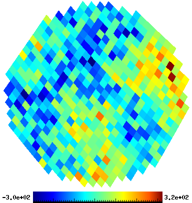
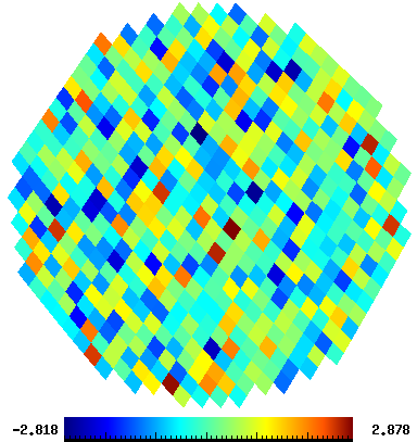
With this in hand we can finally apply the K-S test on CMB data. Following Gurzadyan et al. (2011), we randomly pick 10 000 disks with a radius of 1.5 degrees from the WMAP 7 year W-band map (Jarosik et al. 2011), with the region within 30 degrees from the galactic equator excluded. Each disk contains on average 540 pixels, which are whitened using equation (3). A typical disk before and after the whitening operation can be seen in Fig. 3. After whitening, the values should follow the distribution if our model is correct.
 |
 |
The histogram of resulting probabilities from of applying equation (5) to the hypothesis is shown in Fig. 4, together with the 68% and 95% intervals from 300 simulations. The data and simulations are consistent, and follow a uniform distribution as expected333 It should be noted that the histogram bins are not completely independent for two reasons: Firstly, some disks are going to overlap, meaning that the same samples enter into several different K-S tests, and secondly, while our transformation has made the samples within each disk independent, the correlation between different disks is still present.: The CMB map is fully consistent with CDM + WMAP noise as far as the K-S test is concerned.
This is dramatically different from the curve found by Gurzadyan et al. (2011), which was strongly biased towards low values. Low values of would mean that the empirical CDF of the samples matches the theoretical one too well, i.e. even better than samples drawn directly from the theoretical distribution.


What could cause Gurzadyan et al. to get results so different from ours? One way biasing low is by basing the parameters of your test distribution on the values themselves. However, even without doing this, it is possible to get low values if the values used in the K-S test are correlated. This is also consistent with the presentation given by Gurzadyan et al. (2011) who apparently applied the K-S test directly to the raw samples , or equivalently, that they model the pixel values as coming from a 1-dimensional distribution. To check this, I repeated the analysis, this time using the theoretical distribution , where and are the measured mean and variance of the samples in the disk. The result is also shown in Fig. 4. This time, the bias towards low values is clearly recreated.
It therefore seems likely that Gurzadyan et al.’s reported “weak randomness” is the result of not properly taking the CMB’s correlations into account. One is, of course, free to use whatever distribution one wants as the theoretical distribution in a K-S test, even a model where the CMB pixels are independently identically distributed, with no correlations at all. The problem lies in the interpretation of the test results. For Gurzadyan et al. (2011), the K-S test results are clearly not uniform, indicating that the chosen theoretical distribution has been disproven. However, Gurzadyan et al. then go on to create a set of simulations (linear combinations of 20% Gaussian and 80% static signal) that fail the test in the same way as the WMAP map does. But having two sets of samples fail the K-S test the same way does not prove that they have the same properties. It simply means that the chosen test distribution was a poor choice.
4 Kolmogorov maps
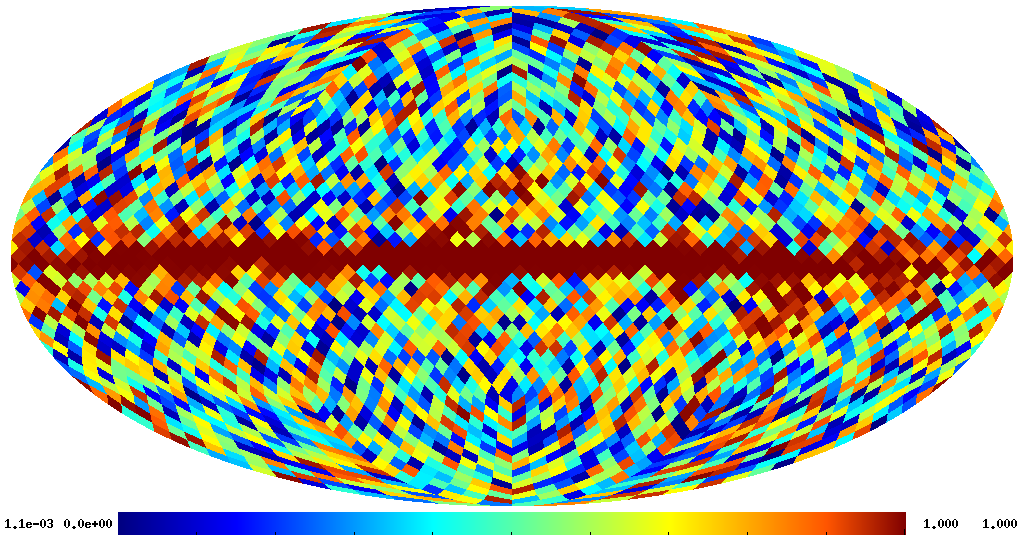
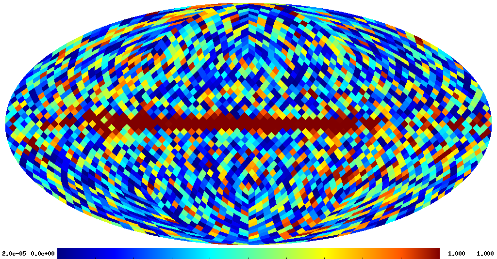
While Gurzadyan et al.’s Kolmogorov statistics are biased by not taking the correlations into account, the approach of making sky maps of K-S test results introduced in Gurzadyan et al. (2009) is still an interesting way to search for regions of the sky that do not follow the expected distribution. Making an unbiased Kolmogorov map straightforwardly follows the procedure in Sect. 3, with the main difference being the selection of pixels. Instead of randomly selecting disks, we now systematically go through nside 16 pixels, using the 1024 nside 512 subpixels inside each one as the samples. These are then tested against by whitening them via equation (3) and then comparing the whitened samples to .
The result is the nside 16 map of shown in Fig. 5. Regions that pass the test have a value uniformly distributed between 0 and 1, and we see that this applies to the CMB-dominated areas of the sky, while areas dominated by the galaxy fail the test as expected.
For comparison, Fig. 5 also includes the result of making the same map while ignoring correlations. In this case, the whole sky fails the test: The CMB-dominated areas are biased low, while the galaxy is biased high. This map is similar to the map in Gurzadyan et al. (2009), which is also too low outside the galaxy, and too high inside, which is, again, consistent with Gurzadyan et al. applying the K-S test directly to the raw samples.


5 Summary
The Kolmogorov-Smirnov test is a useful and general way of testing whether a data set follows a given distribution or not. However, it only applies to independently identically distributed samples. The CMB is strongly correlated, and thus not immediately compatible with the test. However, this can be resolved by the application of a whitening transformation, replacing the hypothesis with the equivalent . With this, we find that the CDM passes the K-S test. This is incompatible with the original analysis by Gurzadyan et al. (2011), which claimed detection of an unknown non-random component making up 80% of the CMB based on the CMB failing the K-S test there. It turns out that this analysis did not take the CMB correlations into account, which we confirm by producing the same failure of the K-S test when we skip the whitening step. When the correlations are handled properly, there is no need for a weakly random universe.
Acknowledgements.
The author would like to thank Hans Kristian Eriksen for useful discussion and comments.References
- Górski et al. (2005) Górski, K. M., Hivon, E., Banday, A. J., et al. 2005, ApJ, 622, 759, arXiv:astro-ph/0409513
- Gurzadyan et al. (2009) Gurzadyan, V. G., Allahverdyan, A. E., Ghahramanyan, T., et al. 2009, A&A, 497, 343, 0811.2732
- Gurzadyan et al. (2011) Gurzadyan, V. G., Allahverdyan, A. E., Ghahramanyan, T., et al. 2011, A&A, 525, L7+, 1011.3711
- Gurzadyan et al. (2010) Gurzadyan, V. G., Kashin, A. L., Khachatryan, H. G., et al. 2010, Europhysics Letters, 91, 19001, 1002.2155
- Gurzadyan & Kocharyan (2008) Gurzadyan, V. G. & Kocharyan, A. A. 2008, A&A, 492, L33, 0810.3289
- Gurzadyan & Penrose (2010a) Gurzadyan, V. G. & Penrose, R. 2010a, ArXiv e-prints, 1011.3706
- Gurzadyan & Penrose (2010b) Gurzadyan, V. G. & Penrose, R. 2010b, ArXiv e-prints, 1012.1486
- Gurzadyan & Penrose (2011) Gurzadyan, V. G. & Penrose, R. 2011, ArXiv e-prints, 1104.5675
- Hajian (2010) Hajian, A. 2010, ArXiv e-prints, 1012.1656
- Jarosik et al. (2011) Jarosik, N., Bennett, C. L., Dunkley, J., et al. 2011, ApJS, 192, 14, 1001.4744
- Moss et al. (2011) Moss, A., Scott, D., & Zibin, J. P. 2011, JCAP, 4, 33, 1012.1305
- von Mises (1964) von Mises, R. 1964, Mathematical Theory of Probability and Statistics, ed. von Mises, R.
- Wehus & Eriksen (2010) Wehus, I. K. & Eriksen, H. K. 2010, ArXiv e-prints, 1012.1268