Abstract

We construct a single scalar field model with tachyon field non-minimally coupled to itself, its derivative and to the curvature. We study the cosmological dynamics of the equation of state in this setup. While it is expected that in the case of single scalar field the crossing of the phantom divide line can not be realized [10], we show that incorporating quantum corrections namely, non-minimal derivative coupling of scalar field with curvature in our model, lead to phantom divide crossing.

PACS numbers: 95.36.+x, 98.80.-k, 04.50.kd
Keywords: Non-minimal derivative coupling; Tachyon field; Crossing of phantom divide.

1 Introduction

Recent cosmological observations have revealed that the present state of the universe is undergoing an accelerated expansion [1-4]. This acceleration is triggered by more than 70$\,{}_{\circ}/^{\circ}$ of dark energy. Dark energy (DE) has been one of most active field in modern cosmology [5]. The simplest candidate for DE is a tiny positive time-independent cosmological constant $\Lambda$. However, it has two problems: 1) fine tuning or why the cosmological constant is about 120 orders of magnitude smaller than its natural expectation (the Planck energy density), and 2) coincidence problem or why are we living in an epoch in which the DE density and the dust matter energy are comparable?
As a possible solution to these problems, many dynamical scalar field models of DE have been proposed. Quintessence, phantom, k-essence and tachyon scalar fields belong to these sort of DE models (for review see [6]).
In the other hand, various observational data such as SNe Ia Gold dataset [7] confirmed that the effective equation of state (EoS) parameter $\omega$ (the ratio of the effective pressure of the universe to the effective energy density of it) crosses $-1$, namely, the cosmological constant barrier, currently or in the past. It has been shown [8-11] that with a single fluid or a single minimally coupled scalar field it is impossible to realize EoS crossing $-1$ and one needs to introduce extra degree of freedom to the ordinary theories of these kinds.
A number of attempts to realize the crossing of the cosmological constant barrier are as follows: hybrid model which is composed of two scalar fields (quintessence and phantom) [11] or three scalar fields [12], scalar field model with non-linear kinetic terms [13] or a non-linear higher-derivative one [10], braneworld models [14], phantom coupled to dark matter with an appropriate coupling [15], string inspired models [16], non-local gravity [17], modified gravity models [18] and also non-minimally coupled scalar field models in which scalar field couples with scalar curvature, Gauss-Bonnet invariant or modified $f(R)$ gravity [19-21] (for a detailed review, see [22]). Crossing of the phantom divide can also be realized with single imperfect fluid [23] or by a constrained single degree of freedom dust like fluids [24].
Furthermore, non-minimal couplings are generated by quantum corrections to the scalar field theory and they are essential for the renormalizability of the scalar field theory in curved space (see [25] and references therein). One can extend the non-minimally coupled scalar tensor theories, allowing for non-minimal coupling between the derivatives of the scalar fields and the curvature [26]. A model with non-minimal derivative coupling was proposed in [26-28] and interesting cosmological behaviors of such a model in inflationary cosmology [29], quintessence and phantom cosmology [30, 31], asymptotic solutions and restrictions on the coupling parameter [32] have been widely studied in the literature. General non-minimal coupling of a scalar field and kinetic term to the curvature as a source of DE has been analyzed in [33]. Also, non-minimal coupling of modified gravity and kinetic part of Lagrangian of a massless scalar field has been investigated in [34]. It has been shown that inflation and late-time cosmic acceleration of the universe can be realized in such a model.
In this paper we consider an explicit coupling between the scalar field, the derivative of the scalar field and the curvature and study crossing of the $\omega=-1$ in such a model. We are interested in our analysis to the case of tachyon scalar field. The tachyon field in the world volume theory of the open string stretched between a D-brane and an anti-D-brane or a non-BPS D-brane plays the role of scalar field in the context of string theory [35]. What distinguishes the tachyon Lagrangian from the standard Klein-Gordan form for scalar field is that the tachyon action has a non-standard type namely, Dirac-Born-Infeld form [36]. Moreover, the tachyon potential is derived from string theory and should be satisfy some definite properties to describe tachyon condensation and other requirements in string theory. In summary, our motivation for investigating a model with non-minimal derivative coupling and tachyon scalar field is coming from a fundamental theory such as string/superstring theory and it may provide a possible approach to quantum gravity from a perturbative point of view [37-39].
An outline of the present work is as follows: In section 2 we introduce a model of DE in which the tachyon field plays the role of scalar field and the non-minimal coupling between scalar field, the time derivative of scalar field and Einstein tensor is also present in the action. Then we derive field equations as well as energy density and pressure of the model in order to study the EoS parameter behavior in section 3. We obtain the conditions required for $\omega$ crossing $-1$ and using numerical method, we will show that the model can realize the $\omega=-1$ crossing. Section 4 is devoted to our conclusions.

2 Field Equations

We consider the following Born-Infeld type action for tachyon field with non-minimal derivative coupling and also with itself,

$$S=\int d^{4}x\sqrt{-g}\Big{[}\frac{1}{2k^{2}}R-V(\phi)\sqrt{1+g^{\mu\nu}\partial_{\mu}\phi\partial^{\nu}\phi}+\xi f(\phi)G_{\mu\nu}\partial^{\mu}\phi\partial^{\nu}\phi\Big{]},$$ (1)

where $\kappa^{2}=8\pi G=\frac{1}{M_{Pl}^{2}}$ while $G$ is a bare gravitational constant and $M_{Pl}$ is a reduced Planck mass, $V(\phi)$ is the tachyon potential which is bounded and reaching its minimum asymptotically. $f(\phi)$ is a general function of the tachyon field $\phi$ and $\xi$ is coupling constant. The models of kind (1) with non-minimal coupling between derivatives of a scalar field and curvature are the extension of scalar-tensor theories. Such a non-minimal coupling may appear in some Kaluza-Klein theories [40, 41]. In Ref. [26], Amendola has considered a model with non-minimal coupling between derivative of scalar field and the Ricci scalar, $\xi R\partial_{\mu}\phi\partial^{\mu}\phi$, and by using generalized slow-roll approximations, he has obtained some inflationary solutions of this model.
A general model containing two derivative coupling terms $\xi_{1}R\partial_{\mu}\phi\partial^{\mu}\phi$ and $\xi_{2}R_{\mu\nu}\partial^{\mu}\phi\partial^{\nu}\phi$, has been studied in [27, 28]. It was shown in [30] that field equations of this theory are of third order in $g_{\mu\nu}$ and $\phi$, but in the special case where $-2\xi_{1}=\xi_{2}=\xi$ the order of equations are reduced to the second order. This particular choice of $\xi_{1}$ and $\xi_{2}$ leads to the non-minimal coupling between derivative of scalar field and the Einstein tensor, $\xi G_{\mu\nu}\partial^{\mu}\phi\partial^{\nu}\phi$. Sushkov in [30] has obtained the exact cosmological solutions of this theory and he has concluded that such a model is able to explain a quasi-de sitter phase as well as an exit from it without any fine-tuned potential.
Varying the action (1) with respect to metric tensor $g_{\mu\nu}$, leads to

$$G_{\mu\nu}=R_{\mu\nu}-\frac{1}{2}g_{\mu\nu}R=k^{2}\big{(}T_{\mu\nu}+T^{\prime}_{\mu\nu}\big{)},$$ (2)

where

$$T_{\mu\nu}=\nabla_{\mu}\phi\nabla_{\nu}\phi-\frac{1}{2}g_{\mu\nu}\big{(}\nabla\phi\big{)}^{2}-g_{\mu\nu}V(\phi),$$ (3)

and

$$T^{\prime}_{\mu\nu}=R\big{(}\nabla_{\mu}\phi\nabla_{\nu}\phi\big{)}-4\nabla_{\gamma}\phi\nabla_{(\mu}\phi R^{\gamma}_{\nu)}+G_{\mu\nu}\big{(}\nabla\phi\big{)}^{2}-2R_{\mu\nu\gamma\lambda}\nabla^{\gamma}\phi\nabla^{\lambda}\phi-2\nabla_{\mu}\nabla^{\gamma}\phi\nabla_{\nu}\nabla_{\gamma}\phi$$

$$+2\nabla_{\mu}\nabla_{\nu}\phi\hbox{$\hbox to0.0pt{$\sqcup$\hss}\sqcap$}\phi+g_{\mu\nu}\Big{(}\nabla^{\gamma}\nabla^{\lambda}\phi\nabla_{\gamma}\nabla_{\lambda}\phi-\big{(}\hbox{$\hbox to0.0pt{$\sqcup$\hss}\sqcap$}\phi\big{)}^{2}+2R^{\gamma\lambda}\nabla_{\gamma}\phi\nabla_{\lambda}\phi\Big{)}.$$ (4)

Scalar field equation of motion can be obtain by varying (1) with respect to $\phi$,

$$\nabla_{\mu}\Big{(}\frac{V(\phi)\nabla^{\mu}\phi}{u}\Big{)}-\frac{dV(\phi)}{d\phi}u-\xi f(\phi)G^{\mu\nu}\nabla_{\mu}\nabla_{\nu}\phi+\xi\frac{df(\phi)}{d\phi}G_{\mu\nu}\partial^{\mu}\phi\partial^{\nu}\phi=0,$$ (5)

where $u=\sqrt{1+\nabla_{\mu}\phi\nabla^{\mu}\phi}$.
For a spatially-flat Friedmann-Robertson-Walker (FRW) metric,

$$ds^{2}=-dt^{2}+a^{2}(t)(dr^{2}+r^{2}d\Omega^{2}),$$ (6)

the components of the Ricci tensor $R_{\mu\nu}$ and the Ricci scalar $R$ are given by

$$R_{00}=-3\big{(}\dot{H}+H^{2}\big{)},\,\,R_{ij}=a^{2}(t)\big{(}\dot{H}+3H^{2}\big{)}\delta_{ij},\,\,R=6\big{(}\dot{H}+2H^{2}\big{)},$$ (7)

where $H=\frac{\dot{a}(t)}{a(t)}$ is the Hubble parameter and $a(t)$ is the scale factor. The equation of motion of the scalar field for a homogeneous $\phi$ in FRW background (6) takes the following form

$$\frac{\ddot{\phi}}{1-\dot{\phi}^{2}}+3H\dot{\phi}+\frac{1}{V(\phi)}\frac{dV}{d\phi}$$

$$+\frac{\sqrt{1-\dot{\phi}^{2}}}{V(\phi)}\Bigg{(}3\xi H^{2}\Big{(}2f(\phi)\ddot{\phi}+\frac{df}{d\phi}\dot{\phi}^{2}\Big{)}+18\xi H^{3}f(\phi)\dot{\phi}+12\xi H\dot{H}f(\phi)\dot{\phi}\Bigg{)}=0.$$ (8)

The $(0,0)$ component and $(i,i)$ components of equation (2) correspond to energy density and pressure respectively,

$$\rho=\frac{V(\phi)}{\sqrt{1-\dot{\phi}^{2}}}+9\xi H^{2}f(\phi)\dot{\phi}^{2},$$ (9)

and

$$P=-V(\phi)\sqrt{1-\dot{\phi}^{2}}-\xi\big{(}3H^{2}+2\dot{H}\big{)}f(\phi)\dot{\phi}^{2}-2\xi H\Big{(}2f(\phi)\dot{\phi}\ddot{\phi}+\frac{df}{d\phi}\dot{\phi}^{3}\Big{)}.$$ (10)

Friedmann equation is also as follows,

$$H^{2}=\frac{\kappa^{2}}{3}\Big{(}\frac{V(\phi)}{\sqrt{1-\dot{\phi}^{2}}}+9\xi H^{2}f(\phi)\dot{\phi}^{2}\Big{)}.$$ (11)

Next, we want to investigate the effects of non-minimal derivative coupling on the cosmological evolution of EoS and see how the present model can be used to realize a crossing of phantom divide $\omega=-1$.

3 The $\omega=-1$ Crossing with Tachyon Field

To study the cosmological consequence of the present model we start with $\omega=\frac{P}{\rho}$. From the definition of EoS one can write $P+\rho=(1+\omega)\rho$. Using equations (9) and (10) we have the following expression,

$$\rho+P=\frac{V(\phi)\dot{\phi}^{2}}{\sqrt{1-\dot{\phi}^{2}}}+6\xi H^{2}f(\phi)\dot{\phi}^{2}-2\xi\dot{H}f(\phi)\dot{\phi}^{2}-2\xi H\Big{(}2f(\phi)\dot{\phi}\ddot{\phi}+\frac{df}{d\phi}\dot{\phi}^{3}\Big{)}.$$ (12)

The above equation must be zero when $\omega\rightarrow-1$. In order to achieve this requirement, we obtain two following possibilities,

$$\dot{\phi}=0,$$ (13)

or

$$\dot{\phi}\Big{(}\frac{V(\phi)}{\sqrt{1-\dot{\phi}^{2}}}+6\xi H^{2}f(\phi)-2\xi\dot{H}f(\phi)\Big{)}=2\xi H\Big{(}2f(\phi)\ddot{\phi}+\frac{df}{d\phi}\dot{\phi}^{2}\Big{)}.$$ (14)

Also, we have to check $\frac{d}{dt}(\rho+P)\neq 0$, when $\omega$ crosses over $-1$,

$$\frac{d}{dt}(\rho+P)=\frac{V(\phi)\dot{\phi}^{3}}{\sqrt{1-\dot{\phi}^{2}}}+\frac{2V(\phi)\dot{\phi}\ddot{\phi}}{\sqrt{1-\dot{\phi}^{2}}}+\frac{V(\phi)\dot{\phi}^{3}\ddot{\phi}}{\big{(}1-\dot{\phi}^{2}\big{)}^{\frac{3}{2}}}+2\xi\big{(}3H^{2}-2\dot{H}\big{)}\Big{(}2f(\phi)\dot{\phi}\ddot{\phi}+\frac{df}{d\phi}\dot{\phi}^{3}\Big{)}$$

$$+2\xi\big{(}6H\dot{H}-\ddot{H}\big{)}f(\phi)\dot{\phi}^{2}-2\xi H\Big{(}2f(\phi)\big{(}\dot{\phi}\dddot{\phi}+\ddot{\phi}^{2}\big{)}+5\frac{df}{d\phi}\dot{\phi}^{2}\ddot{\phi}+\frac{d^{2}f}{d\phi^{2}}\dot{\phi}^{4}\Big{)}.$$ (15)

If we assume the first case, namely $\dot{\phi}=0$, when $\omega$ crosses the phantom divide line, then equation (15) can be rewritten as the following form

$$\frac{d}{dt}(\rho+P)=-4\xi Hf(\phi)\ddot{\phi}^{2}.$$ (16)

It is clear from (16) that, the additional condition for having crossing of the phantom divide is $\Rightarrow\ddot{\phi}\neq 0$. One concludes from the above discussion that crossing of the phantom divide line in our model must be happen before reaching potential to its minimum, because at the minimum of the tachyon potential, we have $\ddot{\phi}=0$ and $\dot{\phi}\neq 0$ and this is a well known property of $V(\phi)$. Therefore when $\omega$ crosses $-1$ the tachyon field should continue to run away since $\ddot{\phi}\neq 0$.
The Authors of Ref. [42] have obtained the same result as ours. But in their proposal, they have inserted an extra term, $\phi\hbox{$\hbox to0.0pt{$\sqcup$\hss}\sqcap$}\phi$, in square root part of tachyon Lagrangian by hand. Note that in our model there is no extra term but we have included non-minimal coupling of tachyon field with its derivative and curvature due to quantum corrections.
In the next step we consider the second possibility in equation (14). Then equation (15) takes the following form

$$\frac{d}{dt}(\rho+P)=\frac{V(\phi)\dot{\phi}^{3}}{\sqrt{1-\dot{\phi}^{2}}}\Big{(}1+\frac{\ddot{\phi}}{1-\dot{\phi}^{2}}\Big{)}-2\xi\ddot{H}f(\phi)\dot{\phi}^{2}+6\xi H^{2}\frac{df}{d\phi}\dot{\phi}^{3}-2\xi H\Big{(}2f(\phi)\dot{\phi}\dddot{\phi}-2f(\phi)\ddot{\phi}^{2}$$

$$+3\frac{df}{d\phi}\dot{\phi}^{2}\ddot{\phi}+\frac{d^{2}f}{d\phi^{2}}\dot{\phi}^{4}\Big{)}.$$ (17)

We can see that even if $\ddot{\phi}=0$ and $\dddot{\phi}=0$, crossing $-1$ can be happen. In this case our results are the same as those obtained in Ref. [21] where tachyon field non-minimally coupled to Gauss-Bonnet invariant. So, it seems that in studying phantom divide crossing cosmology the non-minimal coupling of tachyon field with this derivative and Einstein tensor has the same effects as coupling of tachyon to Gauss-Bonnet invariant where crossing over $-1$ can be happen when tachyon potential reaches its minimum asymptotically.
In order to show that our model can realize crossing of $\omega=-1$ more clearly, we choose two specific tachyon potential and study evolution of EoS numerically. Figure 1 shows such a numerical calculations for $V(\phi)=V_{0}e^{-\alpha\phi^{2}}$ with constant $\alpha$. One can see that the model predicts crossing of $-1$ at redshift $z=1.65$. In figure 2 we have taken another tachyon potential $V(\phi)=\frac{V_{0}}{\phi^{2}}$. It has been shown that crossing of $\omega=-1$ can be realized in our model. In this case crossing of phantom divide takes place at $z=1.32$. Also we have used the function $f(\phi)=b\phi^{n}$ with constants $b$ and $n$.
Finally we note the following points: in our numerical calculations if we do not consider the non-minimal coupling of scalar field with itself, namely $f(\phi)=1$ [30, 31], then for $V(\phi)=V_{0}e^{-\alpha\phi^{2}}$ crossing of $\omega=-1$ can not be realized and for $V(\phi)=\frac{V_{0}}{\phi^{2}}$ the EoS will be a constant larger than $-1$ hence it doesn’t cross the phantom divide.

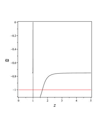
Figure 1: The plot of EoS parameter versus redshift $z$ for the potential $V(\phi)=V_{0}e^{-\alpha\phi^{2}}$, $\phi=\phi_{0}t$, $f(\phi)=b\phi^{n}$ and $H=\frac{h_{0}}{t}$, (with $\xi=10$, $b=1$, $n=8$, $V_{0}=4$, $h_{0}=100$, $\phi_{0}=0.5$ and $\alpha=5$). Crossing takes place at $z=1.65$.

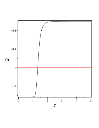
Figure 2: The plot of EoS parameter versus redshift $z$ for the potential $V(\phi)=\frac{V_{0}}{\phi^{2}}$, $\phi=\phi_{0}t$, $f(\phi)=b\phi^{n}$ and $H=\frac{h_{0}}{t}$, (with $\xi=10$, $b=1$, $n=8$, $V_{0}=4$, $h_{0}=100$ and $\phi_{0}=0.5$). Crossing takes place at $z=1.32$.

4 Conclusion

We have considered the gravitational theory of a scalar field with non-minimal derivative coupling to curvature and itself. We have studied cosmological evolution of EoS in this setup where tachyon field played the role of scalar field. We have shown that there are two possibilities to have phantom divide crossing to such a model. These possibilities are given by equations (13) and (14). By choosing the condition (13), we have concluded that the crossing over $-1$ must be happen before reaching tachyon potential to its minimum and this is the same result as that in [42]. In the other side if we consider the second possibility namely, the condition (14), it has been shown that the $\omega=-1$ crossing can be realized even if the potential goes to its minimum asymptotically. Our result in this case is the same as [21]. We have also investigated our model numerically and showed that the crossing of phantom divide occur for special potentials and coupling function. It may be interesting to consider different potentials and coupling functions in this setup.

References

- [1] A. G. Riess et al. [Supernova Search Team Collaboration], Astrophys. J. 607, 665 (2004) [astro-ph/0402512]; R. A. Knop et al., [Supernova Cosmology Project Collaboration], Astrophys. J. 598, 102 (2003) [astro-ph/0309368]; A. G. Riess et al. [Supernova Search Team Collaboration], Astron. J. 116, 1009 (1998) [astro-ph/9805201]; S. Perlmutter et al. [Supernova Cosmology Project Collaboration], Astrophys. J. 517, 565 (1999) [astro-ph/9812133].
- [2] C. L. Bennett et al., Astrophys. J. Suppl. 148, 1 (2003) [astro-ph/0302207]; D. N. Spergel et al., Astrophys. J. Suppl. 148, 175 (2003) [astro-ph/0302209].
- [3] M. Tegmark et al. [SDSS Collaboration], Phys. Rev. D 69, 103501 (2004) [astro-ph/0310723]; M. Tegmark et al. [SDSS Collaboration], Astrophys. J. 606, 702 (2004) [astro-ph/0310725]; U. Seljak et al., Phys. Rev. D 71, 103515 (2005) [astro-ph/0407372]; J. K. Adelman-McCarthy et al. [SDSS Collaboration], [astro-ph/0507711]; K. Abazajian et al. [SDSS Collaboration], [astro-ph/0410239]; [astro-ph/0403325]; [astro-ph/0305492].
- [4] S. W. Allen, R. W. Schmidt, H. Ebeling, A. C. Fabian and L. van Speybroeck, Mon. Not. Roy. Astron. Soc. 353, 457 (2004) [astro-ph/0405340].
- [5] P. J. E. Peebles and B. Ratra, Rev. Mod. Phys. 75, 559 (2003)[astro-ph/0207347]; S. M. Carroll, [astro-ph/0310342]; R. Bean, S. Carroll and M. Trodden, [astro-ph/0510059]; V. Sahni and A. A. Starobinsky, Int. J. Mod. Phys. D 9, 373 (2000) [astro-ph/9904398]; S. M. Carroll, Living Rev. Rel. 4, 1 (2001) [astro-ph/0004075]; T. Padmanabhan, Curr. Sci. 88, 1057 (2005) [astro-ph/0411044]; S. Weinberg, Rev. Mod. Phys. 61, 1 (1989); S. Nobbenhuis, [gr-qc/0411093].
- [6] T. Padmanabhan, Phys. Repts. 380, 235 (2003); E. J. Copeland, M. Sami and S. Tsujikawa, Int. J. Mod. Phys. D 15, 1753 (2006); M. Li, X.-D. Li, S. Wang and Y. Wang, [astro-ph. CO/1103.5870].
- [7] S. Nojiri and S. D. Odintsov, [astro-ph/0801.4843]; [hep-th/0807.0685]; T. P. Sotiriou and V. Faraoni, [gr-qc/0805.1726]; F. S. N. Lobo, [gr-qc/0807.1640]; S. Capozziello and M. Francaviglia, Gen. Rel. Grav. 40, 357 (2008).
- [8] G.-B. Zhao, J.-Q. Xia, M. Li, B. Feng and X. Zhang, Phys. Rev. D 72, 123515 (2005).
- [9] R. R. Caldwell, M. Doran, Phys. Rev. D 72, 043527 (2005); W. Hu, Phys. Rev. D 71, 047301 (2005).
- [10] A. Vikman, Phys. Rev. D 71, 023515 (2005).
- [11] B. Feng, X. Wang and X. Zhang, Phys. Lett. B 607, 35 (2005).
- [12] L. P. Chimento, M. Forte, R. Lazkoz and M. G. Richarte, Phys.Rev.D 79, 043502 (2009).
- [13] S. Nojiri, S. D. Odintsov and M. Sasaki, Phys. Rev. D 71, 123509 (2005) [hep-th/0504052]; M. Sami, A. Toporensky, P. V. Tretjakov and S. Tsujikawa, Phys. Lett. B 619, 193 (2005); B. M. Leith and I. P. Neupane, JCAP 0705, 019 (2007); S. Nojiri, S. D. Odintsov and M. Sami, Phys. Rev. D 74, 046004 (2006) [hep-th/0605039]; T. Koivisto and D. F. Mota, Phys. Lett. B 644, 104 (2007); M. R. Setare and E. N. Saridakis, Phys. Lett. B 670, 1 (2008); A. K. Sanyal, [astro-ph/0710.2450].
- [14] C. Deffayet, G. R. Dvali and G. Gabadadze, Phys. Rev. D 65, 044023 (2002) [astro-ph/0105068]; M. R. Setare, Phys. Lett. B 642, 421, (2006).
- [15] M. Z. Li, B. Feng and X. m. Zhang, JCAP 0512, 002 (2005) [hep-ph/0503268].
- [16] M. Cataldo and L. P. Chimento, [astro-ph/0710.4306].
- [17] B. McInnes, Nucl. Phys. B 718, 55 (2005); R. G. Cai, H. S. Zhang and A. Wang, Commun. Theor. Phys. 44, 948 (2005); R. G. Cai, Y. g. Gong and B. Wang, JCAP 0603, 006 (2006); I. Y. Aref eva, A. S. Koshelev and S. Y. Vernov, Phys. Rev. D 72, 064017 (2005); G. Kofinas, G. Panotopoulos and T. N. Tomaras, JHEP 0601, 107 (2006); I. Y. Aref eva and A. S. Koshelev, ibid. 0702, 041 (2007); L. P. Chimento, R. Lazkoz, R. Maartens and I. Quiros, JCAP 0609, 004 (2006); P. S. Apostolopoulos and N. Tetradis, Phys. Rev. D 74, 064021 (2006); S. F. Wu, A. Chatrabhuti, G. H. Yang and P. M. Zhang, ibid. 659, 45 (2008); J. Sadeghi, M. R. Setare, A. Banijamali and F. Milani, Phys. Lett. B 662, 92 (2008).
- [18] K. Bamba, C. -Q. Geng, S. Nojiri and S. D. Odintsov, Phys. Rev. D 79, 083014 (2009).
- [19] R. R. Caldwell, Phys. Lett. B 545, 23 (2002); S. Nojiri and S. D. Odintsov, Phys. Lett. B 562, 147 (2003) [hep-th/0303117].
- [20] L. Perivolaropoulos, JCAP 0510, 001 (2005).
- [21] J. Sadeghi, M. R. setare, A. Banijamali and F. Milani, Phys. Rev. D 79, 123003 (2009).
- [22] T. Padmanabhan, Phys. Rept. 380, 235 (2003).
- [23] C. Deffayet, O. Pujolas, I. Sawicki and A. Vikman, JCAP 1010, 026 (2010); O. Pujolas, I. Sawicki and A. Vikman, [hep-th/1103.5360].
- [24] E. A. Lim, I. Sawicki and A. Vikman, JCAP 1005, 012 (2010).
- [25] V. Faraoni, Phys. Rev. D 62, 023504 (2000).
- [26] L. Amendola, Phys. Lett. B 301, 175 (1993).
- [27] S. Capozziello and G. Lambiase, Gen. Rel. Grav. 31, 1005 (1999) [gr-qc/9901051].
- [28] S. Capozziello, G. Lambiase and H.-J.Schmidt, Annalen Phys. 9, 39 (2000) [gr-qc/9906051].
- [29] C. Germani and A. Kehagias, [hep-ph/1003.2635].
- [30] S. V. Sushkov, Phys. Rev. D 80, 103505 (2009).
- [31] E. N. Saridakis and S. V. Sushkov, Phys. Rev. D 81, 083510 (2010); H. M. Sadjadi, Phys. Rev. D 83 107301 (2011).
- [32] S. F. Daniel and R. R. Caldwell, Class. Quant. Grav 24, 5573 (2007).
- [33] L. N. Granda and W. Cardona, JCAP 07, 021 (2010).
- [34] S. Nojiri, S. D. Odintsov and P. V. Tretyakov, Prog. Theor. Phys. Suppl. 172, 81-89 (2008).
- [35] S. Alexander, Phys. Rev. D 65, 023507 (2002) [hep-th/0105032]; A. Mazumdar, S. Panda and A. Perez-Lorenzana, Nucl. Phys. B 614, 101 (2001), [hep-ph/0107058]; G. Gibbons, Phys. Lett. B 537, 1 (2002), [hep-th/0204008].
- [36] A. Sen, JHEP 9910, 008 (1999), [hep-th/9909062]; E. Bergshoeff, M. de Roo, T. de Wit, E. Eyras and S. Panda, JHEP 0005, 009 (2000) [hep-th/0003221]; J. Kluson, Phys. Rev. D 62, 126003 (2000) [hep-th/0004106].
- [37] M. B. Green, J. H. Schwarz and E. Witten, Superstring Theory, Cambridge University Press (1987).
- [38] H. Liu and A. A. Tseytlin, Nucl. Phys. B 533, 88 (1998) [hep-th/9804083].
- [39] S. Nojiri and S. D. Odintsov, Phys. Lett. B 444, 92 (1998) [hep-th/9810008].
- [40] Q. Shafi and C. Wetterich, Phys. Lett. B 152, 51 (1985).
- [41] Q. Shafi and C. Wetterich, Nucl. Phys. B 289, 787 (1987).
- [42] Y. f. Cai, M. z. Li, J. X. Lu, Y. S. Piao, T. t. Qiu and X. m. Zhang, Phys. Lett. B 651, 1 (2007).