One-Point Functions of the Integrable Spin-1 XXZ Chain

Quantum Group $\bm{U_{q}(sl(2))}$ Symmetry
and Explicit Evaluation of the One-Point Functions
of the Integrable Spin-1 XXZ Chain

Tetsuo DEGUCHI and Jun SATO

T. Deguchi and J. Sato

Department of Physics, Graduate School of Humanities and Sciences, Ochanomizu University
2-1-1 Ohtsuka, Bunkyo-ku, Tokyo 112-8610, Japan deguchi@phys.ocha.ac.jp, jsato@sofia.phys.ocha.ac.jp

Received October 29, 2010, in final form May 26, 2011; Published online June 10, 2011

We show some symmetry relations among the correlation functions of the integrable higher-spin XXX and XXZ spin chains, where we explicitly evaluate the multiple integrals representing the one-point functions in the spin-1 case. We review the multiple-integral representations of correlation functions for the integrable higher-spin XXZ chains derived in a region of the massless regime including the anti-ferromagnetic point. Here we make use of the gauge transformations between the symmetric and asymmetric $R$-matrices, which correspond to the principal and homogeneous gradings, respectively, and we send the inhomogeneous parameters to the set of complete $2s$-strings. We also give a numerical support for the analytical expression of the one-point functions in the spin-1 case.

quantum group; integrable higher-spin XXZ chain; correlation function; multiple integral; fusion method; Bethe ansatz; one-point function

82B23

1 Introduction

The correlation functions of the spin-1/2 XXZ spin chain has attracted much interest during the last decades in mathematical physics, and several nontrivial results such as their multiple-integral representations have been obtained explicitly [2, 3, 4]. The Hamiltonian of the XXZ spin chain under the periodic boundary conditions (P.B.C.) is given by

$${\cal H}_{\rm XXZ}=\sum_{j=1}^{L}\left(\sigma_{j}^{X}\sigma_{j+1}^{X}+\sigma_{j}^{Y}\sigma_{j+1}^{Y}+\Delta\sigma_{j}^{Z}\sigma_{j+1}^{Z}\right).$$

Here $\sigma_{j}^{a}$ ($a=X,Y,Z$) are the Pauli matrices defined on the $j$th site and $\Delta$ denotes the anisotropy of the exchange coupling. The P.B.C. are given by $\sigma_{L+1}^{a}=\sigma_{1}^{a}$ for $a=X,Y,Z$.

The XXZ Hamiltonian shows the quantum phase transition: the ground state of the XXZ spin chain depends on $\Delta$. For $|\Delta|>1$ the low-lying excitation spectrum at the ground state has a gap, while for $|\Delta|\leq 1$ it has no gap. Here we remark that the quantum phase transition that we have discussed is associated with the behavior of the XXZ spin chain in the thermodynamic limit: $L\rightarrow\infty$. In terms of the $q$ parameter of the quantum group $U_{q}(sl_{2})$, we express $\Delta$ as follows

$$\Delta={\frac{1}{2}}\left(q+q^{-1}\right).$$

It is often convenient to define parameters $\eta$ and $\zeta$ by $q=\exp\eta$ with $\eta=i\zeta$. Here we have $\Delta=\cosh\eta=\cos\zeta$. In the massive regime $\Delta>1$, we set $\eta>0$. In the massless regime $-1<\Delta\leq 1$, we set $\eta={\rm i}\zeta$ where $\zeta$ satisfies $0\leq\zeta<\pi$. Here, the XXX limit is given by $\eta\to+0$ or $\zeta\to+0$. Here we remark that the XXZ Hamiltonian can be derived from the $R$-matrix of the affine quantum group with $q$ parameter, $U_{q}(\widehat{sl_{2}})$: we derive the $R$-matrix by solving the intertwining relations, construct the XXZ transfer matrix from the product of the $R$ matrices, and then we derive the XXZ Hamiltonian by taking the logarithmic derivative of the XXZ transfer matrix. Thus, the $q$ parameter of the affine quantum group is related to the ground state of the XXZ spin chain through $\Delta$.

The multiple-integral representations of the XXZ correlation functions were derived for the first time by making use of the $q$-vertex operators through the affine quantum-group symmetry in the massive regime for the infinite lattice at zero temperature [5, 3]. In the massless regime they were derived by solving the $q$-KZ equations [6, 7]. Making use of the algebraic Bethe-ansatz techniques [8, 2, 9, 10, 11], the multiple-integral representations were derived for the spin-1/2 XXZ correlation functions under a non-zero magnetic field [12]. Here, they are derived through the thermodynamic limit after calculating the scalar product for a finite chain. The multiple-integral representations were extended into those at finite temperatures [13], and even for a large finite chain [14]. Interestingly, they are factorized in terms of single integrals [15]. We should remark that the multiple-integral representations of the dynamical correlation functions were also obtained under finite-temperatures [16]. Furthermore, the asymptotic expansion of a correlation function of the XXZ model has been systematically discussed [17]. Thus, the exact study of the XXZ correlation functions should play an important role not only in the mathematical physics of integrable models but also in many areas of theoretical physics.

Recently, the form factors of the integrable higher-spin XXX spin chains and the multiple-integral representations of correlation functions for the integrable higher-spin XXX and XXZ chains have been derived by the algebraic Bethe-ansatz method [18, 19, 20, 21, 22] (see also [23]). The spin-1 XXZ Hamiltonian under the P.B.C. is given by the following [24]:

$${\cal H}_{\text{spin-1 XXZ}}=J\sum_{j=1}^{N_{s}}\bigg{\{}{\vec{S}}_{j}\cdot{\vec{S}}_{j+1}-({\vec{S}}_{j}\cdot{\vec{S}}_{j+1})^{2}-{\frac{1}{2}}(q-q^{-1})^{2}[S_{j}^{z}S_{j+1}^{z}-(S_{j}^{z}S_{j+1}^{z})^{2}+2(S_{j}^{z})^{2}]$$

$$\qquad{}-(q+q^{-1}-2)[(S_{j}^{x}S_{j+1}^{x}+S_{j}^{y}S_{j+1}^{y})S_{j}^{z}S_{j+1}^{z}+S_{j}^{z}S_{j+1}^{z}(S_{j}^{x}S_{j+1}^{x}+S_{j}^{y}S_{j+1}^{y})\bigg{\}}.$$ (1.1)

Furthermore, the multiple-integral representations have been obtained for the correlation functions at finite temperature of the integrable spin-1 XXX chain [25]. The solvable higher-spin generalizations of the XXX and XXZ spin chains have been derived by the fusion method in several references [26, 27, 28, 29, 30, 31, 32, 33]. In the region: $0\leq\zeta<\pi/2s$, the spin-$s$ ground-state should be given by a set of string solutions [34, 35]. Furthermore, the critical behavior should be given by the SU(2) WZWN model of level $k=2s$ with central charge $c=3s/(s+1)$ [36, 37, 38, 39, 40, 41, 42, 43, 44, 45, 32, 46, 47, 48]. For the integrable higher-spin XXZ spin chain correlation functions have been discussed in the massive regime by the method of $q$-vertex operators [49, 50, 51, 24, 52, 53].

The purpose of this paper is to show some symmetry relations among the correlation functions of the integrable spin-$s$ XXZ spin chain by explicitly calculating the multiple-integral representations for the spin-1 one-point functions. Associated with the quantum group $U_{q}(sl(2))$ symmetry, there are several relations among the expectation values of products of the matrix elements of the monodromy matrices. For the spin-1 case, we confirm some of them by evaluating the multiple integrals analytically and explicitly. Here we should remark that the derivation of the multiple-integral representations for the spin-$s$ XXZ correlation functions given in the previous papers [20, 21, 22] was not completely correct: the application of the formulas of the quantum inverse-scattering problem was not valid [54, 55]. We thus review the revised derivation [54, 55] in the paper. The spin-$s$ correlation function of an arbitrary entry is now expressed in terms of a sum of multiple integrals, not as a single multiple integral. Furthermore, we show numerical results which confirm the analytical expressions of the spin-1 one-point functions.

Let us express by $\langle E^{00}\rangle$, $\langle E^{11}\rangle$ and $\langle E^{22}\rangle$, the expectation values of $S_{1}^{Z}=1$, $S_{1}^{Z}=0$ and $S_{1}^{Z}=-1$, respectively, where $S_{1}^{Z}$ denotes the $Z$-component of the spin operator defined on the first site. Then, we have the following:

$$\langle E^{22}\rangle=\langle E^{00}\rangle=\frac{\zeta-\sin\zeta\cos\zeta}{2\zeta\sin^{2}\zeta},\qquad\langle E^{11}\rangle=\frac{\cos\zeta(\sin\zeta-\zeta\cos\zeta)}{\zeta\sin^{2}\zeta}.$$

We shall show the derivation of $\langle E^{00}\rangle$, $\langle E^{11}\rangle$ and $\langle E^{22}\rangle$, in detail. Here we remark that the expressions of $\langle E^{22}\rangle$, the emptiness formation probability, and $\langle E^{11}\rangle$ have been reported in [21] without an explicit derivation. In fact, although the derivation was not completely correct, the expressions of the spin-1 one-point functions are correct [54, 55]. Here, the quantum group symmetry as well as the spin inversion symmetry play an important role, as we shall show explicitly in the present paper.

It is nontrivial to evaluate the multiple integral representations of the XXX and XXZ models analytically or even numerically. Let us now return to the spin-1/2 case. Boos and Korepin have analytically evaluated the emptiness formation probability $P(n)$ of the XXX spin chain for up to $n=4$ successive lattice sites [56]. Performing explicit evaluation of the multiple integrals, they successfully reproduced Takahashi’s result that was obtained through the one-dimensional Hubbard model [57]. The method was applied to all the density matrix elements for up to $n=4$ successive lattice sites in the XXX chain [58] and also in the XXZ chain [59, 60, 61]. Furthermore, the algebraic method to obtain the correlation functions of the XXX chain based on the $q$KZ equation has been developed [62] and the two-point functions up to $n=8$ have been obtained so far [63, 64, 65, 66]. At the special anisotropy $\Delta=1/2$, some further results have been shown for the correlation functions through explicit evaluation [67, 68, 69, 70].

The paper consists of the following. In Section 2 we review the Hermitian elementary matrices [21], and give the basis vectors and their conjugate vectors in the spin-1 case as an illustrative example. We also show a formula for expressing higher-spin local operators in terms of spin-1/2 local operators in the spin-1 case, which plays a central role in the revised method [54, 55]. In Section 3 we summarize the notation of the fusion transfer matrices and the quantum inverse scattering problem for the spin-$s$ operators. For an illustration, in Section 4, we show some relations among the expectation values of the Hermitian elementary matrices in the spin-1 XXX case and then in the spin-1 XXZ case. In particular, we show the spin inversion symmetry. We also show the transformation which maps the basis vectors of the spin-1 representation $V^{(2)}$ constructed in the tensor product of the spin-1/2 representations $V^{(1)}\otimes V^{(1)}$ to the basis of the three-dimensional vector space ${\bf C}^{3}$. The former basis is related to the fusion method, while the spin-1 XXZ Hamiltonian (1.1) is formulated in terms of the latter basis. In Section 5, we review the revised multiple-integral representations of correlation functions for the integrable spin-$s$ XXZ spin chain [54, 55]. Here we remark that necessary corrections to the previous papers [20] and [21] are listed in references [20] and [21] of the paper [55], respectively. In Section 6, we explicitly calculate the multiple integrals of the one-point functions for the spin-1 XXZ spin chain for a region in the massless regime. We show some details of the calculation such as shifting the integral paths. In Section 7 we show that the numerical estimates of the spin-1 one-point functions obtained through exact diagonalization of the spin-1 XXZ Hamiltonian (1.1) are consistent with the analytical expressions of the spin-1 one-point functions. Thus, we shall conclude that the analytical result of the spin-1 one-point functions should be valid.

2 The quantum group invariance

We construct the basis vectors of the finite-dimensional spin-$\ell/2$ representation of the quantum group $U_{q}(sl_{2})$ in the tensor product space of the spin-1/2 representations, and introduce their conjugate vectors. In terms of the basis and conjugate basis vectors we formulate the spin-$\ell/2$ elementary matrices which have only one nonzero element 1 with respect to entries of the basis and conjugate basis vectors. We then illustrate an important formula for reducing the spin-$\ell/2$ elementary matrices into a sum of products of the spin-1/2 elementary operators.

2.1 Quantum group $\bm{U_{q}(sl_{2})}$

Let us introduce the quantum group $U_{q}(sl_{2})$ in order to formulate not only the $R$-matrix of the integrable spin-$s$ XXZ spin chain algebraically but also the higher-spin elementary matrices, by which we introduce correlation functions. Here we remark that the correlation functions of the spin-$s$ XXZ spin chains are given by the expectation values of products of the higher-spin elementary matrices at zero temperature.

The quantum algebra $U_{q}(sl_{2})$ is an associative algebra over ${\bf C}$ generated by $X^{\pm}$, $K^{\pm}$ with the following relations [71, 72, 73]:

$$KK^{-1}=K^{-1}K=1,\qquad KX^{\pm}K^{-1}=q^{\pm 2}X^{\pm},\qquad{[}X^{+},X^{-}{]}={\frac{K-K^{-1}}{q-q^{-1}}}.$$

The algebra $U_{q}(sl_{2})$ is also a Hopf algebra over ${\bf C}$ with comultiplication

$$\Delta(X^{+})=X^{+}\otimes 1+K\otimes X^{+},\qquad\Delta(X^{-})=X^{-}\otimes K^{-1}+1\otimes X^{-},\qquad\Delta(K)=K\otimes K,$$

and antipode: $S(K)=K^{-1}$, $S(X^{+})=-K^{-1}X^{+}$, $S(X^{-})=-X^{-}K$, and coproduct: $\epsilon(X^{\pm})=0$ and $\epsilon(K)=1$.

2.2 Basis vectors of spin-$\bm{\ell/2}$ representation of $\bm{U_{q}(sl_{2})}$

We introduce the $q$-integer for an integer $n$ by $[n]_{q}=(q^{n}-q^{-n})/(q-q^{-1})$. We define the $q$-factorial $[n]_{q}!$ for integers $n$ by

$$[n]_{q}!=[n]_{q}[n-1]_{q}\cdots[1]_{q}.$$

For integers $m$ and $n$ satisfying $m\geq n\geq 0$ we define the $q$-binomial coefficients as follows

$$\left[\begin{matrix}m\\ n\end{matrix}\right]_{q}={\frac{[m]_{q}!}{[m-n]_{q}![n]_{q}!}}.$$

Let us denote by $|\alpha\rangle$ for $\alpha=0,1$, the basis vectors of the spin-1/2 representation $V^{(1)}$. Here we remark that 0 and 1 correspond to $\uparrow$ and $\downarrow$, respectively. In the $\ell$th tensor product space $(V^{(1)})^{\otimes\ell}$ we construct the basis vectors of the $(\ell+1)$-dimensional irreducible representation of $U_{q}(sl_{2})$, $||\ell,n\rangle$ for $n=0,1,\ldots,\ell$, as follows. We define the highest weight vector $||\ell,0\rangle$ by

$$||\ell,0\rangle=|0\rangle_{1}\otimes|0\rangle_{2}\otimes\cdots\otimes|0\rangle_{\ell}.$$

Here $|\alpha\rangle_{j}$ for $\alpha=0,1$, denote the basis vectors of the spin-1/2 representation defined on the $j$th position in the tensor product $(V^{(1)})^{\otimes\ell}$. We define $||\ell,n\rangle$ for $n\geq 1$ and evaluate them as follows [20]

$$||\ell,n\rangle=\big{(}\Delta^{(\ell-1)}(X^{-})\big{)}^{n}||\ell,0\rangle{\frac{1}{[n]_{q}!}}=\sum_{1\leq i_{1}<\cdots<i_{n}\leq\ell}\sigma_{i_{1}}^{-}\cdots\sigma_{i_{n}}^{-}|0\rangle q^{i_{1}+i_{2}+\cdots+i_{n}-n\ell+n(n-1)/2}.$$

Here $\sigma_{j}^{-}$ denotes the Pauli spin operator $\sigma^{-}$ acting on the $j$th component of the tensor product $(V^{(1)})^{\otimes\ell}$: we have $\sigma_{j}^{-}=I^{\otimes(j-1)}\otimes\sigma^{-}\otimes I^{\otimes(\ell-j)}$. We define the conjugate vectors explicitly by the following:

$$\langle\ell,n||=\left[\begin{matrix}\ell\\ n\end{matrix}\right]_{q}^{-1}q^{n(\ell-n)}\sum_{1\leq i_{1}<\cdots<i_{n}\leq\ell}\langle 0|\sigma_{i_{1}}^{+}\cdots\sigma_{i_{n}}^{+}q^{i_{1}+\cdots+i_{n}-n\ell+n(n-1)/2}.$$

It is easy to show the normalization conditions [20]: $\langle\ell,n||\,||\ell,n\rangle=1$. Let us define $F(\ell,n)$ by

$$F(\ell,n)=\left[\begin{matrix}\ell\\ n\end{matrix}\right]_{q}q^{-n(\ell-n)}.$$

We have $\left(||\ell,n\rangle\right)^{t}||\ell,n\rangle=F(\ell,n)$, and hence $\langle\ell,n||=\left(||\ell,n\rangle\right)^{t}/F(\ell,n)$. Here the superscript $t$ denotes the matrix transposition.

In the massive regime where $q=\exp\eta$ with real $\eta$, conjugate vectors $\langle\ell,n||$ are also Hermitian conjugate to vectors $||\ell,n\rangle$.

2.3 Affine quantum group $\bm{U_{q}(\widehat{sl_{2}})}$

In order to define the $R$-matrix in terms of algebraic relations we now introduce the affine quantum group $U_{q}(\widehat{sl_{2}})$. It is an infinite-dimensional algebra generalizing the quantum group $U_{q}(sl_{2})$.

The algebra $U_{q}(\widehat{sl_{2}})$ is an associative algebra over ${\bf C}$ generated by $X_{i}^{\pm},K_{i}^{\pm}$ for $i=0,1$ with the following defining relations:

$$K_{i}K_{i}^{-1}=K^{-1}_{i}K_{i}=1,\qquad K_{i}X_{i}^{\pm}K_{i}^{-1}=q^{\pm 2}X_{i}^{\pm},\qquad K_{i}X_{j}^{\pm}K_{i}^{-1}=q^{\mp 2}X_{j}^{\pm}\qquad i\neq j,$$

$$[X_{i}^{+},X_{j}^{-}{]}=\delta_{i,j}{\frac{K_{i}-K_{i}^{-1}}{q-q^{-1}}},$$

$$(X_{i}^{\pm})^{3}X_{j}^{\pm}-[3]_{q}(X_{i}^{\pm})^{2}X_{j}^{\pm}X_{i}^{\pm}+[3]_{q}X_{i}^{\pm}X_{j}^{\pm}(X_{i}^{\pm})^{2}-X_{j}^{\pm}(X_{i}^{\pm})^{3}=0,\qquad i\neq j.$$

The algebra $U_{q}(\widehat{sl_{2}})$ is also a Hopf algebra over ${\bf C}$ with comultiplication:

$$\Delta(X_{i}^{+})=X_{i}^{+}\otimes 1+K_{i}\otimes X_{i}^{+},\!\!\qquad\Delta(X_{i}^{-})=X_{i}^{-}\otimes K_{i}^{-1}+1\otimes X_{i}^{-},\!\!\qquad\Delta(K_{i})=K_{i}\otimes K_{i},$$

and antipode: $S(K_{i})=K_{i}^{-1}$, $S(X_{i})=-K_{i}^{-1}X_{i}^{+}$, $S(X_{i}^{-})=-X_{i}^{-}K_{i}$, and counit: $\varepsilon(X_{i}^{\pm})=0$ and $\varepsilon(K_{i})=1$ for $i=0,1$.

The quantum group $U_{q}(sl_{2})$ gives a Hopf subalgebra of $U_{q}(\widehat{sl_{2}})$ generated by $X_{i}^{\pm}$, $K_{i}$ with either $i=0$ or $i=1$. Thus, the affine quantum group generalizes the quantum group $U_{q}(sl_{2})$.

2.4 Evaluation representations with principal and homogeneous gradings

We shall introduce two types of representations of $U_{q}(\widehat{sl_{2}})$: evaluation representations associated with principal grading and that with homogeneous grading. The former is related to the symmetric $R$-matrix which leads to the most concise expression of the integrable quantum spin Hamiltonian, while the latter is related to the asymmetric $R$-matrix $R^{+}(u)$ which we shall define in Section 3.2 and suitable for an explicit construction of representations of the quantum group. Here and hereafter we denote by $X^{\pm}$ and $K$ the generators of $U_{q}(sl_{2})$.

Let us now introduce a representation of $U_{q}(\widehat{sl_{2}})$ associated with homogeneous grading [3]. With a nonzero complex number $\lambda$ we define a homomorphism of algebras $\varphi_{\lambda}^{(p)}$: $U_{q}(\widehat{sl_{2}})\rightarrow U_{q}({sl_{2}})$, as follows.

$$\varphi^{(p)}_{\lambda}(X_{0}^{\pm})=e^{\pm\lambda}X^{\mp},\!\!\qquad\varphi^{(p)}_{\lambda}(X_{1}^{\pm})=e^{\pm\lambda}X^{\pm},\!\!\qquad\varphi^{(p)}_{\lambda}(K_{0})=K^{-1},\!\!\qquad\varphi^{(p)}_{\lambda}(K_{1})=K.\!\!\!\!$$ (2.1)

Thus, from a given finite-dimensional representation $(\pi^{(\ell)},V^{(\ell)})$ of the quantum group $U_{q}(sl_{2})$, we derive a representation of the affine quantum group $U_{q}(\widehat{sl_{2}})$ by $\pi^{(\ell)}(\varphi^{(p)}_{\lambda}(a))$ for $a\in U_{q}(\widehat{sl_{2}})$, where $\varphi^{(p)}_{\lambda}(\cdot)$ is given by (2.1). We call it an evaluation representation of the affine quantum group; more specifically, the spin-$\ell/2$ evaluation representation with evaluation parameter $\lambda$ associated with principal grading. We denote it by $(\pi_{\lambda}^{(\ell p)},V^{(\ell)}(\lambda))$ or $V^{(\ell p)}(\lambda)$.

Similarly in the case of principal grading, we now introduce a representation associated with homogeneous grading [3]. With a nonzero complex number $\lambda$ we define a homomorphism of algebras $\varphi^{(+)}_{\lambda}$: $U_{q}(\widehat{sl_{2}})\rightarrow U_{q}({sl_{2}})$ by the following:

$$\varphi^{(+)}_{\lambda}(X_{0}^{\pm})=e^{\pm 2\lambda}X^{\mp},\!\qquad\varphi^{(+)}_{\lambda}(X_{1}^{\pm})=X^{\pm},\!\qquad\varphi^{(+)}_{\lambda}(K_{0})=K^{-1},\!\qquad\varphi^{(+)}_{\lambda}(K_{1})=K.\!\!\!\!$$ (2.2)

From a given finite-dimensional representation $(\pi^{(\ell)},V^{(\ell)})$ of the quantum group $U_{q}(sl_{2})$ we derive a representation of the affine quantum group $U_{q}(\widehat{sl_{2}})$ by $\pi^{(\ell)}(\varphi^{(+)}_{\lambda}(a))$ for $a\in U_{q}(\widehat{sl_{2}})$, where $\varphi^{(+)}_{\lambda}(\cdot)$ is given by (2.2). We call it the spin-$\ell/2$ evaluation representation with evaluation parameter $\lambda$ associated with homogeneous grading. We denote it by $(\pi_{\lambda}^{(\ell+)},V^{(\ell)}(\lambda))$ or $V^{(\ell+)}(\lambda)$.

2.5 Defining relations of the $\bm{R}$-matrix

Let us now define the $R$-matrix for any given pair of finite-dimensional representations of the affine quantum group $U_{q}(\widehat{sl_{2}})$. Let $(\pi_{1},V_{1})$ and $(\pi_{2},V_{2})$ be finite-dimensional representations of $U_{q}(\widehat{sl_{2}})$. We define the $R$-matrix $R_{12}$ for the tensor product $V_{1}\otimes V_{2}$ by the following relations:

$$\pi_{1}\otimes\pi_{2}\left(\tau\circ\Delta(a)\right)R_{12}=R_{12}\pi_{1}\otimes\pi_{2}\left(\Delta(a)\right),\qquad a\in U_{q}(\widehat{sl_{2}}).$$ (2.3)

Here $\tau$ denotes the permutation operator: $\tau(a\otimes b)=b\otimes a$ for $a,b\in U_{q}(sl_{2})$.

For an illustration, let us write down relations (2.3) of the $R$-matrices associated with evaluation representations. We call them intertwining relations. Associated with principal grading we have for $a=X_{0}^{\pm}$, $X_{1}^{\pm}$ and $K_{1}$, respectively, the following relations:

$$R_{12}^{(p)}(\lambda_{1}-\lambda_{2})\big{(}e^{\lambda_{1}}X^{-}\otimes 1+e^{\lambda_{2}}K^{-1}\otimes X^{-}\big{)}=\big{(}e^{\lambda_{2}}1\otimes X^{-}+e^{\lambda_{1}}X^{-}\otimes K^{-1}\big{)}R_{12}^{(p)}(\lambda_{1}-\lambda_{2}),\!$$

$$R_{12}^{(p)}(\lambda_{1}-\lambda_{2})\big{(}e^{-\lambda_{1}}X^{+}\otimes K+e^{-\lambda_{2}}1\otimes X^{+}\big{)}=\big{(}e^{-\lambda_{2}}K\otimes X^{+}\!+e^{-\lambda_{1}}X^{+}\otimes 1\big{)}R_{12}^{(p)}(\lambda_{1}-\lambda_{2}),\!$$

$$R_{12}^{(p)}(\lambda_{1}-\lambda_{2})\big{(}e^{\lambda_{1}}X^{+}\otimes 1+e^{\lambda_{2}}K\otimes X^{+}\big{)}=\big{(}e^{\lambda_{2}}1\otimes X^{+}+e^{\lambda_{1}}X^{+}\otimes K\big{)}R_{12}^{(p)}(\lambda_{1}-\lambda_{2}),$$

$$R_{12}^{(p)}(\lambda_{1}-\lambda_{2})\big{(}e^{-\lambda_{1}}X^{-}\otimes K^{-1}+e^{-\lambda_{2}}1\otimes X^{-}\big{)}$$

$$\qquad{}=\big{(}e^{-\lambda_{2}}K^{-1}\otimes X^{-}+e^{-\lambda_{1}}X^{-}\otimes 1\big{)}R_{12}^{(p)}(\lambda_{1}-\lambda_{2}),$$

$$R_{12}^{(p)}(\lambda_{1}-\lambda_{2})K\otimes K=K\otimes KR_{12}^{(p)}(\lambda_{1}-\lambda_{2}).$$ (2.4)

Associated with homogeneous grading we have

$$R_{12}^{(+)}(\lambda_{1}-\lambda_{2})\big{(}e^{2\lambda_{1}}X^{-}\otimes 1+e^{2\lambda_{2}}K^{-1}\otimes X^{-}\big{)}$$

$$\qquad{}=\big{(}e^{2\lambda_{2}}1\otimes X^{-}+e^{2\lambda_{1}}X^{-}\otimes K^{-1}\big{)}R_{12}^{(+)}(\lambda_{1}-\lambda_{2}),$$

$$R_{12}^{(+)}(\lambda_{1}-\lambda_{2})\big{(}e^{-2\lambda_{1}}X^{+}\otimes K+e^{-2\lambda_{2}}1\otimes X^{+}\big{)}$$

$$\qquad{}=\big{(}e^{-2\lambda_{2}}K\otimes X^{+}+e^{-2\lambda_{1}}X^{+}\otimes 1\big{)}R_{12}^{(+)}(\lambda_{1}-\lambda_{2}),$$

$$R_{12}^{(+)}(\lambda_{1}-\lambda_{2})\big{(}X^{+}\otimes 1+K\otimes X^{+}\big{)}=\big{(}1\otimes X^{+}+X^{+}\otimes K\big{)}R_{12}^{(+)}(\lambda_{1}-\lambda_{2}),$$

$$R_{12}^{(+)}(\lambda_{1}-\lambda_{2})\big{(}X^{-}\otimes K^{-1}+1\otimes X^{-}\big{)}=\big{(}K^{-1}\otimes X^{-}+X^{-}\otimes 1\big{)}R_{12}^{(+)}(\lambda_{1}-\lambda_{2}),$$

$$R_{12}^{(+)}(\lambda_{1}-\lambda_{2})K\otimes K=K\otimes KR_{12}^{(+)}(\lambda_{1}-\lambda_{2}).$$ (2.5)

Here $\lambda_{1}$ and $\lambda_{2}$ correspond to the “string centers” of the sets of the evaluation parameters associated with the evaluation representations $\pi_{1}$ and $\pi_{2}$. We have $\lambda_{1}=\xi_{1}-(\ell-1)\eta/2$, if $\pi_{1}$ is given by the spin-$\ell/2$ evaluation representation derived from the tensor product $(V^{(1)})^{\otimes\ell}$ with complete $\ell$-string $w_{j}^{(\ell)}$ for $j=1,2,\ldots,\ell$. Here we shall define complete strings in Section 3.6.

We can show that the solution of intertwining relations (2.3) is unique. We may therefore define the $R$-matrix in terms of relations (2.3).

We remark that relations (2.4) for the evaluation representation associated with principal grading are mapped into those of (2.5) associated with homogeneous grading through a similarity transformation, which we call the gauge transformation. We shall formulate it in Section 3.4.

2.6 Conjugate vectors and Hermitian elementary matrices

In order to construct Hermitian elementary matrices in the massless regime where $q$ is complex and $|q|=1$, we now introduce another set of dual basis vectors [21]. For a given nonzero integer $\ell$ we define $\widetilde{\langle\ell,n||}$ for $n=0,1,\ldots,n$, by

$$\widetilde{\langle\ell,n||}=\left(\begin{matrix}\ell\\ n\end{matrix}\right)^{-1}\sum_{1\leq i_{1}<\cdots<i_{n}\leq\ell}\langle 0|\sigma_{i_{1}}^{+}\cdots\sigma_{i_{n}}^{+}q^{-(i_{1}+\cdots+i_{n})+n\ell-n(n-1)/2}.$$

They are conjugate to $||\ell,n\rangle$: $\widetilde{\langle\ell,m||}||\ell,n\rangle=\delta_{m,n}$. Here we have denoted the binomial coefficients for integers $\ell$ and $n$ with $0\leq n\leq\ell$ as follows

$$\left(\begin{matrix}\ell\\ n\end{matrix}\right)={\frac{\ell!}{(\ell-n)!n!}}.$$

We now introduce vectors $\widetilde{||\ell,n\rangle}$ which are Hermitian conjugate to $\langle\ell,n||$ when $|q|=1$ for positive integers $\ell$ with $n=0,1,\ldots,\ell$. Setting the norm of $\widetilde{||\ell,n\rangle}$ such that $\langle\ell,n||\widetilde{||\ell,n\rangle}=1$, vectors $\widetilde{||\ell,n\rangle}$ are given by

$$\widetilde{||\ell,n\rangle}=\sum_{1\leq i_{1}<\cdots<i_{n}\leq\ell}\sigma_{i_{1}}^{-}\cdots\sigma_{i_{n}}^{-}|0\rangle q^{-(i_{1}+\cdots+i_{n})+n\ell-n(n-1)/2}\left[\begin{matrix}\ell\\ n\end{matrix}\right]_{q}q^{-n(\ell-n)}\left(\begin{matrix}\ell\\ n\end{matrix}\right)^{-1}.$$

We have the following normalization conditions:

$$\widetilde{\langle\ell,n||}\widetilde{||\ell,n\rangle}=\left[\begin{matrix}\ell\\ n\end{matrix}\right]_{q}^{2}\left(\begin{matrix}\ell\\ n\end{matrix}\right)^{-2}\qquad\mbox{for}\quad n=0,1,\ldots,\ell.$$

In the massless regime where $q$ is complex with $|q|=1$, we define elementary matrices ${\widetilde{E}}^{m,n(\ell+)}$ by

$${\widetilde{E}}^{m,n(\ell+)}=\widetilde{||\ell,m\rangle}\langle\ell,n||\qquad\mbox{for}\quad m,n=0,1,\ldots,\ell.$$

In the massless regime matrix $||\ell,n\rangle\widetilde{\langle\ell,n||}$ is Hermitian: $(||\ell,n\rangle\widetilde{\langle\ell,n||})^{\dagger}=||\ell,n\rangle\widetilde{\langle\ell,n||}$. However, in order to define projection operators $\tilde{P}$ such that $P\tilde{P}=P$, we have formulated vectors $\widetilde{||\ell,n\rangle}$.

Associated with principal grading we define the spin-$\ell/2$ symmetric elementary matrices ${\widetilde{E}}^{i,j(\ell p)}$ by [54, 55]

$${\widetilde{E}}^{i,j(\ell p)}=\widetilde{||\ell,i\rangle}\langle\ell,j||\sqrt{\frac{F(\ell,j)}{F(\ell,i)}}\qquad\mbox{for}\quad i,j=0,1,\ldots,\ell.$$

2.7 Projection operators

We define the projection operator acting on from the 1st to the $\ell$th tensor-product spaces by

$$P^{(\ell)}_{12\cdots\ell}=\sum_{n=0}^{\ell}||\ell,n\rangle\langle\ell,n||.$$ (2.6)

We introduce another projection operator $\widetilde{P}_{12\cdots\ell}^{(\ell)}$ as follows

$$\widetilde{P}_{12\cdots\ell}^{(\ell)}=\sum_{n=0}^{\ell}\widetilde{||\ell,n\rangle}\langle\ell,n||.$$ (2.7)

The projector $\widetilde{P}_{12\cdots\ell}^{(\ell)}$ is idempotent: $\big{(}\widetilde{P}_{12\cdots\ell}^{(\ell)}\big{)}^{2}=\widetilde{P}_{12\cdots\ell}^{(\ell)}$. In the massless regime where $q$ is complex with $|q|=1$, it is Hermitian: $\big{(}\widetilde{P}_{12\cdots\ell}^{(\ell)}\big{)}^{\dagger}=\widetilde{P}_{12\cdots\ell}^{(\ell)}$. From (2.6) and (2.7), we show the following properties:

$$P_{12\cdots\ell}^{(\ell)}\widetilde{P}_{12\cdots\ell}^{(\ell)}=P_{12\cdots\ell}^{(\ell)},$$ (2.8)

$$\widetilde{P}_{1\cdots\ell}^{(\ell)}P_{12\cdots\ell}^{(\ell)}=\widetilde{P}_{12\cdots\ell}^{(\ell)}.$$ (2.9)

2.8 Spin-$\bm{s}$ elementary matrices in terms of the spin-1/2 elementary matrices

Let us denote by $e^{a,b}$ such 2-by-2 matrices that have only one nonzero matrix element 1 at the entry $(a,b)$ for $a,b=0,1$. We call them the spin-1/2 elementary matrices. We denote by $e^{a,b}_{j}$ the elementary matrices $e^{a,b}$ acting on the $j$th component of the tensor product $(V^{(1)})^{\otimes\ell}$.

Let us introduce variables $\varepsilon_{\alpha}^{\prime}$ and $\varepsilon_{\beta}$ which take only two values 0 and 1 for $\alpha,\beta=1,2,\ldots,\ell$. We define diagonal two-by-two matrices $\Phi_{j}$ by $\Phi_{j}={\rm diag}(1,\exp(w_{j}))$ acting on $V_{j}^{(1)}$ for $j=0,1,\ldots,L$. Here $w_{j}$ ($1\leq j\leq L$) are called the inhomogeneous parameters of the spin-1/2 XXZ spin chain, and we set $w_{0}=\lambda_{0}$ (see also Section 3.3). We define the gauge transformation by a similarity transformation with respect to the matrix $\chi_{01\cdots L}=\Phi_{0}\Phi_{1}\cdots\Phi_{L}$. Here, we put inhomogeneous parameters $w_{j}$ with the complete $\ell$-strings such as $w_{\ell(k-1)+j}=w_{\ell(k-1)+j}^{(\ell)}=\xi_{k}-(j-1)\eta$ for $j=1,2,\ldots,\ell$ and $k=1,2,\ldots,N_{s}$. Then, we can show the following relation.

Proposition 2.1 ([54, 55]).

The spin-$\ell/2$ symmetric elementary matrices associated with principal grading are decomposed into a sum of products of the spin-$1/2$ elementary matrices as follows

$${\widetilde{E}}^{i,j(\ell p)}=\left(\left[\begin{matrix}\ell\\ i\end{matrix}\right]_{q}\left[\begin{matrix}\ell\\ j\end{matrix}\right]_{q}^{-1}\right)^{1/2}e^{-(i-j)(\xi_{1}-(\ell-1)\eta/2)}{\widetilde{P}}_{12\cdots\ell}^{(\ell)}\sum_{\{\varepsilon_{\beta}\}}\chi_{12\cdots\ell}e_{1}^{\varepsilon_{1}^{\prime},\varepsilon_{1}}\cdots e_{\ell}^{\varepsilon_{\ell}^{\prime},\varepsilon_{\ell}}\chi_{12\cdots\ell}^{-1}.$$ (2.10)

Here the sum is taken over all sets of $\varepsilon_{\beta}$s such that the number of integers $\beta$ satisfying $\varepsilon_{\beta}=1$ for $1\leq\beta\leq\ell$ is equal to $j$. We take a set of $\varepsilon_{\alpha}^{\prime}$s such that the number of integers $\alpha$ satisfying $\varepsilon_{\alpha}^{\prime}=1$ for $1\leq\alpha\leq\ell$ is equal to $i$. The expression (2.10) is independent of the order of $\varepsilon_{\alpha}^{\prime}$s with respect to $\alpha$.

The formula (2.10) plays a central role in the revised derivation of the spin-$\ell/2$ form factors and the spin-$\ell/2$ XXZ correlation functions [54, 55]. We shall derive (2.10) in Appendix A. We recall that the derivation of the multiple-integral representations of the integrable spin-$s$ XXZ spin chain given in the previous papers [20, 21, 22] was not completely correct [54, 55]. In fact, the transfer matrix becomes non-regular at $\lambda=\xi_{k}$ [55], and hence the straightforward application of the QISP formula was not valid.

2.9 Example: spin-1 case

We shall show reduction formula (2.10) for the spin-1 case.

The spin-1 basis vectors $||2,n\rangle$ ($n=0,1,2$) are given by [20]

$$||2,0\rangle=|++\rangle,\qquad \langle 2,0||=\langle++|,$$

$$||2,1\rangle=|+-\rangle+q^{-1}|-+\rangle,\qquad \langle 2,1||={\frac{q}{[2]_{q}}}\left(\langle+-|+q^{-1}\langle-+|\right),$$

$$||2,2\rangle=|--\rangle,\qquad \langle 2,2||=\langle--|.$$

Here $|+-\rangle$ denotes $|0\rangle_{1}\otimes|1\rangle_{2}$, briefly. The conjugate vectors $\widetilde{||2,n\rangle}$ ($n=0,1,2$) are given by

$$\widetilde{||2,0\rangle}=|++\rangle,\qquad \widetilde{\langle 2,0||}=\langle++|,$$

$$\widetilde{||2,1\rangle}=\left(|+-\rangle+q|-+\rangle\right){\frac{[2]_{q}}{2q}},\qquad \widetilde{\langle 2,1||}={\frac{1}{2}}\left(\langle+-|+q^{-1}\langle-+|\right),$$

$$\widetilde{||2,2\rangle}=|--\rangle,\qquad \widetilde{\langle 2,2||}=\langle--|.$$

Let us derive the projection operator $\widetilde{P}^{(2)}_{12}$. Explicitly we have

$$\widetilde{||2,1\rangle}\langle 2,1||=\left(|+-\rangle+q|-+\rangle\right){\frac{[2]_{q}}{2q}}\cdot{\frac{q}{[2]_{q}}}\left(\langle+-|+q^{-1}\langle-+|\right)$$

$$\phantom{\widetilde{||2,1\rangle}\langle 2,1||}{}={\frac{1}{2}}\left(|+-\rangle\langle+-|\,+q^{-1}|+-\rangle\langle-+|\,+q|-+\rangle\langle+-|+|-+\rangle\langle-+|\right)$$

$$\phantom{\widetilde{||2,1\rangle}\langle 2,1||}{}={\frac{1}{2}}\big{(}e_{1}^{0,0}e_{2}^{1,1}+q^{-1}e_{1}^{0,1}e_{2}^{1,0}+qe_{1}^{1,0}e_{2}^{0,1}+e_{1}^{1,1}e_{2}^{0,0}\big{)}.$$ (2.11)

Here we remark that in the massless regime where $q$ is complex with $|q|=1$, operator $\widetilde{||2,1\rangle}\langle 2,1||$ is Hermitian while $||2,1\rangle\langle 2,1||$ is not. As a four-by-four matrix we express $\widetilde{P}^{(2)}_{12}$ by

$$\widetilde{P}^{(2)}_{12}=||2,0\rangle\langle 2,0||+||2,1\rangle\langle 2,1||+||2,2\rangle\langle 2,2||=\left(\begin{array}[]{cccc}1&0&0&0\\ 0&1/2&q^{-1}/2&0\\ 1&q/2&1/2&0\\ 0&0&0&1\end{array}\right)_{[1,2]}.$$ (2.16)

Here the symbol $[1,2]$ at the bottom of the $4\times 4$ matrix of (2.16) denotes that the matrix acts on the tensor product space $V_{1}^{(1)}\otimes V_{2}^{(1)}$. We note that operator $|+-\rangle\langle-+|$ corresponds to $e_{1}^{0,1}e_{2}^{1,0}$ in (2.11), which gives the entry of (1,2) in the four-by-four matrix of (2.16); i.e., the element in the 2nd row and 3rd column.

For an illustration, let us show reduction formula (2.10) for the spin-1 case. With $\varepsilon_{1}^{\prime}=0$ and $\varepsilon_{2}^{\prime}=1$, reduction formula (2.10) for $i=j=1$ reads

$$\widetilde{E}^{1,1(2p)}=\widetilde{||2,1\rangle}\langle 2,1||=\widetilde{P}^{(2)}\chi_{12}\big{(}e_{1}^{0,0}e_{2}^{1,1}+e_{1}^{0,1}e_{2}^{1,0}\big{)}\chi_{12}^{-1}.$$ (2.17)

First, it is straightforward to show

$$\chi_{12}e_{1}^{0,0}e_{2}^{1,1}\chi_{12}^{-1}=e_{1}^{0,0}e_{2}^{1,1},\qquad\chi_{12}e_{1}^{0,1}e_{2}^{1,0}\chi_{12}^{-1}=q^{-1}e_{1}^{0,1}e_{2}^{1,0}.$$

Then, in terms of the four-by-four matrix notation we have

$$e_{1}^{0,0}e_{2}^{1,1}+q^{-1}e_{1}^{0,1}e_{2}^{1,0}=\left(\begin{array}[]{cccc}0&0&0&0\\ 0&1&q^{-1}&0\\ 0&0&0&0\\ 0&0&0&0\\ \end{array}\right)_{[1,2]}.$$ (2.22)

Here $e_{1}^{0,0}e_{2}^{1,1}$ corresponds to the element in the 2nd row and 2nd column of the $4\times 4$ matrix (2.22).

Multiplying (2.16) by (2.22) and making use of (2.11), we have the following relation:

$$\widetilde{P}^{(2)}_{12}\big{(}e_{1}^{0,0}e_{2}^{1,1}+q^{-1}e_{1}^{0,1}e_{2}^{1,0}\big{)}=\widetilde{||2,1\rangle}\langle 2,1||.$$

We have thus confirmed reduction formula (2.10) for $\ell=2$ and $i_{1}=j_{1}=1$, as shown in (2.17).

3 Fusion transfer matrices and higher-spin expectation values

We construct the monodromy matrices of the integrable higher-spin XXZ spin chains through the fusion method. We then evaluate the form factor of a given product of the higher-spin operators by reducing them into a sum of products of the spin-1/2 operators and calculate their scalar products of the spin-1/2 operators through Slavnov’s formula. When we reduce the higher-spin operators, we make use of the fusion construction where all the elements are constructed from a sum of products of the spin-1/2 operators multiplied by the projection operators.

3.1 Tensor product notation

Let $s$ be an integer or a half-integer. We shall mainly consider the tensor product $V_{1}^{(2s)}\otimes\cdots\otimes V_{N_{s}}^{(2s)}$ of $(2s+1)$-dimensional vector spaces $V^{(2s)}_{j}$ with $L=2sN_{s}$. Here $V_{j}^{(2s)}$ have spectral parameters $\lambda_{j}$ for $j=1,2,\ldots,N_{s}$. We denote by $E^{a,\,b}$ a unit matrix that has only one nonzero element equal to 1 at entry $(a,b)$ where $a,b=0,1,\ldots,2s$. For a given set of matrix elements ${\cal A}^{a,\,\alpha}_{b,\,\beta}$ for $a,b=0,1,\ldots,2s$ and $\alpha,\beta=0,1,\ldots,2s$, we define operators $A_{j,k}$ for $1\leq j<k\leq N_{s}$ by

$${\cal A}_{j,k}=\sum_{a,b=1}^{2s}\sum_{\alpha,\beta}{\cal A}^{a,\alpha}_{b,\beta}I_{0}^{(2s_{0})}\otimes I_{1}^{(2s)}\otimes\cdots\otimes I_{j-1}^{(2s)}$$

$$\phantom{{\cal A}_{j,k}=}{}\otimes E^{a,b}_{j}\otimes I_{j+1}^{(2s)}\otimes\cdots\otimes I_{k-1}^{(2s)}\otimes E_{k}^{\alpha,\beta}\otimes I_{k+1}^{(2s)}\otimes\cdots\otimes I_{r}^{(2s)}.$$ (3.1)

In the tensor product space, $(V^{(2s)})^{\otimes N_{s}}$, we define $\widetilde{E}^{m,n(2sw)}_{i}$ for $i=1,2,\ldots,N_{s}$ and $w=+,p$ by

$$\widetilde{E}^{m,n(2sw)}_{i}=\big{(}I^{(2s)}\big{)}^{\otimes(i-1)}\otimes\widetilde{E}^{m,n(2sw)}\otimes\big{(}I^{(2s)}\big{)}^{\otimes(N_{s}-i)}.$$

The elementary matrices $\widetilde{E}^{n,n(2sw)}$ for $n=0,1,\ldots,2s$ and $w=+,p$, are Hermitian in the massless regime.

3.2 Asymmetric and symmetric $\bm{R}$-matrices

Let us introduce the $R$-matrix of the XXZ spin chain [2, 9, 10, 12]. Let $V_{1}$ and $V_{2}$ be two-dimensional vector spaces. We define the $R$-matrix $R_{12}^{+}$ acting on $V_{1}\otimes V_{2}$ by

$${R}_{12}^{+}(\lambda_{1}-\lambda_{2})=\sum_{a,b,c,d=0,1}R^{+}(u)^{ab}_{cd}e_{1}^{a,c}\otimes e_{2}^{b,d}=\left(\begin{array}[]{cccc}1&0&0&0\\ 0&b(u)&c^{-}(u)&0\\ 0&c^{+}(u)&b(u)&0\\ 0&0&0&1\\ \end{array}\right)_{[1,2]},$$ (3.6)

where $u=\lambda_{1}-\lambda_{2}$, $b(u)=\sinh u/\sinh(u+\eta)$ and $c^{\pm}(u)=\exp(\pm u)\sinh\eta/\sinh(u+\eta)$.

We remark that the $R^{+}(\lambda_{1}-\lambda_{2})$ is compatible with the homogeneous grading of $U_{q}(\widehat{sl_{2}})$. In fact, it is straightforward to see that the asymmetric $R$-matrix satisfies the intertwining relations associated with homogeneous grading (2.5) for the tensor product of the spin-1/2 representations of $U_{q}(sl_{2})$, $V_{1}^{(1)}\otimes V_{1}^{(1)}$.

We denote by $R^{(p)}(u)$ or simply by $R(u)$ the symmetric $R$-matrix where $c^{\pm}(u)$ of (3.6) are replaced by $c(u)=\sinh\eta/\sinh(u+\eta)$ [20]. The symmetric $R$-matrix is compatible with evaluation representation associated with principal grading for the affine quantum group $U_{q}(\widehat{sl_{2}})$ [20]. Hereafter we express $R^{+}$ and $R^{(p)}$ by $R^{(1w)}$ with $w=+$ and $p$, respectively.

3.3 Monodromy matrix of type $\bm{(1,1^{\otimes L})}$

We now consider the $(L+1)$th tensor product of the spin-1/2 representations, which consists of the tensor product of auxiliary space $V_{0}^{(1)}$ and the $L$th tensor product of quantum spaces $V_{j}^{(1)}$ for $j=1,2,\ldots,L$, i.e. $V_{0}^{(1)}\otimes\big{(}V_{1}^{(1)}\otimes\cdots\otimes V_{L}^{(1)}\big{)}$. We call it the tensor product of type $(1,1^{\otimes L})$ and denote it by the following symbol:

$$(1,1^{\otimes L})=(1,\overbrace{1,1,\ldots,1}^{L}).$$

Applying definition (3.1) for matrix elements $R(u)^{ab}_{cd}$ of a given $R$-matrix such as $R^{(1w)}$ with $w=+$ and $p$, we define $R$-matrices $R_{jk}(\lambda_{j},\lambda_{k})=R_{jk}(\lambda_{j}-\lambda_{k})$ for integers $j$ and $k$ with $0\leq j<k\leq L$. For integers $j$, $k$ and $\ell$ with $0\leq j<k<\ell\leq L$, the $R$-matrices satisfy the Yang–Baxter equations

$$R_{jk}(\lambda_{j}-\lambda_{k})R_{j\ell}(\lambda_{j}-\lambda_{\ell})R_{k\ell}(\lambda_{k}-\lambda_{\ell})=R_{k\ell}(\lambda_{k}-\lambda_{\ell})R_{j\ell}(\lambda_{j}-\lambda_{\ell})R_{jk}(\lambda_{j}-\lambda_{k}).$$

We define the monodromy matrix of type $(1,1^{\otimes L})$ associated with homogeneous grading by

$$T^{(1,1+)}_{0,12\cdots L}(\lambda_{0};w_{1},w_{2},\ldots,w_{L})=R_{0L}^{+}(\lambda_{0}-w_{L})\cdots R_{02}^{+}(\lambda_{0}-w_{2})R_{01}^{+}(\lambda_{0}-w_{1}).$$

Here we have set $\lambda_{j}=w_{j}$ for $j=1,2,\ldots,L$, where $w_{j}$ are arbitrary parameters. We call them inhomogeneous parameters. We have expressed the symbol of type $(1,1^{\otimes L})$ as $(1,1)$ in superscript. The symbol $(1,1+)$ denotes that it is consistent with homogeneous grading. We express operator-valued matrix elements of the monodromy matrix as follows

$$T^{(1,1+)}_{0,12\cdots L}(\lambda;\{w_{j}\}_{L})=\left(\begin{array}[]{cc}A^{(1+)}_{12\cdots L}(\lambda;\{w_{j}\}_{L})&B^{(1+)}_{12\cdots L}(\lambda;\{w_{j}\}_{L})\\ C^{(1+)}_{12\cdots L}(\lambda;\{w_{j}\}_{L})&D^{(1+)}_{12\cdots L}(\lambda;\{w_{j}\}_{L})\end{array}\right).$$

Here $\{w_{j}\}_{L}$ denotes the set of $L$ parameters, $w_{1},w_{2},\ldots,w_{L}$. We also denote the matrix elements of the monodromy matrix by $[T^{(1,1+)}_{0,12\cdots L}(\lambda;\{w_{j}\}_{L})]_{a,b}$ for $a,b=0,1$.

3.4 Gauge transformations

We derive the monodromy matrix consistent with principal grading, $T^{(1,1p)}_{0,12\cdots L}(\lambda;\{w_{j}\}_{L})$, from that of homogeneous grading via similarity transformation $\chi_{01\cdots L}$ as follows [20]

$$T^{(1,1+)}_{0,12\cdots L}(\lambda;\{w_{j}\}_{L})=\chi_{012\cdots L}T^{(1,1\,p)}_{0,12\cdots L}(\lambda;\{w_{j}\}_{L})\chi_{012\cdots L}^{-1}$$

$$\qquad{}=\left(\begin{array}[]{cc}\chi_{12\cdots L}A^{(1\,p)}_{12\cdots L}(\lambda;\{w_{j}\}_{L})\chi_{12\cdots L}^{-1}&e^{-\lambda_{0}}\chi_{12\cdots L}B^{(1p)}_{12\cdots L}(\lambda;\{w_{j}\}_{L})\chi_{12\cdots L}^{-1}\\ e^{\lambda_{0}}\chi_{12\cdots L}C^{(1\,p)}_{12\cdots L}(\lambda;\{w_{j}\}_{L})\chi_{12\cdots L}^{-1}&\chi_{12\cdots L}D^{(1p)}_{12\cdots L}(\lambda;\{w_{j}\}_{L})\chi_{12\cdots L}^{-1}\end{array}\right).$$

Here we recall that $\chi_{01\cdots L}=\Phi_{0}\Phi_{1}\cdots\Phi_{L}$ and $\Phi_{j}$ are given by diagonal two-by-two matrices $\Phi_{j}={\rm diag}(1,\exp(w_{j}))$ acting on $V_{j}^{(1)}$ for $j=0,1,\ldots,L$, and we set $w_{0}=\lambda_{0}$. In [20] operator $A^{(1+)}(\lambda)$ has been written as $A^{+}(\lambda)$.

We now introduce the gauge transformation for the spin-$s$ representation [55]. We define diagonal matrix $\Phi^{(2s)}(w)$ on the basis vectors $||2s,n\rangle$ as follows:

$$\Phi^{(2s)}(w)||2s,n\rangle=\exp(nw)||2s,n\rangle\qquad\mbox{for}\quad n=0,1,\ldots,2s.$$

We denote by $\Phi_{j}^{(2s)}(w)$ the matrix $\Phi^{(2s)}(w)$ defined on the $j$th component of the tensor product $V_{1}^{(2s)}\otimes\cdots\otimes V_{N_{s}}^{(2s)}$. We define $\chi^{(2s)}_{12\cdots N_{s}}$ acting on the quantum space $V_{1}^{(2s)}\otimes\cdots\otimes V_{N_{s}}^{(2s)}$ by

$$\chi_{12\cdots N_{s}}^{(2s)}=\Phi_{1}^{(2s)}(\Lambda_{1})\cdots\Phi_{N_{s}}^{(2s)}(\Lambda_{N_{s}}).$$

We express $\Lambda_{b}$ as $\Lambda_{b}=\xi_{b}-(2s-1)\eta/2$ for $b=1,2,\ldots,N_{s}$. Here $\xi_{b}$ denote the inhomogeneous parameters of the spin-$s$ XXZ spin chains, which will be given in equation (3.8) of Section 3.6. We note that $\Lambda_{b}$ corresponds to the string center of the $2s$-string, $\xi_{b}-(\beta-1)\eta$ with $\beta=1,2,\ldots,2s$, for each $b$ satisfying $1\leq b\leq N_{s}$.

3.5 Projection operators through fusion

Let $V_{1}$ and $V_{2}$ be the $(2s+1)$-dimensional vector spaces. We define permutation operator $\Pi_{1,2}$ by

$$\Pi_{1,2}v_{1}\otimes v_{2}=v_{2}\otimes v_{1},\qquad v_{1}\in V_{1},\quad v_{2}\in V_{2}.$$

In the case of spin-1/2 representations, we define operator ${\check{R}}_{12}^{+}(\lambda_{1}-\lambda_{2})$ by

$${\check{R}}_{12}^{+}(\lambda_{1}-\lambda_{2})=\Pi_{1,2}R_{12}^{+}(\lambda_{1}-\lambda_{2}).$$

We now introduce projection operators $P_{12\cdots\ell}^{(\ell)}$ for $\ell\geq 2$. We define $P_{12}^{(2)}$ by $P_{12}^{(2)}={\check{R}}_{1,2}^{+}(\eta)$. For $\ell>2$ we define projection operators inductively with respect to $\ell$ as follows [72, 33]

$$P_{12\cdots\ell}^{(\ell)}=P_{12\cdots\ell-1}^{(\ell-1)}{\check{R}}^{+}_{\ell-1,\ell}((\ell-1)\eta)P_{12\cdots\ell-1}^{(\ell-1)}.$$ (3.7)

The projection operator $P_{12\cdots\ell}^{(\ell)}$ gives a $q$-analogue of the full symmetrizer of the Young operators for the Hecke algebra [72].

Applying projection operator $P_{a_{1}a_{2}\cdots a_{\ell}}^{(\ell)}$ to the vectors in the tensor product $V_{a_{1}}^{(1)}\otimes V_{a_{2}}^{(1)}\otimes\cdots\otimes V_{a_{\ell}}^{(1)}$, we can construct the $(\ell+1)$-dimensional vector space $V_{a_{1}a_{2}\cdots a_{\ell}}^{(\ell)}$ associated with the spin-$\ell/2$ representation of $U_{q}(sl_{2})$. For instance, we have $P_{a_{1}a_{2}}^{(2)}|+-\rangle_{a}=(q/[2]_{q})||2,1\rangle_{a}$. Here we have introduced $|+-\rangle_{a}=|0\rangle_{a_{1}}\otimes|1\rangle_{a_{2}}$. We denote $V_{a_{1}a_{2}\cdots a_{\ell}}^{(\ell)}$ also by $V_{a}^{(\ell)}$ or $V_{0}^{(\ell)}$ for short. Similarly, we denote $P_{a_{1}a_{2}\cdots a_{\ell}}^{(\ell)}$ by $P_{a_{1}}^{(\ell)}$ for short.

Let us consider the tensor product $V^{(2s)}_{1}\otimes\cdots\otimes V_{N_{s}}^{(2s)}$, which gives the quantum space for the higher-spin transfer matrices. We construct the $b$th component $V_{b}^{(2s)}$ of the quantum space from the $2s$th tensor product of the spin-1/2 representations: $V_{2s(b-1)+1}^{(1)}\otimes\cdots\otimes V_{2s(b-1)+2s}^{(1)}$, for $b=1,2,\ldots,N_{s}$. We therefore define ${P}_{12\cdots L}^{(2s)}$ and $\widetilde{P}_{12\cdots L}^{(2s)}$ by

$${P}_{12\cdots L}^{(2s)}=\prod_{i=1}^{N_{s}}{P}^{(2s)}_{2s(i-1)+1},\qquad\widetilde{P}_{12\cdots L}^{(2s)}=\prod_{i=1}^{N_{s}}\widetilde{P}^{(2s)}_{2s(i-1)+1}.$$

Here we recall $L=2sN_{s}$.

3.6 Higher-spin monodromy matrix of type $\bm{(\ell,(2s)^{\otimes N_{s}})}$

Let us now introduce complete strings. For a positive integer $\ell$ we call the following set of rapidities $\lambda_{j}$ a complete $\ell$-string:

$$\lambda_{j}=\Lambda-(2j-\ell-1)\eta/2\qquad\mbox{for}\quad j=1,2,\ldots,\ell.$$

Here we call parameter $\Lambda$ the string center.

Let us now set inhomogeneous parameters $w_{j}$ for $j=1,2,\ldots,L$, as $N_{s}$ sets of complete $2s$-strings [20]. We define $w_{2s(b-1)+\beta}^{(2s)}$ for $\beta=1,\ldots,2s$, as follows

$$w_{2s(b-1)+\beta}^{(2s)}=\xi_{b}-(\beta-1)\eta\qquad\mbox{for}\quad b=1,2,\ldots,N_{s}.$$ (3.8)

We now introduce the massless monodromy matrix of type $(1,(2s)^{\otimes N_{s}})$ associated with homogeneous grading. We define it by

$$\widetilde{T}^{(1,2s+)}_{0,12\cdots N_{s}}(\lambda_{0};\{\xi_{b}\}_{N_{s}})=\widetilde{P}_{12\cdots L}^{(2s)}R_{0,1\ldots L}^{(1,1+)}\big{(}\lambda_{0};\big{\{}w_{j}^{(2s)}\big{\}}_{L}\big{)}\widetilde{P}_{12\cdots L}^{(2s)}$$

$$\phantom{\widetilde{T}^{(1,2s+)}_{0,12\cdots N_{s}}(\lambda_{0};\{\xi_{b}\}_{N_{s}})}{}=\left(\begin{array}[]{cc}\widetilde{A}^{(2s+)}(\lambda;\{\xi_{b}\}_{N_{s}})&\widetilde{B}^{(2s+)}(\lambda;\{\xi_{b}\}_{N_{s}})\\ \widetilde{C}^{(2s+)}(\lambda;\{\xi_{b}\}_{N_{s}})&\widetilde{D}^{(2s+)}(\lambda;\{\xi_{b}\}_{N_{s}})\end{array}\right).$$

Here, the (0,0) element is given by $\widetilde{A}^{(2s+)}(\lambda;\{\xi_{b}\}_{N_{s}})=\widetilde{P}_{12\cdots L}^{(2s)}A^{(1+)}(\lambda;\{w_{j}^{(2s)}\}_{L})\widetilde{P}_{12\cdots L}^{(2s)}$.

We shall now define the massless monodromy matrix of type $(\ell,(2s)^{\otimes N_{s}})$ associated with homogeneous grading. Let us express the tensor product $V_{0}^{(\ell)}\otimes\left(V_{1}^{(2s)}\otimes\cdots\otimes V_{N_{s}}^{(2s)}\right)$, by the following symbol

$$\big{(}\ell,(2s)^{\otimes N_{s}}\big{)}=(\ell,\overbrace{2s,2s,\ldots,2s}^{N_{s}}).$$

Here we recall that $V_{0}^{(\ell)}$ abbreviates $V_{a_{1}a_{2}\ldots a_{\ell}}^{(\ell)}$. For the auxiliary space $V_{0}^{(\ell)}$ we define the massless monodromy matrix of type $(\ell,(2s)^{\otimes N_{s}})$ by

$$\widetilde{T}^{(\ell,2s+)}_{0,12\cdots N_{s}}=\widetilde{P}^{(\ell)}_{a_{1}a_{2}\cdots a_{\ell}}\widetilde{T}_{a_{1},12\cdots N_{s}}^{(1,2s+)}(\lambda_{a_{1}})\widetilde{T}_{a_{2},12\cdots N_{s}}^{(1,2s+)}(\lambda_{a_{1}}-\eta)\cdots$$

$$\phantom{\widetilde{T}^{(\ell,2s+)}_{0,12\cdots N_{s}}=}{}\times\widetilde{T}_{a_{2s},12\cdots N_{s}}^{(1,2s+)}(\lambda_{a_{1}}-(\ell-1)\eta)\widetilde{P}^{(\ell)}_{a_{1}a_{2}\cdots a_{\ell}}.$$

Here we remark that it is associated with homogeneous grading.

Let us now construct the higher-spin monodromy matrices associated with principal grading. From the higher-spin monodromy matrices associated with homogeneous grading we derive them through the inverse of the gauge transformation as follows [55]

$$T^{(\ell,2sp)}=\left(\chi_{a_{1}\cdots a_{\ell},12\ldots N_{s}}^{(\ell,2s)}\right)^{-1}T^{(\ell,2s+)}(\lambda)\left(\chi_{a_{1}\cdots a_{\ell},12\ldots N_{s}}^{(\ell,2s)}\right).$$

Here $\chi^{(\ell,2s)}_{a_{1}\cdots a_{\ell},12\ldots N_{s}}$ denote the following:

$$\chi^{(\ell,2s)}_{a_{1}\cdots a_{\ell},12\ldots N_{s}}=\Phi^{(\ell)}_{a_{1}\cdots a_{\ell}}(\Lambda_{0})\Phi^{(2s)}_{1}(\Lambda_{1})\cdots\Phi^{(2s)}_{N_{s}}(\Lambda_{N_{s}}),$$

where $\Lambda_{0}$ denotes the string center, $\Lambda_{0}=\lambda_{a_{1}}-(\ell-1)\eta/2$.

For an illustration, let us consider the case of $\ell=1$. For type $(1,(2s)^{\otimes Ns})$ the monodromy matrix associated with homogeneous grading and that with principal grading are related to each other as follows

$$T^{(1,2s+)}_{0,12\cdots N_{s}}(\lambda;\{\xi_{b}\}_{N_{s}})=\chi_{0,12\cdots N_{s}}^{(1,2s)}T^{(1,2sp)}_{0,12\cdots N_{s}}(\lambda;\{\xi_{b}\}_{N_{s}})\left(\chi_{0,12\cdots N_{s}}^{(1,2s)}\right)^{-1}.$$

In terms of the operator-valued matrix elements we have

$$\left(\begin{array}[]{cc}A^{(2s+)}_{12\cdots N_{s}}(\lambda)&B^{(2s+)}_{12\cdots N_{s}}(\lambda)\\ C^{(2s+)}_{12\cdots N_{s}}(\lambda)&D^{(2s+)}_{12\cdots N_{s}}(\lambda)\end{array}\right)$$

$$\qquad{}=\left(\begin{array}[]{cc}\chi_{12\cdots N_{s}}^{(2s)}A^{(2sp)}_{12\cdots N_{s}}(\lambda)\left(\chi_{12\cdots N_{s}}^{(2s)}\right)^{-1}&e^{-\lambda}\chi_{12\cdots N_{s}}^{(2s)}B^{(2sp)}_{12\cdots N_{s}}(\lambda)\left(\chi_{12\cdots N_{s}}^{(2s)}\right)^{-1}\\ e^{\lambda}\chi_{12\cdots N_{s}}^{(2s)}C^{(2sp)}_{12\cdots N_{s}}(\lambda)\left(\chi_{12\cdots N_{s}}^{(2s)}\right)^{-1}&\chi_{12\cdots N_{s}}^{(2s)}D^{(2sp)}_{12\cdots N_{s}}(\lambda)\left(\chi_{12\cdots N_{s}}^{(2s)}\right)^{-1}\end{array}\right).$$

We shall now introduce the spin-1/2 monodromy matrices with special inhomogeneous parameters. Let us introduce a set of $2s$-strings with small deviations from the set of complete $2s$-strings

$$w_{2s(b-1)+\beta}^{(2s;\epsilon)}=\xi_{b}-(\beta-1)\eta+\epsilon r_{b}^{(\beta)}\qquad\mbox{for}\quad b=1,2,\dots,N_{s}\quad\mbox{and}\quad\beta=1,2,\ldots,2s.$$

Here $\epsilon$ is a infinitesimally small generic number and $r_{b}^{(\beta)}$ are generic parameters. We call the set of rapidities $w_{2s(b-1)+\beta}^{(2s;\epsilon)}$ for $\beta=1,2,\ldots,2s$ “almost complete $2s$-strings”. We denote by $T^{(1,2s+;\epsilon)}(\lambda)$ the spin-1/2 monodromy matrix $T^{(1,1+)}$ with inhomogeneous parameters $w_{j}$ being given by the set of almost complete $2s$-strings: $w_{j}=w_{j}^{(2s;\epsilon)}$ for $j=1,2,\ldots,L$

$$T^{(1,2s+;\epsilon)}_{0,12\cdots L}(\lambda)=T^{(1,1+)}_{0,12\cdots L}\big{(}\lambda;\big{\{}w_{j}^{(2s;\epsilon)}\big{\}}_{L}\big{)}.$$

We express the elements of $T^{(1,2s+;\epsilon)}(\lambda)$ as follows

$$T^{(1,2s+;\epsilon)}(\lambda)=\left(\begin{array}[]{cc}A^{(2s+;\epsilon)}_{12\cdots L}(\lambda)&B^{(2s+;\epsilon)}_{12\cdots L}(\lambda)\\ C^{(2s+;\epsilon)}_{12\cdots L}(\lambda)&D^{(2s+;\epsilon)}_{12\cdots L}(\lambda)\end{array}\right).$$

Here we recall that $A^{(2s+;\epsilon)}_{12\cdots L}(\lambda)$ denotes $A^{(1+)}_{12\cdots L}(\lambda;\{w_{j}^{(2s;\epsilon)}\}_{L})$. We also remark the following:

$$\widetilde{A}^{(2s+)}_{12\cdots N_{s}}(\lambda;\{\xi_{p}\}_{N_{s}})=\lim_{\epsilon\rightarrow 0}\widetilde{P}_{12\cdots L}^{(2s)}A^{(2s+;\epsilon)}_{12\cdots L}\big{(}\lambda;\big{\{}w_{j}^{(2s;\epsilon)}\big{\}}_{L}\big{)}\widetilde{P}_{12\cdots L}^{(2s)}.$$

3.7 Series of commuting higher-spin transfer matrices

Suppose that $|\ell,m\rangle$ for $m=0,1,\ldots,\ell$, are the orthonormal basis vectors of $V^{(\ell)}$, and their dual vectors are given by $\langle\ell,m|$ for $m=0,1,\ldots,\ell$. We define the trace of operator $A$ over the space $V^{(\ell)}$ by

$${\rm tr}_{V^{(\ell)}}A=\sum_{m=0}^{\ell}\langle\ell,m|A|\ell,m\rangle.$$

We define the massless transfer matrix of type $(\ell,(2s)^{\otimes N_{s}})$ by

$$\widetilde{t}^{(\ell,2s+)}_{12\cdots N_{s}}(\lambda)={\rm tr}_{V^{(\ell)}}\left(\widetilde{T}^{(\ell,2s+)}_{0,12\cdots N_{s}}(\lambda)\right)$$

$$\phantom{\widetilde{t}^{(\ell,2s+)}_{12\cdots N_{s}}(\lambda)}{}=\sum_{n=0}^{\ell}{}_{a}\langle\ell,n||\widetilde{T}^{(1,2s+)}_{a_{1},12\cdots N_{s}}(\lambda)\widetilde{T}^{(1,2s+)}_{a_{2},12\cdots N_{s}}(\lambda-\eta)\cdots\widetilde{T}^{(1,2s+)}_{a_{\ell},12\cdots N_{s}}(\lambda-(\ell-1)\eta)\widetilde{||\ell,n\rangle}_{a}.$$

It follows from the Yang–Baxter equations that the higher-spin transfer matrices commute in the tensor product space $V_{1}^{(2s)}\otimes\cdots\otimes V_{N_{s}}^{(2s)}$, which is derived by applying projection operator $P^{(2s)}_{12\cdots L}$ to $V^{(1)}_{1}\otimes\cdots\otimes V_{L}^{(1)}$. For instance, for the massless transfer matrices, making use of (2.8) and (2.9) we show

$$P^{(2s)}_{12\cdots L}\big{[}\widetilde{t}^{(\ell,2s+)}_{12\cdots N_{s}}(\lambda),\widetilde{t}^{(m,\,2s\,+)}_{12\cdots N_{s}}(\mu)\big{]}=0\qquad\mbox{for}\quad\ell,m\in{\bf Z}_{\geq 0}.$$

Consequently, for the massless transfer matrices, the eigenvectors of $\widetilde{t}^{(1,2s+)}_{12\cdots N_{s}}(\lambda)$ constructed by applying $\widetilde{B}^{(2s+)}(\lambda)$ to the vacuum $|0\rangle$ also diagonalize the higher-spin transfer matrices, in particular, the spin-$s$ massless XXZ transfer matrix, $\widetilde{t}^{(2s,2s+)}_{12\cdots N_{s}}(\lambda)$. Thus, we construct the ground state of the higher-spin XXZ Hamiltonian in terms of operators $\widetilde{B}^{(2s+)}(\lambda)$, which are the (0, 1)-element of the monodromy matrix $\widetilde{T}^{(1,2s+)}$.

3.8 Algebraic Bethe ansatz for higher-spin massless transfer matrices

In terms of the vacuum vector $|0\rangle$ where all spins are up, we define functions $a(\lambda)$ and $d(\lambda)$ by

$$A^{(1p)}(\lambda;\{w_{j}\}_{L})|0\rangle=a(\lambda;\{w_{j}\}_{L})|0\rangle,\qquad D^{(1\,p)}(\lambda;\{w_{j}\}_{L})|0\rangle=d(\lambda;\{w_{j}\}_{L})|0\rangle.$$

We have $a(\lambda;\{w_{j}\}_{L})=1$ and

$$d(\lambda;\{w_{j}\}_{L})=\prod^{L}_{j=1}b(\lambda,w_{j}).$$

Here $b(\lambda,\mu)=b(\lambda-\mu)$. For the homogeneous grading ($w=+$) and the principal grading ($w=p$), it is easy to show the following relations:

$$A^{(2sw)}(\lambda)|0\rangle=\widetilde{A}^{(2sw)}(\lambda)|0\rangle=a^{(2s)}(\lambda;\{\xi_{b}\})|0\rangle,$$

$$D^{(2sw)}(\lambda)|0\rangle=\widetilde{D}^{(2sw)}(\lambda)|0\rangle=d^{(2s)}(\lambda;\{\xi_{b}\})|0\rangle,$$

where $a^{(2s)}(\lambda;\{\xi_{b}\})$ and $d^{(2s)}(\lambda;\{\xi_{b}\})$ are given by

$$a^{(2s)}(\lambda;\{\xi_{b}\})=a\big{(}\lambda;\big{\{}w_{j}^{(2s)}\big{\}}\big{)}=1,$$

$$d^{(2s)}(\lambda;\{\xi_{b}\})=d\big{(}\lambda;\big{\{}w_{j}^{(2s)}\big{\}}\big{)}=\prod^{N_{s}}_{p=1}b_{2s}(\lambda,\xi_{p}).$$

Here we have defined $b_{t}(\lambda,\mu)$ by $b_{t}(\lambda,\mu)={\sinh(\lambda-\mu)}/{\sinh(\lambda-\mu+t\eta)}$ . Here we recall $b(u)=b_{1}(u)=\sinh u/\sinh(u+\eta)$.

In the massless regime, we define the Bethe vectors $|\widetilde{\{\lambda_{\alpha}\}}_{M}^{(2sw)}\rangle$ for $w=+$ and $p$, and their dual vectors $\langle\widetilde{\{\lambda_{\alpha}\}}_{M}^{(2sw)}|$ for $w=+$ and $p$, as follows

$$|\widetilde{\{\lambda_{\alpha}\}}_{M}^{(2sw)}\rangle=\prod_{\alpha=1}^{M}\widetilde{B}^{(2sw)}(\lambda_{\alpha})|0\rangle,\qquad\langle\widetilde{\{\lambda_{\alpha}\}}_{M}^{(2sw)}|=\langle 0|\prod_{\alpha=1}^{M}\widetilde{C}^{(2sw)}(\lambda_{\alpha}).$$ (3.9)

Here we recall $\widetilde{B}^{(2s+)}(\lambda_{\alpha})=\widetilde{P}^{(2s)}_{1\cdots L}B^{(1+)}(\lambda_{\alpha},\{w_{k}^{(2)}\}_{L})\widetilde{P}^{(2s)}_{1\cdots L}$. The Bethe vector (3.9) gives an eigenvector of the massless transfer matrix

$$\widetilde{t}^{(1,2sw)}(\mu;\{\xi_{b}\}_{N_{s}})=\widetilde{A}^{(2sw)}(\mu;\{\xi_{b}\}_{N_{s}})+\widetilde{D}^{(2sw)}(\mu;\{\xi_{b}\}_{N_{s}})$$

for $w=+$ and $w=p$ with the following eigenvalue:

$$\Lambda^{(1,{2s}w)}(\mu)=\prod_{j=1}^{M}{\frac{\sinh(\lambda_{j}-\mu+\eta)}{\sinh(\lambda_{j}-\mu)}}+\prod_{p=1}^{N_{s}}b_{2s}(\mu,\xi_{p})\cdot\prod_{j=1}^{M}{\frac{\sinh(\mu-\lambda_{j}+\eta)}{\sinh(\mu-\lambda_{j})}},$$

if rapidities $\{\lambda_{j}\}_{M}$ satisfy the Bethe ansatz equations

$$\prod_{p=1}^{N_{s}}b_{2s}^{-1}(\lambda_{j},\xi_{p})=\prod_{k\neq j}{\frac{b(\lambda_{k},\lambda_{j})}{b(\lambda_{j},\lambda_{k})}},\qquad j=1,\ldots,M.$$

Let us denote by $|\{\lambda_{\alpha}(\epsilon)\}_{M}^{(2sw;\epsilon)}\rangle$ the Bethe vector of $M$ Bethe roots $\{\lambda_{j}(\epsilon)\}_{M}$ for $w=+,p$:

$$|\{\lambda_{\alpha}(\epsilon)\}_{M}^{(2sw;\epsilon)}\rangle=\prod_{\gamma=1}^{M}B^{(2sw;\epsilon)}(\lambda_{\gamma}(\epsilon))|0\rangle=B^{(2sw;\epsilon)}(\lambda_{1}(\epsilon))\cdots B^{(2sw;\epsilon)}(\lambda_{M}(\epsilon))|0\rangle,$$

where rapidities $\{\lambda_{j}(\epsilon)\}_{M}$ satisfy the Bethe ansatz equations with inhomogeneous parameters $w_{j}^{(2s;\epsilon)}$ as follows

$$\frac{a(\lambda_{j}(\epsilon);\{w_{k}^{(2s;\epsilon)}\}_{L})}{d(\lambda_{j}(\epsilon);\{w_{k}^{(2s;\epsilon)}\}_{L})}=\prod_{k=1;k\neq j}^{M}{\frac{b(\lambda_{k}(\epsilon),\lambda_{j}(\epsilon))}{b(\lambda_{j}(\epsilon),\lambda_{k}(\epsilon))}}.$$

It gives an eigenvector of the transfer matrix

$$t^{(1,1w)}\big{(}\mu;\big{\{}w_{j}^{(2s;\epsilon)}\big{\}}_{L}\big{)}=A^{({2sw;\epsilon})}\big{(}\mu;\big{\{}w_{j}^{(2s;\epsilon)}\big{\}}_{L}\big{)}+D^{({2sw;\epsilon})}\big{(}\mu;\big{\{}w_{j}^{(2s;\epsilon)}\big{\}}_{L}\big{)}$$

with the following eigenvalue:

$$\Lambda^{(1,1w)}\big{(}\mu;\big{\{}w_{j}^{(2s;\epsilon)}\big{\}}_{L}\big{)}=\prod_{j=1}^{M}{\frac{\sinh(\lambda_{j}(\epsilon)-\mu+\eta)}{\sinh(\lambda_{j}(\epsilon)-\mu)}}$$

$$\hphantom{\Lambda^{(1,1w)}\big{(}\mu;\big{\{}w_{j}^{(2s;\epsilon)}\big{\}}_{L}\big{)}=}{}+\prod_{j=1}^{L}b\big{(}\mu,w_{j}^{(2s;\epsilon)}\big{)}\cdot\prod_{j=1}^{M}{\frac{\sinh(\mu-\lambda_{j}(\epsilon)+\eta)}{\sinh(\mu-\lambda_{j}(\epsilon))}}.$$

Let us assume that in the limit of $\epsilon$ going to 0, the set of Bethe roots $\{\lambda_{j}(\epsilon)\}_{M}$ approaches $\{\lambda_{j}\}_{M}$. Assuming the continuity of the limiting procedure, we have

$$|\widetilde{\{\lambda_{j}\}}_{M}^{(2s+)}\rangle=\lim_{\epsilon\rightarrow 0}\prod_{j=1}^{M}\left(\widetilde{P}^{(2s)}_{12\cdots L}B^{(2s+;\epsilon)}(\lambda_{j}(\epsilon))\widetilde{P}^{(2s)}_{12\cdots L}\right)|0\rangle=\widetilde{P}^{(2s)}_{12\cdots L}\lim_{\epsilon\rightarrow 0}\prod_{j=1}^{M}B^{(2s+;\epsilon)}(\lambda_{j}(\epsilon))|0\rangle.$$

Thus, the expectation value with respect to the Bethe state of $\{\lambda_{j}\}_{M}$ is given by the limit of that of $\{\lambda_{j}(\epsilon)\}_{M}$ sending $\epsilon$ to zero. For the $B$ operators associated with principal grading, we have

$$|\widetilde{\{\lambda_{j}\}}_{M}^{(2sp)}\rangle=\lim_{\epsilon\rightarrow 0}\prod_{j=1}^{M}\left(e^{\lambda_{j}(\epsilon)}\big{(}\chi^{(2s)}_{12\cdots N_{s}}\big{)}^{-1}\widetilde{P}^{(2s)}_{12\cdots L}B^{(2s+;\epsilon)}(\lambda_{j}(\epsilon))\widetilde{P}^{(2s)}_{12\cdots L}\chi^{(2s)}_{12\cdots N_{s}}\right)|0\rangle$$

$$\phantom{|\widetilde{\{\lambda_{j}\}}_{M}^{(2sp)}\rangle}{}=\big{(}\chi^{(2s)}_{12\cdots N_{s}}\big{)}^{-1}\widetilde{P}^{(2s)}_{12\cdots L}\chi_{12\cdots L}\times\lim_{\epsilon\rightarrow 0}\prod_{j=1}^{M}B^{(2sp;\epsilon)}(\lambda_{j}(\epsilon))|0\rangle.$$

Let us introduce symbols for the ground state of the integrable spin-$s$ XXZ spin chain. We denote it by $|\psi_{g}^{(2sp)}\rangle$ associated with principal grading. It is given by multiplying the projection operator to such a product of the spin-1/2 $B$ operators with inhomogeneous parameters being given by the set of complete $2s$-strings that acts on the vacuum:

$$|\psi_{g}^{(2sp)}\rangle=\big{(}\chi^{(2s)}_{12\cdots N_{s}}\big{)}^{-1}\widetilde{P}^{(2s)}_{12\cdots L}\chi_{12\cdots L}\cdot\prod_{\gamma=1}^{M}B^{(2sp;0)}(\lambda_{\gamma})|0\rangle.$$

We denote by $|\psi_{g}^{(2sp;0)}\rangle$ the product of the spin-1/2 $B$ operators with inhomogeneous parameters given by complete $2s$-strings $w_{j}^{(2s)}$ which acts on the vacuum state:

$$|\psi_{g}^{(2sp;0)}\rangle=\prod_{\gamma=1}^{M}B^{(2sp;0)}(\lambda_{\gamma})|0\rangle.$$

3.9 Commutation relations with projection operators

Let us discuss an application of the fusion construction of projection operators (3.7). Hereafter we assume that rapidity $\lambda$ does not take such discrete values at which the transfer matrix becomes singular or non-regular, such as $w_{j}^{(2s)}-\eta+n\pi\sqrt{-1}$ ($1\leq j\leq L)$ for $n\in{\bf Z}$ [55]. Here we recall that $w_{j}^{(2s)}$ are inhomogeneous parameters forming complete $2s$-strings.

Lemma 3.1.

Projection operators $P^{(2s)}_{12\cdots L}$ and $\widetilde{P}^{(2s)}_{12\cdots L}$ commute with the matrix elements of the monodromy matrix $T^{(1,1+)}_{0,12\cdots L}(\lambda;\{w_{j}^{(2s)}\}_{L})$ such as $A^{(2s+;0)}(\lambda)$

$$P_{12\cdots L}^{(2s)}T^{(1,1+)}_{0,12\cdots L}\big{(}\lambda;\big{\{}w_{j}^{(2s)}\big{\}}_{L}\big{)}P_{12\cdots L}^{(2s)}=P_{12\cdots L}^{(2s)}T^{(1,1+)}_{0,12\cdots L}\big{(}\lambda;\big{\{}w_{j}^{(2s)}\big{\}}_{L}\big{)},$$ (3.10)

$$P_{12\cdots L}^{(2s)}T^{(1,1+)}_{0,12\cdots L}\big{(}\lambda;\big{\{}w_{j}^{(2s)}\big{\}}_{L}\big{)}\widetilde{P}_{12\cdots L}^{(2s)}=P_{12\cdots L}^{(2s)}T^{(1,1)}_{0,12\cdots L}\big{(}\lambda;\big{\{}w_{j}^{(2s)}\big{\}}_{L}\big{)}.$$ (3.11)

For instance we have $P_{12\cdots L}^{(2s)}B^{(2s+;0)}(\lambda)P_{12\cdots L}^{(2s)}=P_{12\cdots L}^{(2s)}B^{(2s+;0)}(\lambda).$

We show (3.10) and (3.11) by the Yang–Baxter equation. In fact, $T^{(1,1+)}_{0,12\cdots L}(\lambda;\{w_{j}^{(2s)}\}_{L})$ commutes with the projection operator $P_{12\cdots L}^{(2s)}$ thanks to the fusion construction of projection operators (3.7) [20]. We derive (3.11) making use of (2.8).

3.10 Quantum inverse scattering problem (QISP) for the spin-$\bm{s}$ operators

We can express any given spin-$s$ local operator in terms of the spin-1/2 global operators such as $A,B,C$ and $D$; i.e. we have the QISP formulas for the spin-$s$ local operators [55]. For an illustration, we show the case of $b=1$, i.e., we express one of the spin-$s$ elementary matrices in terms of the spin-1/2 global operators.

Lemma 3.2 ([54, 55]).

For a pair of integers $i$ and $j$ satisfying $1\leq i,j\leq\ell$, the spin-$\ell/2$ elementary matrix associated with principal grading is decomposed into a sum of products of the matrix elements of the spin-$1/2$ monodromy matrix as follows

$$\widetilde{E}^{i,j(\ell p)}_{1}=\left(\left[\begin{matrix}\ell\\ i\end{matrix}\right]_{q}\left[\begin{matrix}\ell\\ j\end{matrix}\right]_{q}^{-1}\right)^{1/2}e^{-(i-j)\xi_{1}}\,q^{(i-j)(\ell-1)/2}\cdot P_{1\cdots\ell}^{(\ell)}\cdot\chi_{12\cdots\ell}$$

$$\qquad{}\times\sum_{\{\varepsilon_{\beta}\}}T^{(1,\ell p;\epsilon)}_{\varepsilon_{1},\varepsilon^{\prime}_{1}}\big{(}w_{1}^{(\ell;\epsilon)}\big{)}\cdots T^{(1,\ell p;\epsilon)}_{\varepsilon_{\ell},\varepsilon^{\prime}_{\ell}}\big{(}w_{\ell}^{(\ell;\epsilon)}\big{)}\prod_{k=1}^{\ell}\big{(}A^{(\ell p;\epsilon)}\big{(}w_{k}^{(\ell;\epsilon)}\big{)}+D^{(\ell p;\epsilon)}\big{(}w_{k}^{(\ell;\epsilon)}\big{)}\big{)}^{-1}\chi_{12\cdots\ell}^{-1}.$$

Here the sum is taken over all sets of $\varepsilon_{\beta}$ such that the number of integers $\beta$ satisfying $\varepsilon_{\beta}=1$ and $1\leq\beta\leq\ell$ is given by $j$. We take a set of $\varepsilon^{\prime}_{\alpha}$ such that the number of integers $\alpha$ satisfying $\varepsilon^{\prime}_{\alpha}=1$ and $1\leq\alpha\leq\ell$ is given by $i$. We have expressed the element of $(\alpha,\beta)$ in the monodromy matrix $T^{(1,\ell p;\epsilon)}(\lambda)$ by $T^{(1,\ell p;\epsilon)}_{\alpha,\beta}(\lambda)$ for $\alpha,\beta=0,1$.

For an illustration, let us consider the spin-1/2 formula [10, 12] (see also [11, 74]):

$$e_{n}^{i_{n},j_{n}}=\prod_{j=1}^{n-1}t^{(1p)}_{12\cdots L}(w_{j})\cdot{\rm tr}_{0}\big{(}e_{0}^{i_{n},j_{n}}R^{(1p)}_{0,12\cdots L}(w_{n})\big{)}\prod_{j=1}^{n}\big{(}t^{(1p)}_{12\cdots L}(w_{j})\big{)}^{-1}.$$ (3.12)

Here we recall that the spin-1/2 transfer matrix $t^{(1p)}_{12\cdots L}(\lambda)$ is given by the trace of the monodromy matrix of type $(1,1^{\otimes L})$: $t^{(1p)}_{12\cdots L}(\lambda)=A^{(1p)}(\lambda)+D^{(1p)}(\lambda)$. We remark that the expression (3.12) holds if inhomogeneous parameters $w_{j}$ $(1\leq j\leq L$) take generic values. Multiplying the expressions of formula (3.12) for $n=1,2,\ldots,m$, we have

$$e_{1}^{i_{1},j_{1}}e_{2}^{i_{2},j_{2}}\cdots e_{m}^{i_{m},j_{m}}={\rm tr}_{0}\big{(}e_{0}^{i_{1},j_{1}}R^{(1p)}_{0,12\cdots L}(w_{1})\big{)}{\rm tr}_{0}\big{(}e_{0}^{i_{2},j_{2}}R^{(1p)}_{0,12\cdots L}(w_{2})\big{)}\cdots$$

$$\phantom{e_{1}^{i_{1},j_{1}}e_{2}^{i_{2},j_{2}}\cdots e_{m}^{i_{m},j_{m}}=}{}\times{\rm tr}_{0}\big{(}e_{0}^{i_{m},j_{m}}R^{(1p)}_{0,12\cdots L}(w_{m})\big{)}\prod_{j=1}^{m}\big{(}t^{(1p)}_{12\cdots L}(w_{j})\big{)}^{-1}.$$ (3.13)

Here we note that we have $R_{0n}^{(1p)}(0)=\Pi_{0,n}$ from the normalization condition of the $R$-matrices, where $\Pi_{0,n}$ denotes the permutation operator acting on the 0th and $n$th sites (see also Section 3.5). Thus, we have

$$\prod_{j=1}^{L}t^{(1p)}_{12\cdots L}(w_{j})=I^{\otimes L}.$$ (3.14)

We note that the QISP formulas (3.12) hold if the inhomogeneous parameters are generic. If we send them to a set of complete $2s$-strings such as $w_{j}^{(2s)}$, then the transfer matrix becomes non-regular or singular, and relations such as (3.14) do not hold. Instead of complete $2s$-strings, we therefore put “almost complete $2s$-strings”, $w_{j}^{(2s;\epsilon)}$, into inhomogeneous parameters $w_{j}$. Here parameters $w_{j}^{(2s;\epsilon)}$ are generic, and hence the QISP formula (3.12) holds.

3.11 Expectation value of a local operator through the limit: $\bm{\epsilon\rightarrow 0}$

In the massless regime, we define the expectation value of product of operators $\prod\limits_{k=1}^{m}\widetilde{E}_{k}^{i_{k},j_{k}(2sp)}$ with respect to an eigenstate $|\widetilde{\{\lambda_{\alpha}\}}_{M}^{(2sp)}\rangle$ by

$$\langle\prod_{k=1}^{m}\widetilde{E}_{k}^{i_{k},j_{k}(2sp)}\rangle\left(\{\lambda_{\alpha}\}_{M}^{(2s\,p)}\right)={\frac{\langle\widetilde{\{\lambda_{\alpha}\}}_{M}^{(2s\,p)}|\prod\limits_{k=1}^{m}\widetilde{E}_{k}^{i_{k},j_{k}(2sp)}|\widetilde{\{\lambda_{\alpha}\}}_{M}^{(2sp)}\rangle}{\langle\widetilde{\{\lambda_{\alpha}\}}_{M}^{(2sp)}|\widetilde{\{\lambda_{\alpha}\}}_{M}^{(2sp)}\rangle}}.$$ (3.15)

In order to evaluate (3.15) we make use of the following formulas.

Proposition 3.3 ([54, 55]).

Let us take a pair of integers $i_{1}$ and $j_{1}$ satisfying $1\leq i_{1},j_{1}\leq\ell$. For arbitrary parameters $\{\mu_{\alpha}\}_{N}$ and $\{\lambda_{\beta}\}_{M}$ with $i_{1}-j_{1}=N-M$ we have

$$\langle 0|\prod_{\alpha=1}^{N}C^{(\ell\,p)}(\mu_{a})\cdot\widetilde{E}^{i_{1},j_{1}(\ell p)}_{1}\cdot\prod_{\beta=1}^{M}B^{(\ell p)}(\lambda_{\beta})|0\rangle$$

$$\qquad{}=\sqrt{\left[\begin{matrix}\ell\\ i_{1}\end{matrix}\right]_{q}\left[\begin{matrix}\ell\\ j_{1}\end{matrix}\right]^{-1}_{q}}\sum_{\{\varepsilon_{\beta}\}}\langle 0|\prod_{\alpha=1}^{N}C^{(\ell p;0)}(\mu_{a})\cdot e_{1}^{\varepsilon_{1}^{\prime},\varepsilon_{1}}\cdots e_{\ell}^{\varepsilon_{\ell}^{\prime},\varepsilon_{\ell}}\cdot\prod_{\beta=1}^{M}B^{(\ell p;0)}(\lambda_{\beta})|0\rangle.$$ (3.16)

Here we take the sum over all sets of $\varepsilon_{\beta}$ such that the number of integers $\beta$ with $\varepsilon_{\beta}=1$ for $1\leq\beta\leq\ell$ is given by $j_{1}$. We take a set of $\varepsilon_{\alpha}^{\prime}$ such that the number of integers $\alpha$ satisfying $\varepsilon_{\alpha}^{\prime}=1$ for $1\leq\alpha\leq\ell$ is given by $i_{1}$. Each summand is symmetric with respect to exchange of $\varepsilon_{\alpha}^{\prime}$; i.e., the following expression is independent of any permutation $\pi\in{\cal S}_{\ell}$:

$$\langle 0|\prod_{\alpha=1}^{N}C^{(\ell p;0)}(\mu_{a})\cdot e_{1}^{\varepsilon_{\pi 1}^{\prime},\varepsilon_{1}}\cdots e_{\ell}^{\varepsilon_{\pi\ell}^{\prime},\varepsilon_{\ell}}\cdot\prod_{\beta=1}^{M}B^{(\ell p;0)}(\lambda_{\beta})|0\rangle.$$ (3.17)

Here we remark that ${\cal S}_{n}$ denotes the symmetric group of $n$ elements.

We evaluate the expectation value of a given spin-$s$ local operator for a Bethe-ansatz eigenstate $\widetilde{|\{\lambda_{\alpha}\}}_{M}^{(2s)}\rangle$, as follows. We first express the spin-$s$ local operators in terms of the spin-1/2 local operators via formula (2.10). Through Proposition 3.3 the expectation value of the spin-$s$ local operators is reduced into those of the spin-$1/2$ local operators. We now assume that the Bethe roots $\{\lambda_{\alpha}(\epsilon)\}_{M}$ are continuous with respect to small parameter $\epsilon$. It follows from the assumption that each entry of the Bethe eigenstate $|\{\lambda_{k}(\epsilon)\}_{M}^{(2s;\epsilon)}\rangle$ is continuous with respect to $\epsilon$. Then, we apply the spin-1/2 QISP formula with generic inhomogeneous parameters $w_{j}^{(2s;\epsilon)}$ such as formula (3.13). We next calculate the scalar product for the Bethe state $|\{\lambda_{k}(\epsilon)\}_{M}^{(2s;\epsilon)}\rangle$. It has the same inhomogeneous parameters $w_{j}^{(2s;\epsilon)}$ as the global operators appearing in the QISP formula, so that we can make use of Slavnov’s formula of scalar products for the spin-1/2 case. Calculating explicitly the determinant of the scalar product with Slavnov’s formula, we can show that the expression of the scalar product is continuous with respect to $\epsilon$ at $\epsilon=0$. Thus, sending $\epsilon$ to 0, we obtain the expectation value of the spin-$s$ local operator (3.15).

Corollary 3.4.

Suppose that $i_{1}$ and $j_{1}$ are integers satisfying $1\leq i_{1},j_{1}\leq\ell$, and $\{\mu_{k}\}_{N}$ are arbitrary parameters. Let us assume that Bethe roots $\{\lambda_{\gamma}(\epsilon)\}_{M}$ are continuous at $\epsilon=0$ and $\lim\limits_{\epsilon\rightarrow 0}\lambda_{\gamma}(\epsilon)=\lambda_{\gamma}$ for $\gamma=1,2,\ldots,M$. We have the following:

$$\langle 0|\prod_{k=1}^{N}C^{(\ell p)}(\mu_{k})\cdot\widetilde{E}^{i_{1},j_{1}(\ell p)}_{1}\cdot\prod_{\gamma=1}^{M}B^{(\ell p)}(\lambda_{\gamma})|0\rangle=\sqrt{\left[\begin{matrix}\ell\\ i_{1}\end{matrix}\right]_{q}\left[\begin{matrix}\ell\\ j_{1}\end{matrix}\right]^{-1}_{q}}\phi_{\ell}(\{\lambda_{\gamma}\}_{M};\{w_{j}^{(\ell)}\}_{L})$$

$${}\times\sum_{\{\varepsilon_{\beta}\}}\lim_{\epsilon\rightarrow 0}\langle 0|\prod_{k=1}^{N}C^{(\ell p;\epsilon)}(\mu_{k})\cdot T^{(\ell p;\epsilon)}_{\varepsilon_{1},\varepsilon_{1}^{\prime}}\big{(}w_{1}^{(\ell;\epsilon)}\big{)}\cdots T^{(\ell p;\epsilon)}_{\varepsilon_{\ell},\varepsilon_{\ell}^{\prime}}\big{(}w_{\ell}^{(\ell;\epsilon)}\big{)}\cdot\prod_{\gamma=1}^{M}B^{(\ell p;\epsilon)}(\lambda_{\gamma}(\epsilon))|0\rangle.$$ (3.18)

Here we take the sum over all sets of $\varepsilon_{\beta}$s such that the number of integers $\beta$ satisfying $\varepsilon_{\beta}=1$ for $1\leq\beta\leq\ell$ is given by $j_{1}$. We take a set of $\varepsilon_{\alpha}^{\prime}$ such that the number of integers $\alpha$ satisfying $\varepsilon_{\alpha}^{\prime}=1$ for $1\leq\alpha\leq\ell$ is given by $i_{1}$. We have defined $\phi_{m}(\{\lambda_{\gamma}\})$ by $\phi_{m}(\{\lambda_{\gamma}\}_{M};\{w_{j}\}_{L})=\prod\limits_{j=1}^{m}\prod\limits_{\alpha=1}^{M}b(\lambda_{\alpha}-w_{j})$ with $b(u)=\sinh(u)/\sinh(u+\eta)$.

We can evaluate the form factors and the expectation values of a spin-$\ell/2$ operator through Corollary 3.4 [55]. The corrections of the form factors given in the paper [20] are listed in reference [20] of the paper [55] (see also [54]). Corrections for the paper [21] are listed in reference [21] of the paper [55].

For an illustration, let us consider the spin-1 case. We calculate the one-point function $\langle\widetilde{E}_{1}^{1,1(2p)}\rangle$. Here we have $i_{1}=j_{1}=1$. Setting $\varepsilon_{1}^{\prime}=0$ and $\varepsilon_{2}^{\prime}=1$, we have

$$\langle\psi_{g}^{(2p)}|\widetilde{E}_{1}^{1,1(2p)}|\psi_{g}^{(2\,p)}\rangle=\langle\psi_{g}^{(2p;0)}|e_{1}^{0,0}e_{2}^{1,1}|\psi_{g}^{(2p;0)}\rangle+\langle\psi_{g}^{(2p;0)}|e_{1}^{0,1}e_{2}^{1,0}|\psi_{g}^{(2p;0)}\rangle.$$

Here we have taken the sum over sets $\{\varepsilon_{\beta}\}$ such as $\{\varepsilon_{1}=0,\varepsilon_{2}=1\}$ and $\{\varepsilon_{1}=1,\varepsilon_{2}=0\}$. Making use of the spin-1/2 QISP formula we have

$$e_{1}^{0,0}e_{2}^{1,1}=A^{(2p;\epsilon)}\big{(}w_{1}^{(2;\epsilon)}\big{)}D^{(2p;\epsilon)}\big{(}w_{2}^{(2;\epsilon)}\big{)}\prod_{j=1}^{2}\left(t^{(2p;\epsilon)}_{12\cdots L}\big{(}w_{j}^{(2;\epsilon)}\big{)}\right)^{-1},$$

$$e_{1}^{0,1}e_{2}^{1,0}=C^{(2p;\epsilon)}\big{(}w_{1}^{(2;\epsilon)}\big{)}B^{(2p;\epsilon)}\big{(}w_{2}^{(2;\epsilon)}\big{)}\prod_{j=1}^{2}\left(t^{(2p;\epsilon)}_{12\cdots L}\big{(}w_{j}^{(2;\epsilon)}\big{)}\right)^{-1}.$$

Therefore we have

$$\langle\widetilde{E}_{1}^{1,1(2p)}\rangle=\phi_{2}\big{(}\{\lambda_{\gamma}\};\big{\{}w_{j}^{(2)}\big{\}}_{L}\big{)}\Bigg{(}\lim_{\epsilon\rightarrow 0}{\frac{\langle{\psi}_{g}^{(2p;\epsilon)}|A^{(2p;\epsilon)}(w_{1}^{(2:\epsilon)})D^{(2p;\epsilon)}(w_{2}^{(2:\epsilon)})|{\psi}_{g}^{(2p;\epsilon)}\rangle}{\langle{\psi}_{g}^{(2p;\epsilon)}|{\psi}_{g}^{(2p;\epsilon)}\rangle}}$$

$$\phantom{\langle\widetilde{E}_{1}^{1,1(2p)}\rangle=}{}+\lim_{\epsilon\rightarrow 0}{\frac{\langle{\psi}_{g}^{(2p;\epsilon)}|C^{(2p;\epsilon)}(w_{1}^{(2:\epsilon)})B^{(2p;\epsilon)}(w_{2}^{(2:\epsilon)})|{\psi}_{g}^{(2p;\epsilon)}\rangle}{\langle{\psi}_{g}^{(2p;\,\epsilon)}\,|{\psi}_{g}^{(2\,p;\,\epsilon)}\rangle}}\Bigg{)}\,.$$

4 Quantum group symmetry relations in the spin 1 case

We show some important topics. We derive symmetry relations among the expectation values of products of the spin-1/2 operators from the spin inversion symmetry. In particular, we show how to transform the basis vectors constructed in the $2s$th tensor product space of the spin-1/2 representations to the $2s+1$-dimensional vectors in ${\bf C}^{2s+1}$.

4.1 Rotation symmetry of the XXX spin chain and irreducible components of operators

Let us consider the XXX case where the SU(2) symmetry holds for the total spin operators. The tensor product of two spin-1/2 representations of $sl(2)$ decomposes into the direct sum of spin-1 and spin-0 representations; i.e., $V(1)\otimes V(1)=V(2)\oplus V(0)$. Here we recall that $V(1)\otimes V(1)$ is four-dimensional, and the components $V(2)$ and $V(0)$ are three-dimensional and one-dimensional, respectively. In the spin-1 representation $V(2)$ we have the basis vectors and basis covectors as follows

$$||2,0\rangle=||++\rangle,\qquad \langle 2,0||=\langle++||,$$

$$||2,1\rangle=||+-\rangle+||-+\rangle,\qquad \langle 2,1||={\frac{1}{2}}\left(\langle+-||+\langle-+||\right),$$

$$||2,2\rangle=||--\rangle,\qquad \langle 2,2||=\langle--||.$$

Here we recall that $||-+\rangle$ denotes $|1\rangle_{1}\otimes|0\rangle_{2}$.

In the spin-0 representation $V(0)$ we have the basis vectors and basis covectors as follows

$$||0,0\rangle=|+-\rangle-|-+\rangle,\qquad\langle 0,0||={\frac{1}{2}}\left(\langle+-||-\langle-+||\right).$$

In terms of the basis of the spin-1 irreducible representation we express the symmetric projection operator as follows

$$P^{(2)}=||2,0\rangle\langle 2,0||+||2,1\rangle\langle 2,1||+||2,2\rangle\langle 2,2||.$$

In the spin-$s$ XXX case we define elementary matrices by

$$E^{m,n(2s)}=||2s,m\rangle\langle 2s,n||.$$

In the tensor product $V(1)\otimes V(1)$ there are sixteen elementary matrices $e_{1}^{j_{1},k_{1}}e_{2}^{j_{2},k_{2}}$ for $j_{1},j_{2},k_{1},k_{2}=\pm$. For an illustration we express the operator $e_{1}^{+-}e_{2}^{-+}$ in terms of the basis vectors and their covectors as follows

$$\langle 2,1||e_{1}^{+-}e_{2}^{-+}||2,1\rangle=\frac{1}{2},\qquad \langle 0,0||e_{1}^{+-}e_{2}^{-+}||2,1\rangle=\frac{1}{2},$$

$$\langle 2,1||e_{1}^{+-}e_{2}^{-+}||0,0\rangle=-\frac{1}{2},\qquad \langle 0,0||e_{1}^{+-}e_{2}^{-+}||0,0\rangle=-\frac{1}{2}.$$

In terms of the bases of vectors and covectors, we have

$$e_{1}^{+-}e_{2}^{-+}=\frac{1}{2}\big{(}||2,1\rangle\langle 2,1||+||0,0\rangle\langle 2,1||-||2,1\rangle\langle 0,0||-||0,0\rangle\langle 0,0||\big{)}.$$ (4.1)

Applying the projection operators to the right-hand-side of (4.1), we have

$$P^{(2)}e_{1}^{+-}e_{2}^{-+}P^{(2)}={\frac{1}{2}}||2,1\rangle\langle 2,1||={\frac{1}{2}}E^{1,1(2)}.$$

Similarly, we have

$$e_{1}^{++}e_{2}^{--}=\frac{1}{2}\big{(}||2,1\rangle\langle 2,1||+||0,0\rangle\langle 2,1||+||2,1\rangle\langle 0,0||+||0,0\rangle\langle 0,0||\big{)}.$$

We thus have

$${P}^{(2)}e_{1}^{++}e_{2}^{--}{P}^{(2)}={\frac{1}{2}}||2,1\rangle\langle 2,1||={\frac{1}{2}}E^{1,1(2+)}.$$

In terms of irreducible components, we have

$$P^{(2)}e_{1}^{+-}e_{2}^{-+}P^{(2)}=P^{(2)}e_{1}^{--}e_{2}^{++}P^{(2)}.$$

We thus have

$$P^{(2)}e_{1}^{-+}e_{2}^{+-}P^{(2)}=P^{(2)}e_{1}^{+-}e_{2}^{-+}P^{(2)}=P^{(2)}e_{1}^{++}e_{2}^{--}P^{(2)}=P^{(2)}e_{1}^{--}e_{2}^{++}P^{(2)}.$$

We shall evaluate the expectation values of spin-$s$ local operators by reducing them into those of the spin-1/2 local operators. Applying formula (2.10) to the case of $\varepsilon_{1}^{\prime}=0$ and $\varepsilon_{2}^{\prime}=1$, which correspond to $+$ and $-$, respectively, we have

$$\langle\psi_{g}^{(2)}|E^{1,1(2)}|\psi_{g}^{(2)}\rangle=\langle\psi_{g}^{(2;0)}|e_{1}^{+-}e_{2}^{-+}|\psi_{g}^{(2;0)}\rangle+\langle\psi_{g}^{(2;0)}|e_{1}^{++}e_{2}^{--}|\psi_{g}^{(2;0)}\rangle.$$

Here we remark that the vector $|\psi_{g}^{(2s;0)}\rangle$ is given by $|\psi_{g}^{(2s;0)}\rangle=\prod\limits_{\gamma=1}^{M}B^{(2s;0)}(\lambda_{\gamma})|0\rangle$, while the vector $|\psi_{g}^{(2s)}\rangle$ is given by multiplying the projection operator: $|\psi_{g}^{(2s)}\rangle=P^{(2s)}_{12\cdots L}\prod\limits_{\gamma=1}^{M}B^{(2s;0)}(\lambda_{\gamma})|0\rangle$.

4.2 Spin inversion symmetry

For even $L$ we may assume the spin inversion symmetry: $U|\psi_{g}^{(2sp;0)}\rangle=\pm|\psi_{g}^{(2sp;0)}\rangle$ for $U=\prod\limits_{j=1}^{L}\sigma_{j}^{x}$. Here we recall that associated with the ground state of the integrable spin-$s$ XXZ spin chain the vector $|\psi_{g}^{(2sp;0)}\rangle$ is given by $|\psi_{g}^{(2sp;0)}\rangle=\prod\limits_{\gamma=1}^{M}B^{(2sp;0)}(\lambda_{\gamma})|0\rangle$.

We derive symmetry relations as follows [54, 55]

$$\langle\psi_{g}^{(2sp;0)}|e_{1}^{\varepsilon_{1}^{\prime},\varepsilon_{1}}\cdots e_{2s}^{\varepsilon_{2s}^{\prime},\varepsilon_{2s}}|\psi_{g}^{(2sp;0)}\rangle=\langle\psi_{g}^{(2sp;0)}|e_{1}^{1-\varepsilon_{1}^{\prime},1-\varepsilon_{1}}\cdots e_{2s}^{1-\varepsilon_{2s}^{\prime},1-\varepsilon_{2s}}|\psi_{g}^{(2sp;0)}\rangle.$$ (4.2)

Applying the spin-inversion symmetry (4.2) we derive symmetry relations among the expectation values of local or global operators [54, 55].

For an illustration, let us evaluate the one-point function in the spin-1 case with $i_{1}=j_{1}=1$, $\langle E_{1}^{1,1(2p)}\rangle$. Setting $\varepsilon_{1}^{\prime}=0$ and $\varepsilon_{2}^{\prime}=1$ we decompose the spin-1 elementary matrix in terms of a sum of products of the spin-1/2 ones

$$\langle\psi_{g}^{(2p)}|E_{1}^{1,1(2p)}|\psi_{g}^{(2p)}\rangle=\langle\psi_{g}^{(2p;0)}|e_{1}^{0,0}e_{2}^{1,1}|\psi_{g}^{(2p;0)}\rangle+\langle\psi_{g}^{(2p;0)}|e_{1}^{0,1}e_{2}^{1,0}|\psi_{g}^{(2p;0)}\rangle.$$

Through the symmetry relations (3.17) with respect to $\varepsilon_{\alpha}^{\prime}$ we have the following equalities:

$$\langle\psi_{g}^{(2p;0)}|e^{0,0}_{1}e_{2}^{1,1}|\psi_{g}^{(2p;0)}\rangle=\langle\psi_{g}^{(2p;0)}|e^{1,0}_{1}e_{2}^{0,1}|\psi_{g}^{(2p;0)}\rangle,$$

$$\langle\psi_{g}^{(2p;0)}|e^{1,1}_{1}e_{2}^{0,0}|\psi_{g}^{(2p;0)}\rangle=\langle\psi_{g}^{(2p;0)}|e^{0,1}_{1}e_{2}^{1,0}|\psi_{g}^{(2p;0)}\rangle.$$

From spin-inversion symmetry (4.2) we have

$$\langle\psi_{g}^{(2p;0))}|e^{0,0}_{1}e_{2}^{1,1}|\psi_{g}^{(2p;0))}\rangle=\langle\psi_{g}^{(2p;0)}|e^{1,1}_{1}e_{2}^{0,0}|\psi_{g}^{(2p;0)}\rangle,$$

$$\langle\psi_{g}^{(2,p;0))}|e^{0,1}_{1}e_{2}^{1,0}|\psi_{g}^{(2p;0)}\rangle=\langle\psi_{g}^{(2p;0)}|e^{1,0}_{1}e_{2}^{0,1}|\psi_{g}^{(2p;0)}\rangle$$

and hence we have the equalities of the four terms. We therefore obtain the following:

$$\langle\psi_{g}^{(2)}|E_{1}^{1,1(2p)}|\psi_{g}^{(2)}\rangle=2\langle\psi_{g}^{(2p;0)}|e_{1}^{0,0}e_{2}^{1,1}|\psi_{g}^{(2p;0)}\rangle.$$

We thus derive the double-integral representation of the one-point function $\langle E_{1}^{1,1(2p)}\rangle$ of [21], as we shall show in Section 6.

4.3 Transformation from $\bm{V^{(2s)}}$ to the $\bm{(2s+1)}$-dimensional vector space $\bm{{\bf C}^{2s+1}}$

We shall express the spin-$s$ massless XXZ transfer matrix as a $(2s+1)^{N_{s}}\times(2s+1)^{N_{s}}$ matrix acting on the tensor product of the $(2s+1)$-dimensional vector spaces ${\bf C}^{2s+1}$; i.e., acting on $({\bf C}^{2s+1})^{\otimes N_{s}}$.

In Section 3.6 we have defined the spin-$s$ XXZ transfer matrix through the fusion method. It is expressed in terms of operators defined on the $L$th tensor product space of the spin-1/2 representations, $(V^{(1)})^{\otimes L}$, and given by a $2^{L}\times 2^{L}$ matrix. We have constructed them by applying the projection operators to the spin-1/2 XXZ transfer matrix with inhomogeneous parameters given by complete strings $w_{j}^{(2s)}$.

We now formulate the spin-$s$ XXZ transfer matrix in terms of the basis of the $(2s+1)$-dimensional vector space ${\bf C}^{2s+1}$ such as $|2s,m))$ for $m=0,1,\ldots,2s$. As the basis vectors of the $(2s+1)$-dimensional representation of $U_{q}(sl_{2})$ we introduce vectors $|2s,m\rangle$ with the following normalization:

$$|2s,m\rangle=||2s,m\rangle/\sqrt{\left(\begin{matrix}2s\\ m\end{matrix}\right)}\qquad\mbox{for}\quad m=0,1,\ldots,2s.$$

We denote by $\langle 2s,m|$ the transposition of $|2s,m\rangle$

$$\langle 2s,m|=\left(|2s,m\rangle\right)^{t}\qquad\mbox{for}\quad m=0,1,\ldots,2s.$$

Let us denote the complex conjugate of a complex number $z$ by ${\bar{z}}$. We express the Hermitian conjugate of a vector $|2s,m\rangle$ by

$$\overline{\langle 2s,m|}=\left(|2s,m\rangle\right)^{\dagger}\qquad\mbox{for}\quad m=0,1,\ldots,2s.$$

Let us introduce the transformation $S$: $V^{(2s)}\rightarrow{\bf C}^{2s+1}$. We define it by

$$S=\sum_{m=0}^{2s}|2s,m))\overline{\langle 2s,m|}.$$

It maps the basis of the spin-$s$ representation $V^{(2s)}$ constructed in the tensor product space $V_{1}^{(1)}\otimes\cdots\otimes V_{2s}^{(1)}$; i.e., $|2s,m\rangle$ for $m=0,1,\ldots,2s$, to that of the ($2s+1$)-dimensional representation ${\bf C}^{2s+1}$; i.e., $|2s,m))$ for $m=0,1,\ldots,2s$. We can show the following relations:

$$\overline{S}\widetilde{E}^{i,i(2sp)}\overline{S}^{\dagger}=E^{i,j}\qquad\mbox{for}\quad i,j=0,1,\ldots,2s.$$ (4.3)

Here we recall that $E^{i,j}$ denote the $(2s+1)$-by-$(2s+1)$ unit matrices which have only one nonzero element 1 at the entry of $(i,j)$ for $i,j=0,1,\ldots,2s$.

For an illustration, let us consider the spin-1 case. The basis vectors of ${\bf C}^{3}$ are given by

$$|2,0))=(1,0,0)^{t},\qquad|2,1))=(0,1,0)^{t},\qquad|2,2))=(0,0,1)^{t}.$$

In the spin-1 case the transformation $S$: $V^{(2)}\rightarrow{\bf C}^{3}$ is given by

$$S=\sum_{m=0}^{2}|2,m))\overline{\langle 2,m|}.$$

In the massless regime where $q$ is complex with $|q|=1$, explicitly we have

$$S=\left(\begin{array}[]{cccc}1&0&0&0\\ 0&{\frac{1}{\sqrt{2}}}&{\frac{q}{\sqrt{2}}}&0\\ 0&0&0&1\end{array}\right).$$

Taking the Hermitian conjugate of $S$ we have

$$S^{\dagger}=\sum_{m=0}^{2}|2,m\rangle((2,m|=\left(\begin{array}[]{ccc}1&0&0\\ 0&{\frac{1}{\sqrt{2}}}&0\vspace{1mm}\\ 0&{\frac{1}{\sqrt{2}q}}&0\\ 0&0&1\end{array}\right).$$

It is straightforward to show the following:

$$SS^{\dagger}=\left(\begin{array}[]{ccc}1&0&0\\ 0&1&0\\ 0&0&1\end{array}\right),\qquad S^{\dagger}S=\left(\begin{array}[]{cccc}1&0&0&0\\ 0&{\frac{1}{2}}&{\frac{q}{2}}&0\vspace{1mm}\\ 0&{\frac{1}{2q}}&{\frac{1}{2}}&0\\ 0&0&0&1\end{array}\right).$$

In terms of the bras and kets we have

$$SS^{\dagger}=\sum_{m=0}^{2}|2,m))\overline{\langle 2,m|}\sum_{n=0}^{2}|2,n\rangle((2,n|$$

$$\hphantom{SS^{\dagger}}{}=\sum_{m=0}^{2}\sum_{n=0}^{2}\delta(m,n)|2,m))((2,n|=\sum_{m=0}^{2}|2,m))((2,m|.$$

Similarly, we have

$$S^{\dagger}S=\sum_{m=0}^{2}|2,m\rangle\overline{\langle 2,m|}.$$

In order to transform the conjugate vectors $\widetilde{||2,m\rangle}$ it is also useful to introduce the complex conjugates of transformations $S$ and $S^{\dagger}$:

$$\overline{S}=\sum_{m=0}^{2}|2,m))\langle 2,m|=\left(\begin{array}[]{cccc}1&0&0&0\\ 0&{\frac{1}{\sqrt{2}}}&{\frac{1}{\sqrt{2}q}}&0\\ 0&0&0&1\end{array}\right),$$

$$\overline{S}^{\dagger}=\sum_{m=0}^{2}\overline{|2,m\rangle}((2,m|=\left(\begin{array}[]{ccc}1&0&0\\ 0&{\frac{1}{\sqrt{2}}}&0\vspace{1mm}\\ 0&{\frac{q}{\sqrt{2}}}&0\\ 0&0&1\end{array}\right).$$

They are related to the projection operator $\widetilde{P}^{(2)}$. We have

$$\overline{S}^{\dagger}\overline{S}=\left(\begin{array}[]{cccc}1&0&0&0\\ 0&{\frac{1}{2}}&{\frac{1}{2q}}&0\vspace{1mm}\\ 0&{\frac{q}{2}}&{\frac{1}{2}}&0\\ 0&0&0&1\end{array}\right)=\sum_{m=0}^{2}\overline{|2,m\rangle}\langle 2,m|=\widetilde{P}^{(2)}.$$

The spin-1 elementary matrices $\widetilde{E}^{i,j(2p)}$ are transformed into the $3\times 3$ unit matrices $E^{i,j}$ as

$$\overline{S}\widetilde{E}^{i,i(2p)}\overline{S}^{\dagger}=E^{i,j}\qquad\mbox{for}\quad i,j=0,1,2.$$

For instance we have

$$\overline{S}\widetilde{E}^{1,1(2p)}\overline{S}^{\dagger}=E^{1,1}=\left(\begin{array}[]{ccc}0&0&0\\ 0&1&0\\ 0&0&0\end{array}\right).$$

We have thus confirmed relations (4.3).

Let us introduce the transformation which maps the tensor product of the spin-$s$ representations: $V_{1}^{(2s)}\otimes\cdots\otimes V_{N_{s}}^{(2s)}$ to the tensor product of the $(2s+1)$-dimensional representations: ${\bf C}_{1}^{2s+1}\otimes\cdots\otimes{\bf C}_{N_{s}}^{2s+1}$. We define it by the tensor product of transformation $S$ as follows

$$S_{1}\otimes\cdots\otimes S_{N_{s}}:\ V_{1}^{(2s)}\otimes\cdots\otimes V_{N_{s}}^{(2s)}\rightarrow{\bf C}_{1}^{2s+1}\otimes\cdots\otimes{\bf C}_{N_{s}}^{2s+1}.$$

We also define its complex conjugate

$$\overline{S}_{1}\otimes\cdots\otimes\overline{S}_{N_{s}}:\ V_{1}^{(2s)}\otimes\cdots\otimes V_{N_{s}}^{(2s)}\rightarrow{\bf C}_{1}^{2s+1}\otimes\cdots\otimes{\bf C}_{N_{s}}^{2s+1}.$$

Let us consider the spin-$s$ ground state with $(2s+1)$-dimensional entries, ${|\Psi_{G}^{(2s)}\rangle}$. For the spin-1 case, it gives the ground state of the spin-1 XXZ Hamiltonian (1.1). In terms of the ground state constructed by the fusion method, ${|\psi_{g}^{(2sp)}\rangle}$, it is given by

$${|\Psi_{G}^{(2s)}\rangle}=\overline{S}_{1}\otimes\cdots\otimes\overline{S}_{N_{s}}{|\psi_{g}^{(2sp)}\rangle}.$$

Here we recall that ${|\psi_{g}^{(2sp)}\rangle}$ denotes the ground state of the integrable spin-$s$ XXZ spin chain constructed through the fusion method, where the evaluation representations are associated with principal grading. In terms of the eigenvector with $(2s+1)$-dimensional entries, the expectation value of a given local operator $E$ with $(2s+1)$-dimensional entries is given by

$$\langle\Psi_{G}^{(2s)}|E|\Psi_{G}^{(2s)}\rangle=\langle\psi_{g}^{(2sp)}|\overline{S}_{1}^{\dagger}\otimes\cdots\otimes\overline{S}_{N_{s}}^{\dagger}E\overline{S}_{1}\otimes\cdots\otimes\overline{S}_{N_{s}}|\psi_{g}^{(2sp)}\rangle.$$

Therefore, the operator $E$ corresponds to the operator $E^{(2sp)}$ in the fusion construction as follows

$$E^{(2sp)}=\overline{S}_{1}^{\dagger}\otimes\cdots\otimes\overline{S}_{N_{s}}^{\dagger}E\overline{S}_{1}\otimes\cdots\otimes\overline{S}_{N_{s}}.$$

For instance, from (4.3) we have the following:

$$\widetilde{E}^{i,i(2sp)}=\overline{S}^{\dagger}E^{i,j}\overline{S}\qquad\mbox{for}\quad i,j=0,1,\ldots,2s.$$

Similarly, we have the following relations for the spin-$s$ XXZ transfer matrices defined as $(2s+1)^{N_{s}}\times(2s+1)^{N_{s}}$ matrices ${t}^{(\ell,2s)}_{12\cdots N_{s}}$, to those of the fusion construction:

$$\widetilde{t}^{(\ell,2sp)}_{12\cdots N_{s}}(\lambda)=\overline{S}_{1}^{\dagger}\otimes\cdots\otimes\overline{S}_{N_{s}}^{\dagger}{t}^{(\ell,2s)}_{12\cdots N_{s}}(\lambda)\overline{S}_{1}\otimes\cdots\otimes\overline{S}_{N_{s}}\qquad\mbox{for}\quad\ell=1,2,\ldots,2s.$$

5 Multiple-integral representations for spin-$\bm{s}$ case

We introduce some useful symbols for expressing the correlation functions of the integrable spin-$s$ XXZ spin chain. We derive the multiple-integral representation of the spin-$s$ correlation functions by mainly following the procedures of [21] except for the formula of reducing the higher-spin form factors into the spin-1/2 scalar products such as in Corollary 3.4.

Let us sketch the main procedures for deriving the multiple-integral representation of the spin-$s$ XXZ correlation functions. First, we introduce the spin-$s$ elementary operators as the basic blocks for constructing the local operators of the integrable spin-$s$ XXZ spin chain. Secondly, we reduce them into a sum of products of the spin-1/2 elementary operators, which we express through the spin-1/2 QISP formula in terms of the matrix elements of the spin-1/2 monodromy matrix, and evaluate their scalar products through Slavnov’s formula of the Bethe-ansatz scalar products. Here, the expectation value of a physical quantity is expressed as a sum of the ratios of the Bethe-ansatz scalar products to the norm of the Bethe-ansatz eigenvector. Furthermore, the ratios are expressed in terms of the determinants of some matrices. Thirdly, solving the integral equations for the matrices in the thermodynamic limit, we derive the multiple-integral representation of the correlation functions.

Let us summarize the multiple-integral representations of correlation functions for the integrable spin-$s$ XXZ spin chain in a region of the massless regime with $0\leq\zeta<\pi/2s$ [21]. We show the revised expression [54, 55]. Here we recall that in the massless regime we set $\eta=i\zeta$ with $0\leq\zeta<\pi$.

We express any correlation function of the integrable spin-$s$ XXZ chain in terms of the linear combination of products of the spin-$s$ elementary matrices. They are defined by

$$F_{m}^{(2sp)}(\{i_{k},j_{k}\})=\langle\psi_{g}^{(2sp)}|\prod_{k=1}^{m}\widetilde{E}_{k}^{i_{k},j_{k}(2sp)}|\psi_{g}^{(2sp)}\rangle/\langle\psi_{g}^{(2sp)}|\psi_{g}^{(2sp)}\rangle,$$

where $\widetilde{E}_{k}^{i_{k},j_{k}(2sp)}$ denotes the $(2s+1)\times(2s+1)$ elementary matrix whose entries are all zero except for the $(i_{k},j_{k})$ element which is given by $1$, for each $k$ with $1\leq k\leq m$. Here integers $i_{k}$ and $j_{k}$ satisfy $1\leq i_{k},j_{k}\leq 2s$. We recall that $|{\psi}_{g}^{(2sp)}\rangle$ denotes the spin-$s$ ground state.

Let us consider a product of the spin-$\ell/2$ elementary matrices associated with principal grading, ${E}_{1}^{i_{1},j_{1}(\ell p)}\cdots{E}_{m}^{i_{m},j_{m}(\ell p)}$, for which we shall evaluate the zero-temperature spin-$s$ XXZ correlation functions. We introduce variables $\varepsilon_{\alpha}^{[k]^{\prime}}$ and $\varepsilon_{\beta}^{[k]}$ which take only two values 0 or 1 for $k=1,2,\ldots,m$ and $\alpha,\beta=0,1,\ldots,\ell$. For the $m$th product of elementary matrices, we introduce sets of $\varepsilon_{\alpha}^{[k]^{\prime}}$s and $\varepsilon_{\beta}^{[k]}$s ($1\leq k\leq m$) such that the number of $\alpha$s satisfying $\varepsilon_{\alpha}^{[k]^{\prime}}=1$ and $1\leq\alpha\leq 2s$ is given by $i_{k}$ and the number of $\beta$s satisfying $\varepsilon_{\beta}^{[k]}=1$ and $1\leq\beta\leq 2s$ by $j_{k}$, respectively. We then express them by integers $\varepsilon_{j}^{\prime}$s and $\varepsilon_{j}$s for $j=1,2,\ldots,2sm$ as follows:

$$\varepsilon_{2s(k-1)+\alpha}^{\prime}=\varepsilon_{\alpha}^{[k]^{\prime}}\qquad\mbox{for}\quad\alpha=1,2,\ldots,2s;\quad k=1,2,\ldots,m,$$

$$\varepsilon_{2s(k-1)+\beta}=\varepsilon_{\beta}^{[k]}\quad\mbox{for}\quad\beta=1,2,\ldots,2s;\quad k=1,2,\ldots,m.$$

We express the $m$th product of $(2s+1)\times(2s+1)$ elementary matrices in terms of a sum of $2sm$th products of the $2\times 2$ elementary matrices with entries $\{\epsilon_{j},\epsilon_{j}^{\prime}\}$; i.e., $e_{1}^{\varepsilon_{1}^{\prime},\varepsilon_{1}}\cdots e_{2sm}^{\varepsilon_{2sm}^{\prime},\varepsilon_{2sm}}$ [21, 55].

For given sets of $\varepsilon_{j}$ and $\varepsilon_{j}^{\prime}$ for $j=1,2,\ldots,2sm$ we define $\mbox{\boldmath$\alpha$}^{-}$ by the set of integers $j$ satisfying $\varepsilon_{j}^{\prime}=1$ and $\mbox{\boldmath$\alpha$}^{+}$ by the set of integers $j$ satisfying $\varepsilon_{j}=0$:

$$\mbox{\boldmath$\alpha$}^{-}(\{\varepsilon_{j}^{\prime}\})=\{j;\varepsilon_{j}^{\prime}=1\},\qquad\mbox{\boldmath$\alpha$}^{+}(\{\varepsilon_{j}\})=\{j;\varepsilon_{j}=0\}.$$

We denote by $\alpha_{-}$ and $\alpha_{+}$ the number of elements of the set $\mbox{\boldmath$\alpha$}^{-}$ and $\mbox{\boldmath$\alpha$}^{+}$, respectively. Due to the “charge conservation”, we have

$$\alpha_{-}+\alpha_{+}=2sm.$$ (5.1)

Precisely, we have $\alpha_{-}=\sum\limits_{k=1}^{m}i_{k}$ and $\alpha_{+}=2sm-\sum\limits_{k=1}^{m}j_{k}$. Here we recall that for the $R$-matrix of the XXZ spin chain matrix elements $R(u)^{ab}_{cd}$ vanish if $a+b\neq c+d$, which we call the charge conservation. It follows from the charge conservation that the correlation function $F_{m}^{(2sp)}(\{\varepsilon_{j},\varepsilon_{j}^{\prime}\})$ vanishes unless the two sums are equal: $\sum\limits_{k=1}^{m}i_{k}=\sum\limits_{k=1}^{m}j_{k}$. We therefore obtain relation (5.1). We remark that the charge conservation of the $R$-matrix corresponds to the “ice rule” of the six-vertex model, which is defined as a two-dimensional ferro-electric lattice model.

For sets ${\bm{\alpha}}^{-}$ and ${\bm{\alpha}}^{+}$ we define ${\tilde{\lambda}}_{j}$ for $j\in{\bm{\alpha}}^{-}$ and ${\tilde{\lambda}}^{\prime}_{j^{\prime}}$ for $j^{\prime}\in{\bm{\alpha}}^{+}$, by the following sequence:

$$({\tilde{\lambda}}^{\prime}_{j^{\prime}_{\max}},\dots,{\tilde{\lambda}}^{\prime}_{j^{\prime}_{\min}},{\tilde{\lambda}}_{j_{\min}},\dots,{\tilde{\lambda}}_{j_{\max}})=(\lambda_{1},\ldots,\lambda_{2sm}).$$

Let us recall the assumption that in the region $0\leq\zeta<\pi/2s$ the spin-$s$ ground state $|\psi_{g}^{(2sp)}\rangle$ is given by $N_{s}/2$ sets of the $2s$-strings:

$$\lambda_{a}^{(\alpha)}=\mu_{a}-(\alpha-1/2)\eta+\delta_{a}^{(\alpha)}\qquad\mbox{for}\quad a=1,2,\ldots,N_{s}/2\quad\mbox{and}\quad\alpha=1,2,\ldots,2s.$$

Here we also assume that string deviations $\delta_{a}^{(\alpha)}$ are very small for large $N_{s}$. In terms of rapidities forming strings, $\lambda_{a}^{(\alpha)}$, the spin-$s$ ground state associated with the principal grading is given by

$$|\psi_{g}^{(2sp)}\rangle=\prod_{a=1}^{N_{s}/2}\prod_{\alpha=1}^{2s}\widetilde{B}^{(2sp)}(\lambda_{a}^{(\alpha)};\{\xi_{b}\}_{N_{s}})|0\rangle.$$

Here we have $M$ Bethe roots with $M=2sN_{s}/2=sN_{s}$. The density of string centers, $\rho(\lambda)$, is given by

$$\rho(\lambda)={\frac{1}{2\zeta\cosh(\pi\lambda/\zeta)}},$$

which has simple poles at $\lambda={\rm i}\zeta(n+1/2)$, for $n\in\mathbb{Z}$ with the residues $(-1)^{n}/(2\pi{\rm i})$.

We define the $(j,k)$ element of a matrix $S=S\big{(}(\lambda_{j})_{2sm};(w_{j}^{(2s)})_{2sm}\big{)}$ by

$$S_{j,k}=\rho\big{(}\lambda_{j}-w_{k}^{(2s)}+\eta/2\big{)}\delta(\alpha(\lambda_{j}),\beta(k))\qquad{\rm for}\quad j,k=1,2,\ldots,2sm.$$

Here $\delta(\alpha,\beta)$ denotes the Kronecker delta. We define $\beta(j)$ by

$$\beta(j)=j-2s[[(j-1)/2s]],$$

where the Gauss symbol $[[x]]$ is defined by the greatest integer less than or equal to a real number $x$. We define $\alpha(\lambda_{j})$ by $\alpha(\lambda_{j})=\gamma$ ($1\leq\gamma\leq 2s$) if $\lambda_{j}$ is related to the integral variable $\mu_{j}$ by $\lambda_{j}=\mu_{j}-(\gamma-1/2)\eta$, or $\lambda_{j}\approx w_{k}^{(2s)}$ where $\beta(k)=\gamma$ ($1\leq\gamma\leq 2s$) [21]. We remark that $\mu_{j}$ correspond to the centers of complete $2s$-strings $\lambda_{j}$. When we evaluate $\alpha(\lambda_{j})$, we assume that the integral paths of $\int_{-\infty-{\rm i}(\gamma-1)\zeta\pm{\rm i}\epsilon}^{\infty-{\rm i}(\gamma-1)\zeta\pm{\rm i}\epsilon}$ are replaced by those of $\int_{-\infty-{\rm i}(\gamma-1/2)\zeta}^{\infty-{\rm i}(\gamma-1/2)\zeta}$ for $\gamma=1,2,\dots,2s$, respectively. Here we remark that when we deform the integral path of $\int_{-\infty-{\rm i}(\gamma-1)\zeta+{\rm i}\epsilon}^{\infty-{\rm i}(\gamma-1)\zeta+{\rm i}\epsilon}$ to that of $\int_{-\infty-{\rm i}(\gamma-1/2)\zeta}^{\infty-{\rm i}(\gamma-1/2)\zeta}$ (for $\gamma=1,2,\dots,2s$), we may have the contribution of a simple pole at $\lambda=w_{k}^{(2s)}$ with integer $k$ satisfying $\beta(k)=\gamma$.

With the above notations, we express correlation functions for the massless spin-$s$ XXZ chain in the form of multiple integrals as follows

$$F_{m}^{(2sp)}(\{\varepsilon_{j},\varepsilon_{j}^{\prime}\})=C(\{i_{k},j_{k}\})\left(\int_{-\infty+{\rm i}\epsilon}^{\infty+{\rm i}\epsilon}+\int_{-\infty-{\rm i}\zeta+{\rm i}\epsilon}^{\infty-{\rm i}\zeta+{\rm i}\epsilon}+\cdots+\int_{-\infty-i(2s-1)\zeta+{\rm i}\epsilon}^{\infty-i(2s-1)\zeta+{\rm i}\epsilon}\right){\rm d}\lambda_{1}\cdots$$

$$\phantom{F_{m}^{(2sp)}(\{\varepsilon_{j},\varepsilon_{j}^{\prime}\})=}{}\times\left(\int_{-\infty+{\rm i}\epsilon}^{\infty+{\rm i}\epsilon}+\cdots+\int_{-\infty-i(2s-1)\zeta+{\rm i}\epsilon}^{\infty-i(2s-1)\zeta+{\rm i}\epsilon}\right){\rm d}\lambda_{\alpha_{+}}$$

$$\phantom{F_{m}^{(2sp)}(\{\varepsilon_{j},\varepsilon_{j}^{\prime}\})=}{}\times\left(\int_{-\infty-{\rm i}\epsilon}^{\infty-{\rm i}\epsilon}+\int_{-\infty-{\rm i}\zeta-{\rm i}\epsilon}^{\infty-{\rm i}\zeta-{\rm i}\epsilon}+\cdots+\int_{-\infty-i(2s-1)\zeta-{\rm i}\epsilon}^{\infty-i(2s-1)\zeta-{\rm i}\epsilon}\right){\rm d}\lambda_{\alpha_{+}+1}\cdots$$

$$\phantom{F_{m}^{(2sp)}(\{\varepsilon_{j},\varepsilon_{j}^{\prime}\})=}{}\times\left(\int_{-\infty-{\rm i}\epsilon}^{\infty-{\rm i}\epsilon}+\cdots+\int_{-\infty-i(2s-1)\zeta-{\rm i}\epsilon}^{\infty-i(2s-1)\zeta-{\rm i}\epsilon}\right){\rm d}\lambda_{2sm}$$

$$\phantom{F_{m}^{(2sp)}(\{\varepsilon_{j},\varepsilon_{j}^{\prime}\})=}{}\times\sum_{{\bm{\alpha}}^{+}(\{\epsilon_{j}\})}Q(\{\varepsilon_{j},\varepsilon_{j}^{\prime}\};\lambda_{1},\ldots,\lambda_{2sm}){\rm det}S(\lambda_{1},\ldots,\lambda_{2sm}).$$ (5.2)

Here we have defined $Q(\{\varepsilon_{j},\varepsilon_{j}^{\prime}\};\lambda_{1},\ldots,\lambda_{2sm})$ by

$$Q(\{\varepsilon_{j},\varepsilon_{j}^{\prime}\};\lambda_{1},\ldots,\lambda_{2sm}))$$

$$\qquad{}=(-1)^{\alpha_{+}}{\frac{\prod\limits_{j\in{\bm{\alpha}}^{-}}\left(\prod\limits_{k=1}^{j-1}\sinh\big{(}{\tilde{\lambda}}_{j}-w_{k}^{(2s)}+\eta\big{)}\prod\limits_{k=j+1}^{2sm}\sinh\big{(}{\tilde{\lambda}}_{j}-w_{k}^{(2s)}\big{)}\right)}{\prod\limits_{1\leq k<\ell\leq 2sm}\sinh(\lambda_{\ell}-\lambda_{k}+\eta+\epsilon_{\ell,k})}}$$

$$\qquad\quad{}\times{\frac{\prod\limits_{j^{\prime}\in{\bm{\alpha}}^{+}}\left(\prod\limits_{k=1}^{j^{\prime}-1}\sinh\big{(}{\tilde{\lambda}}^{\prime}_{j^{\prime}}-w_{k}^{(2s)}-\eta\big{)}\prod\limits_{k=j^{\prime}+1}^{2sm}\sinh\big{(}{\tilde{\lambda}}^{\prime}_{j^{\prime}}-w_{k}^{(2s)}\big{)}\right)}{\prod\limits_{1\leq k<\ell\leq 2sm}\sinh\big{(}w_{k}^{(2s)}-w_{\ell}^{(2s)}\big{)}}}.$$ (5.3)

Here we have set $\epsilon_{k,\ell}={\rm i}\epsilon$ for ${\rm Im}(\lambda_{k}-\lambda_{\ell})>0$ and $\epsilon_{k,\ell}=-{\rm i}\epsilon$ for ${\rm Im}(\lambda_{k}-\lambda_{\ell})<0$, where $\epsilon$ is an infinitesimally small positive real number: $0<\epsilon\ll 1$. The normalization factor $C$ is given by

$$C(\{i_{k},j_{k}\})=\prod_{k=1}^{m}\left(\sqrt{F(\ell,i_{k})/F(\ell,j_{k})}q^{i_{k}(\ell-i_{k})/2-j_{k}(\ell-j_{k})/2}\right)=\prod_{b=1}^{m}\sqrt{\begin{bmatrix}2s\\ i_{b}\end{bmatrix}_{q}\begin{bmatrix}2s\\ j_{b}\end{bmatrix}_{q}^{-1}}.$$

where $q=e^{\eta}=e^{{\rm i}\zeta}$.

Here we should remark that in (5.2) the sum of ${\bm{\alpha}}^{+}(\{\varepsilon_{j}\})$ is taken over all sets $\{\varepsilon_{j}\}$ corresponding to $\{\varepsilon_{\beta}^{[k]}\}$ $(1\leq k\leq m)$ such that the number of integers $\beta$ satisfying $\varepsilon_{\beta}^{[k]}=1$ with $1\leq\beta\leq 2s$ is given by $j_{k}$ for each $k$ satisfying $1\leq k\leq m$. In (5.3) we take a set ${\bm{\alpha}}^{-}(\{\varepsilon_{j}^{\prime}\})$ corresponding to $\varepsilon_{\alpha}^{[k]^{\prime}}$ for $k=1,2,\ldots,m$, where the number of integers $\alpha$ satisfying $\varepsilon_{\alpha}^{[k]^{\prime}}=1$ and $1\leq{\alpha}\leq 2s$ is given by $i_{k}$ for each $k$ ($1\leq k\leq m$).

6 Multiple integrals of the spin-1 one-point functions ($\bm{s=1}$)

We calculate analytically the integrals for the spin-1 one-point functions. Considering the residues which are derived when we shift the integral paths, we explicitly evaluate the double integrals expressing the spin-1 one-point functions. Hereafter, we shall often denote the spin-$s$ elementary matrices $\widetilde{E}^{i,j(2sp)}$ by $E^{i,j}$ for simplicity.

6.1 $\bm{\langle E^{22}\rangle}$: The emptiness formation probability

Let us evaluate the emptiness formation probability (EFP) $\langle\widetilde{E}^{2,2(2p)}\rangle$. In this case we have

$$i_{1}=j_{1}=2;\qquad(\varepsilon_{1},\varepsilon_{2})=(1,1),\qquad(\varepsilon^{\prime}_{1},\varepsilon^{\prime}_{2})=(1,1);\qquad C=1;$$

$${\bm{\alpha}}^{+}=\varnothing,\qquad{\bm{\alpha}}^{-}=\{1,2\};\qquad(\tilde{\lambda}_{1},\tilde{\lambda}_{2})=(\lambda_{1},\lambda_{2}).$$

Here the symbol $\varnothing$ denotes the empty set. We evaluate EFP as follows

$$\langle\widetilde{E}_{1}^{2,2(2p)}\rangle=\phi_{2}\big{(}\{\lambda_{\gamma}\};\big{\{}w_{j}^{(2)}\big{\}}_{L}\big{)}\Bigg{(}\lim_{\epsilon\rightarrow 0}{\frac{\langle{\psi}_{g}^{(2p;\epsilon)}|D^{(2p;\epsilon)}\big{(}w_{1}^{(2;\epsilon)}\big{)}D^{(2p;\epsilon)}\big{(}w_{2}^{(2;\epsilon)}\big{)}|{\psi}_{g}^{(2p;\epsilon)}\rangle}{\langle{\psi}_{g}^{(2p;\epsilon)}|{\psi}_{g}^{(2p;\epsilon)}\rangle}}\Bigg{)}.$$

Let us denote the integral path $\int_{-\infty+{\rm i}\alpha}^{\infty+{\rm i}\alpha}$ by $\int_{C_{{\rm i}\alpha}}$. The multiple-integral formula reads

$$\langle E^{22}\rangle=\left(\int_{C_{-{\rm i}\epsilon}}+\int_{C_{-\eta-{\rm i}\epsilon}}\right){\rm d}\lambda_{1}\left(\int_{C_{-{\rm i}\epsilon}}+\int_{C_{-\eta-{\rm i}\epsilon}}\right){\rm d}\lambda_{2}Q(\lambda_{1},\lambda_{2})\det S(\lambda_{1},\lambda_{2}),$$

where $Q(\lambda_{1},\lambda_{2})$ and $S(\lambda_{1},\lambda_{2})$ are expressed in terms of $\varphi(x)=\sinh(x)$ as

$$Q(\lambda_{1},\lambda_{2})=\frac{\varphi(\lambda_{1}-w^{(2)}_{2})\varphi(\lambda_{2}-w^{(2)}_{1}+\eta)}{\varphi(\lambda_{2}-\lambda_{1}+\eta+\epsilon_{21})\varphi(w^{(2)}_{1}-w^{(2)}_{2})},$$

$$S(\lambda_{1},\lambda_{2})=\begin{pmatrix}\rho(\lambda_{1}-w^{(2)}_{1}+\eta/2)\,\delta_{\alpha(\lambda_{1}),1}&\rho(\lambda_{1}-w^{(2)}_{2}+\eta/2)\,\delta_{\alpha(\lambda_{1}),2}\\ \rho(\lambda_{2}-w^{(2)}_{1}+\eta/2)\,\delta_{\alpha(\lambda_{2}),1}&\rho(\lambda_{2}-w^{(2)}_{2}+\eta/2)\,\delta_{\alpha(\lambda_{2}),2}\end{pmatrix}.$$

We now shift the integral paths $C_{-{\rm i}\epsilon}$ and $C_{-\eta-{\rm i}\epsilon}$ into $C_{-\eta/2}$ and $C_{-3\eta/2}$, respectively. During the contour deformation each of the integral paths does not cross any pole of the integrand, and hence we have

$$\langle E^{22}\rangle=\left(\int_{C_{-\eta/2}}+\int_{C_{-3\eta/2}}\right){\rm d}\lambda_{1}\left(\int_{C_{-\eta/2}}+\int_{C_{-3\eta/2}}\right){\rm d}\lambda_{2}Q(\lambda_{1},\lambda_{2})\det S(\lambda_{1},\lambda_{2}).$$

We now denote $C_{-\eta/2}$ and $C_{-3\eta/2}$ by $C_{1}$ and $C_{2}$, respectively. After expanding the above expression with respect to the types of integral paths, we have four terms. However, only two of them survive due to the Kronecker deltas in the matrix $S$

$$\langle E^{22}\rangle=\int_{C_{1}}{\rm d}\lambda_{1}\int_{C_{1}}{\rm d}\lambda_{2}Q(\lambda_{1},\lambda_{2})\left|\begin{matrix}\rho(\lambda_{1}-w^{(2)}_{1}+\eta/2)&\hskip 33.57425pt0\\ \rho(\lambda_{2}-w^{(2)}_{1}+\eta/2)&\hskip 33.57425pt0\end{matrix}\hskip 36.98857pt\right|$$

$$\phantom{\langle E^{22}\rangle=}{}+\int_{C_{1}}{\rm d}\lambda_{1}\int_{C_{2}}{\rm d}\lambda_{2}Q(\lambda_{1},\lambda_{2})\left|\begin{matrix}\rho(\lambda_{1}-w^{(2)}_{1}+\eta/2)&0\\ 0&\rho(\lambda_{2}-w^{(2)}_{2}+\eta/2)\end{matrix}\right|$$

$$\phantom{\langle E^{22}\rangle=}{}+\int_{C_{2}}{\rm d}\lambda_{1}\int_{C_{1}}{\rm d}\lambda_{2}Q(\lambda_{1},\lambda_{2})\left|\begin{matrix}0&\rho(\lambda_{1}-w^{(2)}_{2}+\eta/2)\\ \rho(\lambda_{2}-w^{(2)}_{1}+\eta/2)&0\end{matrix}\right|$$

$$\phantom{\langle E^{22}\rangle=}{}+\int_{C_{2}}{\rm d}\lambda_{1}\int_{C_{2}}{\rm d}\lambda_{2}Q(\lambda_{1},\lambda_{2})\left|\hskip 36.98857pt\begin{matrix}0&\hskip 34.1433pt\rho(\lambda_{1}-w^{(2)}_{2}+\eta/2)\\ 0&\hskip 34.1433pt\rho(\lambda_{2}-w^{(2)}_{2}+\eta/2)\end{matrix}\right|$$

$$\phantom{\langle E^{22}\rangle}{}=\int_{C_{1}}{\rm d}\lambda_{1}\int_{C_{2}}{\rm d}\lambda_{2}Q(\lambda_{1},\lambda_{2})\rho(\lambda_{1}-w^{(2)}_{1}+\eta/2)\rho(\lambda_{2}-w^{(2)}_{2}+\eta/2)$$

$$\phantom{\langle E^{22}\rangle=}{}-\int_{C_{2}}{\rm d}\lambda_{1}\int_{C_{1}}{\rm d}\lambda_{2}Q(\lambda_{1},\lambda_{2})\rho(\lambda_{1}-w^{(2)}_{2}+\eta/2)\rho(\lambda_{2}-w^{(2)}_{1}+\eta/2),$$

Substituting $w^{(2)}_{1}=\xi_{1}$, $w^{(2)}_{2}=\xi_{1}-\eta$, we have

$$\langle E^{22}\rangle=\int_{-\infty}^{\infty}{\rm d}\mu_{1}\int_{-\infty}^{\infty}{\rm d}\mu_{2}(Q_{12}-Q_{21})\rho(\mu_{1}-\xi_{1})\rho(\mu_{2}-\xi_{1})$$

$$\phantom{\langle E^{22}\rangle}{}=\int_{-\infty}^{\infty}{\rm d}x_{1}\int_{-\infty}^{\infty}{\rm d}x_{2}(Q_{12}-Q_{21})\rho(x_{1})\rho(x_{2})$$

where $x_{1}=\mu_{1}-\xi_{1}$, $x_{2}=\mu_{2}-\xi_{1}$, and $Q_{12}$ and $Q_{21}$ are given by

$$Q_{12}=Q(\mu_{1}-\eta/2,\mu_{2}-3\eta/2)=\frac{1}{\varphi(\eta)}\frac{\varphi(\mu_{1}-\xi_{1}+\eta/2)\varphi(\mu_{2}-\xi_{1}-\eta/2)}{\varphi(\mu_{2}-\mu_{1}-{\rm i}\epsilon)}$$

$$\phantom{Q_{12}}{}=\frac{1}{\varphi(\eta)}\frac{\varphi(x_{1}+\eta/2)\varphi(x_{2}-\eta/2)}{\varphi(x_{2}-x_{1}-{\rm i}\epsilon)},$$ (6.1)

$$Q_{21}=Q(\mu_{1}-3\eta/2,\mu_{2}-\eta/2)=\frac{1}{\varphi(\eta)}\frac{\varphi(\mu_{1}-\xi_{1}-\eta/2)\varphi(\mu_{2}-\xi_{1}+\eta/2)}{\varphi(\mu_{2}-\mu_{1}+2\eta+{\rm i}\epsilon)}$$

$$\phantom{Q_{21}}{}=\frac{1}{\varphi(\eta)}\frac{\varphi(x_{1}-\eta/2)\varphi(x_{2}+\eta/2)}{\varphi(x_{2}-x_{1}+2\eta+{\rm i}\epsilon)}.$$

Thus, we have

$$\langle E^{22}\rangle=I_{12}-I_{21}$$

where $I_{12}$ and $I_{21}$ are given by

$$I_{12}=\int_{-\infty}^{\infty}{\rm d}x_{1}\int_{-\infty}^{\infty}{\rm d}x_{2}Q_{12}(x_{1},x_{2})\rho(x_{1})\rho(x_{2}),$$

$$I_{21}=\int_{-\infty}^{\infty}{\rm d}x_{1}\int_{-\infty}^{\infty}{\rm d}x_{2}Q_{21}(x_{1},x_{2})\rho(x_{1})\rho(x_{2}).$$

The integrand $Q_{12}$ is transformed into $Q_{21}$ when we shift the integral path as $x_{1}\to x_{1}-\eta$ and $x_{2}\to x_{2}+\eta$. First we shift the integral path in $I_{12}$ as $x_{1}\to x_{1}-\eta$.

Here we note that due to the sign in front of $\epsilon$ in the denominator of (6.1), the integrand $Q_{12}$ has a pole at $x_{1}=x_{2}-i\epsilon$ as a function of $x_{1}$. Here we recall that $\epsilon$ is an infinitesimally small positive real number. We therefore express the integral $I_{12}$ in terms of a sum of two integrals, $J_{1}+J_{2}$, as follows

$$I_{12}=\int_{-\infty}^{\infty}{\rm d}x_{2}\rho(x_{2})\int_{-\infty}^{\infty}{\rm d}x_{1}Q_{12}(x_{1},x_{2})\rho(x_{1})$$

$$\phantom{I_{12}}{}=\int_{-\infty}^{\infty}{\rm d}x_{2}\rho(x_{2})\left(\int_{-\infty-\eta}^{\infty-\eta}{\rm d}x_{1}Q_{12}(x_{1},x_{2})\rho(x_{1})-2\pi{\rm i}{\rm Res}\left[\left.Q_{12}(x_{1},x_{2})\rho(x_{1})\right|_{x_{1}=x_{2}-{\rm i}\epsilon}\right]\right)$$

$$\phantom{I_{12}}{}=\int_{-\infty}^{\infty}{\rm d}x_{2}\rho(x_{2})\int_{-\infty}^{\infty}{\rm d}x_{1}Q_{12}(x_{1}-\eta,x_{2})(-1)\rho(x_{1})$$

$$\phantom{I_{12}=}{}-2\pi{\rm i}\int_{-\infty}^{\infty}{\rm d}x_{2}\rho(x_{2}){\rm Res}\left[\left.Q_{12}(x_{1},x_{2})\rho(x_{1})\right|_{x_{1}=x_{2}-{\rm i}\epsilon}\right]\equiv J_{1}+J_{2}.$$

Here we have made use of the anti-periodicity: $\rho(x+n\eta)=(-1)^{n}\rho(x)$. We also remark that the simple pole at $x_{1}=-\eta/2$ due to $\rho(x_{1})$ is canceled by the factor $\varphi(x_{1}+\eta/2)$ in $Q_{12}(x_{1},x_{2})$.

Let us first consider the single integral $J_{2}$ derived from the pole at $x_{1}=x_{2}-\epsilon$. Explicitly evaluating the integral $J_{2}$ we have

$$J_{2}=-2\pi{\rm i}\int_{-\infty}^{\infty}{\rm d}x_{2}\rho(x_{2})^{2}\frac{1}{\varphi(\eta)}\frac{\varphi(x_{2}+\eta/2)\varphi(x_{2}-\eta/2)}{-1}$$

$$\phantom{J_{2}}{}=\frac{\pi}{4\zeta^{2}\sin\zeta}\int_{-\infty}^{\infty}{\rm d}x\frac{\cosh 2x-\cos\zeta}{\cosh^{2}(\pi x/\zeta)}=\frac{\zeta-\sin\zeta\cos\zeta}{2\zeta\sin^{2}\zeta}.$$

Here we have made use of formula (B.2).

Let us next consider the double integral $J_{1}$. We shift the integral path in $J_{1}$ as $x_{2}\to x_{2}+\eta$. We derive the wanted integral $I_{21}$ as follows

$$J_{1}=\int_{-\infty}^{\infty}{\rm d}x_{1}\int_{-\infty}^{\infty}{\rm d}x_{2}Q_{12}(x_{1}-\eta,x_{2})(-1)\rho(x_{1})\rho(x_{2})$$

$$\phantom{J_{1}}{}=\int_{-\infty}^{\infty}{\rm d}x_{1}\int_{-\infty+\eta}^{\infty+\eta}{\rm d}x_{2}Q_{12}(x_{1}-\eta,x_{2})(-1)\rho(x_{1})\rho(x_{2})$$

$$\phantom{J_{1}}{}=\int_{-\infty}^{\infty}{\rm d}x_{1}\int_{-\infty}^{\infty}{\rm d}x_{2}Q_{12}(x_{1}-\eta,x_{2}+\eta)(-1)^{2}\rho(x_{1})\rho(x_{2})$$

$$\phantom{J_{1}}{}=\int_{-\infty}^{\infty}{\rm d}x_{1}\int_{-\infty}^{\infty}{\rm d}x_{2}Q_{21}(x_{1},x_{2})\rho(x_{1})\rho(x_{2})=I_{21}.$$

Here we note that the simple pole at $x_{2}=\eta/2$ due to $\rho(x_{2})$ is canceled by the factor $\varphi(x_{2}-\eta/2)$ in $Q_{12}$.

Finally we have the analytical expression of the one-point function $\langle E^{22}\rangle$ as follows

$$\langle E^{22}\rangle=I_{12}-I_{21}=(J_{1}+J_{2})-I_{21}=J_{2}=\frac{\zeta-\sin\zeta\cos\zeta}{2\zeta\sin^{2}\zeta}.$$

6.2 $\bm{\langle E^{11}\rangle=2\langle e_{1}^{1,1}e^{0,0}_{2}\rangle}$

Let us calculate a spin-1 one-point function, $\langle E^{11}\rangle$. Setting $\varepsilon_{1}^{\prime}=1$ and $\varepsilon_{2}^{\prime}=0$ in formula (2.10) we have

$$i_{1}=j_{1}=1;\qquad(\varepsilon_{1},\varepsilon_{2})=(0,1),(1,0);\qquad C=1;$$

$${\bm{\alpha}}^{+}=\{1\},\,\{2\};\qquad{\bm{\alpha}}^{-}=\{1\};\qquad(\tilde{\lambda}^{\prime}_{1},\tilde{\lambda}_{1})=(\lambda_{1},\lambda_{2}),\qquad(\tilde{\lambda}^{\prime}_{2},\tilde{\lambda}_{1})=(\lambda_{1},\lambda_{2}).$$

Here $(\varepsilon_{1},\varepsilon_{2})=(1,0)$ corresponds to ${\bm{\alpha}}^{+}=\{2\}$, and hence we have $(\tilde{\lambda}^{\prime}_{2},\tilde{\lambda}_{1})=(\lambda_{1},\lambda_{2})$.

Applying formula (3.18) we express $\langle E^{11}\rangle$ as follows

$$\langle\widetilde{E_{1}}^{1,1(2p)}\rangle=\langle{\psi_{g}^{(2p)}}|\widetilde{E_{1}}^{1,1\,(2p)}|{\psi_{g}^{(2\,p)}}\rangle/\langle{\psi_{g}^{(2p)}}|{\psi_{g}^{(2p)}}\rangle$$

$$\qquad{}=\phi_{2}\big{(}\{\lambda_{\gamma}\};\big{\{}w_{j}^{(2)}\big{\}}_{L}\big{)}\Bigg{(}\lim_{\epsilon\rightarrow 0}{\frac{\langle\{\lambda_{\alpha}(\epsilon)\}_{M}^{(2p;\epsilon)}|B^{(2p;\epsilon)}(w_{1}^{(2;\epsilon)})C^{(2p;\epsilon)}(w_{2}^{(2;\epsilon)})|\{\lambda_{\alpha}(\epsilon)\}_{M}^{(2p;\epsilon)}\rangle}{\langle\{\lambda_{\alpha}(\epsilon)\}_{M}^{(2p;\epsilon)}|\{\lambda_{\alpha}(\epsilon)\}_{M}^{(2p;\epsilon)}\rangle}}$$

$$\qquad\quad{}+\lim_{\epsilon\rightarrow 0}{\frac{\langle\{\lambda_{\alpha}(\epsilon)\}_{M}^{(2p;\epsilon)}|D^{(2p;\epsilon)}(w_{1}^{(2;\epsilon)})A^{(2p;\epsilon)}(w_{2}^{(2;\epsilon)})|\{\lambda_{\alpha}(\epsilon)\}_{M}^{(2p;\epsilon)}\rangle}{\langle\{\lambda_{\alpha}(\epsilon)\}_{M}^{(2p;\epsilon)}|\{\lambda_{\alpha}(\epsilon)\}_{M}^{(2p;\epsilon)}\rangle}}\Bigg{)}.$$ (6.2)

Considering the spin inversion symmetry and the quantum group invariance we evaluate $\langle E^{11}\rangle$ by

$$\langle\widetilde{E_{1}}^{1,1(2p)}\rangle=2\phi_{2}\big{(}\{\lambda_{\gamma}\};\big{\{}w_{j}^{(2)}\big{\}}_{L}\big{)}$$

$$\phantom{\langle\widetilde{E_{1}}^{1,1(2p)}\rangle=}{}\times\lim_{\epsilon\rightarrow 0}{\frac{\langle\{\lambda_{\alpha}(\epsilon)\}_{M}^{(2p;\epsilon)}|D^{(2p;\epsilon)}(w_{1}^{(2;\epsilon)})A^{(2p;\epsilon)}(w_{2}^{(2;\epsilon)})|\{\lambda_{\alpha}(\epsilon)\}_{M}^{(2p;\epsilon)}\rangle}{\langle\{\lambda_{\alpha}(\epsilon)\}_{M}^{(2p;\epsilon)}|\{\lambda_{\alpha}(\epsilon)\}_{M}^{(2p;\epsilon)}\rangle}}.$$ (6.3)

Let us briefly review how we reduce (6.2) to (6.3). It follows from formula (3.16) that we have

$$\langle{\psi_{g}^{(2p)}}|\widetilde{E}^{1,1(2p)}_{1}|{\psi_{g}^{(2p)}}\rangle=\langle\psi_{g}^{(2p;0}|e^{1,0}_{1}e^{0,1}_{2}|\psi_{g}^{(2p;0}\rangle+\langle\psi_{g}^{(2p;0}|e^{1,1}_{1}e^{0,0}_{2}|\psi_{g}^{(2p;0}\rangle.$$

Due to the spin inversion symmetry (4.2) we have

$$\langle\psi_{g}^{(2p;0}|e^{1,0}_{1}e^{0,1}_{2}|\psi_{g}^{(2p;0}\rangle=\langle\psi_{g}^{(2p;0}|e^{0,1}_{1}e^{1,0}_{2}|\psi_{g}^{(2p;0}\rangle.$$

We have the following symmetry relation (3.17) due to the quantum group invariance $U_{q}(sl_{2})$:

$$\langle\psi_{g}^{(2p;0)}|e^{0,1}_{1}e^{1,0}_{2}|\psi_{g}^{(2p;0)}\rangle=\langle\psi_{g}^{(2p;0)}|e^{1,1}_{1}e^{0,0}_{2}|\psi_{g}^{(2p;0)}\rangle.$$

Therefore, we have

$$\langle\psi_{g}^{(2p;0)}|e^{1,0}_{1}e^{0,1}_{2}|\psi_{g}^{(2p;0}\rangle=\langle\psi_{g}^{(2p;0)}|e^{1,1}_{1}e^{0,0}_{2}|\psi_{g}^{(2p;0}\rangle.$$

Here we also recall that $|\psi_{g}^{(2p;\epsilon)}\rangle=|\{\lambda_{\alpha}(\epsilon)\}_{M}^{(2p;\epsilon)}\rangle$.

Let us consider the case of $(\varepsilon_{1}^{\prime},\varepsilon_{2}^{\prime})=(1,0)$ and $(\varepsilon_{1},\varepsilon_{2})=(1,0)$, which corresponds to ${\bm{\alpha}}^{+}=\{2\}$ and ${\bm{\alpha}}^{-}=\{1\}$, and hence we have $(\tilde{\lambda}^{\prime}_{2},\tilde{\lambda}_{1})=(\lambda_{1},\lambda_{2})$. The multiple-integral formula reads

$$\langle E^{11}\rangle=2\left(\int_{C_{+{\rm i}\epsilon}}+\int_{C_{-\eta+{\rm i}\epsilon}}\right){\rm d}\lambda_{1}\left(\int_{C_{-{\rm i}\epsilon}}+\int_{C_{-\eta-{\rm i}\epsilon}}\right){\rm d}\lambda_{2}Q(\lambda_{1},\lambda_{2})\det S(\lambda_{1},\lambda_{2}),$$

where $Q(\lambda_{1},\lambda_{2})$ and $\det S(\lambda_{1},\lambda_{2})$ are given by

$$Q(\lambda_{1},\lambda_{2})=-\frac{\varphi(\lambda_{2}-w^{(2)}_{2})\varphi(\lambda_{1}-w^{(2)}_{1}-\eta)}{\varphi(\lambda_{2}-\lambda_{1}+\eta+\epsilon_{21})\varphi(w^{(2)}_{1}-w^{(2)}_{2})}=\frac{\varphi(\lambda_{1}-\xi_{1}-\eta)\varphi(\lambda_{2}-\xi_{1}+\eta)}{\varphi(\lambda_{1}-\lambda_{2}-\eta+\epsilon_{12})\varphi(\eta)},$$ (6.4)

$$S(\lambda_{1},\lambda_{2})=\begin{pmatrix}\rho(\lambda_{1}-w^{(2)}_{1}+\eta/2)\,\delta_{\alpha(\lambda_{1}),1}&\rho(\lambda_{1}-w^{(2)}_{2}+\eta/2)\,\delta_{\alpha(\lambda_{1}),2}\\ \rho(\lambda_{2}-w^{(2)}_{1}+\eta/2)\,\delta_{\alpha(\lambda_{2}),1}&\rho(\lambda_{2}-w^{(2)}_{2}+\eta/2)\,\delta_{\alpha(\lambda_{2}),2}\end{pmatrix}.$$

Here we recall that $\int_{C_{{\rm i}\alpha}}$ denotes the integral path $\int_{-\infty+{\rm i}\alpha}^{\infty+{\rm i}\alpha}$ and also that $\varphi(x)=\sinh(x)$.

Let $\Gamma_{j}$ denote a small contour rotating counterclockwise around $\lambda=w^{(2)}_{j}$ for each $j$. We shift the integral paths $C_{-{\rm i}\epsilon}\to C_{1}$, $C_{-\eta-{\rm i}\epsilon}\to C_{2}$ and $C_{+{\rm i}\epsilon}\to C_{1}-\Gamma_{1}$, $C_{-\eta+{\rm i}\epsilon}\to C_{2}-\Gamma_{2}$, where $C_{1}=C_{-\eta/2}$ and $C_{2}=C_{-3\eta/2}$. For instance, we have

$$\int_{C_{+{\rm i}\epsilon}}{\rm d}\lambda_{1}=\int_{C_{1}}{\rm d}\lambda_{1}-\int_{\Gamma_{1}}{\rm d}\lambda_{1}.$$

Expanding the determinant of matrix $S$, we thus obtain

$$\langle E^{11}\rangle/2=\left(\int_{C_{1}}-\int_{\Gamma_{1}}\right){\rm d}\lambda_{1}\int_{C_{2}}{\rm d}\lambda_{2}Q(\lambda_{1},\lambda_{2})\rho(\lambda_{1}-w^{(2)}_{1}+\eta/2)\rho(\lambda_{2}-w^{(2)}_{2}+\eta/2)$$

$$\phantom{\langle E^{11}\rangle/2=}{}-\left(\int_{C_{2}}-\int_{\Gamma_{2}}\right){\rm d}\lambda_{1}\int_{C_{1}}{\rm d}\lambda_{2}Q(\lambda_{1},\lambda_{2})\rho(\lambda_{1}-w^{(2)}_{2}+\eta/2)\rho(\lambda_{2}-w^{(2)}_{1}+\eta/2).$$

The one-point function $\langle E^{11}\rangle$ is now expressed in terms of $J_{1}$, $J_{2}$, $K_{1}$ and $K_{2}$, as follows.

$$\langle E^{11}\rangle=2(-K_{1}+K_{2}+J_{1}-J_{2}).$$

Here we shall give definitions of integrals $J_{1}$, $J_{2}$, $K_{1}$ and $K_{2}$ and calculate them shortly in the following. For $K_{1}$ and $K_{2}$, making use of the formula: $2\pi{\rm i}{\rm Res}\left[\left.\rho(\lambda-w+\eta/2)\right|_{\lambda=w}\right]=1$, we have

$$K_{1}\equiv\int_{\Gamma_{1}}{\rm d}\lambda_{1}\int_{C_{2}}{\rm d}\lambda_{2}Q(\lambda_{1},\lambda_{2})\rho(\lambda_{1}-w^{(2)}_{1}+\eta/2)\rho(\lambda_{2}-w^{(2)}_{2}+\eta/2)$$

$$\phantom{K_{1}}{}=\int_{C_{2}}{\rm d}\lambda_{2}Q(w^{(2)}_{1},\lambda_{2})\rho(\lambda_{2}-w^{(2)}_{2}+\eta/2)=\int_{-\infty}^{\infty}{\rm d}\mu_{2}Q(\xi_{1},\mu_{2}-3\eta/2)\rho(\mu_{2}-\xi_{1})$$

$$\phantom{K_{1}}{}=\int_{-\infty}^{\infty}{\rm d}x\rho(x),$$

and

$$K_{2}\equiv\int_{\Gamma_{2}}{\rm d}\lambda_{1}\int_{C_{1}}{\rm d}\lambda_{2}Q(\lambda_{1},\lambda_{2})\rho(\lambda_{1}-w^{(2)}_{2}+\eta/2)\rho(\lambda_{2}-w^{(2)}_{1}+\eta/2)$$

$$\phantom{K_{2}}{}=\int_{C_{1}}{\rm d}\lambda_{2}Q(w^{(2)}_{2},\lambda_{2})\rho(\lambda_{2}-w^{(2)}_{1}+\eta/2)=\int_{-\infty}^{\infty}{\rm d}\mu_{2}Q(\xi_{1}-\eta,\mu_{2}-\eta/2)\rho(\mu_{2}-\xi_{1})$$

$$\phantom{K_{2}}{}=2\cosh\eta\int_{-\infty}^{\infty}{\rm d}x\rho(x)\frac{\varphi(x+\eta/2)}{\varphi(x+3\eta/2)}=-2\cosh\eta\int_{-\infty}^{\infty}{\rm d}x\rho(x)\frac{\varphi(x-\eta/2)}{\varphi(x+\eta/2)}.$$

We have defined the integrals $J_{1}$ and $J_{2}$ by

$$J_{1}\equiv\int_{C_{1}}{\rm d}\lambda_{1}\int_{C_{2}}{\rm d}\lambda_{2}Q(\lambda_{1},\lambda_{2})\rho(\lambda_{1}-w^{(2)}_{1}+\eta/2)\rho(\lambda_{2}-w^{(2)}_{2}+\eta/2)$$

$$\phantom{J_{1}}{}=\int_{-\infty}^{\infty}{\rm d}x_{1}\int_{-\infty}^{\infty}{\rm d}x_{2}\rho(x_{1})\rho(x_{2})\left(-\frac{1}{\varphi(\eta)}\right)\frac{\varphi(x_{1}-3\eta/2)\varphi(x_{2}-\eta/2)}{\varphi(x_{2}-x_{1}-{\rm i}\epsilon)},$$

$$J_{2}\equiv\int_{C_{2}}{\rm d}\lambda_{1}\int_{C_{1}}{\rm d}\lambda_{2}Q(\lambda_{1},\lambda_{2})\rho(\lambda_{1}-w^{(2)}_{2}+\eta/2)\rho(\lambda_{2}-w^{(2)}_{1}+\eta/2)$$

$$\phantom{J_{2}}{}=\int_{-\infty}^{\infty}{\rm d}x_{1}\int_{-\infty}^{\infty}{\rm d}x_{2}\rho(x_{1})\rho(x_{2})\left(-\frac{1}{\varphi(\eta)}\right)\frac{\varphi(x_{1}-5\eta/2)\varphi(x_{2}+\eta/2)}{\varphi(x_{2}-x_{1}+2\eta+{\rm i}\epsilon)}.$$

As in the case of $\langle E^{22}\rangle$, we transform the integral $J_{1}$ into $J_{2}$ by shifting the integral path as $x_{1}\to x_{1}-\eta$ and $x_{2}\to x_{2}+\eta$. First we shift the integral path in $J_{1}$ as $x_{1}\to x_{1}-\eta$. There are two simple poles at $x_{1}=x_{2}-{\rm i}\epsilon$ and $x_{1}=-\eta/2$. Using $2\pi{\rm i}{\rm Res}\left[\left.\rho(x)\right|_{x=-\eta/2}\right]=-1$, we can calculate the residues as

$$2\pi{\rm i}{\rm Res}\left[\left.\rho(x_{1})\rho(x_{2})\left(-\frac{1}{\varphi(\eta)}\right)\frac{\varphi(x_{1}-3\eta/2)\varphi(x_{2}-\eta/2)}{\varphi(x_{2}-x_{1}-{\rm i}\epsilon)}\right|_{x_{1}=-\eta/2}\right]$$

$$\qquad{}=-2(\cosh\eta)\rho(x_{2})\frac{\varphi(x_{2}-\eta/2)}{\varphi(x_{2}+\eta/2)},$$

and

$$2\pi{\rm i}{\rm Res}\left[\left.\rho(x_{1})\rho(x_{2})\left(-\frac{1}{\varphi(\eta)}\right)\frac{\varphi(x_{1}-3\eta/2)\varphi(x_{2}-\eta/2)}{\varphi(x_{2}-x_{1}-{\rm i}\epsilon)}\right|_{x_{1}=x_{2}-{\rm i}\epsilon}\right]$$

$$\qquad{}=\frac{2\pi{\rm i}}{\varphi(\eta)}\rho(x_{2})^{2}\varphi(x_{2}-3\eta/2)\varphi(x_{2}-\eta/2).$$

Thus we have

$$J_{1}=-I_{1}-I_{2}+\int_{-\infty-\eta}^{\infty-\eta}{\rm d}x_{1}\int_{-\infty}^{\infty}{\rm d}x_{2}\rho(x_{1})\rho(x_{2})\left(-\frac{1}{\varphi(\eta)}\right)\frac{\varphi(x_{1}-3\eta/2)\varphi(x_{2}-\eta/2)}{\varphi(x_{2}-x_{1}-{\rm i}\epsilon)}$$

$$\phantom{J_{1}}{}=-I_{1}-I_{2}+\int_{-\infty}^{\infty}{\rm d}x_{1}\int_{-\infty}^{\infty}{\rm d}x_{2}(-1)\rho(x_{1})\rho(x_{2})\left(-\frac{1}{\varphi(\eta)}\right)\frac{\varphi(x_{1}-5\eta/2)\varphi(x_{2}-\eta/2)}{\varphi(x_{2}-x_{1}+\eta-{\rm i}\epsilon)},$$

where

$$I_{1}=\int_{-\infty}^{\infty}{\rm d}x\left[-2(\cosh\eta)\rho(x)\frac{\varphi(x-\eta/2)}{\varphi(x+\eta/2)}\right],$$

$$I_{2}=\int_{-\infty}^{\infty}{\rm d}x\left[\frac{2\pi{\rm i}}{\varphi(\eta)}\rho(x)^{2}\varphi(x-3\eta/2)\varphi(x-\eta/2)\right].$$

Next we shift the integral path as $x_{2}\to x_{2}+\eta$. Here we remark that the simple pole at $x_{2}=\eta/2$ of $\rho(x_{2})$ has zero residue due to the factor $\varphi(x_{2}-\eta/2)$ of the integrand. Thus we have

$$J_{1}=-I_{1}-I_{2}+\int_{-\infty}^{\infty}{\rm d}x_{1}\int_{-\infty}^{\infty}{\rm d}x_{2}(-1)^{2}\rho(x_{1})\rho(x_{2})\left(-\frac{1}{\varphi(\eta)}\right)\frac{\varphi(x_{1}-5\eta/2)\varphi(x_{2}+\eta/2)}{\varphi(x_{2}-x_{1}+2\eta-{\rm i}\epsilon)}$$

$$\phantom{J_{1}}{}=-I_{1}-I_{2}+J_{2},$$

where we have omitted the infinitesimal $\epsilon$ since we can shift the integral path without crossing the poles. Thus, we have

$$\langle E^{11}\rangle=2(-K_{1}+K_{2}+J_{1}-J_{2})=2(-K_{1}+K_{2}-I_{1}-I_{2})=2(-K_{1}-I_{2}),$$

where we have used the fact that $K_{2}=I_{1}$. Using the formula (B.1), we have $K_{1}=1/2$. Next we consider the integral $I_{2}$. Shifting the integral path of $x$ as $x\to x+{\rm i}\pi$, we have

$$I_{2}/(2\pi{\rm i})=\int_{-\infty+{\rm i}\pi}^{\infty+{\rm i}\pi}{\frac{\varphi(x-\eta/2)\varphi(x-3\eta/2)}{\varphi(\eta)}}\rho(x)^{2}{\rm d}x$$

$$\phantom{I_{2}/(2\pi{\rm i})=}{}+2\pi{\rm i}{\rm Res}\left[\left.\frac{\varphi(x-\eta/2)\varphi(x-3\eta/2)}{\varphi(\eta)}\rho(x)^{2}\right|_{x={\rm i}\pi/2}\right]$$

$$\phantom{I_{2}/(2\pi{\rm i})}{}=\int_{-\infty}^{\infty}{\frac{\varphi(x+\eta/2)\varphi(x-\eta/2)}{\varphi(\eta)}}(-1)^{2}\rho(x)^{2}{\rm d}x+2\pi{\rm i}\frac{\varphi(-\eta)}{\varphi(\eta)(2\pi{\rm i})^{2}}$$

$$\phantom{I_{2}/(2\pi{\rm i})}{}={\frac{1}{4\zeta^{2}\varphi(\eta)}}\int_{-\infty}^{\infty}{\frac{\sinh(x+\eta/2)\sinh(x-\eta/2)}{\cosh^{2}(\pi x/\zeta)}}{\rm d}x-{\frac{1}{2\pi{\rm i}}}.$$

Making use of the formula: $\sinh(x+\eta/2)\sinh(x-\eta/2)=(\cosh 2x-\cosh\eta)/2$ we have

$$I_{2}=2\pi{\rm i}\left(\int_{-\infty}^{\infty}\frac{\cosh 2x}{\cosh^{2}(\pi x/\zeta)}{\rm d}x-\cosh\eta\int_{-\infty}^{\infty}\frac{1}{\cosh^{2}(\pi x/\zeta)}{\rm d}x\right)-1=\frac{\zeta-\sin\zeta\cos\zeta}{2\zeta\sin^{2}\zeta}-1,$$

where we have used the formula (B.2). Finally, we obtain

$$\langle E^{11}\rangle=2(-K_{1}-I_{2})=\frac{\cos\zeta(\sin\zeta-\zeta\cos\zeta)}{\zeta\sin^{2}\zeta}.$$

6.3 $\bm{\langle E^{00}\rangle}$

In this case we have

$$i_{1}=j_{1}=0;\qquad(\varepsilon_{1},\varepsilon_{2})=(0,0),\qquad(\varepsilon_{1}^{\prime},\varepsilon^{\prime}_{2})=(0,0);\qquad C=1;$$

$${\bm{\alpha}}^{+}=\{1,2\};\qquad{\bm{\alpha}}^{-}=\varnothing;\qquad(\tilde{\lambda}^{\prime}_{2},\tilde{\lambda}_{1})=(\lambda_{1},\lambda_{2}).$$

The multiple-integral formula reads

$$\langle E^{00}\rangle=2\left(\int_{C_{+{\rm i}\epsilon}}+\int_{C_{-\eta+{\rm i}\epsilon}}\right){\rm d}\lambda_{1}\left(\int_{C_{+{\rm i}\epsilon}}+\int_{C_{-\eta+{\rm i}\epsilon}}\right){\rm d}\lambda_{2}Q(\lambda_{1},\lambda_{2})\det S(\lambda_{1},\lambda_{2}),$$

where $Q(\lambda_{1},\lambda_{2})$ and $S(\lambda_{1},\lambda_{2})$ are given by

$$Q(\lambda_{1},\lambda_{2})=\frac{\varphi(\lambda_{2}-w^{(2)}_{2})\varphi(\lambda_{1}-w^{(2)}_{1}-\eta)}{\varphi(\lambda_{2}-\lambda_{1}+\eta+\epsilon_{21})\varphi(w^{(2)}_{1}-w^{(2)}_{2})},$$

$$S(\lambda_{1},\lambda_{2})=\begin{pmatrix}\rho(\lambda_{1}-w^{(2)}_{1}+\eta/2)\,\delta_{\alpha(\lambda_{1}),1}&\rho(\lambda_{1}-w^{(2)}_{2}+\eta/2)\,\delta_{\alpha(\lambda_{1}),2}\\ \rho(\lambda_{2}-w^{(2)}_{1}+\eta/2)\,\delta_{\alpha(\lambda_{2}),1}&\rho(\lambda_{2}-w^{(2)}_{2}+\eta/2)\,\delta_{\alpha(\lambda_{2}),2}\end{pmatrix}.$$

Here we recall that $\int_{C_{{\rm i}\alpha}}$ denotes the integral path $\int_{-\infty+{\rm i}\alpha}^{\infty+{\rm i}\alpha}$ and $\varphi(x)=\sinh(x)$.

We now shift the integral paths $C_{+{\rm i}\epsilon}\to C_{1}-\Gamma_{1}$, $C_{-\eta+{\rm i}\epsilon}\to C_{2}-\Gamma_{2}$, where $C_{1}=C_{-\eta/2}$, $C_{2}=C_{-3\eta/2}$ and $\Gamma_{j}$ is a small contour rotating counterclockwise around $\lambda=w^{(2)}_{j}$. Expanding the determinant of matrix $S$, we obtain

$$\langle E^{00}\rangle=\left(\int_{C_{1}}-\int_{\Gamma_{1}}\right){\rm d}\lambda_{1}\left(\int_{C_{2}}-\int_{\Gamma_{2}}\right){\rm d}\lambda_{2}Q(\lambda_{1},\lambda_{2})\rho(\lambda_{1}-w^{(2)}_{1}+\eta/2)\rho(\lambda_{2}-w^{(2)}_{2}+\eta/2)$$

$$\phantom{\langle E^{00}\rangle=}{}{}-\left(\int_{C_{2}}\!-\int_{\Gamma_{2}}\!\right){\rm d}\lambda_{1}\left(\int_{C_{1}}\!-\int_{\Gamma_{1}}\!\right){\rm d}\lambda_{2}Q(\lambda_{1},\lambda_{2})\rho(\lambda_{1}-w^{(2)}_{2}+\eta/2)\rho(\lambda_{2}-w^{(2)}_{1}+\eta/2)$$

$$\phantom{\langle E^{00}\rangle}{}=I_{1}-I_{2}-I_{3}-I_{4}+I_{5}+I_{6},$$

where

$$I_{1}=\int_{C_{1}}{\rm d}\lambda_{1}\int_{C_{2}}{\rm d}\lambda_{2}Q(\lambda_{1},\lambda_{2})\rho^{1}_{1}\rho^{2}_{2},\qquad I_{2}=\int_{C_{2}}{\rm d}\lambda_{1}\int_{C_{1}}{\rm d}\lambda_{2}Q(\lambda_{1},\lambda_{2})\rho^{1}_{2}\rho^{2}_{1},$$

$$I_{3}=Q\big{(}w^{(2)}_{2},w^{(2)}_{1}\big{)},\qquad I_{4}=\int_{C_{2}}{\rm d}\lambda_{2}Q\big{(}w^{(2)}_{1},\lambda_{2}\big{)}\rho^{2}_{2},\qquad I_{5}=\int_{C_{1}}{\rm d}\lambda_{2}Q\big{(}w^{(2)}_{2},\lambda_{2}\big{)}\rho^{2}_{1},$$

$$I_{6}=\int_{C_{2}}{\rm d}\lambda_{1}Q\big{(}\lambda_{1},w^{(2)}_{1}\big{)}\rho^{1}_{2},$$

and $\rho^{j}_{k}=\rho(\lambda_{j}-w^{(2)}_{k}+\eta/2)$. Shifting the integral path as for the former cases, we have $I_{1}-I_{2}=-K_{1}-K_{2}$ where

$$K_{1}=\int_{-\infty}^{\infty}{\rm d}x_{2}2\pi{\rm i}{\rm Res}\left[\left.\frac{1}{\varphi(\eta)}\frac{\varphi(x_{1}-3\eta/2)\varphi(x_{2}-\eta/2)}{\varphi(x_{2}-x_{1}-{\rm i}\epsilon)}\rho(x_{1})\rho(x_{2})\right|_{x_{1}=x_{2}-{\rm i}\epsilon}\right]$$

$$\phantom{K_{1}}{}=\frac{\sin\zeta\cos\zeta-\zeta}{2\zeta\sin^{2}\zeta}+1,$$

$$K_{2}=\int_{-\infty}^{\infty}{\rm d}x_{2}2\pi{\rm i}{\rm Res}\left[\left.\frac{1}{\varphi(\eta)}\frac{\varphi(x_{1}-3\eta/2)\varphi(x_{2}-\eta/2)}{\varphi(x_{2}-x_{1}-{\rm i}\epsilon)}\rho(x_{1})\rho(x_{2})\right|_{x_{1}=-\eta/2}\right]$$

$$\phantom{K_{2}}{}=2\cosh\eta\int_{-\infty}^{\infty}{\rm d}x\frac{\varphi(x-\eta/2)}{\varphi(x+\eta/2)}\rho(x).$$

The other terms are calculated as

$$I_{3}=-1,\qquad I_{4}=-\int_{-\infty}^{\infty}\rho(x){\rm d}x,\qquad I_{5}=K_{2},\qquad I_{6}=-\int_{-\infty}^{\infty}\rho(x){\rm d}x.$$

Summing up all the contributions, we have

$$\langle E^{00}\rangle=\frac{\zeta-\sin\zeta\cos\zeta}{2\zeta\sin^{2}\zeta}.$$ (6.5)

Here we can confirm that the relation $\langle E^{22}\rangle=\langle E^{00}\rangle$ by directly evaluating the integral.

6.4 $\bm{\langle E^{11}\rangle}$ through $\bm{2\langle e_{1}^{0,1}e_{2}^{1,0}\rangle}$

We evaluate $\langle E^{11}\rangle$ by calculating the multiple integral representing $\langle e_{1}^{0,1}e_{2}^{1,0}\rangle$. Here we recall that due to the spin inversion symmetry we have $\langle E^{11}\rangle=2\langle e_{1}^{0,1}e_{2}^{1,0}\rangle$. In this case we have

$$i_{1}=j_{1}=1;\qquad(\varepsilon_{1},\varepsilon_{2})=(0,1),\qquad(\varepsilon_{1}^{\prime},\varepsilon^{\prime}_{2})=(1,0);\qquad C=1;$$

$${\bm{\alpha}}^{+}=\{2\};\qquad{\bm{\alpha}}^{-}=\{2\};\qquad(\tilde{\lambda}^{\prime}_{2},\tilde{\lambda}_{2})=(\lambda_{1},\lambda_{2}).$$

The multiple-integral formula reads

$$\langle E^{11}\rangle=2\left(\int_{C_{+{\rm i}\epsilon}}+\int_{C_{-\eta+{\rm i}\epsilon}}\right){\rm d}\lambda_{1}\left(\int_{C_{-{\rm i}\epsilon}}+\int_{C_{-\eta-{\rm i}\epsilon}}\right){\rm d}\lambda_{2}Q(\lambda_{1},\lambda_{2})\det S(\lambda_{1},\lambda_{2}),$$

where $Q(\lambda_{1},\lambda_{2})$ and $\det S(\lambda_{1},\lambda_{2})$ are given by

$$Q(\lambda_{1},\lambda_{2})=-\frac{\varphi(\lambda_{2}-w_{1}^{(2)}+\eta)\varphi(\lambda_{1}-w_{1}^{(2)}-\eta)}{\varphi(\lambda_{2}-\lambda_{1}+\eta+\epsilon_{21})\varphi\big{(}w_{1}^{(2)}-w_{2}^{(2)}\big{)}}=\frac{\varphi(\lambda_{1}-\xi_{1}-\eta)\varphi(\lambda_{2}-\xi_{1}+\eta)}{\varphi(\lambda_{1}-\lambda_{2}-\eta+\epsilon_{12})\varphi(\eta)},$$

$$S(\lambda_{1},\lambda_{2})=\begin{pmatrix}\rho(\lambda_{1}-w^{(2)}_{1}+\eta/2)\delta_{\alpha(\lambda_{1}),1}&\rho(\lambda_{1}-w^{(2)}_{2}+\eta/2)\,\delta_{\alpha(\lambda_{1}),2}\\ \rho(\lambda_{2}-w^{(2)}_{1}+\eta/2)\delta_{\alpha(\lambda_{2}),1}&\rho(\lambda_{2}-w^{(2)}_{2}+\eta/2)\delta_{\alpha(\lambda_{2}),2}\end{pmatrix}.$$

Here we remark that we have the same $Q(\lambda_{1},\lambda_{2})$ as in equation (6.4) for the case of $\langle e_{1}^{1,1}e_{2}^{0,0}\rangle$. We therefore obtain

$$\langle E^{1,1}\rangle=\frac{\cos\zeta(\sin\zeta-\zeta\cos\zeta)}{\zeta\sin^{2}\zeta}.$$

We have thus confirmed the quantum group invariance $\langle e_{1}^{0,1}e_{2}^{1,0}\rangle=\langle e_{1}^{1,1}e_{2}^{0,0}\rangle$ through the multiple-integral representation.

Finally in Section 6 we give an important remark: through an explicit evaluation of the multiple integrals of $\langle\widetilde{E}^{1,1(2p)}\rangle$ we have shown the following relations:

$$\langle e_{1}^{0,0}e_{2}^{1,1}\rangle=\langle e_{1}^{1,1}e_{2}^{0,0}\rangle,\qquad\langle e_{1}^{1,0}e_{2}^{0,1}\rangle=\langle e_{1}^{0,0}e_{2}^{1,1}\rangle.$$

It follows that in the spin-1 case, every one-point function is expressed in terms of a single multiple integral, which corresponds to the expectation value of a single product of the local spin-1/2 operators. In general, however, the spin-$s$ correlation function of an arbitrary entry is expressed in terms of the expectation values of a sum of products of the local spin-1/2 operators such as shown in (5.2). Here we recall that the sum over sets ${\bm{\alpha}}^{+}(\{\varepsilon_{\beta}\})$ in (5.2) corresponds to the sum over sequences $\{\varepsilon_{\beta}\}$ in the reduction formula of Corollary 3.4.

7 Consistency with numerical estimates
of the spin-1 one-point functions

We now show that the analytical expressions of the spin-1 one-point functions are consistent with their numerical estimates, which are obtained by the method of numerical exact diagonalization of the integrable spin-1 XXZ Hamiltonian.

Let us fist summarize the analytical results derived in Section 6. Evaluating the multiple integrals explicitly, we have obtained all the one-point function for the integrable spin-1 XXZ chain as

$$\langle\widetilde{E}^{2,2(2p)}\rangle=\langle\widetilde{E}^{0,0(2p)}\rangle=\frac{\zeta-\sin\zeta\cos\zeta}{2\zeta\sin^{2}\zeta},\qquad\langle\widetilde{E}^{1,1(2p)}\rangle=\frac{\cos\zeta(\sin\zeta-\zeta\cos\zeta)}{\zeta\sin^{2}\zeta},$$

which are shown in Fig. 1. In particular, via evaluation of the multiple integrals, we have confirmed the uniaxial symmetry relation:

$$\langle E^{22}\rangle=\langle E^{00}\rangle.$$ (7.1)

Through the direct evaluation of the multiple integrals we confirm the identity: $\langle E^{22}\rangle+\langle E^{11}\rangle+\langle E^{00}\rangle=1$. Here we recall that assuming the uniaxial symmetry (7.1) the analytical expression of $\langle E^{00}\rangle$ has been given in [21].

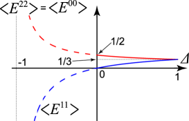
Figure 1: One-point functions of spin-1 XXZ chain in the massless regime obtained by the explicit evaluations of multiple integrals. The red and blue lines represent those for $\langle E^{22}\rangle=\langle E^{00}\rangle$ and $\langle E^{11}\rangle$, respectively.

Furthermore, we have confirmed the relations among the correlation functions due to the quantum group $U_{q}(sl_{2})$ symmetry and the spin inversion symmetry as follows

$$\langle\widetilde{E}^{1,1(2p)}\rangle=2\langle e_{1}^{0,0}e_{2}^{1,1}\rangle=2\langle e_{1}^{1,1}e_{2}^{0,0}\rangle=2\langle e_{1}^{0,1}e_{2}^{1,0}\rangle=2\langle e_{1}^{1,0}e_{2}^{0,1}\rangle.$$

In the XXX limit $\Delta\to 1$ we have $\langle E^{22}\rangle=\langle E^{11}\rangle=\langle E^{00}\rangle=1/3$, which has been shown by Kitanine in the XXX case [18]. In the free Fermion limit $\Delta\to 0$ we have $\langle E^{22}\rangle=\langle E^{00}\rangle=1/2$, and $\langle E^{11}\rangle=0$. Here we should remark that we consider the region $0\leq\zeta<\pi/(2s)$ with $s=1$, namely, $0<\Delta\leq 1$.

Finally, we confirm the analytical results by comparing them with the numerical results of exact diagonalization, which are shown in Fig. 2. In Fig. 2, the red and blue lines represent the analytical results obtained by evaluating the multiple integrals of the one-point functions, $\langle E^{22}\rangle=\langle E^{00}\rangle$ and $\langle E^{11}\rangle$, respectively. The black dotted lines represent the numerical estimates of the one-point functions which are obtained by the method of exact diagonalization of the integrable spin-1 XXZ Hamiltonian with the system size of $N_{s}=8$. We numerically obtain the ground-state eigenvector of the integrable spin-1 XXZ Hamiltonian, and calculate the numerical estimates of the one-point functions.

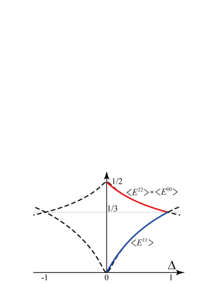
Figure 2: Comparison with the exact numerical diagonalization. The red and blue lines represent analytical results obtained by the multiple integrals for $\langle E^{22}\rangle=\langle E^{00}\rangle$ and $\langle E^{11}\rangle$, respectively. The black dotted lines represent those obtained by exact diagonalization with the system size $N_{s}=8$.

We have found that the numerical and analytical results of the spin-1 one-point functions agree quite well in the region $0<\Delta\leq 1$, as shown in Fig. 2. We thus conclude that the numerical results should support the validity of the multiple-integral representations for the spin-1 one-point functions.

Appendix A Derivation of reduction formula (2.10)

For the spin-$\ell/2$ Hermitian elementary matrices associated with homogeneous grading, $\widetilde{E}^{i,j(\ell,+)}$, we introduce coefficients ${\widetilde{g}}_{i,j}$ by

$$\widetilde{||\ell,i\rangle}\langle\ell,j||=\sum_{\{\varepsilon_{\alpha}^{\prime}\}_{\ell}}\sum_{\{\varepsilon_{\beta}\}_{\ell}}{\widetilde{g}}_{i,j}(\{\varepsilon_{\alpha}^{\prime}\},\{\varepsilon_{\beta}\})e_{1}^{\varepsilon_{1}^{\prime},\,\varepsilon_{1}}\cdots e_{\ell}^{\varepsilon_{\ell}^{\prime},\,\varepsilon_{\ell}}\,.$$

Then, we have

$${\widetilde{g}}_{i,j}(\{\varepsilon_{\alpha}^{\prime}\},\{\varepsilon_{\beta}\})=\left[\begin{matrix}\ell\\ i\end{matrix}\right]_{q}\left[\begin{matrix}\ell\\ j\end{matrix}\right]_{q}^{-1}\left(\begin{matrix}\ell\\ i\end{matrix}\right)_{q}q^{i(i-1)/2-j(j-1)/2}q^{-(a(1)+\cdots+a(i)-i)+(b(1)+\cdots+b(j)-j)}.$$

We derive the reduction formula for the Hermitian elementary operators $\widetilde{E}^{i,j(\ell,+)}$ as follows

$$\widetilde{E}^{i,j(\ell,+)}={\widetilde{P}}^{(\ell)}\widetilde{E}^{i,j(\ell,\,+)}=\left[\begin{matrix}\ell\\ i\end{matrix}\right]_{q}\left[\begin{matrix}\ell\\ j\end{matrix}\right]_{q}^{-1}\left(\begin{matrix}\ell\\ i\end{matrix}\right)q^{i(i-1)/2-j(j-1)/2}\widetilde{||\ell,i\rangle}$$ (A.1)

$${}\times\sum_{\{\varepsilon_{\beta}\}_{\ell}}\sum_{\{\varepsilon_{\alpha}^{\prime}\}_{\ell}}\left(\langle\ell,i||\sigma_{a(1)}^{-}\cdots\sigma_{a(i)}^{-}||\ell,0\rangle q^{-(a(1)+\cdots+a(i)-i)}\right)\langle\ell,0||\sigma_{b(1)}^{+}\cdots\sigma_{b(j)}^{+}q^{b(1)+\cdots+b(j)-i}.$$

Here $\{\varepsilon_{\beta}\}_{\ell}$ is given by a sequence of 0 or 1 such that the number of integers $\beta$ for $1\leq\beta\leq\ell$ satisfying $\varepsilon_{\beta}=1$ is given by $j$, and $\{\varepsilon_{\alpha}^{\prime}\}_{\ell}$ is given by a sequence of 0 or 1 such that the number of integers $\alpha$ satisfying $\varepsilon_{\alpha}^{\prime}=1$ is given by $i$.

We can show the following property:

Lemma A.1 ([55]).

Let ${\bm{\alpha}}^{-}$ be a set of distinct integers $\{a(1),\ldots,a(i)\}$ satisfying $1\leq a(1)<\cdots<a(i)\leq\ell$, we have the following:

$$\langle\ell,i||\sigma_{a(1)}^{-}\cdots\sigma_{a(i)}^{-}||\ell,0\rangle q^{-(a(1)+\cdots+a(i))+i}=\left[\begin{matrix}\ell\\ i\end{matrix}\right]^{-1}q^{-i(i-1)/2},$$

which is independent of the set ${\bm{\alpha}}^{-}=\{a(1),a(2),\ldots,a(i)\}$.

Applying Lemma A.1 we show that the inside of the parentheses (or the round brackets) of equation (A.1) is independent of $a(k)$s. Making use of the following:

$$\sum_{\{\varepsilon_{\alpha}^{\prime}\}_{\ell}}1=\left(\begin{matrix}\ell\\ i\end{matrix}\right),$$

where $\varepsilon_{\alpha}^{\prime}$ are such a sequence of 0 or 1 that the number of $\varepsilon_{\alpha}^{\prime}=1$ is given by $i$. We thus have

$$\widetilde{E}^{i,j(\ell,+)}=\left[\begin{matrix}\ell\\ i\end{matrix}\right]_{q}\left[\begin{matrix}\ell\\ j\end{matrix}\right]_{q}^{-1}\left(\begin{matrix}\ell\\ i\end{matrix}\right)^{-1}q^{i(i-1)/2-j(j-1)/2}\widetilde{||\ell,i\rangle}\langle\ell,i||$$

$$\phantom{\widetilde{E}^{i,j(\ell,+)}=}{}\times\left(\begin{matrix}\ell\\ i\end{matrix}\right)\sum_{\{\varepsilon_{\beta}\}_{\ell}}\sigma_{a(1)}^{-}\cdots\sigma_{a(i)}^{-}||\ell,0\rangle\langle\ell,0||\sigma_{b(1)}^{+}\cdots\sigma_{b(j)}^{+}q^{-(a(1)+\cdots+a(i)-i)}q^{b(1)+\cdots+b(j)-i}$$

$$\phantom{\widetilde{E}^{i,j(\ell,+)}}{}=\left[\begin{matrix}\ell\\ i\end{matrix}\right]_{q}\left[\begin{matrix}\ell\\ j\end{matrix}\right]_{q}^{-1}q^{i(i-1)/2-j(j-1)/2}\widetilde{||\ell,i\rangle}\langle\ell,i||e^{-(i-j)\xi_{1}}\sum_{\{\varepsilon_{\beta}\}_{\ell}}\chi_{1\cdots\ell}e_{1}^{\varepsilon_{1}^{\prime},\varepsilon_{1}}\cdots e_{\ell}^{\varepsilon_{\ell}^{\prime},\,\varepsilon_{\ell}}\,\chi_{1\cdots\ell}^{-1}.$$

Here we recall that $\{\varepsilon_{\beta}\}_{\ell}$ is a sequence such that the number of integers $\beta$ of $1\leq\beta\leq\ell$ satisfying $\varepsilon_{\beta}=1$ is given by $j$. The integers $a(k)$ ($1\leq k\leq i)$ and $b(k)$ ($1\leq k\leq j)$ satisfying $1\leq a(1)<\cdots<a(i)\leq\ell$ and $1\leq b(1)<\cdots<b(j)\leq\ell$, respectively, are related to the sequences $\{\varepsilon_{\alpha}^{\prime}\}_{\ell}$ and $\{\varepsilon_{\beta}\}_{\ell}$ by the following relation [55]:

$$e_{1}^{\varepsilon_{1}^{\prime},\varepsilon_{1}}\cdots e_{\ell}^{\varepsilon_{\ell}^{\prime},\varepsilon_{\ell}}=e_{a(1)}^{1,0}\cdots e_{a(i)}^{1,0}e^{0,0}_{1}\cdots e^{0,0}_{\ell}e_{b(1)}^{0,1}\cdots e_{b(j)}^{0,1}.$$

Appendix B Useful integral formulas

$$\int_{-\infty}^{\infty}\frac{{\rm d}x}{\cosh x}=\pi,$$ (B.1)

$$\int_{-\infty}^{\infty}\frac{\cosh 2ax}{\cosh^{2}x}{\rm d}x=\frac{2\pi a}{\sin\pi a},\qquad\text{for}\quad|a|<1.$$ (B.2)

Acknowledgments

The authors would like to thank F. Göhmann, C. Matsui and K. Motegi for helpful comments. They are grateful for useful comments to many participants of the workshop RAQIS’10, June, 2010, LAPTH, Annecy, France. This work is partially supported by Grant-in-Aid for Scientific Research (C) No. 20540365. J. Sato is supported by Grant-in-Aid for JSPS fellows.

References

• [1]
• [2] Korepin V.E., Bogoliubov N.M., Izergin A.G., Quantum inverse scattering method and correlation functions, Cambridge Monographs on Mathematical Physics, Cambridge University Press, Cambridge, 1993.
• [3] Jimbo M., Miwa T., Algebraic analysis of solvable lattice models, CBMS Regional Conference Series in Mathematics, Vol. 85, American Mathematical Society, Providence, RI, 1995.
• [4] Kitanine N., Maillet J.M., Slavnov N.A., Terras V., On the algebraic Bethe ansatz approach to the correlation functions of the XXZ spin-1/2 Heisenberg chain, hep-th/0505006.
• [5] Jimbo M., Miki K., Miwa T., Nakayashiki A., Correlation functions of the XXZ model for $\Delta<-1$, Phys. Lett. A 168 (1992), 256–263, hep-th/9205055.
• [6] Jimbo M., Miwa T., Quantum KZ equation with $|q|=1$ and correlation functions of the XXZ model in the gapless regime, J. Phys. A: Math. Gen. 29 (1996), 2923–2958, hep-th/9601135.
• [7] Miwa T., Takeyama Y., Determinant formula for the solutions of the quantum Knizhnik–Zamolodchikov equation with $|q|=1$, in Recent Developments in Quantum Affine Algebras and Related Topics (Raleigh, NC, 1998), Contemp. Math., Vol. 248, Amer. Math. Soc., Providence, RI, 1999, 377–393, math.QA/9812096.
• [8] Slavnov N.A., Calculation of scalar products of wave functions and form factors in the framework of the algebraic Bethe ansatz, Theoret. and Math. Phys. 79 (1989), 502–508.
• [9] Maillet J.M., Sanchez de Santos J., Drinfel’d twists and algebraic Bethe ansatz, in L.D. Faddeev’s Seminar on Mathematical Physics, Amer. Math. Soc. Transl. Ser. 2, Vol. 201, Amer. Math. Soc., Providence, RI, 2000, 137–178, q-alg/9612012.
• [10] Kitanine N., Maillet J.M., Terras V., Form factors of the XXZ Heisenberg spin-1/2 finite chain, Nuclear Phys. B 554 (1999), 647–678, math-ph/9807020.
• [11] Maillet J.M., Terras V., On the quantum inverse scattering problem, Nuclear Phys. B 575 (2000), 627–644, hep-th/9911030.
• [12] Kitanine N., Maillet J.M., Terras V., Correlation functions of the XXZ Heisenberg spin-1/2 chain in a magnetic field, Nuclear Phys. B 567 (2000), 554–582.
• [13] Göhmann F., Klümper A., Seel A., Integral representations for correlation functions of the XXZ chain at finite temperature, J. Phys. A: Math. Gen. 37 (2004), 7625–7651, hep-th/0405089.
• [14] Damerau J., Göhmann F., Hasenclever N.P., Klümper A., Density matrices for finite segments of Heisenberg chains of arbitrary length, J. Phys. A: Math. Theor. 40 (2007), 4439–4453, cond-mat/0701463.
• [15] Jimbo M., Miwa T., Smirnov F., Hidden Grassmann structure in the XXZ model III: introducing the Matsubara direction, J. Phys. A: Math. Theor. 42 (2009), 304018, 31 pages, arXiv:0811.0439.
• [16] Sakai K., Dynamical correlation functions of the XXZ model at finite temperature, J. Phys. A: Math. Theor. 40 (2007), 7523–7542, cond-mat/0703319.
• [17] Kitanine N., Kozlowski K.K., Maillet J.M., Slavnov N.A., Terras V., Algebraic Bethe ansatz approach to the asymptotic behavior of correlation functions, J. Stat. Mech. Theory Exp. 2009 (2009), P04003, 66 pages, arXiv:0808.0227.
• [18] Kitanine N., Correlation functions of the higher spin XXX chains, J. Phys. A: Math. Gen. 34 (2001), 8151–8169, math-ph/0104016.
• [19] Castro-Alvaredo O.A., Maillet J.M., Form factors of integrable Heisenberg (higher) spin chains, J. Phys. A: Math. Theor. 40 (2007), 7451–7471, hep-th/0702186.
• [20] Deguchi T., Matsui C., Form factors of integrable higher-spin XXZ chains and the affine quantum-group symmetry, Nuclear Phys. B 814 (2009), 405–438, arXiv:0807.1847.
• [21] Deguchi T., Matsui C., Correlation functions of the integrable higher-spin XXX and XXZ spin chains through the fusion method, Nuclear Phys. B 831 (2010), 359–407, arXiv:0907.0582.
• [22] Deguchi T., Matsui C., Algebraic aspects of the correlation functions of the integrable higher-spin XXX and XXZ spin chains with arbitrary entries, in the Proceedings of “Infinite analysis 09 – New Trends in Quantum Integrable Systems” (July 27–31, 2009, Kyoto University, Japan), to appear, arXiv:1005.0888.
• [23] Terras V., Drinfel’d twists and functional Bethe ansatz, Lett. Math. Phys. 48 (1999), 263–276, math-ph/9902009.
• [24] Bougourzi A.H., Weston R.A., $N$-point correlation functions of the spin-1 XXZ model, Nuclear Phys. B 417 (1994), 439–462, hep-th/9307124.
• [25] Göhmann F., Seel A., Suzuki J., Correlation functions of the integrable isotropic spin-1 chain at finite temperature, J. Stat. Mech. Theory Exp. 2010 (2010), P11011, 43 pages, arXiv:1008.4440.
• [26] Zamolodchikov A.B., Fateev V.A., A model factorized $S$-matrix and an integrable spin-1 Heisenberg chain, Soviet J. Nuclear Phys. 32 (1980), 298–303.
• [27] Kulish P.P., Reshetikhin N.Yu., Sklyanin E.K., Yang–Baxter equation and representation theory. I, Lett. Math. Phys. 5 (1981), 393–403.
• [28] Babujian H.M., Exact solution of the one-dimensional isotropic Heisenberg chain with arbitrary spins $s$, Phys. Lett. A 90 (1982), 479–482.
• [29] Babujian H.M., Exact solution of the isotropic Heisenberg chain with arbitrary spins: thermodynamics of the model, Nuclear Phys. B 215 (1983), 317–336.
• [30] Sogo K., Akutsu Y., Abe T., New factorized $S$-matrix and its application to exactly solvable $q$-state model. I, Progr. Theoret. Phys. 70 (1983), 730–738.
Sogo K., Akutsu Y., Abe T., New factorized $S$-matrix and its application to exactly solvable $q$-state model. II, Progr. Theoret. Phys. 70 (1983), 739–746.
• [31] Babujian H.M., Tsvelick A.M., Heisenberg magnet with an arbitrary spin and anisotropic chiral field, Nuclear Phys. B 265 (1986), 24–44.
• [32] Kirillov A.N., Reshetikhin N.Yu., Exact solution of the integrable XXZ Heisenberg model with arbitrary spin. I. The ground state and the excitation spectrum, J. Phys. A: Math. Gen. 20 (1987), 1565–1585.
• [33] Deguchi T., Wadati M., Akutsu Y., Exactly solvable models and new link polynomials. V. Yang–Baxter operator and braid-monoid algebra, J. Phys. Soc. Japan 57 (1988), 1905–1923.
• [34] Takhtajan L.A., The picture of low-lying excitations in the isotropic Heisenberg chain of arbitrary spins, Phys. Lett. A 87 (1982), 479–482.
• [35] Sogo K., Ground state and low-lying excitations in the Heisenberg XXZ chain of arbitrary spin $S$, Phys. Lett. A 104 (1984), 51–54.
• [36] Johannesson H., Central charge for the integrable higher-spin XXZ model, J. Phys. A: Math. Gen. 21 (1988), L611–L614.
• [37] Johannesson H., Universality classes of critical antiferromagnets, J. Phys. A: Math. Gen. 21 (1988), L1157–L1162.
• [38] Alcaraz F.C., Martins M.J., Conformal invariance and critical exponents of the Takhtajan–Babujian models, J. Phys. A: Math. Gen. 21 (1988), 4397–4413.
• [39] Affleck I., Gepner D., Schultz H.J., Ziman T., Critical behavior of spin-$s$ Heisenberg antiferromagnetic chains: analytic and numerical results, J. Phys. A: Math. Gen. 22 (1989), 511–529.
• [40] Dörfel B.-D., Finite-size corrections for spin-$S$ Heisenberg chains and conformal properties, J. Phys. A: Math. Gen. 22 (1989), L657–L662.
• [41] Avdeev L.V., The lowest excitations in the spin-$s$ XXX magnet and conformal invariance, J. Phys. A: Math. Gen. 23 (1990), L485–L492.
• [42] Alcaraz F.C., Martins M.J., Conformal invariance and the operator content of the XXZ model with arbitrary spin, J. Phys. A: Math. Gen. 22 (1989), 1829–1858.
• [43] Frahm H., Yu N.-C., Fowler M., The integrable XXZ Heisenberg model with arbitrary spin: construction of the Hamiltonian, the ground-state configuration and conformal properties, Nuclear Phys. B 336 (1990), 396–434.
• [44] Frahm H., Yu N.-C., Finite-size effects in the XXZ Heisenberg model with arbitrary spin, J. Phys. A: Math. Gen. 23 (1990), 2115–2132.
• [45] de Vega H.J., Woynarovich F., Solution of the Bethe ansatz equations with complex roots for finite size: the spin $S\geq 1$ isotropic and anisotropic chains, J. Phys. A: Math. Gen. 23 (1990), 1613–1626.
• [46] Klümper A., Batchelor M.T., An analytic treatment of finite-size corrections in the spin-1 antiferromagnetic XXZ chain, J. Phys. A: Math. Gen. 23 (1990) L189–L195.
• [47] Klümper A., Batchelor M.T., Pearce P.A., Central charge of the 6- and 19-vertex models with twisted boundary conditions, J. Phys. A: Math. Gen. 24 (1991), 3111–3133.
• [48] Suzuki J., Spinons in magnetic chains of arbitrary spins at finite temperatures, J. Phys. A: Math. Gen. 32 (1999), 2341–2359, cond-mat/9807076.
• [49] Idzumi M., Calculation of correlation functions of the spin-1 XXZ model by vertex operators, PhD Thesis, University of Tokyo, 1993.
• [50] Idzumi M., Correlation functions of the spin 1 analog of the XXZ model, hep-th/9307129.
• [51] Idzumi M., Level two irreducible representations of $U_{q}(\widehat{sl_{2}})$, vertex operators, and their correlations, Internat. J. Modern Phys. A 9 (1994), 4449–4484, hep-th/9310089.
• [52] Konno H., Free-field representation of the quantum affine algebra $U_{q}(\widehat{sl_{2}})$ and form factors in the higher-spin XXZ model, Nuclear Phys. B 432 (1994), 457–486, hep-th/9407122.
• [53] Kojima T., Konno H., Weston R., The vertex-face correspondence and correlation functions of the eight-vertex model. I. The general formalism, Nuclear Phys. B 720 (2005), 348–398, math.QA/0504433.
• [54] Deguchi T., Matsui C., On the evaluation of form factors and correlation functions for the integrable spin-$s$ XXZ chains via the fusion method, arXiv:1103.4206.
Deguchi T., Matsui C., Erratum to “Form factors of integrable higher-spin XXZ chains and the affine quantum-group symmetry” (Nuclear Phys. B 814 (2009), 405–438), Nuclear Phys. B, to appear.
• [55] Deguchi T., Reduction formula of form factors for the integrable spin-$s$ XXZ chains and application to the correlation functions, arXiv:1105.4722.
• [56] Boos H.E., Korepin V.E., Evaluation of integrals representing correlators in XXX Heisenberg spin chain, in MathPhys Odyssey 2001, Prog. Math. Phys., Vol. 23, Birkhäuser Boston, Boston, MA, 2002, 65–108, hep-th/0105144.
• [57] Takahashi M., Half-filled Hubbard model at low temperature, J. Phys. C: Solid State Phys. 10 (1977), 1289–1293.
• [58] Sakai K., Shiroishi M., Nishiyama Y., Takahashi M., Third-neighbor correlators of a one-dimensional spin-1/2 Heisenberg antiferromagnet, Phys. Rev. E 67 (2003), 065101, 4 pages, cond-mat/0302564.
• [59] Kato G., Shiroishi M., Takahashi M., Sakai K., Next nearest-neighbor correlation functions of the spin-1/2 XXZ chain at critical region, J. Phys. A: Math. Gen. 36 (2003), L337–L344, cond-mat/0304475.
• [60] Takahashi M., Kato G., Shiroishi M., Next nearest-neighbor correlation functions of the spin-1/2 XXZ chain at massive region, J. Phys. Soc. Japan 73 (2004), 245–253, cond-mat/0308589.
• [61] Kato G., Shiroishi M., Takahashi M., Sakai K., Third-neighbor and other four-point correlation functions of spin-1/2 XXZ chain, J. Phys. A: Math. Gen. 37 (2004), 5097–5123, cond-mat/0402625.
• [62] Boos H.E., Korepin V.E., Smirnov F.A., Emptiness formation probability and quantum Knizhnik–Zamolodchikov equation, Nuclear Phys. B 658 (2003), 417–439, hep-th/0209246.
• [63] Boos H.E., Shiroishi M., Takahashi M., First principle approach to correlation functions of spin-1/2 Heisenberg chain: fourth-neighbor correlators, Nuclear Phys. B 712 (2005), 573–599, hep-th/0410039.
• [64] Sato J., Shiroishi M., Fifth-neighbor spin-spin correlator for the anti-ferromagnetic Heisenberg chain, J. Phys. A: Math. Gen. 38 (2005), L405–L411, hep-th/0504008.
• [65] Sato J., Shiroishi M., Takahashi M., Correlation functions of the spin-1/2 anti-ferromagnetic Heisenberg chain: exact calculation via the generating function, Nuclear Phys. B 729 (2005), 441–466, hep-th/0507290.
• [66] Sato J., Shiroishi M., Takahashi M., Exact evaluation of density matrix elements for the Heisenberg chain, J. Stat. Mech. Theory Exp. 2006 (2006), P12017, 27 pages, hep-th/0611057.
• [67] Razumov A.V., Stroganov Yu.G., Spin chains and combinatorics, J. Phys. A: Math. Gen. 34 (2001), 3185–3190, cond-mat/0012141.
• [68] Kitanine N., Maillet J.M., Slavnov N.A., Terras V., Emptiness formation probability of the XXZ spin-1/2 Heisenberg chain at $\Delta=1/2$, J. Phys. A: Math. Gen. 35 (2002), L385–L391, hep-th/0201134.
• [69] Kitanine N., Maillet J.M., Slavnov N.A., Terras V., Exact results for the $\sigma^{z}$ two-point function of the XXZ chain at $\Delta=1/2$, J. Stat. Mech. Theory Exp. 2005 (2005), L09002, 7 pages, hep-th/0506114.
• [70] Sato J., Shiroishi M., Density matrix elements and entanglement entropy for the spin-1/2 XXZ chain at $\Delta=1/2$, J. Phys. A: Math. Theor. 40 (2007), 8739–8749, arXiv:0704.0850.
• [71] Jimbo M., A $q$-difference analogue of $U(g)$ and the Yang–Baxter equation, Lett. Math. Phys. 10 (1985), 63–69.
• [72] Jimbo M., A $q$-analogue of $U(gl(N+1))$, Hecke algebra and the Yang–Baxter equation, Lett. Math. Phys. 11 (1986), 247–252.
• [73] Drinfel’d V.G., Quantum groups, in Proceedings of the International Congress of Mathematicians, Vols. 1, 2 (Berkeley, Calif., 1986), Amer. Math. Soc., Providence, RI, 1987, 798–820.
• [74] Göhmann F., Korepin V.E., Solution of the quantum inverse problem, J. Phys. A: Math. Gen. 33 (2000), 1199–1220, hep-th/9910253.
\LastPageEnding