Cross section for double charmonium production in electron-positron annihilation at energy $\sqrt{s}$= 10.6 GeV

Abstract

In this work we study the process $e^{+}+e^{-}\longrightarrow J/\Psi+\eta_{c}$ at energy $\sqrt{s}=10.6GeV$ observed recently at B-factories whose measurements were made by Babar and Belle groups. We calculate the cross section for this process in the Bethe-salpeter formalism under Covariant Instantaneous Anstaz (CIA). To simplify our calculation, the heavy quark approximation is employed in the quark and gluon propagators. In the exclusive process of $e^{+}e^{-}$ annihilation into two heavy quarkonia, the cross section calculated in this scenario is compatible with the experimental data of Babar and Belle.

12.39.-x, 11.10.St , 21.30.Fe , 12.40.Yx , 13.20.-v

I Introduction

In this work we study the exclusive production process $e^{-}+e^{+}\rightarrow J/\psi+\eta_{c}$ at energy $\sqrt{s}=10.6GeV$ observed at B-factories [1,2,3] whose measurements have recently been done by Babar and Belle groups. It is well known that there was a significant discrepancy between the experimental measurements 1 ; 2 ; 3 and the non-relativistic QCD (NRQCD)4 ; 5 predictions for this process at centre of mass energies $\sqrt{s}\approx 10.6GeV$. This process has been recently studied in a Bethe-Salpeter formalism 6 in Instantaneous Approximation (IA). To simplify calculations, the authors have employed heavy quark limit in the propagators for studying systems composed of heavy charm and anti-charm quarks.

We wish to mention that Bethe-Salpeter equation (BSE) is a conventional non-perturbative approach in dealing with relativistic bound state problems in QCD. It is firmly established in the framework of field theory and from the solutions we can obtain useful information about the inner structure of hadrons, which is also crucial in treating high energy hadronic scattering and production processes. Despite its drawback of having to input model-dependent kernel, these studies have become an interesting topic in recent years, since calculations have shown that BSE framework using phenomenological potentials can give satisfactory results as more and more data is being accumulated. Further by adopting this framework we get more insight about the treatment of this process. This is mainly due to the unambiguous definition of BS wave function which is expressible by time ordered product of Heisenberg picture operators. This provides exact effective coupling vertex for bound state particle with all its N (N = 2 for mesons) constituents and can be considered as summing up all the non-perturbative QCD effects in the bound state.

On lines of 6 , we try to study this process in the framework of BSE under Covariant Instantaneous Ansatz (CIA) which is a Lorentz- invariant generalization of Instantaneous Approximation (IA). What distinguishes CIA from the other 3D reductions of BSE is its capacity for a two-way connection: an exact 3D BSE reduction for a $\mathrm{q}\overline{\mathrm{q}}$ system, and an equally exact reconstruction of original 4D BSE, the former to make contact with the mass spectrum, while the latter for calculation of transition amplitudes as 4D quark-loop integrals mitra01 ; a ; a1 ; bhatnagar06 ; bhatnagar09 . We wish to emphasise here that in these studies one of the main ingredients is the Dirac structure of the Bethe-Salpeter wave function (BSW). The copious Dirac structure of BSW was already studied by Llewllyn Smith smith69 much earlier. Recent studies cvetic04 ; alkofer02 have revealed that various covariant structures in BSWs of various hadrons are necessary to obtain quantitatively accurate observables. It has been further noticed that all covariants do not contribute equally for calculation of meson observables. To address this problem, recently we thought of investigating how to arrange these covariants systematically in BSWs. Thus, in a recent work bhatnagar06 , we developed a power counting rule for incorporating various Dirac structures in BSW, order-by-order in powers of inverse of meson mass. According to this power counting rule,the Leading order (LO) covariants are expected to contribute maximum to calculation of any meson observable, followed by the next-to-leading order (NLO) covariants. Taking in view of this fact, as a first step we have outlined the Dirac covariants and expanded the coefficients to the leading order (LO), and calculated the leptonic decay constants of vector mesons bhatnagar06 as well as pseudoscalar mesons bhatnagar09 at this order. The results were found to be close to data. In another recent work bhatnagar11 , we studied leptonic decay constants of unequal mass pseudoscalar mesons like $\pi,K,D,D_{s}$and $B$ and radiative decays of equal mass pseudoscalar mesons like $\pi^{0},\eta_{c}$ by taking into account both the leading order (LO) and Next-to-Leading Order (NLO) Dirac covariants. It was found that the contribution of leading order (LO) covariants to decay constants was maximum (about 90-95 percent) for heavier mesons composed of c and b quarks like $D$,$D_{s}$,$B$ and $\eta_{c}$ bhatnagar11 , while there was little contribution from NLO covariants. We now calculate the cross section for the process $e^{-}+e^{+}\rightarrow J/\psi+\eta_{c}$ by employing the most leading of the LO covariants (such as $\gamma_{5}$ for heavy pseudoscalar mesons like $\eta_{c}$ and $i\gamma.\varepsilon$ for heavy vector meson like $J/\psi$ comprising of heavy charm and anti-charm quarks for which BS formalism is quite suitable. In order to simplify the calculation, we will further impose the heavy quark approximation ($P\sim M,q<<M$) on the quark and gluon propagators to simplify the integrals as in Ref.6 . Under this approximation, our results are comparable with the data 1 ; 2 ; 3 . The remainder of this paper is organized as follows: In sec.II, we will study the BS equations for vector and pseudoscalar quarkonia. In sec.III, we will calculate the amplitude and cross section for the process $e^{+}+e^{-}\longrightarrow J/\Psi+\eta_{c}$ in the BS formalism. Sec.IV is reserved for conclusions and discussions.

II The Bethe-Salpeter Wave Function under CIA

We briefly outline the BSE framework under CIA. For simplicity, lets consider a $\mathrm{q}\overline{\mathrm{q}}$ system comprising of scalar quarks with an effective kernel $K$, 4D wave function $\Phi(P,q)$, and with the 4D BSE,

$$i(2\pi)^{4}\Delta_{1}\Delta_{2}\Phi(P,q)=\int d^{4}q^{\prime}K(q,q^{\prime})\Phi(P,q^{\prime}),$$ (1)

where $\Delta_{1,2}=m_{1,2}^{2}+p_{1,2}^{2}$are the inverse propagators, and $m_{1,2}$ are (effective) constituent masses of quarks. The 4-momenta of the quark and anti-quark, $p_{1,2}$, are related to the internal 4-momentum $q_{\mu}$ and total momentum $P_{\mu}$ of hadron of mass $M$ as $p_{1,2}{}_{\mu}=\widehat{m}_{1,2}P_{\mu}\pm q_{\mu},$ where $\widehat{m}_{1,2}=[1\pm(m_{1}^{2}-m_{2}^{2})/M^{2}]/2$ are the Wightman-Garding (WG) definitions of masses of individual quarks. Now it is convenient to express the internal momentum of the hadron $q$ as the sum of two parts, the transverse component, $\hat{q}_{\mu}=q_{\mu}-\frac{q.P}{P^{2}}P_{\mu}$ which is orthogonal to total hadron momentum $P$ (ie. $\widehat{q}.P=0$ regardless of whether the individual quarks are on-shell or off-shell), and the longitudinal component, $\sigma P_{\mu}=(q\cdot P/P^{2})P_{\mu}$, which is parallel to P. To obtain Hadron-quark vertex, use an Ansatz on the BS kernel $K$ in Eq. (1) which is assumed to depend on the 3D variables $\hat{q}_{\mu}$, $\hat{q}_{\mu}^{\prime}$ mitra01 ; a ; bhatnagar06 ; bhatnagar09 ; bhatnagar11 i.e.

$$K(q,q^{\prime})=K(\hat{q},\hat{q}^{\prime}),$$ (2)

(A similar form of the BS kernel was also earlier suggested in ref. resag94 ). Hence, the longitudinal component, $\sigma P_{\mu}$ of $q_{\mu}$, does not appear in the form $K(\hat{q},\hat{q}^{\prime})$ of the kernel. For reducing Eq.(1) to the 3D form of BSE, we define a 3D wave function $\phi(\widehat{q})$as,

$$\phi(\hat{q})=\int^{+\infty}_{-\infty}Md\sigma\Phi(P,q)$$ (3)

Substituting Eq.(3) in Eq.(1), with the definition of the kernel in Eq.(2), we get a covariant version of the Salpeter equation which is in fact a 3D BSE:

$$(2\pi)^{3}D(\hat{q})\phi(\hat{q})=\int d^{3}\hat{q}^{\prime}K(\hat{q},\hat{q}^{\prime})\phi(\hat{q}^{\prime}).$$ (4)

Here $D(\hat{q})$ is the 3D denominator function defined below whose value is obtained by evaluating contour integration over inverse quark propagators in the complex $\sigma$-plane by noting their corresponding pole positions bhatnagar05 ; bhatnagar06 ; bhatnagar09 as,

$$\frac{1}{D(\hat{q})}=\frac{1}{2\pi i}\int\limits_{-\infty}^{+\infty}\frac{Md\sigma}{\Delta_{1}\Delta_{2}}=\frac{\frac{1}{2\omega_{1}}+\frac{1}{2\omega_{2}}}{(\omega_{1}+\omega_{2})^{2}-M^{2}};\omega_{1,2}^{2}=m_{1,2}^{2}+\hat{q}^{2}.$$ (5)

We note that the RHS of Eq.(4) is exactly identical to the RHS of Eq.(1) by virtue of Eq.(2) and Eq.(3). We thus have an exact interconnection between 3D BSE and the 4D BSE, and hence between the 3D wave function$\phi(\hat{q})$ and the 4D wave function$\Phi(P,q)$mitra01 ; a ; a1 ; bhatnagar06 ; bhatnagar09 :

$$\Delta_{1}\Delta_{2}\Phi(P,q)=\frac{D(\hat{q})\phi(\hat{q})}{2\pi i}\equiv\Gamma(\hat{q}),$$ (6)

where $\Gamma(\hat{q})$ is the Bethe-Salpeter Hadron-quark vertex function for a meson comprising of scalar quarks.

The 4D BS wave function $\Phi(P,q)$ can be reconstructed from the 3D BS wave function $\phi(\hat{q})$ as:

$$\Phi(P,q)=\frac{1}{\Delta_{1}}\Gamma(\hat{q})\frac{1}{\Delta_{2}},$$ (7)

where $\Delta_{i}=(m_{i}^{2}+p_{i}^{2})$,(i=1,2) are the inverse propagators for scalar quarks which flank the hadron-quark vertex$\Gamma$. This 4D hadron-quark vertex $\Gamma(\hat{q})$ satisfies a 4D BSE with a natural off-shell extension over the entire 4D space (due to the positive definiteness of the quantity $\hat{q}^{2}=q^{2}-(q\cdot P)^{2}/P^{2}$ throughout the entire 4D space) and thus provides a fully Lorentz-invariant basis for evaluation of various transition amplitudes through various quark loop diagrams. Due to these properties, this framework of BSE under CIA can be profitably employed not only for low energy studies but also for evaluation of various transition amplitudes at quark level all the way from low energies to high energies. However this 4D hadron-quark vertex $\Gamma$ is still unnormalized and can be normalized as will be shown in the realistic case of fermionic quarks next.

For fermionic quarks the BSE under CIA can be written as:

$$i(2\pi)^{4}\Psi(P,q)=S_{F1}(p_{1})S_{F2}(p_{2})\int d^{4}q^{\prime}K(\widehat{q},\widehat{q}^{\prime})\Psi(P,q^{\prime}),$$ (8)

where the scalar propagators $\Delta_{i}^{-1}$ in the above equations are replaced by fermionic propagators $S_{F}$. Further the $H{q\bar{q}}$ vertex would be a $4\times 4$ matrix in the spinor space for which we should incorporate the relevant Dirac structures. For incorporation of the relevant Dirac structures in $\Gamma(\hat{q})$, they are incorporated order-by-order in powers of inverse of meson mass $M$, in accordance with the power counting rule we developed in bhatnagar06 . Our aim of developing the power counting rule was to find a “criterion” so as to systematically choose among various Dirac covariants from their complete set to write wave functions for different mesons (vector mesons, pseudoscalar mesons etc.)bhatnagar06 ; bhatnagar09 . In another recent work, we studied leptonic decay constants of unequal mass pseudoscalar mesons like $\pi,K,D,D_{s}andB$ and radiative decays of equal mass pseudoscalar mesons like $\pi^{0},\eta_{c}$ by taking into account both the leading order (LO) and Next-to-Leading Order (NLO) Dirac covariants. It was found that the contribution of leading order (LO) covariants to decay constants was maximum (about 90-95 percent) for heavier mesons composed of c and b quarks like $D$,$D_{s}$,$B$and $\eta_{c}$bhatnagar11 , while there was little contribution from NLO covariants. Among the LO covariants, it was also noticed that for pseudoscalar mesons, the contribution from covariant, $\gamma_{5}$was maximum and similarly for vector mesons, the contribution of LO covariant $i\gamma.\varepsilon$was maximum.

Thus to simplify the calculations, as a first step, we calculate the cross section for the process $e^{-}+e^{+}\rightarrow J/\psi+\eta_{c}$by employing the most leading of the LO covariants such as $\gamma_{5}$for heavy pseudoscalar mesons like $\eta_{c}$and $i\gamma.\varepsilon$for heavy vector meson like $J/\psi$comprising of heavy charm and anti-charm quarks for which BS formalism is quite suitable. The full fledged normalized 4D BS wave functions for a $q\bar{q}$ meson with quarks total momentum $P$and relative momentum $q$ and with individual quarks with momenta $p_{1}$ and $p_{2}$ can be written as:

$$\Psi(P,q)=S_{F}(p_{1})\Gamma(\hat{q})S_{F}(-p_{2})$$ (9)

where the 4D BS hadron-quark vertex function which absorbs the 4D BS normalizer N is,

$$\Gamma(\hat{q})=N\Gamma_{i}D(\hat{q})\phi(\hat{q})/2\pi i$$ (10)

where $\Gamma_{i}=\gamma_{5},i\gamma.\varepsilon,...$ are the relevant Dirac structures for pseudoscalar mesons, vector mesons etc. The 4D BS normalizer $N$ which is determined from standard current conserving conditions and is worked out in the framework of Covariant Instantaneous Ansatz (CIA) to give explicit covariance to the full fledged 4D BS wave function, $\Psi(P,q)$ and hence to the Hadron-quark vertex function, $\Gamma(\hat{q})$ employed for calculation of transition amplitudes at high energies.

Thus the 4D hadron-quark vertex function for $\eta_{c}$ is,

$$\Gamma^{P}(\widehat{q_{b}})=\gamma_{5}N_{P}D(\widehat{q_{b}})\phi(\widehat{q_{b}})/2\pi i,$$ (11)

while the 4D hadron-quark vertex function for $J/\Psi$ is,

$$\Gamma^{V}(\widehat{q_{a}})=i\gamma.\varepsilon N_{V}D(\widehat{q_{a}})\phi(\widehat{q_{a}})/2\pi i.$$ (12)

Here $N_{P}$ and $N_{V}$ are the 4D BS normalizers for $\eta_{c}$ and $J/\Psi$ meson (with internal momenta $q_{a}$ and $q_{b}$ respectively) which are determined through the current conservation condition mitra01 ; a ; bhatnagar06 ; bhatnagar09 ; bhatnagar11 , while $D(\widehat{q_{a}})$ and $D(\widehat{q_{b}})$ are the respective denominator functions. $\phi(\widehat{q_{a}})$ and $\phi(\widehat{q_{b}})$ are the 3D BS wave functions for $\eta_{c}$ and $J/\psi$ respectively, while $\varepsilon$ is the polarization vector for the $J/\psi$ meson.

As far as the input kernel $K(q,q^{\prime})$mitra01 ; a ; bhatnagar06 ; bhatnagar09 ; bhatnagar11 , in BSE is concerned, it is taken as one-gluon-exchange like as regards color [$(\bm{\lambda}^{(1)}/2)\cdot(\bm{\lambda}^{(2)}/2)$] and spin ($\gamma_{\mu}^{(1)}\gamma_{\mu}^{(2)}$) dependence. The scalar function $V(q-q^{\prime})$ is a sum of one-gluon exchange $V_{OGE}$ and a confining term $V_{conf}$. Thus we can write the interaction kernel as bhatnagar06 ; mitra01 :

$$K(q,q^{\prime})=\left(\frac{1}{2}\bm{\lambda}^{(1)}\right)\cdot\left(\frac{1}{2}\bm{\lambda}^{(2)}\right)V_{\mu}^{(1)}V_{\mu}^{(2)}V(q-q^{\prime});$$

$$V_{\mu}^{(1,2)}=\pm 2m_{1,2}\gamma_{\mu}^{(1,2)};$$

$$\begin{array}[]{rcl}V(\hat{q}-\hat{q}^{\prime})&=&\displaystyle\frac{4\pi\alpha_{S}(Q^{2})}{(\hat{q}-\hat{q}^{\prime})^{2}}+\frac{3}{4}\omega_{q\bar{q}}^{2}\int d^{3}\bm{r}\left[r^{2}(1+4a_{0}\hat{m}_{1}\hat{m}_{2}M^{2}r^{2})^{-1/2}-\frac{C_{0}}{\omega_{0}^{2}}\right]e^{i(\bm{\hat{q}-\hat{q}^{\prime}})\cdot\bm{r}};\\ &&\\ \alpha_{S}(Q^{2})&=&\displaystyle\frac{12\pi}{33-2f}\left(\ln\frac{Q^{2}}{\Lambda^{2}}\right)^{-1}.\end{array}$$ (13)

The Ansatz employed for the spring constant $\omega_{q\overline{q}}^{2}$ in Eq. (13) is mitra01 ; a ; bhatnagar06 ; bhatnagar09 ; bhatnagar11 ,

$$\omega_{q\overline{q}}^{2}=4\widehat{m}_{1}\widehat{m}_{2}M_{>}\omega_{0}^{2}\alpha_{S}(M_{>}^{2}),\quad M_{>}=Max(M,m_{1}+m_{2})$$ (14)

Here $\widehat{m}_{1}$, $\widehat{m}_{2}$ are the Wightman-Garding definitions of masses of constituent quarks defined earlier. Here the proportionality of $\omega_{q\bar{q}}^{2}$ on $\alpha_{S}(Q^{2})$ is needed to provide a more direct QCD motivation to confinement. This assumption further facilitates a flavour variation in $\omega_{q\bar{q}}^{2}$. And $\omega_{0}^{2}$ in Eq. (13) and Eq. (14) is postulated as a universal spring constant which is common to all flavours. Here in the expression for $V(\hat{q}-\hat{q}^{\prime})$, as far as the integrand of the confining term $V_{conf}$ is concerned, the constant term $C_{0}/\omega_{0}^{2}$ is designed to take account of the correct zero point energies, while $a_{0}$ term ($a_{0}\ll 1$) simulates an effect of an almost linear confinement for heavy quark sectors (large $m_{1}$, $m_{2}$), while retaining the harmonic form for light quark sectors (small $m_{1}$, $m_{2}$) mitra01 as is believed to be true for QCD. Hence the term $r^{2}(1+4a_{0}\widehat{m}_{1}\widehat{m}_{2}M_{>}^{2}r^{2})^{-1/2}$ in the above expression is responsible for effecting a smooth transition from harmonic ($q\overline{q}$) to linear ($Q\overline{Q}$) confinement . The values of basic constants are: $C_{0}=.29,\ \omega_{0}=0.158$ GeV, $m_{u,d}=0.265$ GeV, $m_{s}=0.415$ GeV, $m_{c}=1.530$ GeV and $m_{b}=4.900$ GeV which have been earlier fit to the mass spectrum of $q\overline{q}$ mesonsmitra01 obtained by solving the 3D BSE under Null-Plane Ansatz (NPA). However due to the fact that the 3D BSE under CIA has a structure which is formally equivalent to the 3D BSE under NPA, near the surface $P.q=0$, the $q\overline{q}$ mass spectral results in CIA formalism are exactly the same as the corresponding results under NPA formalismmitra01 ; a ; bhatnagar05 . The details of BS model under CIA in respect of spectroscopy are thus directly taken over from NPA formalism (For details, see mitra01 ; a ; bhatnagar05 ). As far as the 3D wave function $\phi(\hat{q})$ is concerned, it satisfies the 3D BSE on the surface P.q=0, which is appropriate for making contact with the mass spectra mitra01 . Its fuller structure is reducible to that of a 3D harmonic oscillator. The ground state wave function deducible from this equation has a gaussian structure and is expressible as $\phi(\hat{q})\approx e^{-\hat{q}^{2}/2\beta^{2}}$, where $\beta$ is the inverse range parameter which incorporates the content of BS dynamics and is dependent on the input kernel and is given as in mitra01 ; bhatnagar06 ; bhatnagar09 ). The structure of inverse range parameter $\beta$ in wave function $\phi(\widehat{q})$ is given asmitra01 ; bhatnagar06 ; bhatnagar09 :

$$\beta^{2}=(2\widehat{m}_{1}\widehat{m}_{2}M\omega_{q\bar{q}}^{2}/\gamma^{2})^{1/2};\gamma^{2}=1-\frac{2\omega_{q\bar{q}}^{2}C_{0}}{M_{>}\omega_{0}^{2}}$$ (15)

We now give the calculation of amplitude and cross section for the process $e^{-}+e^{+}\rightarrow J/\psi+\eta_{c}$ the leading order (LO) of QCD in the next section. We employ the hadron-quark vertex functions for $\eta_{c}$ and $J/\psi$ mesons given in Eq.(11) and (12) respectively in this calculation.

III Calculation of amplitude and cross section for the process $e^{+}+e^{-}\longrightarrow J/\Psi+\eta_{c}$

There are four Feynman diagrams in the leading order (LO) of QCD for the process $e^{+}+e^{-}\longrightarrow J/\Psi+\eta_{c}$. Two of these are depicted in Fig.1. The other two diagrams can be obtained by permutations. The details of momentum labeling of the diagram in Fig.1a is shown in Fig. 2 below. With reference to the momentum labeling in Fig.2, the adjoint BS wave function for $\eta_{c}$ meson can be written down as:

$$\overline{\Psi}(P_{b},q_{b})=S_{F}(-q_{2})\Gamma^{P}(\widehat{q_{b}})S_{F}(q_{4})$$ (16)

, while for $J/\psi$ meson, the adjoint BS wave function can be written as:

$$\overline{\Psi}(P_{a},q_{a})=S_{F}(-q_{3})\Gamma^{V}(\widehat{q_{a}})S_{F}(q_{1}^{\prime})$$ (17)

where $q_{a},q_{b}$ are the internal momenta of the hadrons $J/\Psi$ and $\eta_{c}$ respectively with the corresponding hadron-quark vertex functions $\Gamma^{V}$ and $\Gamma^{P}$ given in Eq.(11-12).

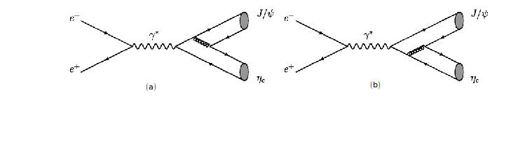
Figure 1: Two of the lowest order Feynman diagrams for the production of a pair of doubly heavy $c\overline{c}$ mesons in $e^{+}e^{-}$ annihilation. Other two diagrams can be obtained by permutations.

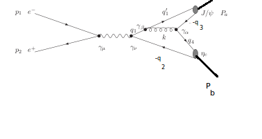
Figure 2: Momentum labeling of the first of the two Feynman diagrams shown in Fig.1

Using Feynman rules, one can obtain the amplitude for each of the diagrams in Fig.1. The amplitude corresponding to process in Fig.1a (described in detail in Fig.2) is given by

$$M_{1}=c\delta_{\mu\nu}ee_{Q}g_{s}^{2}\frac{1}{s}\overline{v}(p_{2})\gamma_{\mu}u(p_{1})\int d^{4}q_{a}d^{4}q_{b}Tr[\overline{\Psi}(P_{a},q_{a})\gamma_{\beta}S_{F}(q_{1})\gamma_{\nu}\overline{\Psi}(P_{b},q_{b})\gamma_{\alpha}]\frac{\delta_{\alpha\beta}}{k^{2}}$$ (18)

which can in turn be expressed as,

$$M_{1}= \frac{c\delta_{\mu\nu}ee_{Q}g_{s}^{2}}{s}\overline{v}(p_{2})\gamma_{\mu}u(p_{1})\int d^{4}q_{a}d^{4}q_{b}$$

$$\times Tr[S_{F}(-q_{3})\Gamma_{v}(\hat{q_{a}})S_{F}(q^{\prime}_{1})\gamma_{\beta}S_{F}(q_{1})\gamma_{\nu}S_{F}(-q_{2})\Gamma_{p}(\hat{q_{b}})S_{F}(q_{4})\gamma_{\alpha}]\frac{\delta_{\alpha\beta}}{k^{2}}$$

where c =$\frac{4}{3}$ is the color factor, the Mendelstam variable s is defined as, $s=-(p_{1}+p_{2})^{2}$ and $e_{Q}=2e/3$ is the electric charge of the charmed quark. The momentum relations of the quark and anti-quark in the final state are:

$$q_{1}^{\prime}=\frac{1}{2}P_{a}+q_{a},q_{3}=\frac{1}{2}P_{a}-q_{a},q_{4}=\frac{1}{2}P_{b}+q_{b},q_{2}=\frac{1}{2}P_{b}-q_{b},$$ (20)

and the momenta in the gluon and the quark propagators are given by

$$k=q_{3}+q_{4}=\frac{1}{2}(P_{a}+P_{b})-q_{a}+q_{b},$$ (21)

$$q_{1}=q_{1}^{\prime}+k=P_{a}+\frac{1}{2}P_{b}+q_{b},$$ (22)

respectively. As each of quark momenta in the quark propagators as well as the gluon propagator is going to depend upon the internal hadron momenta $q_{a}$ and $q_{b}$, the calculation of amplitude is going to involve integrations over these internal momenta and will be quite complex. Hence following 6 , we simplify the calculation, by employing the heavy quark approximation on the quark propagators, where we take the quark masses to be much larger than the internal momenta $q_{a}$ and $q_{b}$ of the hadrons. In this heavy quark approximation,we can use the approximation, $q_{a}<<M_{a},q_{b}<<M_{b}$. Thus we can write,

$$q_{a(b)}\ll P_{a(b)}\sim M_{a(b)},k=\frac{1}{2}(P_{a}+P_{b})-q_{a}+q_{b}\approx\frac{1}{2}(P_{a}+P_{b}),q_{1}=P_{a}+\frac{1}{2}P_{b}+q_{b}\approx P_{a}+\frac{1}{2}P_{b}.$$ (23)

With the above approximation, $k^{2}$ and $q_{1}^{2}$ are given by $k^{2}\approx-\frac{s}{4}$ and $q_{1}^{2}\approx-\frac{s}{2}-m_{c}^{2}.$ The propagators for the quarks and anti-quarks in momentum space in Eq.(16-17) are given by $S_{F}(q_{i})=\frac{-i}{i\gamma.q_{i}+m_{c}}$ =$\frac{-i(-i\gamma.q_{i}+m_{c})}{\Delta_{i}}$, where index $i$ labels the quark in the diagram.

Using Eq.(16) and (17) and the preceding expressions for the gluon and the quark propagators, the amplitude $M_{1}$ in Eq.(19) can be written as:

$$M_{1}=\frac{-2^{6}}{3^{2}s^{3}}g_{s}^{2}e^{2}\overline{v}(p_{2})\gamma_{\mu}u(p_{1})\int d^{4}q_{a}d^{4}q_{b}\frac{1}{\Delta_{2}\Delta_{3}\Delta_{4}\Delta_{5}}[TR]\frac{N_{v}D_{v}(\hat{q_{a}})\phi_{v}(\hat{q_{a}})}{2\pi i}\frac{N_{p}D_{p}(\hat{q_{b})}\phi_{p}(\hat{q_{b}})}{2\pi i}\\ .$$ (24)

Here [TR] is the trace over the gamma matrices appearing in the quark propagators in Eq.(19). Noting that the 4-dimensional volume element $d^{4}q=d^{3}\hat{q}Md\sigma$, we then perform contour integrations in the complex $\sigma$-plane by making use of the corresponding pole positions bhatnagar05 ; bhatnagar09 . The pole integrations over $dq_{a}^{0}=M_{a}d\sigma_{a}$ and $dq_{b}^{0}=M_{b}d\sigma_{b}$ in Eq.(24) can be expressed as:$\frac{1}{2\pi i}\int_{-\infty}^{\infty}\frac{M_{a}d\sigma_{a}}{\Delta_{3}\Delta_{5}}=\frac{1}{D(\hat{q_{a}})}$ and $\frac{1}{2\pi i}\int_{-\infty}^{\infty}\frac{M_{b}d\sigma_{b}}{\Delta_{2}\Delta_{4}}=\frac{1}{D(\hat{q_{b}})}$, where values of denominator functions $D(\hat{q}_{a})$ and $D(\hat{q}_{b})$ evaluated by contour integration in the complex $\sigma$- plane are expressible as in Eq.(5). After calculating the trace part in the above equation and employing the heavy quark approximation on relative momenta given in Eq.(23), one obtains:

$$M_{1}=\frac{-2^{14}\pi^{2}\alpha_{em}\alpha_{s}m_{c}^{3}}{3^{2}s^{3}}\epsilon_{\alpha\mu\lambda\sigma}\varepsilon_{\alpha}P_{b\lambda}P_{a\sigma}\int d^{3}\hat{q_{a}}d^{3}\hat{q_{b}}N_{v}N_{p}\phi_{v}(\hat{q_{a}})\phi_{p}(\hat{q_{b}})[\overline{v}(p_{2})\gamma_{\mu}u(p_{1})]$$ (25)

where $\alpha_{em}=\frac{e^{2}}{4\pi}$, while $\alpha_{s}=g_{s}^{2}/4\pi$ and is given in Eq.(13). Let’s define $\xi_{a}=\int d^{3}\hat{q_{a}}N_{v}\phi_{v}(\hat{q_{a}})$ and $\xi_{b}=\int d^{3}\hat{q_{b}}N_{p}\phi_{p}(\hat{q_{b}})$, which are values of wave functions at origins of $J/\psi$ and $\eta_{c}$ respectively.
Thus we can express the amplitude $M_{1}$ as,

$$M_{1}=\frac{-2^{14}\pi^{2}\alpha_{em}\alpha_{s}m_{c}^{3}}{3^{2}s^{3}}\epsilon_{\alpha\mu\lambda\sigma}\varepsilon_{\alpha}P_{b\lambda}P_{a\sigma}[\overline{v}(p_{2})\gamma_{\mu}u(p_{1})]\xi_{a}\xi_{b}$$ (26)

Here $N_{p}$ and $N_{v}$ in $\xi_{a,b}$ are the BS normalizers for $\eta_{c}$ and $J/\psi$ respectively which are evaluated by using the current conservation condition,

$$2iP_{\mu}=(2\pi)^{4}\int d^{4}qTr[\overline{\psi}(P,q)(\frac{\partial}{\partial P_{\mu}}S_{F}^{-1}(p_{1}))\psi(P,q)S_{F}^{-1}(-p_{2})]+(1\leftrightarrows 2)$$ (27)

Putting BS wave function $\psi(P,q)$ for a given meson in the above equation,carrying out derivatives of inverse quark propagators of constituent quarks with respect to total hadron momentum $P_{\mu}$, evaluating trace over gamma matrices, following usual steps and multiplying both sides of the equation by $P_{\mu}/(-M^{2})$ to extract out the normalizer N from the above equation, we then express the above expression in terms of integration variables $\hat{q}$ and $\sigma$. Noting that the 4-dimensional volume element $d^{4}q=d^{3}\hat{q}Md\sigma$, we then perform contour integration in the complex $\sigma$-plane by making use of the corresponding pole positions. For details of these mathematical steps involved in the calculation of BS normalizers for vector and pseudoscalar mesons, see Ref.bhatnagar06 and Ref.bhatnagar11 respectively, where in the present calculation we take only the leading order Dirac covariants $i\gamma.\varepsilon$ and $\gamma_{5}$ for $J/\psi$ and $\eta_{c}$ respectively in their respective 4D BS wave functions $\Psi(P,q)$. Then numerical integration on variable $\hat{q}$ is performed. The values of BS normalizers thus obtained for $J/\psi$ and $\eta$ mesons are $N_{v}=.0504GeV^{-3}$ and $N_{P}=.0410GeV^{-3}$ respectively.

The total amplitude for the process $e^{+}e^{-}\longrightarrow J/\Psi\eta_{c}$ can be obtained by summing over the amplitudes of all the four diagrams shown in Fig.1. For that matter the amplitude obtained from the first diagram is the same as the amplitude from each of the remaining three diagrams in Fig.1. Thus, the total amplitude is 4 times the amplitude from the first diagram. The unpolarized total cross section is obtained by summing over various $J/\Psi$ spin-states and averaging over those of the initial state $e^{+}e^{-}$. Thus, in the CM frame the total cross section, $\sigma$, is given by

$$\sigma=\frac{4m_{e}^{2}}{32\pi}\frac{\mid p_{f}\mid}{\mid p_{i}\mid(E_{1}+E_{2})^{2}}\int\frac{1}{4}\sum_{spin}\mid M_{tot}\mid^{2}dcos\theta$$ (28)

where $p_{f}$ is the momentum of either of the outgoing particles and $p_{i}$ is the momentum of either of the ingoing particles, which is in turn expressible as,

$$\sigma=\frac{4m_{e}^{2}}{32\pi}\frac{\sqrt{s-16m_{c}^{2}}}{s^{\frac{3}{2}}}\int\frac{1}{4}\sum_{spin}\mid M_{tot}\mid^{2}dcos\theta$$ (29)

where the masses of the leptons are ignored in the calculation. Explicitly $\mid M_{tot}\mid^{2}$ is given by

$$\frac{1}{4}\sum_{spin}\mid M_{tot}\mid^{2}=\frac{2^{30}\pi^{4}\alpha_{em}^{2}\alpha_{s}^{2}m_{c}^{6}}{3^{4}s^{5}4m_{e}^{2}}(-32m_{c}^{4}+t^{2}+u^{2})\xi_{a}^{2}\xi_{b}^{2}$$ (30)

where $t=-(p_{1}-P_{a})^{2}$ and $u=-(p_{1}-P_{b})^{2}$ are the Mandelstam’s variables. Therefore, in the CM frame, the total cross section is given by:

$$\sigma=\frac{2^{30}\pi^{3}\alpha_{em}^{2}\alpha_{s}^{2}m_{c}^{6}}{83^{5}s^{4}}(1-\frac{16m_{c}^{2}}{s})^{\frac{3}{2}}\xi_{a}^{2}\xi_{b}^{2}$$ (31)

Numerical Results:
The basic input parameters in the calculation are just four: $C_{0}=0.29$, $\omega_{0}=0.158GeV$, QCD length scale, $\Lambda_{QCD}=0.200GeV$, and the charmed quark mass, $m_{c}=1.530GeV$ bhatnagar06 ; bhatnagar09 . The numerical values of inverse range parameter $\beta$ calculated from Eq.(15) are $\beta_{J/\psi}=.4989GeV$ and $\beta_{\eta_{c}}=.4388GeV$. To calculate the values of $\beta$, for the two hadrons, the experimental hadron masses are taken as, $M_{J/\psi}=3.096GeV$ and $M_{\eta_{c}}=2.982GeV$. With these parameters the total cross section for the above process at $\sqrt{s}=10.6GeV$ is calculated to be $\sigma=21.75fb$.

IV Discussion

In this paper we have calculated the cross section of the exclusive process of $e^{+}e^{-}\longrightarrow J/\Psi\eta_{c}$ at energy $\sqrt{s}=10.6GeV$ in the framework of BSE under CIA bhatnagar09 ; bhatnagar11 ; bl07 using only the leading order (LO) diagrams in QCD. We find the theoretical value of $\sigma[e^{+}e^{-}\longrightarrow J/\Psi\eta_{c}]=21.75fb$, which is broadly in agreement with the Babar’s data $\sigma[e^{+}e^{-}\longrightarrow J/\Psi\eta_{c}]=(17.6\pm 2.8\pm 2.1)fb$ 1 and the Belle’s data, $\sigma[e^{+}e^{-}\longrightarrow J/\Psi\eta_{c}]=(25.6\pm 2.8\pm 3.4)fb$ 2 ; 3 .

It had been noticed earlier that NRQCD predictions 4 ; 5 for the above process at $\sqrt{s}=10.6GeV$ using leading order diagrams alone give cross sections which are much less than data 1 ; 2 ; 3 . Such a large discrepancy between experimental results and theoretical predictions has been a challenge to the understanding of charmonium production through NRQCD. Many studies were performed to resolve this problem. For instance Braaten and Leebraaten03 first showed that results on cross section are found to improve considerably when relativistic corrections are incorporated. Then it was found that to obtain cross sections from NRQCD which are consistent with data, one has to incorporate NLO QCD corrections gong07 ; zhang06 . However in these studies it was found that the value of total NLO contribution to cross section is nearly twice the LO contribution. In the present calculations under the relativistic framework of BSE under CIA, we obtained results for cross sections which are in good agreement with data1 ; 2 ; 3 using leading order QCD processes alone though we have employed the heavy quark approximation ($q<<M$ and $P\sim M$) on the quark and gluon propagators on lines of 6 . However we have not made use of the non-covariant heavy quark limit as in Eq.(3-4) of Ref.[6]and work with the exact propagators of the quarks constituting the two hadrons. This is a validation of the fact that BSE which is firmly rooted in field theory and which incorporates relativistic effects within its premises is ideally suited to describe not only low energy processes, but even processes at high energies such as high energy hadronic scatterings and production processes.

The approach in this paper is quite different from the approach in Ref.[6] is the sense that we employ the framework of BSE under CIA which is a relativistic generalization of Instantaneous Approximation (IA) used in the former and has a much wider range of applicability as explained in Section II of this paper. Further, to calculate their results, Ref.[6] has made use of heavy quark limit on the propagators of all the heavy quarks and anti-quarks, where the propagators have been simplified as in their Eq.(3) and (4) which in fact is non-relativistic and non-covariant. Also to simplify their calculation of amplitude in their Eq.(22), [6] makes use of the heavy quark approximation, in that the propagators of quark and gluon are independent of relative momenta $q_{a}$ and $q_{b}$ of the two hadrons since the masses of quarks are large compared to their relative momentum. However in our paper, we only make use of the above heavy quark approximation ($q<<M$ and $P\sim M$) only in the sense of simplifying the integrals involved in Eq.(18)-(19) for amplitude calculation as done in [6], but we do not employ the non-relativistic and non-covariant heavy quark limit on the quark and anti quark propagators (as in Eq.(3) and (4) of [6]) and instead work with the full quark and anti-quark propagators for the quarks constituting the hadrons. In doing so using CIA, we also see that our results on $\sum_{s}|M_{tot}|^{2}$ in Eq.(30) and cross section in Eq.(31) of our paper are not exactly similar to results of [6]. In this regard, we wish to point out that our amplitude and cross sectional formulae involve the 4D BS normalizers $N_{V}$ and $N_{P}$ which are calculated in the framework of CIA and whose numerical values are explicitly worked out for both the hadrons, $J/\psi$ and $\eta_{c}$ as $N_{v}=.0504GeV^{-3}$ and $N_{P}=.0410GeV^{-3}$ respectively. These normalizers enter the amplitude and cross sectional formulae through the definitions of values of wave functions$\xi_{a}$ and $\xi_{b}$ of the two hadrons at their origins, which is not so in case of Ref.[6]. Further, the input BSE kernel and hence the input parameters employed by us and by Ref.[6] are completely different. While we employ ”vector” confinement, ie. we make use of a common form $(\gamma_{\mu}^{(1)}\gamma_{\mu}^{(2)})$ for both one-gluon exchange as well as confining terms in the kernel as in Eq.(13) (seemitra01 ; bhatnagar06 for details) , Ref.[6] employs a scalar $(1^{(1)}.1^{(1)})$ form for confinement, while vector form $(\gamma_{\mu}^{(1)}\gamma_{\mu}^{(2)})$ for one-gluon exchange. Further the functional form of confining potential in [6]is also different from our case. Whereas Ref.[6] uses linear confinement $(\thicksim r)$ which is true in case of heavy quark (c,b) systems, we have used a general form of confinement potential in Eq.(13) which simulates the effect of linear confinement $(\thicksim r)$ for heavy quark sector (large $m_{1},m_{2})$ while retaining harmonic form $(\thicksim r^{2})$ for light quark sector (small $m_{1},m_{2})$ as explained in section 2. As far as the numerical results on cross section in this paper and Ref.[6] are concerned, they are quits close. This may be due to the fact that for systems comprising of heavy quarks (c,b), the CIA results may lead to IA results when heavy quark approximation is imposed. However this may not be so for systems comprising of light quarks (u,d,s).

However in the present calculation, we used only the first of the leading order(LO) Dirac covariants ($\gamma_{5}$ and $i\gamma.\varepsilon$)in hadron-vertex functions for $J/\psi$ and $\eta_{c}$ mesons respectively. They were identified as most leading covariants in accordance with our power counting scheme. These covariants give maximum contribution to calculation of meson observables such as decay constants etc. It can also be seen here that the results on cross section for the process $e^{+}e^{-}\longrightarrow J/\Psi+\eta_{c}$ employing these most leading of the LO covariants brings theoretical results close to data 1 ; 2 ; 3 . We now also intend to see the effect of incorporation of both LO and the NLO Dirac covariants (to the vertex functions of these mesons) on cross section for the process studied. The contribution from NLO covariants is expected to be much lesser than the contribution from LO covariants in line with our recent studies on meson decaysbhatnagar06 ; bhatnagar09 ; bhatnagar11 . And this is more so for heavy mesons comprising of c and b quarks. It is expected that the results of cross section will improve further with incorporation of both LO and NLO covariants and without employing the heavy quark approximation on the quark and gluon propagators. This calculation will be quite rigorous and will be the subject of a later communication.

Acknowledgements: This work was carried out in the Department of Physics, Addis Ababa University (AAU). The authors would like to thank the Physics Department,AAU for the facilities provided during the course of this work. One of us, EM would like to thank Haramaya University (HU) for supporting his doctoral programme.

REFERENCES:

REFERENCES:

- (1) B.Aubert et al.[BABAR Collaboration], Phys. Rev. D 72, 031101 (2005)[arxiv:hep-ex/0506062].
- (2) K.Abe et al., et al.[BELLE Collaboration], Phys. Rev. Lett. 89, 142001 (2002)[arxiv:hep-ex/0205104].
- (3) K.Abe et al., et al.[BELLE Collaboration], Phys. Rev. D 70, 071102 (2004)[arxiv:hep-ex/0407009].
- (4) G.Bodwin,E.Braaten,G. Lepage, Phys. Rev. D 51, 1125 (1995); 55, 5855(E) (1997).
- (5) K.Liu, Z.He, K.Chao, Phys. Lett. B 557, 45 (2003).
- (6) X-H Guo, H-W Ke, X-Q Li, X-H Wu, arxiv:0804.0949[hep-ph].
- (7) A. N. Mitra, B. M. Sodermark, Nucl. Phys. A 695, 328 (2001) and references therein.
- (8) S. Bhatnagar, D. S. Kulshreshtha, A. N. Mitra, Phys. Lett. B 263, 485 (1991).
- (9) A. N. Mitra, S. Bhatnagar, Intl. J. Mod. Phys. A 7, 121 (1992).
- (10) S. Bhatnagar, S-Y. Li, J. Phys. G 32, 949 (2006).
- (11) S.Bhatnagar, S-Y. Li, Intl. J. Mod. Phys. E 18, 1521(2009).
- (12) C. H. L. Smith, Ann. Phys. 53, 521 (1969).
- (13) G. Cvetic et al., Phys. Lett. B 596, 84 (2004).
- (14) R. Alkofer, P. Watson, H. Weigel, Phys. Rev. D 65, 094026 (2002).
- (15) S. Bhatnagar, S-Y.Li, J.Mahecha, Intl. J. Mod. Phys. E 20,1437 (2011).
- (16) J. Resag, C. R. Muenz, B. C. Metsch, H. R. Petry, Nucl. Phys. A 578, 397 (1994).
- (17) S. Bhatnagar, Intl. J. Mod. Phys. E 14, 909 (2005).
- (18) S. Bhatnagar and S. Y. Li, In the Proceedings of 9th Workshop on Non-Perturbative Quantum Chromodynamics, Paris, France, 4-8 Jun 2007, pp 12.
- (19) E.Braaten, J.Lee, Phys.Rev. D67, 054007 (2003).
- (20) B.Gong, J-X. Wang, Phys. Rev. D77, 054028 (2008).
- (21) Y.J.Zhang, Y.J.Gao, K.T.Chao, Phys. Rev. Lett. 96, 092001 (2006).