1) Department of Physics, IIT Kanpur, Kanpur 208 016, India
2) Institute of Physics, Bhubaneswar 751 005, India
3) Indian Institute of Science Education and Research, Bhopal 462 023, India

1   Introduction

Scale invariance is an idea with quite a long history. The possibility of local scale invariance was first suggested by Weyl [1] in the twenties. This subsequently lead to considerable research effort by several physicists [2, 3, 4, 5, 6, 7, 8, 9, 10, 11, 12, 13, 14, 15, 16, 17, 18, 19, 20]. Quantizing a scale invariant theory is considered problematic since scale invariance is anomalous in general. However, it has also been argued that in some cases it might be possible to preserve scale invariance in the full quantum field theory [21, 18, 22, 23]. Despite the difficulties scale invariance remains an interesting idea since it has the potential to resolve one of the greatest puzzle of physics, namely, the cosmological constant problem[18, 26, 23, 24, 25].

A scale invariant theory contains no dimensionful parameter in the action. Hence in any realistic theory scale invariance has to be broken in order to agree with observations. There exist several mechanisms to break scale invariance [27, 28, 29, 30, 31, 18, 32]. One such mechanism for breaking scale invariance is to assume the existence of a classical background cosmological solution [28, 18, 31, 32]. This may be demonstrated by including just one scalar field besides gravity. Consider the following action,

$$S=\int d^{4}x\sqrt{-g}\left[\frac{\beta\chi^{2}}{8}R+\frac{1}{2}D^{\mu}\chi D_{\mu}\chi-\frac{1}{4}\lambda\chi^{4}\right],$$ (1)

where $\chi$ is a real scalar field. This action is invariant under a global scale transformation,

$$\chi\rightarrow\chi\Lambda,\quad x\rightarrow x/\Lambda.$$ (2)

Here we have chosen the conventions followed in Refs. [33, 34] where the flat space-time metric takes the form $(1,-1,-1,-1)$ and the curvature tensor and its contractions are defined as,

$$R^{\mu}_{\nu\alpha\beta} = -\partial_{\beta}\Gamma^{\mu}_{\nu\alpha}+\partial_{\alpha}\Gamma^{\mu}_{\nu\beta}+\Gamma^{\mu}_{\gamma\alpha}\Gamma^{\gamma}_{\nu\beta}-\Gamma^{\mu}_{\gamma\beta}\Gamma^{\gamma}_{\nu\alpha},$$

$$R_{\nu\beta} = R^{\mu}_{\nu\beta\mu}\hskip 2.84526pt,\hskip 11.38109ptR=R_{\nu\beta}g^{\nu\beta}.$$ (3)

Now, we seek a constant solution of the equation of motion for the scalar field $\chi$, so that the term $\left(\beta\chi^{2}/8\right)$ in the action generates the effective gravitational constant. Hence we may drop the terms containing the derivatives of the scalar field in its equation of motion to obtain the following relation,

$${\beta R\over 4} = \lambda\chi^{2}\,.$$ (4)

Here $R$ represents the classical scale covariant curvature scalar, as defined in Eq. 3. We assume the FRW metric with the spatial curvature parameter $k=0$ and scale parameter $a(t)$ where $t$ is the cosmic time. We obtain a solution to the classical equations,

$$\chi=\chi_{0}={M_{\rm PL}\over\sqrt{2\pi\beta}}\,,$$ (5)

where $M_{\rm PL}$ is the Planck mass. The FRW scale parameter is given by

$$a(t)=a_{0}e^{H_{0}t},$$ (6)

where $H_{0}$ is the Hubble parameter. This sets the curvature scalar as $R=12H_{0}^{2}$. Hence we obtain the solution corresponding to the de Sitter space-time. The background field $\chi_{0}$, the Hubble constant $H_{0}$ and the curvature scalar $R$ are constant for this solution. One may of course obtain more realistic solutions by adding contributions from dark matter candidates as well as standard model particles [19]. One may also allow the scalar field $\chi$ to be time dependent [32]. In such cases $R$ will no longer be independent of time. This will complicate our analysis but will not be conceptually different from the simple case we consider. Hence in this paper we consider this simple case only.

The solution generates both the gravitational constant and an effective cosmological constant. It is interesting that an effective cosmological constant is generated, despite the fact that scale invariance forbids this term in the action. This might be indicative of the fundamental nature of this parameter [35]. We have argued in earlier papers that this mechanism for breaking scale invariance is different from spontaneous symmetry breaking. In the latter case one is interested in the behavior of the ground state of the Hamiltonian of matter fields under the symmetry transformation. Hence one makes a quantum expansion around the minimum of the potential. In the present case we seek a time dependent solution and the minimum of the potential is not directly relevant. The time dependence of the solution comes from the scale parameter, $a(t)$. In earlier papers we have called this phenomenon cosmological symmetry breaking [31, 18] in order to emphasize its difference from spontaneous symmetry breaking. The important question now is whether such a solution is stable or not. In this paper we investigate this question. We demonstrate the stability of this solution under small perturbations and hence show that it can consistently break scale invariance.

Such de Sitter or approximately de Sitter solutions have also been discussed in the case of general scalar-tensor theories. Several papers have addressed the issue of stability of these solutions [36, 37, 38] as well as computed the power spectrum of perturbations [39, 40, 41, 42, 43, 44, 45]. The power spectrum is useful if one assumes that this solution is applicable to inflation. The theory we consider is obtained as a special case of these scalar-tensor theories by imposing the constraint that the action must be invariant under scale transformations. The background de Sitter solution plays a crucial role in our case since it provides a mechanism to break scale symmetry. Indeed it is difficult to find alternate methods to break this symmetry. For example, this symmetry can be broken spontaneously only if we arbitrarily set some terms to zero in the action [22]. Since no symmetry prohibits such terms, these have to tuned to zero at each order in perturbation theory. In contrast our mechanism does not require any such constraint. Due to the special role played by the de Sitter solution in our model, testing the stability of this solution is crucial in our case. If the solution is found to be stable then it establishes the cosmological symmetry breaking as a robust mechanism to break scale and possibly other symmetries.

We may also directly use the results of stability analysis of the de Sitter solutions in general scalar-tensor theories and apply these to our special case. A general criteria for testing stability is given, for example, in Ref. [36, 37]. We find that our results are consistent with this condition, as discussed in Section 2.

The background de Sitter solution in our scale invariant model may be applicable to inflation or to dark energy. However in the present paper we are not interested in cosmological applications of this model and only in demonstrating that the solution is stable.

In the rest of this paper we shall use the conformal time $\eta$ instead of $t$. Hence the spatially flat FRW metric becomes,

$$g_{\mu\nu}=a^{2}(\eta)(1,-1,-1,-1)\,.$$ (7)

In terms of $\eta$ the Einstein’s equations, at the leading order, may be written as,

$$\left(\frac{a^{\prime}}{a}\right)^{2} = \frac{\lambda\chi_{0}^{2}a^{2}}{3\beta}\ ,$$

$$\left(\frac{a^{\prime\prime}}{a}\right) = 2\left(\frac{\lambda\chi_{0}^{2}a^{2}}{3\beta}\right)\ .$$ (8)

Here the primes represent derivatives with respect to $\eta$.

2   Perturbations

In this section we study the perturbations to the leading order solution. As already mentioned we shall restrict ourselves to small perturbations. The perturbed metric may be expressed as,

$$g_{\mu\nu}=a^{2}\left(\begin{array}[]{cc}1+2A&\partial_{i}B+M_{i}\\ \partial_{i}B+M_{i}&\left(-1+2\psi\right)\delta_{ij}-D_{ij}E+\partial_{j}V_{i}+\partial_{i}V_{j}+P_{ij}\end{array}\right)\ ,$$ (11)

where $a=a(\eta)$ is the scale factor of the universe in terms of the conformal time, $D_{ij}=\left(\partial_{i}\partial_{j}-\frac{1}{3}\delta_{ij}\nabla^{2}\right)$, $A,B,E$ and $\psi$ are the scalar perturbations, $V_{i}$ and $M_{i}$ are the vector perturbations and $P_{ij}$ stands for the pure tensor perturbations. The pure vector and the tensor parts satisfy the following constraints [46],

$$\partial_{i}V_{i}=\partial_{i}M_{i}=0;\ \ \partial_{i}P_{ij}=0;\ \ P_{ii}=0.$$ (12)

The inverse metric becomes,

$$g^{\mu\nu}=\frac{1}{a^{2}}\left(\begin{array}[]{cc}1-2A&\partial_{i}B+M_{i}\\ \partial_{i}B+M_{i}&\left(-1-2\psi\right)\delta_{ij}+D_{ij}E-\partial_{j}V_{i}-\partial_{i}V_{j}-P_{ij}\end{array}\right),$$ (15)

where we have neglected all the terms beyond the first order in perturbations. We also expand the field $\chi$ such that

$$\chi=\chi_{0}+\hat{\chi},$$ (16)

where $\chi_{0}$ represents the solution at leading order and $\hat{\chi}$ a small perturbation.

We express the Einstein equation as,

$$G_{\mu\nu} = T_{\mu\nu}\ ,$$ (17)

where,

$$G_{\mu\nu} = R_{\mu\nu}-\frac{1}{2}g_{\mu\nu}R,$$ (18)

$$T_{\mu\nu} = -\frac{\chi^{2}_{;\lambda;\kappa}}{\chi^{2}}\left(g^{\lambda}_{\mu}g^{\kappa}_{\nu}-g_{\mu\nu}g^{\lambda\kappa}\right)+\frac{4}{\beta\chi^{2}}\left(\frac{1}{2}g^{\rho\sigma}(\partial_{\rho}\chi)(\partial_{\sigma}\chi)-\frac{1}{4}\lambda\chi^{4}\right)g_{\mu\nu}$$ (19)

$$- \frac{4}{\beta\chi^{2}}(\partial_{\mu}\chi)(\partial_{\nu}\chi)\ .$$

Using the decomposition theorem [47, 48, 45], we can now decompose the Einstein’s equation into scalar, vector and tensor modes and treat their perturbations separately as these modes evolve independently [49, 50, 51]. The tensor modes are gauge invariant [52] and so gauge fixing is not required. However both in the case of the scalar and the vector modes we need to fix a gauge to get a physical solution.

2.1   Scalar modes:

For the scalar modes we choose the longitudinal (conformal Newtonian) gauge [53, 54, 55], $B=E=0$. At the first order in the perturbations, the components of the Einstein tensor are given by,

$$\delta G_{00} = -2\nabla^{2}\psi+6\frac{a^{\prime}}{a}\psi^{\prime}\ ,$$ (20)

$$\delta G_{0i} = -2\frac{a^{\prime}}{a}\partial_{i}A-2\partial_{i}\psi^{\prime}\ ,$$ (21)

$$\delta G_{ij} = \left(-\nabla^{2}\left(A-\psi\right)-2\frac{a^{\prime}}{a}A^{\prime}-4\frac{a^{\prime}}{a}\psi^{\prime}-2\psi^{\prime\prime}-\frac{2\lambda\chi_{0}^{2}a^{2}}{\beta}\left(A+\psi\right)\right)\delta_{ij}$$ (22)

$$+\partial_{i}\partial_{j}(A-\psi)\ .$$

The corresponding components of the energy momentum tensor are

$$\delta T_{00} = -2\nabla^{2}\left(\frac{\hat{\chi}}{\chi_{0}}\right)+6\left(\frac{a^{\prime}}{a}\right)\left(\frac{\hat{\chi}^{\prime}}{\chi_{0}}\right)-\frac{2\lambda\chi_{0}^{2}a^{2}}{\beta}\left(A+\left(\frac{\hat{\chi}}{\chi_{0}}\right)\right)\ ,$$ (23)

$$\delta T_{0i} = 2\left(\frac{a^{\prime}}{a}\right)\partial_{i}\left(\frac{\hat{\chi}}{\chi_{0}}\right)-2\partial_{i}\left(\frac{\hat{\chi^{\prime}}}{\chi_{0}}\right)\ ,$$ (24)

$$\delta T_{ij} = \left[2\nabla^{2}\left(\frac{\hat{\chi}}{\chi_{0}}\right)-2\left(\frac{a^{\prime}}{a}\right)\left(\frac{\hat{\chi}^{\prime}}{\chi_{0}}\right)-2\left(\frac{\hat{\chi}^{\prime\prime}}{\chi_{0}}\right)+\frac{2\lambda\chi_{0}^{2}a^{2}}{\beta}\left(\frac{\hat{\chi}}{\chi_{0}}-\psi\right)\right]\delta_{ij}$$ (25)

$$-2\partial_{i}\partial_{j}\left(\frac{\hat{\chi}}{\chi_{0}}\right).$$

Comparing all the components of the Einstein tensor and the energy momentum tensor we get,

$$-\nabla^{2}\psi+3\frac{a^{\prime}}{a}\psi^{\prime} = -\nabla^{2}\left(\frac{\hat{\chi}}{\chi_{0}}\right)+3\left(\frac{a^{\prime}}{a}\right)\left(\frac{\hat{\chi}^{\prime}}{\chi_{0}}\right)$$ (26)

$$-\frac{\lambda\chi_{0}^{2}a^{2}}{\beta}\left(A+\left(\frac{\hat{\chi}}{\chi_{0}}\right)\right),$$

$$-\frac{a^{\prime}}{a}\partial_{i}A-\partial_{i}\psi^{\prime} = \left(\frac{a^{\prime}}{a}\right)\partial_{i}\left(\frac{\hat{\chi}}{\chi_{0}}\right)-\partial_{i}\left(\frac{\hat{\chi^{\prime}}}{\chi_{0}}\right),$$ (27)

$$-\nabla^{2}\left(A-\psi\right)-3\frac{a^{\prime}}{a}A^{\prime}-6\frac{a^{\prime}}{a}\psi^{\prime}-3\psi^{\prime\prime} = 2\nabla^{2}\left(\frac{\hat{\chi}}{\chi_{0}}\right)-3\Big{[}\left(\frac{a^{\prime}}{a}\right)\left(\frac{\hat{\chi}^{\prime}}{\chi_{0}}\right)+\left(\frac{\hat{\chi}^{\prime\prime}}{\chi_{0}}\right)$$ (28)

$$-\frac{\lambda\chi_{0}^{2}a^{2}}{\beta}\left(\frac{\hat{\chi}}{\chi_{0}}-\psi\right)+\frac{\lambda\chi_{0}^{2}a^{2}}{\beta}\left(A+\psi\right)\Big{]}\ ,$$

$$\partial_{i}\partial_{j}\left(A-\psi\right) = -2\partial_{i}\partial_{j}\left(\frac{\hat{\chi}}{\chi_{0}}\right)\ .$$ (29)

Since we seek solutions whose spatial dependence is equal to $e^{i\vec{k}\cdot\vec{x}}$, from Eq. 29 we get,

$$A-\psi = -2\left(\frac{\hat{\chi}}{\chi_{0}}\right).$$ (30)

Using Eq. 8 we find,

$${a^{\prime}\over a}=-{1\over\eta+C}\ ,$$ (31)

where $C$ is a constant. Using Eqs. 26 and 30 we obtain the following solutions for $\xi$, defined as $\xi=\psi-\frac{\hat{\chi}}{\chi_{0}}$,

$$\xi = D(\eta+C)e^{\frac{k^{2}}{3}(\frac{\eta^{2}}{2}+C\eta)}$$ (32)

$$\text{or}\ \xi = 0\ ,$$ (33)

where $D$ is an arbitrary constant. Since the non-zero solution does not satisfy Eqs. 27 and 28, $\xi=0$ is the only simultaneous solution to Eqs. 26-29. This implies

$$A=-\psi=-\frac{\hat{\chi}}{\chi_{0}}\ .$$ (34)

The background scale factor $a(\eta)$ may be obtained by solving Eq. 8,

$$a(\eta)=-{1\over H_{0}(\eta+C)}\ .$$ (35)

Without loss of generality we may set $a(\eta=0)=1$. This gives

$$C=-{1\over H_{0}}=-\eta_{0}.$$ (36)

As $a\rightarrow\infty$ for $\eta\rightarrow\eta_{0}$, the maximum value of $\eta$ is $\eta_{0}=1/H_{0}$.

The equation of motion of $\hat{\chi}$ is given by,

$$-(1+2\beta)\nabla^{2}\left(\frac{\hat{\chi}}{\chi_{0}}\right)-\frac{\beta}{2}\nabla^{2}A+\left(1+3\beta\right)\left(\frac{\hat{\chi}^{\prime\prime}}{\chi_{0}}\right)+\frac{3\beta}{2}\left(A^{\prime\prime}\right)$$

$$+\left(2+9\beta\right)\left(\frac{a^{\prime}}{a}\right)\left(\frac{\hat{\chi}^{\prime}}{\chi_{0}}\right)+6\beta\left(\frac{a^{\prime}}{a}\right)A^{\prime}+2\lambda\chi_{0}^{2}a^{2}\left(A+\left(\frac{\hat{\chi}}{\chi_{0}}\right)\right) = 0\ .$$ (37)

By using Eq. 34 this equation reduces to,

$$\nabla^{2}A-A^{\prime\prime}-2\left(\frac{a^{\prime}}{a}\right)A^{\prime}=0\ .$$ (38)

Let $A(\vec{x},\eta)=\sigma_{k}(\eta)e^{i\vec{k}\cdot\vec{x}}$. We find

$$\sigma_{k}^{\prime\prime}(\eta)+\frac{2\sigma_{k}^{\prime}(\eta)}{\eta_{0}-\eta}=-k^{2}\sigma_{k}(\eta)\ .$$ (39)

This equation is consistent with the condition given in Ref. [37, 36], expressed in terms of conformal time. It corresponds to the limiting case of Eq. 30 of Ref. [37], where we use the equality sign. This is just the equation of a damped harmonic oscillator with the damping force increasing with time. We point out that the maximum value of the conformal time $\eta$ is $\eta_{0}$. As $\eta\rightarrow\eta_{0}$, the background scale factor approaches infinity. Hence the damping force is always positive and we expect no unstable modes. The solution, $\sigma_{k}(\eta)$, is given by

$$\sigma_{k}(\eta) = C_{1}\left[\sin k(\eta-\eta_{0})-k(\eta-\eta_{0})\cos k(\eta-\eta_{0})\right]$$ (40)

$$- C_{2}\left[\cos k(\eta-\eta_{0})+k(\eta-\eta_{0})\sin k(\eta-\eta_{0})\right]\ .$$

where $k=|\vec{k}|$ and $C_{1}$ and $C_{2}$ are constants. The solution for some representative values of $k$ is shown in the Fig. 1. As expected we do not find any unstable modes. We do, however, find a mode of zero frequency which arises if $k=|\vec{k}|=0$. In this case we find a solution, $\sigma_{0}={\rm constant}$, which is independent of $\eta$.

Our results show that the classical de Sitter solution, which breaks scale invariance, is stable under small perturbations. Hence we have demonstrated that the cosmological symmetry breaking mechanism consistently breaks scale invariance. This is the main new result of our paper.

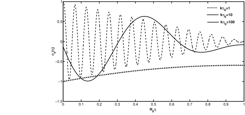
Figure 1: The variation of $\sigma_{k}(\eta)$ for three different values of $k$.

2.2   Vector modes:

We next consider the vector perturbations. For simplicity we rewrite the Einstein equation in the following form,

$$R_{\mu\nu}=T_{\mu\nu}-\frac{1}{2}g_{\mu\nu}T^{\alpha}_{\alpha}.$$ (41)

The $j-i$ components of Eq. 41 give,

$$\partial_{j}\left[V_{i}^{\prime\prime}+2\frac{a^{\prime}}{a}V_{i}^{\prime}-M_{i}^{\prime}-2\frac{a^{\prime}}{a}M_{i}\right]=0$$ (42)

and $0-i$ components may be written as,

$$\nabla^{2}(M_{i}-V_{i}^{\prime})=0\ .$$ (43)

Here we have used the Eq. 12. We make a gauge choice as $M_{i}=0$ which implies $\nabla^{2}V_{i}=0$. From Eq. 42 we get

$$\partial_{j}\left[V_{i}^{\prime\prime}+2\frac{a^{\prime}}{a}V_{i}^{\prime}\right]=0.$$ (44)

As we seek solutions whose spatial dependence is given by $\exp(i\vec{k}\cdot\vec{x})$ this implies,

$$V_{i}^{\prime\prime}-\frac{2}{\eta+C}V_{i}^{\prime} = 0,$$ (45)

where we have used Eq. 31. Hence the solution of vector mode perturbation is

$$V_{i} = C^{V}_{i}\frac{(\eta-\eta_{0})^{3}}{3}e^{i\vec{k}\cdot\vec{x}}\ ,$$ (46)

where $C^{V}_{i}$ is a constant vector. This implies that as $\eta\rightarrow\eta_{0}$, the vector perturbation dies off as $(1-\eta/\eta_{0})^{3}$.

2.3   Tensor modes:

We finally consider the tensor modes. As already mentioned we do not need to make any gauge choice to solve for the tensor mode. Using Eq. 12 the equation for the tensor modes can be written as,

$$\nabla^{2}P_{ij}-2\frac{a^{\prime}}{a}P_{ij}^{\prime}-P_{ij}^{\prime\prime}=0\ .$$ (47)

Comparing this with Eq. 38 we see that $P_{ij}$ satisfies the same equation as $A$. Hence, the solution for the tensor modes is same as that of the scalar perturbations.

3   Conclusion

We have considered a scale invariant model of gravity including an extra real scalar field. The scaling symmetry is broken by a mechanism which has some similarity to spontaneous symmetry breaking. In this case a time dependent solution of the classical equations of motion breaks the symmetry and generates all the dimensionful parameters of the theory like the gravitational constant and an effective cosmological constant. In this paper we have analyzed the stability of such a solution against small perturbations. We have shown that the symmetry breaking solution is stable against small perturbations, irrespective of their scalar, vector or tensor nature. However the exact behavior depends on the nature of the perturbation. The scalar and tensor perturbations show damped oscillations as a function of conformal time $\eta$. The vector perturbation, however, decay monotonically with conformal time. Our results establish the robustness of this mechanism to break scale invariance.

References

- [1] H. Weyl, Z. Phys. 56, 330 (1929) [Surveys High Energ. Phys. 5, 261 (1986)].
- [2] S. Deser, Annals Phys. 59, 248 (1970).
- [3] P. A. M. Dirac, Proc. Roy. Soc. Lond. A 333, 403 (1973).
- [4] D. K. Sen and K. A. Dunn, J. Math. Phys. 12, 578 (1971).
- [5] R. Utiyama, Prog. Theor. Phys. 50, 2080 (1973).
- [6] P. G. O. Freund, Annals Phys. 84, 440 (1974).
- [7] K. Hayashi, M. Kasuya and T. Shirafuji, Prog. Theor. Phys. 57, 431 (1977) [Erratum-ibid. 59, 681 (1978)].
- [8] M. Nishioka, Fortsch. Phys. 33, 241 (1985).
- [9] T. Padmanabhan, Class. Quant. Grav. 2, L105 (1985).
- [10] H. Cheng, Phys. Rev. Lett. 61, 2182 (1988).
- [11] D. Hochberg and G. Plunien, Phys. Rev. D 43, 3358 (1991).
- [12] J. T. Wheeler, J. Math. Phys. 39, 299 (1998) [arXiv:hep-th/9706214].
- [13] M. Pawlowski, Turk. J. Phys. 23, 895 (1999) [arXiv:hep-ph/9804256].
- [14] H. Nishino and S. Rajpoot, Phys. Rev. D 79, 125025 (2009) [arXiv:0906.4778 [hep-th]].
- [15] D. A. Demir, Phys. Lett. B 584, 133 (2004) [arXiv:hep-ph/0401163].
- [16] C. g. Huang, D. d. Wu and H. q. Zheng, Commun. Theor. Phys. 14, 373 (1990).
- [17] H. Wei and R. G. Cai, JCAP 0709:015 (2007) [arXiv:astro-ph/0607064].
- [18] P. Jain, S. Mitra and N. K. Singh, JCAP 0803:011 (2008) [arXiv:0801.2041 [astro-ph]].
- [19] P. K. Aluri, P. Jain and N. K. Singh, Mod. Phys. Lett. A 24, 1583 (2009) [arXiv:0810.4421 [hep-ph]].
- [20] T. Y. Moon, J. Lee and P. Oh, Mod. Phys. Lett. A 25, 3129 (2010).
- [21] F. Englert, C. Truffin and R. Gastmans, Nucl. Phys. B 117, 407 (1976).
- [22] M. Shaposhnikov and D. Zenhausern, Phys. Lett. B 671, 162 (2009) [arXiv:0809.3406 [hep-th]].
- [23] P. Jain and S. Mitra, Mod. Phys. Lett. A 24, 2069 (2009) [arXiv:0902.2525 [hep-ph]].
- [24] P. Jain and S. Mitra, Mod. Phys. Lett. A 25, 167 (2010) [arXiv:0903.1683 [hep-ph]].
- [25] P. K. Aluri, P. Jain, S. Mitra, S. Panda and N. K. Singh, Mod. Phys. Lett. A 25, 1349 (2010) [arXiv:0909.1070 [hep-ph]].
- [26] P. D. Mannheim, arXiv:0909.0212 [hep-th].
- [27] Y. Fujii, Phys. Rev. D 9, 874, (1974).
- [28] F. Cooper and G. Venturi, Phys. Rev. D 24, 3338 (1981).
- [29] W. R. Wood and G. Papini, Phys. Rev. D 45, 3617 (1992).
- [30] A. Feoli, W. R. Wood and G. Papini, J. Math. Phys. 39, 3322 (1998) [arXiv:gr-qc/9805035].
- [31] P. Jain and S. Mitra, Mod. Phys. Lett. A 22, 1651 (2007) [arXiv:0704.2273 [hep-ph]].
- [32] F. Finelli, A. Tronconi and G. Venturi, Phys. Lett. B 659, 466 (2008) [arXiv:0710.2741 [astro-ph]].
- [33] J. F. Donoghue, Phys. Rev. D 50, 3874 (1994) [arXiv:gr-qc/9405057].
- [34] J. F. Donoghue, arXiv:gr-qc/9512024.
- [35] N. Dadhich, arXiv:1006.1552.
- [36] V. Faraoni, Phys. Rev. D 70, 044037 (2004).
- [37] V. Faraoni, Phys. Rev. D 72, 061501 (2005) [arXiv:gr-qc/0509008v1].
- [38] I. Quiros, Y. Leyva, Y. Napoles, Phys. Rev. D 80, 024022 (2009) [arXiv:0906.1190].
- [39] H. Zhang, X. LiZhang, JHEP 1106:043 (2011) [arXiv:1007.3096v1].
- [40] J. Hwang, Class. Quant. Grav., 14, 1981 (1997) [arXiv:gr-qc/9605024v1]
- [41] A. Cerioni, F. Finelli, A. Tronconi, and G. Venturi, Phys. Rev. D 81, 123505 (2010) [arXiv:1005.0935].
- [42] B. A. Bassett, S. Tsujikawa, D. Wands, Rev. Mod. Phys., 78, 537 (2006) [arXiv:astro-ph/0507632v2]
- [43] D. Langlois, Cargese 2003, Particle physics and cosmology, 235 (2003) [arXiv:hep-th/0405053v1]
- [44] R. Durrer, J. Phys. Stud., 5, 177 (2001) [arXiv:astro-ph/0109522v1]
- [45] R. H. Brandenberger, Lect. Notes Phys. 646, 127-167 (2004) [arXiv:hep-th/0306071].
- [46] V. F. Mukhanov, H. A. Feldman and R. H. Brandenberger, Phys. Rept. 215, 203 (1992).
- [47] N. Straumann, Annalen Phys. 17, 609 (1997) [arXiv:0805.4500 [gr-qc]].
- [48] S. Dodelson, Modern Cosmology (Academic Press, San Diego, California, USA, 2003).
- [49] E. M. Lifshitz, J. Phys. USSR. 10, 116 (1946).
- [50] E. M. Lifshitz, I.M. Khalatnikov, Adv. Phys. 12, 185 (1963).
- [51] E. Bertschinger, In proceedings of Cosmology 2000. Instituto Superior Tecnico, Lisbon, Portuga. July 12 - 15 (2000) [arXiv:astro-ph/0101009].
- [52] J. M. Bardeen, Phys. Rev. D, 22, 1882 (1980).
- [53] C. P. Ma and E. Bertschinger, Astrophys. J. 455, 7 (1995) [arXiv:astro-ph/9506072].
- [54] A. Riotto, arXiv:hep-ph/0210162.
- [55] S. Weinberg, Cosmology (Oxford University Press, New York, USA, 2008).