Coherent spectrum rearrangement in graphene: extra nodal point and impurity band with anomalous dispersion

Abstract

It is demonstrated that an extra nodal point and a domain with anomalous dispersion are present in the spectrum of charge carriers in graphene, when the concentration of weakly bound impurities exceeds a certain critical value, determined by the spatial overlap of individual impurity states. Corresponding spectrum rearrangement is shown to be of the cross type.

I Introduction

Chemical functionalization of graphene is currently a rapidly developing field of research.gem ; buh By depositing various atoms, molecules and chemically active groups on graphene, it is possible to tune up its properties according to specific technical applications. Undoubtedly, transport properties of graphene are decisive for its future in microelectronic devices of the new generation. With respect to the transport properties, adatoms should be viewed, first of all, as a sort of defects, which can significantly alter the spectrum of charge carriers and lead to the localization of states. It was demonstrated experimentally that ion bombardmentfuh , deposition of atomic hydrogeneli or fluorinesav opens a mobility gap in the electron spectrum of graphene and triggers the metal-insulator transition, just as it happens in conventional systems with massive carriers. The opening of the mobility gap in graphene is attributed to the presence of impurity resonance states in the Dirac point vicinity. Moreover, it became evident that some amount of resonant defects is always present in graphene obtained by the micromechanical cleavage process.gei It follows from theoretical studies of generic models for adsorbed atoms that such defects should considerably modify the electron density of states and affect the conductivity of graphene.fal ; weh ; kat ; net ; ihn However, only those cases were examined, in which impurity levels of adatoms were strongly bound to the host.

Lifshitz defects (vacancies including), which do nothing to the system but change effective potentials on lattice sites occupied by them, bear a lot of similarity to strongly bound impurity centers.mit Albeit such defects are capable in producing resonance states in the Dirac point vicinity, the corresponding resonances are of a reduced integral intensity, and the subsequent spectrum rearrangement has a diffuse, anomalous character, which is inherent in low-dimensional systems.sl ; psl This type of the spectrum rearrangement is characterized by the presence of two non-overlapping dispersion branches in the spectrum, which are separated by a mobility gap. At that, the density of states inside this gap can considerably exceed the one in the host.psl

However, there is a different opportunity: spectra of elementary excitations in tree-dimensional systems (and in low-dimensional ones as well) can undergo a rearrangement of the coherent (cross) type with increasing the amount of impurities.ilp The renormalized dispersion resulting from the spectrum rearrangement of this type looks similar to the hybridization between the host branch and the dispersionless branch that corresponds to the impurity state energy. Namely, two overlapping branches develop in the spectrum of a disordered system. As a consequence, two different energies of quasiparticles correspond to each wave vector. These dispersion branches are separated by a true gap, which is gradually broadening with increasing the impurity concentration. The cross-type spectrum rearrangement is usually accompanied by strong single-impurity resonances, which appear in low-dimensional systems only for weakly bound impurities. Thus, we examine below possible changes in the electron spectrum of graphene, which can occur under an increase in the impurity concentration, when impurity levels are weakly bound to the host.

II Impurity model

When dealing with $\pi$-electron bands of graphene within the tight-binding approximation, it is usually sufficient to take into consideration only matrix elements between nearest neighbors in the honeycomb lattice:rmf

$${\bm{H}}={\bm{H}}_{0}+{\bm{H}}_{im},\quad{\bm{H}}_{0}=\frac{1}{\sqrt{\pi\sqrt{3}}}\sum\nolimits^{\prime}c_{{\bm{n}}\alpha}^{\dagger}c_{{\bm{m}}\beta}^{\phantom{\dagger}},$$ (1)

where ${\bm{H}}_{0}$ is the dimensionless host Hamiltonian, ${\bm{H}}_{im}$ is the impurity perturbation, vector ${\bm{n}}$ runs over lattice cells, indices $\alpha$ and $\beta$ enumerate sublattices, $c_{{\bm{n}}\alpha}^{\dagger}$ and $c_{{\bm{n}}\alpha}^{\phantom{\dagger}}$ are the creation and annihilation Fermi operators at the corresponding lattice site, and the prime at the sum sign indicates that $\bm{n}\alpha\neq\bm{m}\beta$. For the sake of simplicity we choose the energy unit in such a way that the transfer integral $t=1/\sqrt{\pi\sqrt{3}}$. Since its magnitude in graphene is taken to be around $2.7$ eV in most cases, the adopted energy unit is about $6.3$ eV.

If chemisorbed atoms play the role of defects, even a minimal impurity model should contain, in a general case, a possibility for the electron transfer from the host to some energy level that belongs to the adsorbed atom. This task is fulfilled by the well-known Fano-Anderson impurity model,fan which was adopted in quite a few studies devoted to adatoms on graphene.fal ; weh ; kat ; net ; gru On the assumption that impurities are deposited without any spatial correlation, we arrive at the following impurity part of the Hamiltonian:

$${\bm{H}}_{im}=\sum\eta_{{\bm{n}}\alpha}^{\phantom{\dagger}}\left[\varepsilon_{0}d_{{\bm{n}}\alpha}^{\dagger}d_{{\bm{n}}\alpha}^{\phantom{\dagger}}+(\gamma c_{{\bm{n}}\alpha}^{\dagger}d_{{\bm{n}}\alpha}^{\phantom{\dagger}}+h.c.)\right],$$ (2)

where dimensionless $\gamma$ is the hybridization between the adatom and the host, $\varepsilon_{0}$ is the bare energy of the adatom level, $d_{{\bm{n}}\alpha}^{\dagger}$ and $d_{{\bm{n}}\alpha}^{\phantom{\dagger}}$ are the creation and annihilation operators at this level, the variable $\eta_{{\bm{n}}\alpha}$ takes the value of 1 with the probability $c$ or the value of 0 with the probability $1-c$, and $c$ is the impurity concentration.

By eliminating wavefunction amplitudes at adatoms from the stationary Shrödinger equation for the operators (1) and (2), the problem can be reduced to a more simple form with

$${\bm{H}}_{im}=V\sum\limits_{{\bm{n}}\alpha}\eta_{{\bm{n}}\alpha}^{\phantom{\dagger}}c_{{\bm{n}}\alpha}^{\dagger}c_{{\bm{n}}\alpha}^{\phantom{\dagger}},\quad V=\frac{|\gamma|^{2}}{\varepsilon-\varepsilon_{0}}$$ (3)

A conclusion on the presence of a resonance state for an isolated impurity can be made based on the single-site $T$-matrix,

$$\tau(\varepsilon)=\frac{V}{1-g_{0}(\varepsilon)V}=\frac{|\gamma|^{2}}{\varepsilon-\varepsilon_{0}-|\gamma|^{2}g_{0}(\varepsilon)},$$ (4)

where $g_{0}(\varepsilon)$ is the diagonal element of the host Green’s function,

$${\bm{g}}=\frac{1}{\varepsilon-{\bm{H}}_{0}},$$ (5)

taken in the site representation. The required diagonal element can be approximated in a vicinity of the Dirac point ($\varepsilon=0$) as follows:

$$g_{0}(\varepsilon)\approx 2\varepsilon\ln(|\varepsilon|)-i\pi|\varepsilon|,\quad|\varepsilon|\ll 1.$$ (6)

Substituting this expression into Eq. (4) and taking into account that logarithm is a slowly varying function, we have:

$$\tau(\varepsilon)=\frac{|\gamma_{ef}|^{2}}{\varepsilon-\varepsilon_{ef}+i\pi|\gamma_{ef}|^{2}|\varepsilon|},$$ (7)

where the effective hybridization and the effective energy of the impurity level are introduced:

$$|\gamma_{ef}|^{2}=\frac{|\gamma|^{2}}{D},\,\varepsilon_{ef}=\frac{\varepsilon_{0}}{D},$$

$$D=1-2|\gamma|^{2}\left(\ln|\varepsilon_{r}|+1\right).$$ (8)

It immediately follows from Eq. (7) that $\varepsilon_{ef}\equiv\varepsilon_{r}$, i.e. corresponds to the energy of a possible single-impurity resonance.

This resonance can be considered as a well-defined, when its damping is significantly less than the energy interval between $\varepsilon_{r}$ and the closest van Hove singularity of the host spectrum. In the case under consideration, the role of such singularity is played by the Dirac point. Thus, the mentioned condition for the appearance of a well-defined resonance is reduced to the inequality:

$$\delta\equiv\pi|\gamma_{ef}|^{2}\ll 1,$$ (9)

where $\delta$ is the small parameter that will be used further on. It is evident, that the inequality (9) is automatically satisfied at $|\gamma|\ll 1$. Thus, a well-defined resonance state is always present in a system with Dirac-like dispersion, when the impurity level is weakly bound and the resonance energy is located close to the Dirac point. For a relatively large hybridization constant, $|\gamma|\gtrsim 1$, the inequality (9) takes the form:

$$\frac{\pi}{2\left|\ln|\varepsilon_{r}|+1\right|}\ll 1,$$ (10)

which can be satisfied only at a close proximity of the resonance energy to the Dirac point, and coincides with the corresponding condition for Lifshitz impurity centers.sl One can expect that at $|\gamma|\gtrsim 1$ the spectrum rearrangement, for the most part, also proceeds according to the anomalous scenario, which already has been examined in detail for Lifshitz impurities.sl ; psl Therefore, we are focused on the opposite case of weakly bound impurities ($|\gamma|\ll 1$) below. In other words, the hybridization parameter has to be smaller than the transfer integral magnitude in the host.

III Coherent spectrum rearrangement

At low impurity concentrations, $c\ll 1$, the spectrum rearrangement can be analyzed by means of the modified propagator method.lang Within this approach, the self-energy $\sigma(\varepsilon)$, which approximates the averaged over impurity distributions Green’s function of a disordered system

$${\bm{G}}=\left<\frac{1}{\varepsilon-{\bm{H}}}\right>\approx\frac{1}{\varepsilon-\sigma(\varepsilon)-{\bm{H}}_{0}},$$ (11)

is determined self-consistently:

$$\sigma(\varepsilon)=\frac{c|\gamma|^{2}}{\varepsilon-\varepsilon_{0}-|\gamma|^{2}g_{0}[\varepsilon-\sigma(\varepsilon)]}.$$ (12)

We would like to remind that this method does not work satisfactorily in all spectral intervals of a disordered system.ilp Due to increased scatterings on impurity clusters, concentration broadening areas are formed nearby singular points of the spectrum. Inside these areas the approximation (12) is not valid and states turn out to be localized. Thus, in order to locate such areas and to determine their widths, it is often enough to employ the standard Ioffe-Regel criterion:iof

$$|\tilde{\varepsilon}(\varepsilon)|\equiv|\varepsilon-\operatorname{Re}\sigma(\varepsilon)|\gg-\operatorname{Im}\sigma(\varepsilon),$$ (13)

where $\tilde{\varepsilon}(\varepsilon)$ is the renormalized energy. According to the approximation (11), it specifies the renormalized dispersion relation in a disordered system inside those spectral domains, which are occupied by extended states:

$$\tilde{\varepsilon}(\varepsilon)=\varepsilon(\bm{k}),$$ (14)

where $\varepsilon(\bm{k})$ is the host dispersion. It is well known that the Hamiltonian (1) yields the linear dispersion for free charge carriers, when the wave vector is counted from one of the two inequivalent Dirac points in the Brillouin zone:

$$\varepsilon(\bm{k})\approx\pm v_{F}k,\qquad v_{F}=\frac{a}{2}\sqrt{\frac{\sqrt{3}}{\pi}},$$ (15)

where $a$ is the honeycomb lattice constant.

Let’s assume that the spectrum rearrangement has occurred already. After the rearrangement, the spectrum of the disordered system should undergo a cardinal change. We are going to pay attention only to states that remain extended despite the presence of disorder and to make several estimations that should help to sketch up the overall structure of the rearranged spectrum. Due to the singular character of the impurity perturbation, the distortion of the spectrum is most pronounced around the resonance energy $\varepsilon_{r}$.

Taking into account expressions (6-8), and (12), the imaginary part of the self-energy can be approximated as follows:

$$\operatorname{Im}\sigma(\varepsilon)\approx-\frac{c\pi|\gamma_{ef}|^{4}|\tilde{\varepsilon}(\varepsilon)|}{(\varepsilon-\varepsilon_{r})^{2}+(\pi|\gamma_{ef}|^{2}\tilde{\varepsilon}(\varepsilon))^{2}},$$ (16)

when the condition (13) holds, and, consequently, the corresponding states can be treated as extended ones. While remaining inside the domain of extended states, it is possible, regardless of the strong impurity scattering near the resonance energy, to go further and to omit the second term in the denominator of (16) (justification of this approximation will be provided below). Then, the inequality (13) in a vicinity of $\varepsilon_{r}$ can be rewritten as:

$$|\tilde{\varepsilon}(\varepsilon)|\gg\frac{c\pi|\gamma_{ef}|^{4}|\tilde{\varepsilon}(\varepsilon)|}{(\varepsilon-\varepsilon_{r})^{2}},$$ (17)

which turns to

$$|\varepsilon-\varepsilon_{r}|\gg\sqrt{\pi c}|\gamma_{ef}|^{2}\equiv\Delta_{r}.$$ (18)

Thus, the width of the concentration broadening area of the impurity resonance $\Delta_{r}$ is increasing proportional to $\sqrt{c}$, i.e. behaves like the width of the mobility gap, which opens under the anomalous spectrum rearrangement in graphene with Lifshitz impurities.sl However, it is worth noticing that, in comparison with the case of Lifshitz defects, the width $\Delta_{r}$ contains the small parameter of the problem $|\gamma_{ef}|^{2}$ as a multiplier. Similarly, within the same approximations, we have inside domains of extended states that

$$\tilde{\varepsilon}(\varepsilon)\approx\varepsilon-\frac{c|\gamma_{ef}|^{2}}{\varepsilon-\varepsilon_{r}}.$$ (19)

The renormalized dispersion relation $\tilde{\varepsilon}(\bm{k})$, which is depicted in Fig. 1, can be obtained from Eqs. (14) and (19) as a solution of the quadratic equation,

$$\tilde{\varepsilon}(\bm{k})\approx\frac{1}{2}\Bigl{\{}\varepsilon_{r}+\varepsilon(\bm{k})\pm\sqrt{[\varepsilon_{r}-\varepsilon(\bm{k})]^{2}+4c|\gamma_{ef}|^{2}}\ \Bigr{\}}.$$ (20)

Obviously, positions of nodal points, i.e. those points at which dispersion cones are touching each other by their vertices, are determined in the rearranged spectrum by the condition $\varepsilon(\bm{k})=0$. Thus, it follows from the dispersion law (20) that there should be a second (impurity) nodal point with the energy

$$\varepsilon_{nod}\approx\frac{1}{2}\Bigl{(}\varepsilon_{r}+\sqrt{\varepsilon_{r}^{2}+4c|\gamma_{ef}|^{2}}\ \Bigr{)},$$ (21)

where we also assumed that $\varepsilon_{r}>0$ without loosing generality. At low impurity concentrations,

$$\varepsilon_{nod}\approx\varepsilon_{r}+\Delta_{nod},\quad\Delta_{nod}\approx\frac{c|\gamma_{ef}|^{2}}{\varepsilon_{r}},\$$ (22)

moreover, $\Delta_{nod}\ll\varepsilon_{r}$. On the other hand, one can speak about the appearance of the extra nodal point in the spectrum only in the case, when it lies outside the concentration broadening area of the impurity resonance, i.e.

$$\Delta_{nod}\gg\Delta_{r}.$$ (23)

In essence, the condition (23) determines the critical concentration of the coherent spectrum rearrangement,

$$c_{csr}\sim\pi\varepsilon_{r}^{2}.$$ (24)

It is not difficult to see that this magnitude agrees with quick-and-dirty estimates for the critical concentration, which are based on the mutual spatial overlap of individual impurity states. Namely, the period of spatial oscillations of the host Green’s function in graphene determines the characteristic radius of the single-impurity state: $r_{imp}\sim a\varepsilon_{r}^{-1}$. With increasing the impurity concentration, the average distance between impurities $\bar{r}\sim ac^{-1/2}$ is gradually decreasing. Both lengths become equal at $c\sim\varepsilon_{r}^{2}$, which is in accord with the relation (24).psl ; mit

As it follows from Eqs. (18) and (19), the absolute value of the renormalized energy $\tilde{\varepsilon}(\varepsilon)$ is of the order of $\sqrt{c/\pi}$ at the boundaries of the concentration broadening area located at the resonance energy, and, according to the relation (24), far exceeds $\varepsilon_{r}$ in the rearranged spectrum. The corresponding maximum value of the wave vector $k_{max}$ (see Fig. 1) that is reached at the boundaries of the concentration broadening area appears to be of the order of the inverse mean distance between impurities, as it would be expected:

$$k_{max}\sim\frac{2}{a}\sqrt{\frac{c}{\sqrt{3}}}.$$ (25)

By substituting the magnitude $\sqrt{c/\pi}$ in place of $\tilde{\varepsilon}(\varepsilon)$ in the denominator of Eq. (16), one can easily verify that the second term is small in comparison with the first one by virtue of the inequality (18). This justifies the omission of the second term in the denominator of Eq. (16) for the extended states.

When energy is crossing $\varepsilon_{r}$, the corresponding $\tilde{\varepsilon}(\varepsilon)\approx c|\gamma_{ef}|^{2}/(\varepsilon-\varepsilon_{r})$ changes its sign. In this way a spectral domain with anomalous dispersion develops between $\varepsilon_{r}$ and $\varepsilon_{nod}$ (see Fig. 1(a)). With respect to the valence band (as it appears in the Figure), this domain can be considered as an impurity band filled with extended (itinerant) states. Because of the particle-hole symmetry of the host spectrum, this impurity band fits exactly inside the gap that opens under the cross-type spectrum rearrangement of the conduction band. At that, the impurity band formation occurs simultaneously for both Dirac cones in the Brillouin zone of graphene.

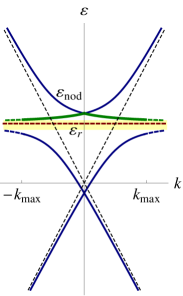
(a) $c<c_{*}$

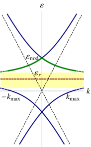
(b) $c>c_{*}$

Figure 1: (Color online) Sketches of the dispersion of charge carriers in graphene with weakly bound impurities after the cross-type spectrum rearrangement drawn according to Eq. (20): (a) $c_{csr}<c<c_{*}$, the Fermi velocity at the impurity nodal point is significantly reduced; (b) $c_{*}<c\ll 1$, the Fermi velocity at the impurity nodal point is comparable to the one in the host system. The host dispersion is shown by the dashed line. Branches with the anomalous dispersion are given by the thick (green) solid line. The concentration broadening area is marked by the (yellow) shade.

It follows from Eq. (21) and the definition (22) that at

$$c\gg c_{*}\sim\frac{\varepsilon_{r}^{2}}{|\gamma_{ef}|^{2}}$$ (26)

the width of the anomalous dispersion domain $\Delta_{nod}$ becomes of the order of $\sqrt{c}|\gamma_{ef}|$, and thus scales differently with the impurity concentration. Since $c_{csr}/c_{*}\sim\delta$, the small parameter, which was defined by Eq. (9), this characteristic concentration always exceeds the critical concentration of the spectrum rearrangement. At the onset of the spectrum rearrangement, the quantity $\Delta_{r}$ has a square root dependence on $c$, while $\Delta_{nod}$ has a linear one, which ensures its leading growth. By contrast, both widths have a square root dependence on the impurity concentration at $c>c_{*}$, while their ratio remains nearly constant:

$$\frac{\Delta_{r}}{\Delta_{nod}}\sim\sqrt{\delta},\quad c>c_{*}.$$ (27)

In addition, the width of the spectral domain with anomalous dispersion $\Delta_{nod}$ exceeds $|\varepsilon_{r}|$ at $c>c_{*}$ (see Fig. 1(b)).

The Fermi velocity $\tilde{v}_{F}$ at the extra nodal point $\varepsilon_{nod}$ can be expressed through the Fermi velocity of the host $v_{F}$ by means of Eq. (20):

$$\frac{\tilde{v}_{F}}{v_{F}}=\frac{1}{v_{F}}\left.\frac{d\,\tilde{\varepsilon}(\bm{k})}{d\,k}\right|_{k=0}=\left.\frac{d\,\tilde{\varepsilon}(\bm{k})}{d\,\varepsilon(\bm{k})}\right|_{\varepsilon(\bm{k})=0}\approx\\ \frac{1}{2}\left[1-\left(1+4\frac{c}{c_{*}}\right)^{-1/2}\right],$$ (28)

where the plus sign was chosen for the square root term in Eq. (20). It is easy to see from the ratio (28) that the Fermi velocity $\tilde{v}_{F}$ is reduced in $c/c_{*}$ times at $c\ll c_{*}$ in comparison with the one of the host. As a result, it can be difficult to observe the branch with the anomalous dispersion in real experiments. However, this velocity is gradually approaching $v_{F}/2$ for $c\gg c_{*}$, which eliminates indicated difficulties. Because the Fermi velocity near $\varepsilon_{nod}$ varies in several times, and the width of the anomalous dispersion domain varies with the impurity concentration according to a different law, the characteristic concentration $c_{*}$ separates two dissimilar regimes of the coherent spectrum rearrangement.

The width $\Delta_{r}$ is of the order of $\delta|\varepsilon_{r}|$ at $c\sim c_{csr}$, i.e. is substantially smaller than the interval between $\varepsilon_{r}$ and the initial position of the host Dirac point. This relationship becomes reversed at

$$c>c_{sym}\sim\frac{\varepsilon_{r}^{2}}{\pi|\gamma_{ef}|^{4}}\sim\frac{c_{*}}{\delta}\sim\frac{c_{csr}}{\delta^{2}}.$$ (29)

Therefore, the asymmetry, which is present in the spectrum due to the nonzero energy of the impurity resonance state, is effectively smeared out, when the impurity concentration is that high.

In the first approximation, as it follows from Eqs. (12) and (22), the impurities under consideration behave in a close vicinity of $\varepsilon_{nod}$ at $c_{csr}<c<c_{*}$ like Lifshitz defects with the on-site impurity perturbation $v_{L}\approx\varepsilon_{r}/c$. According to the results obtained in Ref. sl, , the critical concentration of the anomalous spectrum rearrangement for such defects can be roughly estimated as $c_{asr}\sim 1/v_{L}^{2}$. Thus, the condition $c<c_{asr}\sim c^{2}/\varepsilon_{r}^{2}$ should be satisfied for the system to remain in the unrearranged regime. This condition reduces to $c>c_{csr}$, which is, for certain, fulfilled. It was demonstrated in Ref. sl, that in such a case the concentration broadening area of the Dirac point is exponentially small as compared to the bandwidth. Thus, its presence can be, to a known extent, overlooked.

Similarly, the effective Lifshitz impurity perturbation in the vicinity of $\varepsilon_{nod}$ is $v_{L}\sim|\gamma_{ef}|/\sqrt{c}$ at $c>c_{*}$, and the exponential smallness of the corresponding concentration broadening area is guaranteed by the inequality $c<c/|\gamma_{ef}|^{2}$, which is fulfilled on account of the condition (9).

The host Dirac point, which is always present in the spectrum, is also shifted from its initial position due to the effect of impurities. As it directly follows from Eq. (20), the magnitude of this shift is about $-c|\gamma_{ef}|^{2}/|\varepsilon_{r}|$ at low impurity concentrations, which agrees with the width of the anomalous dispersion domain at $c>c_{csr}$. At that, this shift occurs in a direction opposite to the concentration displacement of $\varepsilon_{nod}$ from $\varepsilon_{r}$.

For $c<c_{*}$, the effective magnitude of the impurity perturbation $v_{L}\sim-|\gamma_{ef}|^{2}/|\varepsilon_{r}|$ in a vicinity of the shifted host Dirac point, and the corresponding critical concentration $c_{asr}\sim\varepsilon^{2}_{r}/|\gamma_{ef}|^{4}$. The inequality $c_{*}<c_{asr}$ is again met in view of the condition (9). Thus, the width of the concentration broadening area remains once more exponentially small. At $c>c_{*}$, the Dirac point shift is $\sim\sqrt{c}|\gamma_{ef}|$ by the absolute value, and the analysis of its concentration broadening can be performed in much the same way as it was done above for the extra nodal point vicinity.

IV Conclusion

To summarize, with increasing the concentration of weakly bound impurity centers, which yield well-defined resonance states, the electron spectrum of graphene undergoes the coherent cross-type spectrum rearrangement. In contrast to the already known cases of the coherent spectrum rearrangement, it manifests the impurity nodal point in the spectrum and the impurity band with the anomalous dispersion. In addition, it features a concentration broadening area, or a mobility gap, around the impurity resonance energy, and thus, when the Fermi level position in the system is controlled by, for example, the gate voltage, it should be possible to observe a metal-insulator transition on Fermi level’s entering the mobility gap, and then a re-entrant insulator-metal transition on its leaving. For Lifshitz defects, the mobility gap is narrower than the bandwidth in $\sim\sqrt{c}$ times. In contrast, the mobility gap width for weakly bound defects $\Delta_{r}$ contains additional small parameter as a multiplier (see the inequality (18)). Therefore, weakly bound impurities are more favorable for the experimental study of the re-entrant insulator-metal transition in graphene.

- (1) A. K. Geim, Science 324, 1530 (2009).
- (2) D. W. Boukhvalov, and M. I. Katsnelson, J. Phys.: Condens. Matter 21 344205 (2009).
- (3) J.-H. Chen,W. G. Cullen, C. Jang, M. S. Fuhrer, and E. D. Williams, Phys. Rev. Lett. 102, 236805 (2009).
- (4) A. Bostwick, J. L. McChesney, K. V. Emtsev, T. Seyller, K. Horn, S. D. Kevan, and E. Rotenberg, Phys. Rev. Lett. 103, 056404 (2009).
- (5) F. Withers, M. Dubois, and A. K. Savchenko, Phys. Rev. B 82, 073403 (2010).
- (6) Z. H. Ni, L. A. Ponomarenko, R. R. Nair, R. Yang, S. Anissimova, I. V. Grigorieva, F. Schedin, Z. X. Shen, E. H. Hill, K. S. Novoselov, and A. K. Geim, Nano Lett. 10, 3868 (2010).
- (7) J. P. Robinson, H. Schomerus, L. Oroszlany, and V. I. Fal ko, Phys. Rev. Lett. 101, 196803 (2008).
- (8) T. O. Wehling, S. Yuan, A. I. Lichtenstein, A. K. Geim, and M. I. Katsnelson Phys. Rev. Lett. 105, 056802 (2010).
- (9) S. Yuan, H. De Raedt, and M. I. Katsnelson, Phys. Rev. B 82, 115448 (2010).
- (10) A. Ferreira, J. Viana-Gomes, J. Nilsson, E. R. Mucciolo, N. M. R. Peres, and A. H. Castro Neto, Phys. Rev. B 83, 165402 (2011).
- (11) S. Ihnatsenka, and G. Kirczenow, Phys. Rev. B 83, 245442 (2011).
- (12) Yu. V. Skrypnyk, and V. M. Loktev, Phys. Rev. B 83, 085421 (2011).
- (13) Yu. V. Skrypnyk, and V. M. Loktev, Phys. Rev. B 73, 241402(R) (2006).
- (14) S. S. Pershoguba, Yu. V. Skrypnyk, and V. M. Loktev, Phys. Rev. B 80, 214201 (2009).
- (15) M. A. Ivanov, V. M. Loktev, and Yu. G. Pogorelov, Phys. Rep. 153, 209 (1987).
- (16) A. H. Castro Neto, F. Guinea, N. M. R. Peres, K. S. Novoselov, and A. K. Geim, Rev. Mod. Phys. 81, 109 (2009).
- (17) U. Fano, Phys. Rev. 124, 1866 (1961).
- (18) M. Farjam, D. Haberer, and A. Grüneis, Phys. Rev. B 83, 193411 (2011).
- (19) R. W. Davies, and J. S. Langer, Phys. Rev. 131, 163 (1963).
- (20) A. F. Ioffe, and A. R. Regel, Prog. Semicond. 4, 237 (1960).