Driving the resonant quantum kicked rotor via extended initial conditions

Abstract

We study the resonances of the quantum kicked rotor subjected to an extended initial distribution. For the primary resonances we obtain the dispersion relation for the map of this system. We find an analytical dependence of the statistical moments on the shape of the initial distribution. For the secondary resonances we obtain numerically a similar dependence. This allows us to devise an extended initial condition which produces an average angular momentum pointing in a preset direction which increases with time with a preset ratio.

1 Introduction

The quantum kicked rotor (QKR), can be considered a cornerstone in the study of chaos at the quantum level CCI79 . Both in theoretical and experimental terms, this topic is a matter of permanent attention Schomerus1 ; Schomerus2 ; Currivan ; Sandgrove ; Saunders ; Halkyard . An experimental realization of the quantum kicked top (a variant of the QKR) has been recently reported Chaudhury and used to study the signatures of quantum chaos. The behavior of the QKR has two characteristic modalities: dynamical localization and ballistic spreading of the variance in resonance Izrailev . These behaviors are quite different and have no classical analog. They depend on the relationship between the characteristic time of the free rotor and the period associated to the kick. When the dimensionless period of the kick, $T$, is an irrational multiple of $2\pi$ the average energy of the system grows in a diffusive manner for a short time and afterwards dynamical localization appears. In this case, the angular momentum distribution is characterized by an exponential decay. When $T$ is a rational multiple of $2\pi$ the behavior of the system is resonant with a ballistic spreading. In this case the angular momentum distribution evolves from the initial one in such away that its standard deviation has the time dependence $\sigma(t)\sim t$. This quantum behavior is similar to the optical Talbot effect Goodman ; Patorski in the time dimension.

The QKR has been experimentally realized through a dilute sample of ultra-cold atoms exposed to a one-dimensional spatially periodic optical potential that is pulsed on periodically in time (to approximate a series of delta function kicks). The quantum resonances and the dynamical localization have been experimentally observed in refs. Moore ; Bharucha ; Raizen ; Kanem . However with the aim of the present paper in mind, it is interesting to highlight the work developed in refs. Currivan ; Sandgrove ; Saunders ; Halkyard , where the influence of an initial momentum on the appearance of quantum resonances in the QKR is explored experimentally establishing the dependence of the quantum resonances on the initial velocity of the atoms. In ref.Currivan , the authors showed a sinusoidal dependence of the energy on the initial momentum for two kicks, and a more complex behavior with the same period at four kicks. They also proposed to use the momentum dependence of the kicked rotor to select narrow parts of an initial momentum distribution. In refs.Saunders ; Halkyard the dynamics of a dilute atomic gas kicked periodically has been studied. There, the authors obtain analytical expressions for the time evolution of the moments of momentum for extended initial conditions, corresponding to the Boltzmann distribution of an ideal gas.

On the other hand, in a recent paper German , the evolution of initially extended distributions in the quantum walk (QW) on the line was studied. In that work, through an analysis of the dispersion relation of the process and the introduction of extended initial conditions, continuous wave equations are derived. In particular, for a class of initial conditions, the evolution is dictated by the Schrödinger equation of a free particle. This allows to devise an initially extended condition leading to a uniform probability distribution whose width increases linearly with time, and with increasing homogeneity. Additionally, in some previous works alejo1 ; alejo2 ; alejo5 ; alejo6 ; auyuanet ; victor ; monva a parallelism between the behavior of the QKR and a generalized form of the QW was developed, showing that these models have similar dynamics. In the same line of thought of reference German , in this paper we study the dependence of the QKR in resonance with extended initial conditions. In particular we obtain, analytically, a dispersion relation that controls not only the velocity of the wavepacket, but also the evolution of its shape as a function of time.

The paper is organized as follows: In the next section we present a brief revision of the QKR equations, in the third section we present the dispersion relation of the map and the group velocity, in section $4$ we study the behavior of the system under extended initial conditions, in section $5$ numerical results are presented for the secondary resonances, and in the last section we draw the conclusions.

2 Quantum kicked rotor

The QKR is one of the simplest and best investigated quantum models whose classical counterpart displays chaos. The Hamiltonian has the following shape

$$\mathbf{H}(t)=\frac{\mathbf{L}^{2}}{2I}+K\cos\mathbf{\Theta}\sum_{n=1}^{\infty}\delta(t-nT),$$ (1)

where $K$ is the strength parameter, $I$ is the moment of inertia of the rotor, $\mathbf{L}$ the angular momentum operator, $T$ the kick period and $\mathbf{\Theta}$ the angular position operator. Given the delta function appearing in eq.(1), the external kicks occur at times $t=nT$ with $n$ integer. The index $n$ will be equivalent to time in units of $T$ and the two operators $\mathbf{L}$ and $\mathbf{\Theta}$ satisfy the canonical commutation rule

$$[\mathbf{L},\mathbf{\Theta}]=-i\hbar.$$ (2)

In the angular momentum representation, $\mathbf{L}|\mathit{l}\rangle=\mathit{l}\hbar|\mathit{l}\rangle$, the wavevector is

$$|\Psi(n)\rangle=\sum_{\mathit{l}=-\infty}^{\infty}a_{\mathit{l}}(n)|\mathit{l}\rangle$$ (3)

and the angular momentum and energy are

$$L(n)=\left\langle\Psi\right|\mathbf{L}\left|\Psi\right\rangle=\hbar\sum_{\mathit{l}=-\infty}^{\infty}\mathit{l}\left|a_{\mathit{l}}(n)\right|^{2},$$ (4)

$$E(n)=\left\langle\Psi\right|\mathbf{H}\left|\Psi\right\rangle=\varepsilon\sum_{\mathit{l}=-\infty}^{\infty}\mathit{l}^{2}\left|a_{\mathit{l}}(n)\right|^{2},$$ (5)

where $\varepsilon=\hbar^{2}/2I$. The evolution operator $U$ is built from the Hamiltonian eq.(1). Then the unitary dynamics of the system is described by

$$|\Psi(n+1)\rangle=\mathbf{U}|\Psi(n)\rangle.$$ (6)

Substituting eq.(3) in eq.(6) and projecting over the angular momentum state $|l\rangle$, the dynamical equation for the amplitudes $a_{\mathit{l}}$ is determined

$$a_{\mathit{l}}(n+1)=\sum_{j=-\infty}^{\infty}U_{\mathit{l}j}a_{j}(n),$$ (7)

where the matrix elements of operator $\mathbf{U}$ are CCI79

$$U_{\mathit{l}j}=i^{-(j-\mathit{l})}e^{-ij^{2}\varepsilon T/\hbar}\,J_{j-\mathit{l}}(\kappa),$$ (8)

$J_{\mathit{l}}$ being the $\mathit{l}$th order cylindrical Bessel function and its argument the dimensionless kick strength $\kappa\equiv K/\hbar$. The resonance condition does not depend on $\kappa$ and takes place when the frequency of the driving force is commensurable with the frequencies of the free rotor. Inspection of eq.(8) shows that the resonant values of the scale parameter $\tau\equiv\varepsilon T/\hbar$ are the set of the rational multiples of $2\pi$, $\tau=2\pi$ $p/q$. In what follows we assume that the resonance condition is satisfied and therefore the evolution operator depends on $\kappa$, $p$ and $q$. We call a resonance primary when $p/q$ is an integer and secondary when it is not.

3 The dispersion relation and the group velocity

We shall consider the primary resonances $p/q=1$ and search for the solution of eq.(7) with the help of discrete Fourier analysis. We define the discrete Fourier transform of $a_{\mathit{l}}(n)$ as

$$\widetilde{a}_{\theta}(n)\equiv\sum_{l}e^{i(\theta\mathit{l}+\omega n)}a_{\mathit{l}}(n),$$ (9)

where $\omega$ will be determined as a function of $\theta$. Eq.(9) can be inverted to obtain

$$a_{\mathit{l}}(n)=\frac{1}{2\pi}\int_{-\pi}^{+\pi}\widetilde{a}_{\theta}(n)e^{-i(\theta\mathit{l}+\omega n)}d\theta.$$ (10)

Substituting eq.(10) in eq.(7) and using the identity Gradshteyn

$$e^{-i\kappa\cos\theta}=\sum_{j=-\infty}^{\infty}i^{-j}e^{-i\theta j}\,J_{j}(\kappa),$$ (11)

the following dispersion relation between $\omega$ and $\theta$ is obtained

$$\omega=\kappa\cos\theta.$$ (12)

Therefore, the group velocity of the system is

$$v_{g}\equiv\frac{d\omega}{d\theta}=-\kappa\sin\theta.$$ (13)

Eqs.(12) and (13) allow us to make simple but relevant predictions about the QKR dynamics. In particular, from eq.(13) it results that the group velocity will be maximum, $v_{g}=\kappa$, if $\theta=\frac{2m+1}{2}\pi$ and minimum, $v_{g}=0$, if $\theta=m\pi$ with $m=0,\pm 1,\pm 2,...$. If the initial state is a wavepacket close to some eigenfunction

$$a_{\mathit{l}}(0)=f(\mathit{l})e^{i\theta_{0}\mathit{l}},$$ (14)

where $f(\mathit{l})$ is a smooth function of $\mathit{l}$ and the value of $\theta_{0}$, the initial angular position, determines the velocity of the wavepacket. If $\theta_{0}=0$ a sufficiently extended wavepacket should stay at rest because $v_{g}=0$, while if $\theta_{0}=\pm\pi/2$ it should move with maximum velocity $v_{g}=\pm\kappa$. In order to verify this statement, in the next section we choose the initial condition as

$$a_{\mathit{l}}(0)=\left[\frac{1}{\sigma_{0}\sqrt{2\pi}}\exp{\ (-\frac{\mathit{l}^{2}}{2{\sigma_{0}}^{2}})}\right]^{\frac{1}{2}}e^{i\theta_{0}\mathit{l}},$$ (15)

where $\sigma_{0}$ is the standard deviation of the initial distribution. We shall then calculate the average momentum and energy obtained from this initial condition.

4 Moments with extended initial conditions

In the case of the primary resonances, eq.(7) is solved CCI79 using the recursion relation satisfied by the Bessel functions. The general solution can be written as

$$a_{\mathit{l}}(n)=\sum\limits_{j=-\infty}^{\infty}\left(-i\right)^{\mathit{l}-j}a_{j}(0)\,J_{\mathit{l}-j}(n\kappa),$$ (16)

where $a_{j}(0)$ are the initial amplitudes. The probability distribution at time $n$ is given by

$$P_{\mathit{l}}(n)=|a_{\mathit{l}}(n)|^{2},$$ (17)

that can be expressed as

$$P_{\mathit{l}}(n)=\sum_{j,k=-\infty}^{\infty}\left(-i\right)^{k-j}a_{k}(0)a_{j}^{\ast}(0)J_{\mathit{l}-k}(\kappa n)J_{\mathit{l}-j}(\kappa n).$$ (18)

All the moments of $P_{\mathit{l}}(n)$ can be calculated analytically from eq.(18) using the properties of the Bessel functions. We calculate the first and second statistical moments

$$M_{1}(n)=\sum_{j=-\infty}^{\infty}j\left|a_{j}(n)\right|^{2},$$ (19)

$$M_{2}(n)=\sum_{j=-\infty}^{\infty}j^{2}\left|a_{j}(n)\right|^{2},$$ (20)

obtaining:

$$M_{1}(n)=-\kappa n\sum_{j=-\infty}^{\infty}\Im\left[a_{j}(0)a_{j-1}^{\ast}(0)\right]+M_{1}(0),$$ (21)

$$M_{2}(n) = \frac{(\kappa n)^{2}}{2}\left(1-\sum_{j=-\infty}^{\infty}\Re\left[a_{j}(0)a_{j+2}^{\ast}(0)\right]\right)$$ (22)

$$+\kappa n\sum_{j=-\infty}^{\infty}\left(2j+1\right)\Im\left[a_{j}(0)a_{j+1}^{\ast}(0)\right]$$

$$+M_{2}(0),$$

where $\Re\left[x\right]$ and $\Im\left[x\right]$ are respectively the real and imaginary part of $x$. We note that the first and the second moments are related to the average angular momentum and the average energy of the system respectively

$$M_{1}(n)=\frac{L(n)}{\hbar},$$ (23)

$$M_{2}(n)=\frac{E(n)}{\varepsilon}.$$ (24)

Substituting eq.(15) into eqs.(21, 22) and using that

$$\sum_{j=-\infty}^{\infty}\exp\left(-\frac{j^{2}}{2\sigma^{2}}\right)\cong\sqrt{2\pi}\sigma,$$ (25)

for $\sigma>1$, the following analytical results for the moments are obtained

$$M_{1}(n)=-\kappa n\sin\theta_{0}\ e^{-\frac{1}{8\sigma_{0}}},$$ (26)

$$M_{2}(n)=\frac{(\kappa n)^{2}}{2}\left[1-\cos{2\theta_{0}}\ e^{-\frac{1}{2\sigma_{0}}}\right]+M_{2}(0),$$ (27)

and the variance, $\sigma^{2}\equiv{M_{2}-M_{1}^{2}}$, is then

$$\sigma^{2}(n) = \frac{(\kappa n)^{2}}{2}\left[1-\cos{2\theta_{0}}\ e^{-{\frac{1}{2\sigma_{0}}}}-2\ {\sin^{2}\theta_{0}}\ e^{{-\frac{1}{4\sigma_{0}}}}\right]$$ (28)

$$+\sigma_{0}^{2}.$$

Eq.(27) shows a sinusoidal dependence of the energy with $\theta_{0}$, the angular initial position for the initial distribution. This dependence seems to be confirmed in the experimental realization of ref.Currivan . From the time dependence of eq.(28), it is clear that the ballistic behavior of the resonance is independent of the initial condition. However, from this equation we also conclude that, for $n$ fixed, $\sigma^{2}(n)\mapsto{\sigma_{0}}^{2}$ when $\sigma_{0}\gg 1$. This means that when $\sigma_{0}$ is very large the system can take a large time to exhibit its ballistic behavior. Therefore, the experimental observation of this behavior will be subordinated to the extension of the initial distribution. This result could explain the absence of ballistic growth in some experimental realizations Bharucha . Additionally, our previous reasoning can also be related to refs.Saunders ; Halkyard where the authors find analytical expressions for the moments with extended initial conditions that correspond to the Maxwell-Boltzmann ideal gas distribution at finite temperatures. The parameter $\sigma_{0}$ in our formulation can be qualitatively related to the temperature, a high temperature corresponding to a high value of $\sigma_{0}$ and in both formulations the behavior of the moments is consistent.

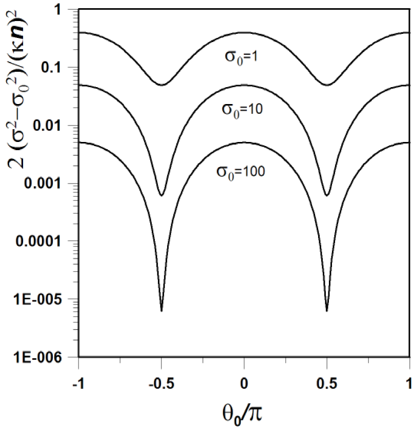
Figure 1: Using eq.(28) the function $2\frac{\sigma^{2}-{\sigma_{0}}^{2}}{(\kappa n)^{2}}$ is presented, in a log-scale, as a function of the initial angular position, $\theta_{0}/\pi$, for three values of $\sigma_{0}$: $1$, $10$ and $100$. The calculation corresponds to the primary resonance $p/q=1$.

From eq.(26) and eq.(23) the QKR group velocity is calculated

$$v_{g}=\frac{dM_{1}(n)}{dn}=\frac{1}{\hbar}\frac{dL(n)}{dn}=-\kappa\sin\theta_{0}\ e^{{-\frac{1}{8\sigma_{0}}}},$$ (29)

and we confirm that if $\theta_{0}=0$ then $v_{g}=0$, while if $\theta_{0}=\pm\pi/2$ then $v_{g}\simeq\pm\kappa$ for $\sigma_{0}>1$. This result is very interesting because it shows that if one chooses the value of $\theta_{0}$ appropriately in the initial condition of the QKR, one can get an average angular momentum pointing in a preset direction and increasing in time with a preset ratio $v_{g}$. In order to visualize the temporal evolution of the probability distribution in momentum space, we present the fig.2 obtained numerically using the original map eq.(7). There, the initial conditions $\theta_{0}=\pi/2$ in eq.(15) have been chosen so that the group velocity is negative, hence, the first moment moves to the left. The spreading of the wave function in the angular momentum space as time elapses can also be appreciated in the figure.

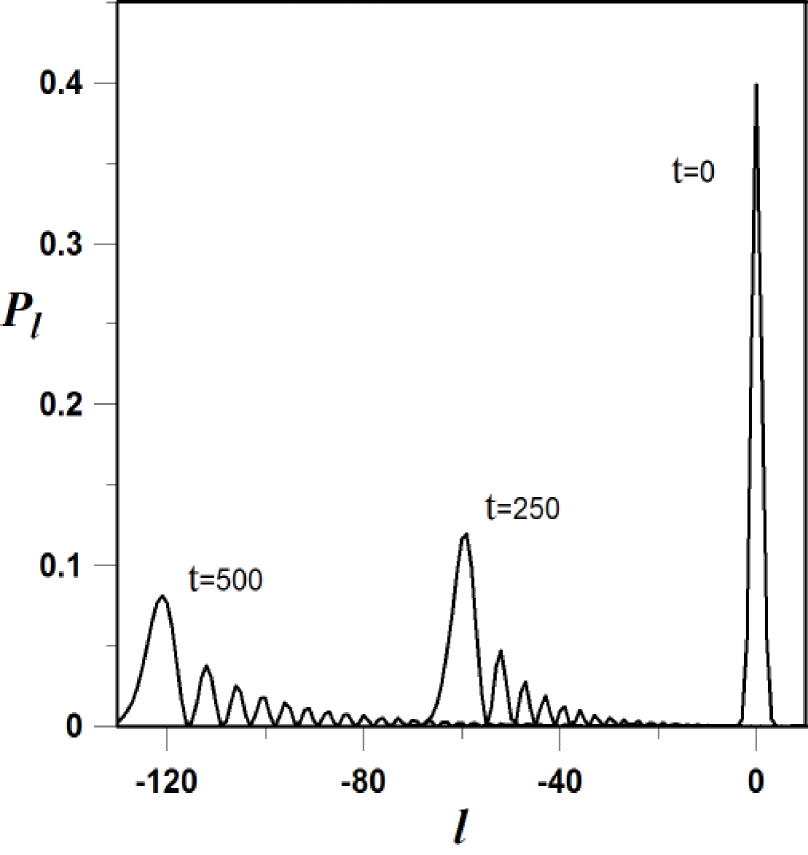
Figure 2: The probability distribution in momentum space as a function of the dimensionless angular momentum is presented for three times $t=0$, $t=250$ and $t=500$. The figure was obtained numerically from the map eq.(7) with $\kappa=0.25$ in the primary resonance $p/q=1$. The initial conditions have been given by eq.(15) with $\sigma_{0}=1$ and $\theta_{0}=\pi/2$.

Strictly, from eq.(28) and fig. 1 the values of $\theta_{0}$ and $\sigma_{0}$ cannot be chosen in order to produce $\sigma(n)=\sigma_{0}$ with $v_{g}\neq 0$. However, for $\theta_{0}=\pm\pi/2$ and $\sigma_{0}>1$ it is possible to produce a wavepacket with a constant shape that travels with constant velocity for a very long time. Additionally, in the asymptotic limit $\sigma_{0}\rightarrow\infty$, from eq.(29) we recover the expected equation eq.(13) that corresponds to the group velocity for a train of plane waves.

Therefore, we have demonstrated that the dispersion relation eq.(13) controls the velocity of the QKR wavepacket and the temporal evolution of its shape, see eqs.(26, 27).

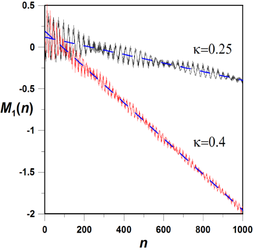
Figure 3: The first statistical moment as a function of the dimensionless time $n$ for two values of $\kappa=0.25$ and $0.4$. The dashed lines are lineal adjustment, the angular initial position is $\theta_{0}=\pi/2$ and $\sigma_{0}=1$. The calculation corresponds to the secondary resonance $p/q=1/3$.

5 Secondary resonances

We now study the incidence of extended initial distributions on the secondary resonances. In this case $p/q$ is not an integer and eq.(8) becomes too complicated to handle analytically, an exception being the antiresonance case $p/q=1/2$ Izrailev . Eq.(7) is no longer invariant under translations in the angular momentum. This invariance was fundamental for the previous analytical treatment. We therefore study numerically the influence of the extended initial conditions in the dynamics of the secondary resonances, using eq.(7) with $p/q=1/3$, and initial conditions given by eq.(15).

In fig. 3 we present the numerical calculation of the first statistical moment $M_{1}(n)$ as a function of time $n$, for two different values of $\kappa$ with $\theta_{0}=\pi/2$ and $\sigma_{0}=1$. This figure shows a complex oscillatory behavior where it is possible to define an average lineal behavior, shown by the blue dashed lines. The slopes of these straight lines define the corresponding group velocities for the secondary resonances. In fig. 4 we present the numerical calculation of the group velocity of the system as a function of the angular initial position. This figure shows a quasi sinusoidal dependence of $v_{g}$ with $\theta_{0}$, that reminds us of the behavior that was found for the primary resonances, eq.(29). However, if this behavior is compared to that of the previous case, now the oscillation frequency duplicates its value and its amplitude decreases by some orders of magnitude (note that this curve in fig. 4 is multiplied by $60$). Additionally, fig. 3 also shows that $v_{g}$ has a dependence with the strength parameter $\kappa$. We have obtained numerically this dependence and we synthesize the result in fig. 5. From this figure, it is clear that the simple proportionality obtained for the primary resonance, see eq.(26), has been lost.

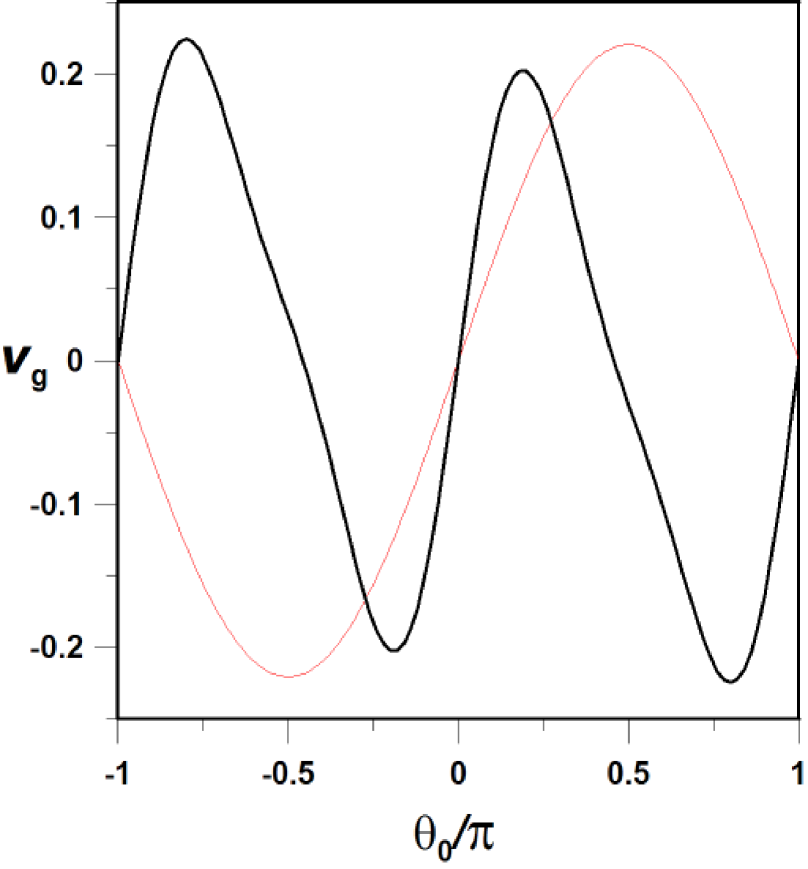
Figure 4: The dimensionless $v_{g}$ as a function of the initial angular position $\theta_{0}$ is presented. A thin red line is used for the primary resonance and a thick black line for the secondary resonance $p/q=1/3$. Both calculations have $\sigma_{0}=1$ and $\kappa=0.25$ but $v_{g}$ for the secondary resonance is multiplied by a factor of $60$.

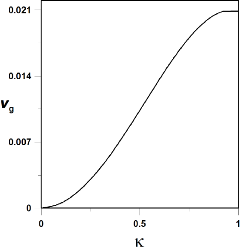
Figure 5: The dimensionless $v_{g}$ as a function of the strength parameter $\kappa$ for the secondary resonance $p/q=1/3$ with $\sigma_{0}=1$ and $\theta=\pi/4.$

6 Conclusion

In summary, through the use of the discrete Fourier transform in the study of the primary resonances of the QKR, it is straightforward to get an explicit dispersion relation. This dispersion relation is a powerful tool for predicting the QKR dynamics because it controls not only the velocity of the wavepacket, but also the evolution of its shape as time elapses. We show that the extension of the initial distribution can delay the characteristic time that the resonant evolution needs in order to exhibit its ballistic behavior. This result could explain the absence of the ballistic growth in some experimental realizations of the QKR. Additionally, from the analytical treatment we show the sinusoidal dependence between the energy and the initial average position of the system.

We also study, numerically, the influence of an extended initial distribution in the behavior of the secondary resonances of the QKR. We obtain a relation between the parameters of the extended initial condition and the dynamical average of the system. We show, as in the case of the primary resonances, that if one chooses the value of $\theta_{0}$ appropriately in the initial condition, one can get an average angular momentum pointing in a preset direction and increasing in time with a preset ratio $v_{g}$.

We acknowledge the support from PEDECIBA, CSIC, ANII and thank V. Micenmacher, E. Roldán and G. J. Valcárcel for their comments and stimulating discussions.

References

- (1) Casati G., Chirikov B. V., Izrailev F. M., Ford J., Lect. Notes Phys. 93, (1979) 334.
- (2) Schomerus H. Lutz E., Phys. Rev. Lett., 98 (2007) 260401.
- (3) Schomerus H. Lutz E., Phys. Rev. A 77, (2008) 062113.
- (4) Currivan J-A., Ullah A. Hoogerland M. D., Europhys. Lett. 85 (2009) 30005.
- (5) Sadgrove M., Hilliard A., Mullins T., Parkins S. Leonhardt R., Phys. Rev. E 70 (2004) 036217.
- (6) Saunders M., Halkyard P. L., Challis K. J. Gardiner S. A., Phys. Rev. A 76 (2007) 043415.
- (7) Halkyard P. L., Saunders M., and Gardiner S. A., Phys. Rev. A 78 (2008) 063401.
- (8) Chaudhury S., Smith A., Anderson B. E., Ghose S. Jessen P. S., Nature 461 (2009) 768.
- (9) Izrailev F. M. , Phys. Rep. 196 (1990) 299.
- (10) Goodman J. W. Introduction to Fourier optics, (Roberts and Company Publishers, 2005).
- (11) Patorski K., Progress in Optics (E. Wolf, XXVII, Elsevier Science, Amsterdam, 1989) 1-108.
- (12) Moore F. L., Robinson J. C., Bharucha C., Williams P. E. Raizen M. G., Phys. Rev. Lett. 73 (1994) 274. Robinson J. C. , Bharucha C., Moore F. L., Jahnke R., Georgakis G. A., Niu Q., Raizen M. G., Sundaram B., Phys. Rev. Lett. 74 (1995) 3963. Moore F. L., Robinson J. C., Bharucha C. F., Sundaram B. Raizen M. G., Phys. Rev. Lett. 75 (1995) 4598. Robinson J. C. , Bharucha C. F., Madison K. W., Moore F. L., Sundaram B., Wilkinson S. R. Raizen M. G., Phys. Rev. Lett. 76 (1996) 3304.
- (13) Bharucha C. F., Robinson J. C., Moore F. L., Sundaram B., Niu Q. Raizen M. G., Phys. Rev. E 60 (1999) 3881.
- (14) Oskay W. H., Steck D. A., Milner V., Klappauf B. G. Raizen M. G., Opt. Commun. 179 (2000) 137.
- (15) Kanem J. F., Maneshi S., Partlow M., Spanner M. Steinberg A. M., Phys. Rev. Lett. 98 (2007) 083004.
- (16) Valcárcel G. J., Roldán E. Romanelli A. , New J. Phys. 12 (2010) 123022.
- (17) Romanelli A. , Siri R. Micenmacher V. Phys. Rev. E 76 (2007) 037202.
- (18) Romanelli A., Phys. Rev. E 79 (2008) 056209.
- (19) Romanelli A., Phys. Rev. A 80 (2009) 022102.
- (20) Romanelli A., Sicardi Schifino A. C., Siri R., Abal G., Auyuanet A. Donangelo R., Physica A 338 (2004) 395.
- (21) Romanelli A., Auyuanet A., Siri R., Abal G. Donangelo R., Physica A 352 (2005) 409.
- (22) Romanelli A., Auyuanet A., Siri R. Micenmacher V., Phys. Lett. A 365 (2007) 200.
- (23) Romanelli A., Phys. Lett. A 80 (2009) 042332.
- (24) Gradshteyn I. S. Ryzhik I. M. Table of Integrals Series and Products. (Academic Press, New York 1994), 987.