Water in low-mass star-forming regions with Herschel (WISH-LM)

Herschel-HIFI observations of water in the low-mass star-forming object L1448-MM, known for its prominent outflow, are presented, as obtained within the ‘Water in star-forming regions with Herschel’ (WISH) key programme. Six H${}_{2}^{16}$O lines are targeted and detected ($E_{\rm up}$/$k_{\rm B}$$\sim$50–250 K), as is CO $J$= 10–9 ($E_{\rm up}/k_{\rm B}$$\sim$305 K), and tentatively H${}_{2}^{18}$O 1₁₀–1₀₁ at 548 GHz. All lines show strong emission in the “bullets” at $|\varv|$$>$50 km s^-1 from the source velocity, in addition to a broad, central component and narrow absorption. The bullets are seen much more prominently in H₂O than in CO with respect to the central component, and show little variation with excitation in H₂O profile shape. Excitation conditions in the bullets derived from CO lines imply a temperature $>$150 K and density $>$10⁵ cm^-3, similar to that of the broad component. The H₂O/CO abundance ratio is similar in the “bullets” and the broad component, $\sim$0.05–1.0, in spite of their different origins in the molecular jet and the interaction between the outflow and the envelope. The high H₂O abundance indicates that the bullets are H₂ rich. The H₂O cooling in the “bullets” and the broad component is similar and higher than the CO cooling in the same components. These data illustrate the power of Herschel-HIFI to disentangle different dynamical components in low-mass star-forming objects and determine their excitation and chemical conditions.

1 Introduction

Low-mass star formation is accompanied by the launch of powerful jets that drive strong shocks into the parental material (e.g., Arce et al. 2007), both in the form of shell shocks that interact with the molecular envelope, and in the form of the jet itself (e.g., Hirano et al. 2010). The jets are generally not uniform, but consist of small condensations (“bullets”), that can be attributed to internal working surfaces caused by episodic ejection of material from the protostar (Santiago-García et al. 2009). The bullets are chemically rich, in particular in oxygen-bearing species (Tafalla et al. 2010), and should therefore display high abundances of water. H₂O is one of the best shock tracers because the abundance can increase by orders of magnitude up to $\lesssim$10^-4 through sputtering of grain mantles and formation in the gas phase at high temperatures (Flower & Pineau des Forêts 2010). Also, due to the large velocity gradients in shocks, emission is effectively optically thinner than in a quiescent object (Franklin et al. 2008).

H₂O has previously been observed in outflowing gas from young stellar objects (YSOs) using, e.g., Odin, SWAS, and ISO. The Heterodyne Instrument for the Far-Infrared (HIFI) on Herschel opens up spectrally resolved, high angular resolution observations of both H₂O and high-$J$ CO in low-mass protostars (e.g., Lefloch et al. 2010, Yıldız et al. 2010, Kristensen et al. 2010). The latter paper presents H₂O observations of the low-mass star-forming region NGC1333. The H₂O line profiles are complex, consisting of three velocity components characterised by their width. The broadest component ($\Delta\varv$$>$20 km s^-1) originates in the interaction between the outflow and the envelope; the medium-broad component (5$<$$\Delta\varv$$<$20 km s^-1) arises where the jet impacts on the inner, dense envelope; a narrow absorption component ($\Delta\varv$$<$5 km s^-1) is attributed to the cold outer envelope. These initial HIFI results show that H₂O is one of the best dynamics tracers in YSOs, and confirm that the H₂O/CO abundance increases with velocity to $\sim$1. To date, H₂O has not been uniquely identified in the bullets, and its abundance with respect to other jet species is unknown. Moreover, the different nature of the shocks could lead to different H₂O abundances.

L1448-MM is a low-mass, Class 0 protostar located in Perseus ($L$=11.6 $L_{\odot}$, $M_{\rm env}$=1.9 $M_{\odot}$, $d$ = 235 pc; van Dishoeck et al. 2011). This object is the prototype of the class of sources showing bullet emission in CO (Bachiller et al. 1990), with red- and blue-shifted emission peaks at $\sim$ $\pm$50 km s^-1 with respect to $\varv_{\rm LSR}$ = $+$5.2 km s^-1. The bullets are clearly visible in other shock tracers such as SiO (e.g. Nisini et al. 2007), and have been imaged at high spatial resolution using interferometers (e.g., Guilloteau et al. 1992, Hirano et al. 2010). Our observations of H₂O within the framework of the ‘Water in star-forming regions with Herschel’ (WISH; van Dishoeck et al. 2011) key programme further explore the chemical and excitation conditions of shocked gas in low-mass star-forming regions.

2 Observations and results

The central position of L1448-MM (03^h25^m38$\aas@@fstack{s}$9; $+$30°44′05$\aas@@fstack{\prime\prime}$4; J2000) was observed with HIFI on Herschel (de Graauw et al. 2010, Pilbratt et al. 2010) in seven different settings covering six H${}_{2}^{16}$O, two H${}_{2}^{18}$O and one CO transition ($E_{\rm u}/k_{\rm B}\approx 50-300$ K; Table 5 available online). Data were obtained using the dual beam-switch mode with a nod of 3′, except for the ground-state ortho-H₂O line at 557 GHz, where a position switch to ($+$10′; $+$5′) was used. The diffraction-limited beam size ranges from 19″ to 39″ (4500–9500 AU). Data were reduced using HIPE ver. 4.0. The calibration uncertainty is taken to be 10% for lines observed in Bands 1, 2, and 5 while it is 30% in Band 4. The pointing accuracy is $\sim$2″. A main-beam efficiency of 0.65–0.75 is adopted (Table 5). Subsequent analysis of the data is performed in CLASS including subtraction of linear baselines. H- and V-polarizations are co-added after inspection; no significant differences are found between the two data sets. ¹²CO 3–2 and ¹³CO 3–2 were observed with the James Clerk Maxwell Telescope (JCMT). CO 2–1 was observed at the IRAM 30m (Tafalla et al. 2010), and CO 4–3 at the JCMT (Nisini et al. 2000).

All targeted lines are detected, except H${}_{2}^{18}$O 1₁₁–0₀₀, observed with the main isotopologue (Fig. 1). This figure strikingly demonstrates that the bullets are much more prominent in H₂O than in CO relative to the central component. Also, the H₂O profiles are very different from those seen in NGC 1333 (Kristensen et al. 2010). Each line consists of multiple components: two Gaussian peaks at velocities of $\sim$ $\pm$50 km s^-1 with respect to $\varv_{\rm source}$; a broad ($\sim$50 km s^-1) component centered close to $\varv_{\rm source}$; and a narrow ($\sim$5 km s^-1) component seen in absorption at $\varv_{\rm source}$. The extremely high-$\varv$ emission (henceforth EHV-B and EHV-R) is detected in all lines, although the detection in the H${}_{2}^{18}$O 1₁₀–1₀₁ line is tentative (2$\sigma$; 0.13 K km s^-1). The emission components are well reproduced by Gaussians and fitted to obtain the integrated intensity (Table 2). The H₂O line profiles vary little with excitation. The shape of the EHV component in the CO profiles resembles that of H₂O (Fig. 4, appendix), whereas the the broad component is much weaker in CO. The CO lines also contain a narrower component ($\sim$10 km s^-1) not seen in H₂O.

To compare observations done with different beam sizes, all observations are scaled to a common beam of 22″, the beam at 988 GHz. The scaling follows the recipe outlined in Appendix B of Tafalla et al. (2010), where a linear scaling with beam size is found to be appropriate for the EHV components and a power-law scaling with index 0.75 for the broad component. It is only significant for the 557 GHz lines due to the larger beam (39″).

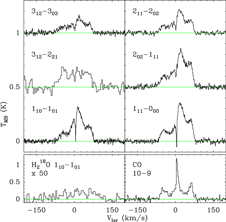
Figure 1: Continuum-subtracted HIFI H₂O, H${}_{2}^{18}$O and CO spectra obtained at the central position of L1448-MM ($\varv_{\rm source}$ = 5.2 km s^-1).

Table 1: H₂O, H${}_{2}^{18}$O and CO emission in each velocity component.

		EHV-B	EHV-R	Broad
Transition	rms	$\int T_{\rm MB}\leavevmode\nobreak\ {\rm d}\varv$	$\int T_{\rm MB}\leavevmode\nobreak\ {\rm d}\varv$	$\int T_{\rm MB}\leavevmode\nobreak\ {\rm d}\varv$
	(mK)	(K km s-1)	(K km s-1)	(K km s-1)
H2O 110–101	9	2.54	3.00	14.4
111–000	11	3.98	4.00	14.8
202–111	14	4.01	3.86	17.6
211–202	14	2.47	2.53	9.9
312–303	13	2.34	1.14	7.8
312–221	66	6.22	3.32	7.9
H${}_{2}^{18}$O 110–101	3	0.13	0.11	0.23
111–000	11	$<$0.25	$<$0.19	$<$0.28
CO 2–1	51	2.79	4.12	38.5
3–2	39	4.82	6.58	44.9
4–3	160	11.9	15.1	74.6
10–9	66	7.30	8.42	17.8
FWHM (km s-1)		38.4$\pm$3.2	22.4$\pm$3.0	47.6$\pm$4.5
$\varv_{\rm LSR}$ (km s-1)		$-$43.4$\pm$1.3	59.3$\pm$1.8	16.8$\pm$2.2

The tentative detection of the H${}_{2}^{18}$O 1₁₀–1₀₁ (548 GHz) line is used to constrain the optical depth, $\tau$, of the main isotopologue, assuming that the line itself is optically thin and that [¹⁶O]/[¹⁸O]=550. The optical depth, $\tau$, is $\sim$25 in each EHV component and 9 in the broad component implying that emission from H${}_{2}^{16}$O 1₁₀–1₀₁ is optically thick. The 3$\sigma$ upper limit on the H${}_{2}^{18}$O 1₁₁–0₀₀ line implies $\tau$$\lesssim$10 and $\lesssim$30 in H${}_{2}^{16}$O for the broad and EHV components, respectively. ¹³CO 3–2 emission is not detected in any of the components. The ¹²CO 3–2 optical depth is $\lesssim$2 and $\lesssim$0.3 in the EHV and broad components, respectively, implying that the CO emission is optically thin.

The integrated intensities of each of the EHV and broad components are used to construct Boltzmann diagrams, where the column density of each upper level in the optically thin limit ($N_{\rm up}^{*}$) per sub-level is plotted versus $E_{\rm up}$ (Fig. 2). In the diagrams, $N_{\rm up}^{*}$ for the H₂O ground-state transitions is lower than expected, confirming that the true $N_{\rm up}$ is higher and that the lines are optically thick. Excluding these two lines from further analysis, the resulting rotational temperature is remarkably similar for all three components ($\sim$45–60 K), while the beam-averaged column density of the broad component is $\sim$5 times higher than that of the EHV components ($\sim$10 and 2$\times$10¹³ cm^-2, respectively; Table 2). Rotational diagrams are also made for CO and results are given in Table 2. $T_{\rm rot}$ is significantly higher, 150 K in the EHV components and 80 K in the broad. The column density is also higher, $\sim$10¹⁶ cm^-2, and the inferred H₂O/CO ratio is $\sim$0.002.

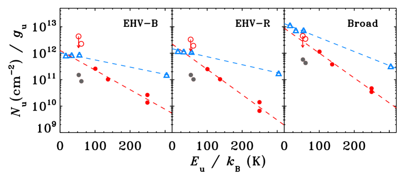
Figure 2: Rotational diagrams of the EHV and broad components for H₂O (red circles) and CO (blue triangles). CO has been shifted downwards by a factor of 100. The ground-state transitions (grey) are excluded from the fit (dashed lines). H${}_{2}^{18}$O intensities $\times$550 are shown as open circles.

Table 2: Rotational-diagram results for each velocity component.

	H2O			CO
Component	$T_{\rm rot}$	$N$		$T_{\rm rot}$	$N$
	(K)	(1013 cm-2)		(K)	(1015 cm-2)
EHV-B	58$\pm$4	1.9$\pm$0.4		160$\pm$18	26.0$\pm$0.7
EHV-R	45$\pm$3	2.4$\pm$0.5		144$\pm$14	27.6$\pm$0.8
Broad	46$\pm$2	9.5$\pm$2.1		82$\pm$4	38.6$\pm$3.9

3 Discussion

3.1 Excitation conditions

To determine the physical parameters, a small grid of RADEX slab models was run (van der Tak et al. 2007). This grid is first used to determine CO excitation conditions by fitting $T_{\rm rot}$ (see Fig. 5 in the on-line appendix). To reproduce $T_{\rm rot}$$\sim$150 K as observed in the EHV components, a kinetic temperature of 150 K and density greater than $\sim$10⁶ cm^-3 is required. Alternatively, a kinetic temperature of $\sim$500 K and density of $\sim$10⁵ cm^-3 can also reproduce the observed CO rotational temperature. In the following, both sets of values, ($T$, $n$) = (150 K, 10⁶ cm^-3; model 1), and (500 K, 10⁵ cm^-3; model 2), will be examined to constrain the H₂O excitation. Similar values are needed to reproduce the lower CO rotational temperature of the broad component, $T_{\rm rot}$$\sim$80 K, ($T$, $n$) = (100 K, 10⁶ cm^-3) and (500 K, 5$\times$10⁴ cm^-3). The latter solution is excluded, however, because the envelope density within the 20$\arcsec$ beam is always $>$ 4$\times$10⁵ cm^-3. Independent analysis of outflow emission (Nisini et al. 1999; 2000) indicate that H₂O is excited in a hotter, denser medium than CO, and for this reason a model with ($T$, $n$) = (500 K, 10⁶ cm^-3; model 3), is included in the analysis.

To constrain the H₂O excitation, the same physical conditions as determined for CO are taken as fixed and line widths of 40 and 20 km s^-1 for the EHV-B and EHV-R components, respectively, and 50 km s^-1 for the broad component are adopted. C-type shock models show that CO and H₂O cooling takes place at the same location in a shock (Flower & Pineau des Forêts 2010), thus validating this assumption. The H₂O o/p ratio is assumed to be 3, and the only variable in the RADEX modelling is the total H₂O column density. To constrain this, the ratio of the higher-excited H${}_{2}^{16}$O lines is taken with respect to the 2₀₂–1₁₁ line, and the calculated emission in this line is constrained to be greater than the observed value. The same is done for the H${}_{2}^{18}$O tentative detection and upper limit. A $\chi^{2}$ analysis is used to determine the best-fit value of the H₂O column density. Once the column density is determined, the predicted intensity is compared to the observed intensity of the 2₀₂–1₁₁ line, and from this the filling factor is determined. The predicted column density is re-scaled to the average column density in the beam, and compared to $N$(CO) to determine the H₂O/CO abundance ratio.

The best-fit results are listed in Table 3. $N$(H₂O) is found to be $\sim$10¹⁶–10¹⁸ cm^-2 for all components and all three models, implying a beam filling factor of $\lesssim$0.01–0.1. This leads to an average H₂O/CO abundance ratio of $\sim$0.05–1.0 in all of the components; the range is caused by the excitation model rather than differences between the physical components. This result is very different from the rotational-diagram analysis above, where the abundance ratio is a factor of $>$100 lower. The difference arises because H₂O is not thermalised and optically thick, as opposed to CO, and thus non-LTE, radiative-transfer models are needed to treat the excitation properly. Figure 3 shows the H₂O/CO ratio as function of $N$(H₂O) demonstrating that only model 3 produces abundance ratios $\lesssim$0.1.

The RADEX models that match the H₂O line emission best predict that the filling factor for the EHV component is very small, $<$0.01. Such low values agree with high spatial-resolution observations showing this component to be confined to the molecular jet and consisting of several sub-arcsec knots (e.g., Hirano et al. 2010). The model furthermore predicts that the ground-state transitions have optical depths in excess of 100 (Fig. 6, online appendix), and that the two H${}_{2}^{18}$O transitions and the higher-excited H${}_{2}^{16}$O transitions are also optically thick ($\tau$$\sim$3–4). Thus, the optical depth derived from the line ratios can only be considered a relative optical depth between the two transitions. If the H${}_{2}^{18}$O 1₁₀–1₀₁ transition is assumed to be optically thin, a typical H₂O column density of a few times 10¹⁵ cm^-2 is required. However, models with this column density predict that the intensity of the 2₀₂–1₁₁ line is close to that observed, or lower in the case of the broad component, implying filling factors of unity inconsistent with the bullet nature. The CO emission remains optically thin ($\tau$$<$1) for all three models even with the small filling factors derived for H₂O, consistent with the non-detection of ¹³CO 3–2.

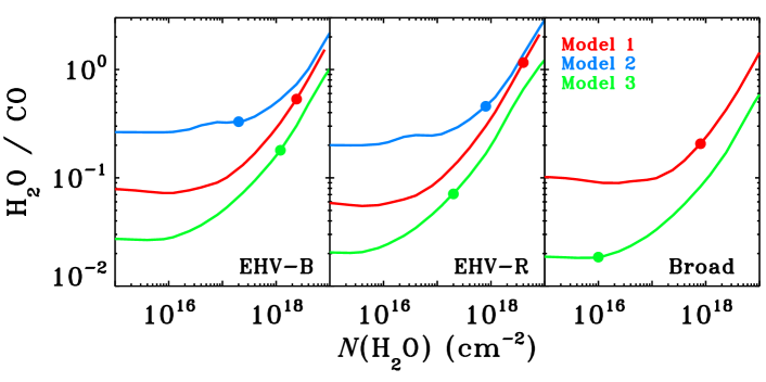
Figure 3: H₂O/CO ratio as a function of H₂O column density for the three different models 1, 2 and 3. The best-fit results are marked with points.

Table 3: Modelled H₂O line emission and inferred parameters.

	$N$(H2O)	$\chi^{2}_{\rm red}$	$\int$ $T$(202–111) d$\varv$	Filling factor	H2O/CO
	(1018 cm-2)		(K km s-1)	($\times$10-3)
Model 1:
EHV-B	2.4	0.4	3000	1.3	0.5
EHB-R	0.2	0.4	2870	4.4	0.1
Broad	1.2	1.5	2070	8.3	0.3
Model 2:
EHV-B	4.0	0.9	2650	1.5	1.0
EHB-R	0.8	0.4	2890	4.3	0.5
Model 3:
EHV-B	0.80	0.5	3800	1.1	0.1
EHB-R	0.08	0.9	3890	4.3	0.05
Broad	0.01	0.2	3290	65.0	0.02

3.2 Physical origin

3.2.1 EHV versus broad components

Following the interpretation of the EHV emission in IRAS04191 (Santiago-García et al. 2009) it seems likely that the knots are internal working surfaces (IWS) along the jet that appear as strongly beam-diluted emission in single-dish observations. Regardless of the precise shock details, the high abundance of H₂O in the bullets implies a high H₂ fraction, since otherwise reactions with atomic H drive H₂O back to OH and atomic O.

The timescale for H₂O to be produced in gas as a function of temperature has been determined by Bergin et al. (1998) for $n$=10⁵ cm^-3. For $T$=500 K, the timescale is $\sim$100 years, which may be compared to the maximum dynamical time for a bullet with velocity 50 km s^-1 to leave a beam with radius 11″, 240 years. Thus, it is possible to reform H₂O from atomic gas over the timescales associated with the bullets. In the lower-$T$ scenario, H₂O will not form in the quantities observed here implying that the temperature is high in the bullets or that H₂O is not formed in the gas phase.

The gas-phase production of H₂O is in agreement with models of continuous spherical wind models of Glassgold et al. (1991), where the formation takes place from a dust-free atomic gas in sufficient quantities if the mass-loss rate exceeds 10^-5 $M_{\odot}$ yr^-1, which is to be compared to the time-averaged mass-loss rate in the jet of $\sim$10^-6 $M_{\odot}$ yr^-1 (Hirano et al. 2010). The mass loss rate traced directly by the bullets is episodic (and thus higher than the time-averaged value) and the wind is not spherical, i.e., it is plausible that the H₂O abundance is consistent with production in the IWS from atomic gas. To resolve the issue of the origin of the molecules and to break the degeneracy between the different models, it is necessary to obtain velocity-resolved data of chemically related species, such as O and OH. Furthermore, measuring the H/H₂ ratio would test the models.

The broad component, centered near $\varv_{\rm LSR}$, is now observed in H₂O emission in a number of low-mass sources (Kristensen et al. 2010, in prep.). It is interpreted as arising in the interaction between the outflow and envelope, and is seen so prominently in H₂O emission (as opposed to, e.g., CO) due to the high production rate of H₂O at this location. H₂O is formed through both a series of neutral-neutral reactions pushing atomic oxygen into water, and through sputtering of icy grain mantles. Quantifying the contributions from the different mechanisms require observations of other grain-surface products, e.g., CH₃OH, and velocity-resolved observations of the intermediate gas-phase products O and OH. Tafalla et al. (2010) detect CH₃OH emission in both the EHV and broad components (but at an outflow position) indicating that a significant fraction of H₂O is sputtered from grains.

3.2.2 Cooling

The observed cooling rate in the three components is found by summing up the observed line emission (Table 4). For the EHV components, the H₂O cooling rate is $\sim$ 3.5$\times$10^-4 $L_{\odot}$, while it is $\sim$1.3$\times$10^-3 $L_{\odot}$ for the broad. Extrapolating the cooling to include all lines with wavelengths greater than 60 $\mu$m gives a total H₂O luminosity of 2–4$\times$10^-2 $L_{\odot}$ depending on which model is used (Table 4), i.e., the cooling by the lines observed with HIFI amounts to $\sim$10%. The cooling is nearly the same for all three components demonstrating the power of spectrally resolving line profiles. This number may be compared to 4.5$\times$10^-2 $L_{\odot}$ as was found for H₂O by ISO-LWS in an 80″ beam (Nisini et al. 2000), which applies to the sum of the components.

The observed CO cooling rate is somewhat higher, $\sim$2$\times$10^-3 and 6.0$\times$10^-3 $L_{\odot}$, respectively. The CO cooling rate for the three components is extrapolated using the rotational diagrams to a total of 4.0$\times$10^-3 $L_{\odot}$, lower than the H₂O cooling. The EHV components contribute $\sim$50% to the CO cooling. ISO-LWS observed a total CO cooling rate of 3.0$\times$10^-2 $L_{\odot}$ (Nisini et al. 2000), but in a much larger beam encompassing the extended outflow emission and other physical components (van Kempen et al. 2010).

Table 4: H₂O and CO cooling rates in 10^-3 $L_{\odot}$.

		EHV-B	EHV-R	Broad	Total
H2O:	Observed emission	00.4	0.3	01.1	01.8
	Model 1 extrapol.	11.0	4.8	26.6	42.4
	Model 2 extrapol.	10.7	6.4	…	17.1
	Model 3 extrapol.	15.1	6.5	11.7	33.3
CO:	Observed emission	00.2	0.2	00.4	00.8
	$T_{\rm ex}$ extrapol.	01.1	1.1	01.8	04.0

4 Conclusions

H₂O emission readily traces the EHV gas that has previously only been seen in very deep integrations of other species, such as CO. The EHV components are attributed to shocks in the molecular jet, while the underlying broad component, now seen in several low-mass YSOs, is associated with the interaction of the outflow and the envelope on larger scales. Thus, HIFI and H₂O together are ideal for revealing the dynamical components of low-mass star-forming regions. Both components are H₂ rich, since otherwise the H₂O abundance would be lower. The two distinct components appear remarkably similar in terms of excitation and chemical conditions in spite of their different chemistries. They have equal contributions from H₂O and CO cooling with H₂O being the dominant coolant of the two. High spectral-resolution observations are a prerequisite for interpreting spectrally unresolved PACS data of the same source.

Appendix A Gauss fit of data

The data are fitted by Gaussians, with the exception of the narrow absorption component. Figure 4 shows the example of the H₂O 1₁₁–0₀₀ line, with the residual plotted below. Furthermore, Fig. 4 shows the CO 3–2 line scaled and overplotted on the H₂O 1₁₁–0₀₀ line, highlighting the similar line profile in the EHV components.

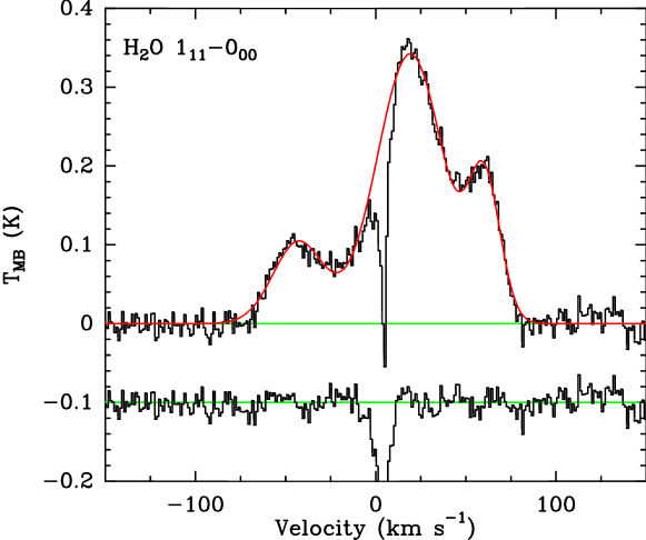
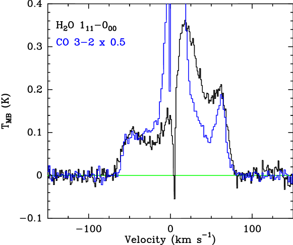
Figure 4: (Top:) Gauss fit of the H₂O 1₁₁–0₀₀ line (red) with the residual shown below (offset at $-$0.1 K). The central absorption feature is not fitted. (Bottom:) CO 3–2 scaled to the peak intensity of H₂O in the bullets and overplotted on the H₂O 1₁₁–0₀₀ line.

2

Table 5: H₂O, H${}_{2}^{18}$O and CO emission in each velocity component at the source position.

		EHV-B					EHV-R					Broad
Transition	rms	$T_{\rm MB}^{\rm peak}$	$\int T_{\rm MB}\leavevmode\nobreak\ {\rm d}\varv$	$FWHM$	$\varv_{\rm LSR}$		$T_{\rm MB}^{\rm peak}$	$\int T_{\rm MB}\leavevmode\nobreak\ {\rm d}\varv$	$FWHM$	$\varv_{\rm LSR}$		$T_{\rm MB}^{\rm peak}$	$\int T_{\rm MB}\leavevmode\nobreak\ {\rm d}\varv$	$FWHM$	$\varv_{\rm LSR}$
	(mK)	(mK)	(K km s-1)	(km s-1)	(km s-1)		(mK)	(K km s-1)	(km s-1)	(km s-1)		(mK)	(K km s-1)	(km s-1)	(km s-1)
H2O 110–101	9	74	2.54	32.3	$-$44.2		122	3.00	23.0	60.1		294	14.40	46.0	14.0
111–000	11	101	3.98	37.1	$-$41.1		176	4.00	21.3	60.1		337	14.76	41.2	20.1
202–111	14	93	4.01	40.3	$-$43.7		175	3.86	20.7	59.8		328	17.59	50.4	18.0
211–202	14	65	2.47	35.9	$-$44.2		109	2.53	21.9	60.0		207	9.91	44.9	15.4
312–303	13	50	2.34	44.0	$-$45.4		65	1.14	16.5	60.7		124	7.76	54.5	16.3
312–221	66	147	6.22	39.7	$-$43.1		111	3.32	28.1	55.4		139	7.94	53.4	14.8
H${}_{2}^{18}$O 110–101	3	4	0.13	…	…		5	0.11	…	…		5	0.23	…	…
111–000	11	…	$<$0.25	…	…		…	$<$0.19	…	…		…	$<$0.28	…	…
CO 2–1	51	184	2.79	14.2	$-$51.6		280	4.12	13.8	60.3		498	38.53	72.8	0.8
3–2	39	216	4.82	21.0	$-$48.2		467	6.58	13.2	61.9		657	44.85	64.1	8.0
4–3	160	467	11.9	24.0	$-$45.1		808	15.1	17.5	65.7		1023	74.61	68.5	19.0
10–9	66	269	7.30	25.5	$-$47.2		426	8.42	18.6	61.3		323	17.77	51.6	10.1

3

Table 6: H₂O, H${}_{2}^{18}$O and CO transitions observed with Herschel-HIFI.

Transition	$\nu$	$\lambda$	$E_{\rm u}/k_{\rm B}$	$A$	Beam	$t_{\rm int}$	$\eta_{\rm MB}$
	(GHz)	($\mu$m)	(K)	($10^{-3}$ s-1)	(′′)	(min.)
H2O    110–101	1556.94	538.29	161.0	13.46	39	13.0	0.74
111–000	1113.34	269.27	153.4	18.42	19	43.5	0.75
202–111	1987.93	303.46	100.8	15.84	22	23.3	0.73
211–202	1752.03	398.64	136.9	17.06	29	18.4	0.74
312–303	1097.37	273.19	249.4	16.48	20	32.4	0.75
312–221	1153.13	259.98	249.4	12.63	19	13.0	0.65
H${}_{2}^{18}$O    110–101	1547.68	547.39	160.5	13.59	39	64.3	0.74
111–000	1101.70	272.12	152.9	21.27	20	43.5	0.75
CO            10–9	1151.99	260.24	304.1	0.10	19	13.0	0.65

Appendix B RADEX results

The non-LTE, escape-probability code RADEX was used to create rotational diagrams for H₂O and CO in the optically thin limit. Collisional rate coefficients are from Faure et al. (2007) and Yang et al. (2010), respectively. The same transitions as observed were then used to calculate the rotational temperature as function of $T_{\rm kin}$ and $n_{\rm H}$. The results are shown in Fig. 5.

RADEX was also used to calculate the optical depth, $\tau$ of the H${}_{2}^{16}$O 1₁₀–1₀₁ line at 557 GHz. Results are shown in Fig. 6, where also the beam-filling factor is shown as a function of H₂O column density for the three different models.

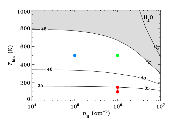
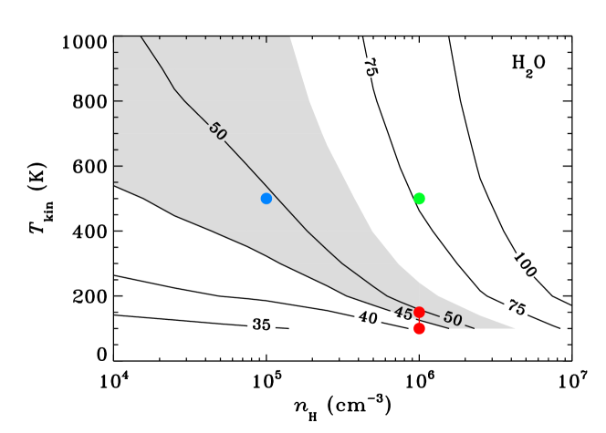
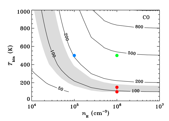
Figure 5: $T_{\rm rot}$ of optically thin H₂O emission (top), optically thick H₂O emission ($N$=10¹⁷ cm^-2; middle) and optically thin CO emission (bottom) determined from RADEX simulations. $T_{\rm rot}$ is calculated from the same transitions as in Sect. 2, i.e., excluding the ground-state transitions. The gray area indicates the observed values of $T_{\rm rot}$. The points indicate the different physical conditions examined; model 1 (red) has ($T$, $n$) = (150 K, 10⁶ cm^-3) for the EHV components and (100 K, 10⁶ cm^-3) for the broad component. Model 2 (blue) has ($T$, $n$) = (500 K, 10⁵ cm^-3) for the EHV components, respectively. Model 3 (green) has ($T$, $n$) = (500 K, 10⁶ cm^-3) for all components.

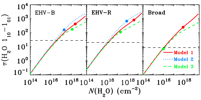
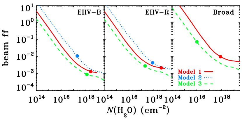
Figure 6: (Top:) $\tau$ of the H${}_{2}^{16}$O 1₁₀–1₀₁ line. The black dashed line corresponds to the observed value in each of the three velocity components as specified in Sect. 2. (Bottom:) Beam-filling factor for the three different components and three different models as a function of total H₂O column density. Best-fit results are marked with points in both plots.

References

- Arce et al. (2007) Arce, H. G., Shepherd, D., Gueth, F., et al. 2007, in Protostars and Planets V, ed. B. Reipurth, D. Jewitt, & K. Keil, 245–260
- Bachiller et al. (1990) Bachiller, R., Martin-Pintado, J., Tafalla, M., Cernicharo, J., & Lazareff, B. 1990, A&A, 231, 174
- Bergin et al. (1998) Bergin, E. A., Neufeld, D. A., & Melnick, G. J. 1998, ApJ, 499, 777
- de Graauw et al. (2010) de Graauw, T., Helmich, F. P., Phillips, T. G., et al. 2010, A&A, 518, L6
- Faure et al. (2007) Faure, A., Crimier, N., Ceccarelli, C., et al. 2007, A&A, 472, 1029
- Flower & Pineau des Forêts (2010) Flower, D. R. & Pineau des Forêts, G. 2010, MNRAS, 406, 1745
- Franklin et al. (2008) Franklin, J., Snell, R. L., Kaufman, M. J., et al. 2008, ApJ, 674, 1015
- Glassgold et al. (1991) Glassgold, A. E., Mamon, G. A., & Huggins, P. J. 1991, ApJ, 373, 254
- Guilloteau et al. (1992) Guilloteau, S., Bachiller, R., Fuente, A., & Lucas, R. 1992, A&A, 265, L49
- Hirano et al. (2010) Hirano, N., Ho, P. P. T., Liu, S., et al. 2010, ApJ, 717, 58
- Kristensen et al. (2010) Kristensen, L. E., Visser, R., van Dishoeck, E. F., et al. 2010, A&A, 521, L30
- Lefloch et al. (2010) Lefloch, B., Cabrit, S., Codella, C., et al. 2010, A&A, 518, L113
- Nisini et al. (1999) Nisini, B., Benedettini, M., Giannini, T., et al. 1999, A&A, 350, 529
- Nisini et al. (2000) Nisini, B., Benedettini, M., Giannini, T., et al. 2000, A&A, 360, 297
- Nisini et al. (2007) Nisini, B., Codella, C., Giannini, T., et al. 2007, A&A, 462, 163
- Pickett et al. (1998) Pickett, H. M., Poynter, I. R. L., Cohen, E. A., et al. 1998, Journal of Quantitative Spectroscopy and Radiative Transfer, 60, 883
- Pilbratt et al. (2010) Pilbratt, G. L., Riedinger, J. R., Passvogel, T., et al. 2010, A&A, 518, L1
- Santiago-García et al. (2009) Santiago-García, J., Tafalla, M., Johnstone, D., & Bachiller, R. 2009, A&A, 495, 169
- Tafalla et al. (2010) Tafalla, M., Santiago-García, J., Hacar, A., & Bachiller, R. 2010, A&A, 522, A91
- van der Tak et al. (2007) van der Tak, F. F. S., Black, J. H., Schöier, F. L., Jansen, D. J., & van Dishoeck, E. F. 2007, A&A, 468, 627
- van Dishoeck et al. (2011) van Dishoeck, E. F., Kristensen, L. E., Benz, A. O., et al. 2011, PASP, 123, 138
- van Kempen et al. (2010) van Kempen, T., Kristensen, L., Herczeg, G., et al. 2010, A&A, 518, L121
- Yang et al. (2010) Yang, B., Stancil, P. C., Balakrishnan, N., & Forrey, R. C. 2010, ApJ, 718, 1062
- Yıldız et al. (2010) Yıldız, U. A., van Dishoeck, E. F., Kristensen, L. E., et al. 2010, A&A, 521, L40
Acknowledgements.
HIFI has been designed and built by a consortium of institutes and university departments from across Europe, Canada and the US under the leadership of SRON Netherlands Institute for Space Research, Groningen, The Netherlands with major contributions from Germany, France and the US. Consortium members are: Canada: CSA, U.Waterloo; France: CESR, LAB, LERMA, IRAM; Germany: KOSMA, MPIfR, MPS; Ireland, NUI Maynooth; Italy: ASI, IFSI-INAF, Arcetri-INAF; Netherlands: SRON, TUD; Poland: CAMK, CBK; Spain: Observatorio Astronomico Nacional (IGN), Centro de Astrobiolog\ ́ia (CSIC-INTA); Sweden: Chalmers University of Technology - MC2, RSS & GARD, Onsala Space Observatory, Swedish National Space Board, Stockholm University - Stockholm Observatory; Switzerland: ETH Zürich, FHNW; USA: Caltech, JPL, NHSC. Astrochemistry in Leiden is supported by NOVA, by a Spinoza grant and grant 614.001.008 from NWO, and by EU FP7 grant 238258. The WISH team is thanked for stimulating discussions.Appendix A Gauss fit of data