Comparison of Signals from Gravitational Wave Detectors with Instantaneous Time-Frequency Maps

Abstract

Gravitational wave astronomy relies on the use of multiple detectors, so that coincident detections may distinguish real signals from instrumental artifacts, and also so that relative timing of signals can provide the sky position of sources. We show that the comparison of instantaneous time-frequency and time-amplitude maps provided by the Hilbert-Huang Transform (HHT) can be used effectively for relative signal timing of common signals, to discriminate between the case of identical coincident signals and random noise coincidences, and to provide a classification of signals based on their time-frequency trajectories. The comparison is done with a $\chi^{2}$ goodness-of-fit method which includes contributions from both the instantaneous amplitude and frequency components of the HHT to match two signals in the time domain. This approach naturally allows the analysis of waveforms with strong frequency modulation.

1 Introduction

The Hilbert-Huang Transform (HHT) [1] is a novel data analysis technique used to detect and characterize physical oscillatory modes in time series data. It is adaptive and data driven, making it directly applicable to data containing transient signals and non-stationary noise [2]. It consists of the empirical mode decomposition (EMD), followed by the Hilbert Spectral Analysis (HSA). The EMD process consists of forming an envelope about the extrema of the data by cubic spline fitting, and then subtracting the average of the envelope from the data. The extrema of remainder are then fitted, and the process is repeated as many times as necessary to obtain a waveform that is symmetric about zero mean (within a predetermined tolerance). Once this has occurred, the waveform is labeled IMF1 and is subtracted from the original time series, removing the highest frequency content, and allowing the remainder to be sifted again to obtain the next IMF. This procedure is illustrated in Figure 1. The EMD acts as a dyadic filter, halving the median frequency in each consecutive IMF [3], while the sum over all the IMFs is the original data. The narrowband and symmetric form of the IMFs are essential to allow the HSA to be applied.

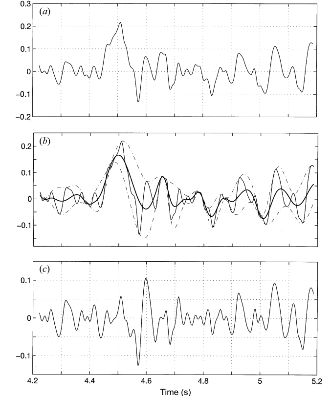
Figure 1: Illustration of Empirical Mode Decomposition (EMD). The goal of the EMD is to decompose a composite time series into the sum of identifiable oscillatory modes. (a) Original time series. (b) Average of the upper and lower envelopes formed by fitting extrema. (c) By subtracting the average from the time series, we extract the highest frequency mode. This mode is further refined by the same procedure until a single, stable oscillatory mode is obtained. The mode is removed from the data (not shown), and the entire procedure is repeated on the remainder to obtain additional lower frequency modes.

The HSA derives the instantaneous frequency ($I\!F$) and amplitude ($I\!A$) at each time by differentiating the phase and taking the absolute value of the analytical complex representation of each IMF, obtained with the IMF itself (real part) and the Hilbert transform of the IMF (imaginary part). The IF and IA are then, essentially, the frequency and amplitude of the best fit sinusoidal wave at each point in time [4]. Through this procedure the HHT allows extraction of instantaneous time-frequency and time-amplitude trajectories, in contrast to integral methods like Fourier or Wavelet analysis which are limited fundamentally by time-frequency spreading [5]. This instantaneous character of the HHT maps allows for high resolution time-frequency analysis, and in particular allows the detailed, high precision study of waveforms with strong frequency modulation. The HHT has been applied to the time series analysis of heart rate monitors [6], studies of electroencephalograms [7], investigations into the integrity of structures [8], and measurements of the seismic surface wave dispersion [9].

Time series analysis is now used in the search for gravitational wave (GW) sources. A number of high sensitivity detectors, including the US Laser Interferometer Gravitational Wave Observatory (LIGO)[10, 11], consisting of a 4 km detector in Louisiana and a 4 km and a 2 km detector in Washington, the European Virgo Observatory [12], consisting of a 3 km detector in Pisa, Italy, and the GEO600 observatory [13] consisting of a 600m detector near Sarstedt, Germany, are now in operation and analyzing data. A key concept in the data analysis is that the coincident appearance of signals in two or more detectors will be important in discriminating a real GW signal from an instrumental artifact. Signal comparison is also required in order to establish the relative timing of the appearance of an event in multiple widely-separated detectors so that the sky position of a possible source may be determined.

In this paper we demonstrate the use of instantaneous time-frequency maps provided by the HHT for relative signal timing, for use as a veto of accidental noise coincidences, and to characterize the time-frequency structure of transient instrumental noise artifacts (known as “glitches”) in recorded gravitational wave data. In all these studies frequency modulation plays an important role. We show these results using gravitational-wave data from the fourth science run of the Laser Interferometer Gravitational wave Observatory (LIGO S4) [14], which took place in early 2005. The S4 data run spanned two months and had detector sensitivities within a factor of two of the design goal.

The paper is organized as follows: in Sec. 2 we summarize the application of the HHT to this study. We show empirically in Sec. 3 that the measurement errors in the instantaneous amplitude and frequency provided by the HHT are a simple function of the local signal-to-noise ratio and are approximately Gaussian. This allows the use of a $\chi^{2}$ goodness-of-fit method to evaluate the match between time-frequency and time-amplitude maps, which can be applied to simulated signals as well as noise transients in S4 data. Sec. 4 shows the performance of relative timing between two common signals in noise obtained by minimizing the $\chi^{2}$ as a function of relative time delay. The use of the $\chi^{2}$ test to veto similar but unequal waveforms that could be caused by coincident noise transients is studied in Sec. 5, and grouping of instrumental artifacts into classes based on time-frequency and time-amplitude structure (glitch morphology) is discussed in Sec. 6.

2 Application of the Hilbert-Huang Transform in this work

We use an application of the HHT algorithm as described in [15] to analyze GW data with low integrated signal-to-noise ratio, SNR = $\sqrt{\sum_{i}h_{i}^{2}}/s$, where $s$ is the standard deviation of the discrete stationary noise in the time series after whitening and $h_{i}$ is the discrete (whitened) measured strain of the signal. This application uses Bayesian blocking [16] to identify regions of excess power in the instantaneous amplitude ($I\!A$), and uses the FFT-derived power spectrum of these regions to establish the maximum frequency of the event. It then low-pass filters the data at a frequency close to this maximum frequency to reduce distortion of the data from noise at frequencies greater than those contained in the signal. It performs a final processing technique (EEMD, [17]) to average over errors in the EMD process.

In this study we have made the following modifications to the HHT application to the GW data described above:

• The extrema of a time-sampled signal can occur between two distinct sampling points and thus may not be present in the discretized time series. The standard EMD uses the sampling point closest to the true extrema as the contact point for the upper envelope, leading to a false offset in magnitude and time. In this case, the mean of the data is underestimated, which leads to a decomposition error in the final IMF. This error manifests as a frequency modulation in the $I\!F$ and an amplitude modulation in the $I\!A$, seen as a sinusoidal oscillation around the true value with a period equal to the separation of the extrema in time. To correct for this we interpolate the data around the extrema with a cubic spline, and derive analytically the zero crossing of the first derivative of the spline in order to establish the true extrema of the data. The interpolated value in time and magnitude replaces the false extrema.

• For more stable results, and to capture the complete frequency content of an event within the dyadic frequency range of the first IMF, we have found that it is best to use a low-pass filter with frequency cut-off at twice the estimated maximum Fourier frequency of the signal.

3 Comparison of signals: instantaneous time-amplitude and time-frequency maps, associated errors, and their use in a $\chi^{2}$ goodness-of-fit measure

A quantitative comparison of time-frequency maps of signals from different detectors can form a basis for estimating relative signal timing, and the likelihood of the signals being consistent. We approach the problem of comparison of signals from different detectors through the use of a $\chi^{2}$ goodness-of-fit measure between the instantaneous time-amplitude and time-frequency maps of the signals generated by the application of the HHT to the time series data.

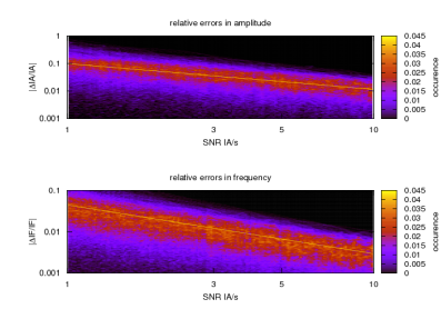
Figure 2: 2-D histogram of the absolute fractional uncertainties in the extraction of instantaneous frequencies and amplitudes of the HHT as a function of local signal-to-noise (SNR = $I\!A/s$) for a population of sine-Gaussian, BBH merger, and white noise burst signals. Occurence represents the percent occupancy of the population at fixed SNR. The 1$\sigma$ spread in the fractional measurements correspond to the most likely absolute fractional error in the log-scale binning on $|\Delta I\!F/I\!F|$. We find that the 1$\sigma$ uncertainties in $I\!A$ and $IF$ are well described by a power-law in normalized amplitude $I\!A/s$.

In this approach the degree of match of two signals from detectors 1 and 2 is determined by computing a reduced $\chi^{2}$ statistic using $I\!A$ and $I\!F$ ($N$ denoting the total number of sampling points in time)

$$\chi_{1,2}^{2}=\frac{1}{2N}\left[\sum_{n=1}^{N}\frac{(I\!A_{1}[n]-I\!A_{2}[n])^{2}}{\sigma_{I\!A_{1}}^{2}[n]+\sigma_{I\!A_{2}}^{2}[n]}+\sum_{n=1}^{N}\frac{(I\!F_{1}[n]-I\!F_{2}[n])^{2}}{\sigma_{I\!F_{1}}^{2}[n]+\sigma_{I\!F_{2}}^{2}[n]}\right],$$ (1)

where $\sigma[n]$ is the uncertainty in the $I\!A$ or $I\!F$, both of which are time-dependent functions of $I\!A$. For this test, $I\!A$ is also normalized by its maximum absolute value so that the test is sensitive only to the shape of the $I\!A$ evolution and not the absolute magnitude. This is important, for example, in the case of a gravitational-wave which may be subject to different antenna scaling factors from misaligned detectors, as well as amplitude errors in detector calibration. $2N$ does not denote the effective number of degrees of freedom in this reduced $\chi^{2}$ because of correlations between the data points, which are generally sampled at a much higher rate than twice the bandwidth of data contained in the IMFs. In practice an empirical threshold on the reduced $\chi^{2}$ is determined through Monte Carlo studies to limit the false-dismissal rate for identical signals to 1$\%$ or less.

The fractional uncertainty for the $I\!A$ and $I\!F$ produced by the HHT is related at each point in time to the measured ratio $I\!A/s$, where $s$ here refers to the standard devation of the white noise within the IMF band. In general a larger $I\!A/s$ yields a smaller fractional uncertainty. We determine these uncertainties by injecting a variety of ad-hoc signals used in the LIGO S4 burst search [14] as well as waveforms from numerical relativity into white Gaussian noise, with the SNR of these signals ranging from 1 to 30. These signals include sine-Gaussians with frequencies ranging from 60 Hz to 3 kHz and quality factors, Q (number of cycles), from 3 to 9, two equal mass binary black hole (BBH) merger signals [18, 19] with total system masses of 20 and 60 $M_{\odot}$ and ring-down frequencies (oscillation frequency of the resulting black hole after merger) of 400 and 250 Hz respectively, and white noise bursts consisting of band passed noise with a flat spectral density between 100 and 200 Hz and a Gaussian time-envelope with a width of 1, 10 and 100 ms. We then use the HHT to extract the $I\!A$ and $I\!F$ for each signal, and obtain the fractional uncertainty by comparing the $I\!A$ and $I\!F$ with the values seen in zero noise (see Fig. 2). The $1\sigma$ $I\!A$ uncertainty and the $1\sigma$ $I\!F$ uncertainty versus measured $I\!A/s$ is found by fitting a straight line to the most likely absolute fractional uncertainty in the log-log plane, so that the fractional uncertainty takes the form of a power law in $I\!A/s$,

$$\log_{10}(\sigma_{I\!A})\approx-1.12\cdot\log_{10}(I\!A/s)-0.52$$ (2)

$$\log_{10}(\sigma_{I\!F})\approx-0.60\cdot\log_{10}(I\!A/s)-0.28$$ (3)

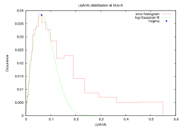
Figure 3: Histogram of absolute fractional uncertainties in IA for a population of simulated signals at IA/s=5, and a one-sided Gaussian fit to the distribution with corresponding 1$\sigma$ indicated. Due to the log-scale binning in $|\Delta IA/IA|$, the 1$\sigma$ spread in the one-sided distribution corresponds to maximum occurance. The histogram is normalized to 1.

We assign these uncertainties to the extraction of $I\!A$ and $I\!F$ from LIGO data by referring the ratio $I\!A/s$ at each data point to these linear fits. We find the uncertainties to be roughly Gaussian distributed at any value of $I\!A/s$, but to also have non-Gaussian features towards higher $I\!A/s$ (see Fig. 3).

4 Timing with the $\chi^{2}$ statistic

The relative timing of signals from a network of gravitational wave detectors can be used to determine the sky location of the astrophysical source of a gravitational wave signal (e.g. [20])]. The $\chi^{2}$ goodness-of-fit measure can be used for timing the arrival of common signals by time shifting one detector time series with respect to the other by small intervals up to a total of $\pm 10$ ms (the maximum travel time of a GW between the LIGO sites), calculating the $\chi^{2}$ for each time-shift, and noting the relative time-shift corresponding to the minimal $\chi^{2}$ value. This minimum then denotes the best overlap of the time-frequency and time-amplitude maps of the two detector data streams.

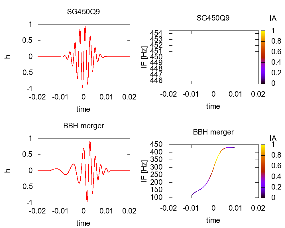
Figure 4: Signal waveforms and HHT-derived time-frequency maps for the signals used to test relative timing: sine-Gaussian f=450, Q=9 and a 20 $M_{\odot}$ BBH merger. The 66.7, 95.7, and 99.7 percentiles of the distribution of absolute time-shift error versus SNR are shown in the top panel.

To demonstrate this technique we use two test waveforms: the binary black hole merger with total mass 20 $M_{\odot}$ and a sine-Gaussian of frequency 450 Hz and Q of 9. The waveforms and instantaneous time-frequency maps of these signals are shown in Fig. 4. Fig. 5 shows the reduced $\chi^{2}$ versus time-shift for the two waveforms when injected into different realizations of Gaussian white noise at SNR = 20. The injections were also performed multiple times with varying SNR. At each SNR, we note the spread of the relative timing measurements obtained by minimizing the $\chi^{2}$ versus time-shift. The 66.7, 95.7, and 99.7 percentiles (1, 2, and 3$\sigma$ respectively) of the distribution of absolute time-shift error versus SNR are shown in Fig. 5. As expected, we observe an improvement in timing with rising SNR. Overall the binary black hole merger shows superior relative timing to the sine-Gaussian waveform as the sine-Gaussian’s flat frequency profile at 450 Hz reduces the contrast of the $\chi^{2}$ with respect to small time-shifts. For the back hole merger waveform at SNR=10, the 1$\sigma$ relative timing error between two detectors is $\sim$0.5 ms, which is comparable with matched filter methods [21].

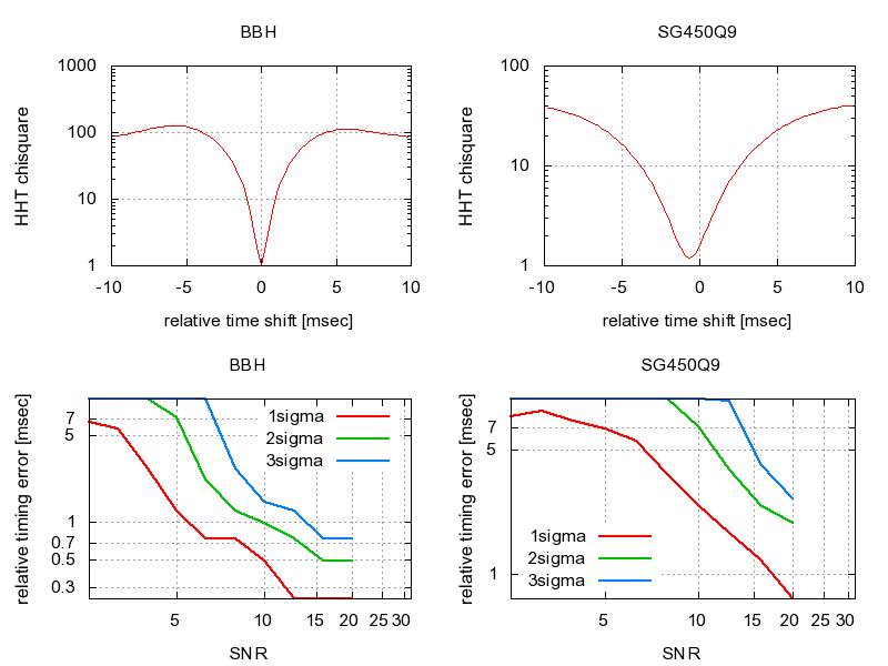
Figure 5: Top panels: $\chi^{2}$ comparison of time-frequency and time-amplitude maps versus time-shift for a single SNR=20 $M_{\odot}$ BBH merger (left) and sine-Gaussian 450Hz Q9 (right) waveform injected in both detectors. The true difference in arrival time is estimated by locating the minimum $\chi^{2}$ value. Lower panels: the aggregate relative timing errors obtained for these waveforms as a function of SNR. The 66.7, 95.7, and 99.8 percentiles for the distribution of absolute timing errors are shown for an ensemble of injections.

5 Vetoing unequal waveforms with instantaneous time-frequency maps

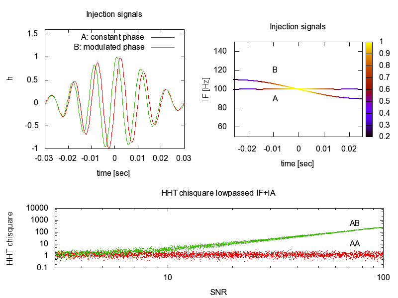
Figure 6: The HHT $\chi^{2}$ goodness of fit is used to differentiate very similar waveforms, for use in veto strategies of instrumental noise coincidences between two gravitational wave detectors. We display the $\chi^{2}$ comparison of two waveforms, with one of constant frequency (A) and the other phase modulated at 1/10th of the base frequency (B). The two waveforms have a linear correlation coefficient of 0.96. The top left panel shows the waveforms. The top right panel shows the $I\!F$ of each waveform versus time, with $I\!A$ color coded. The lower panel is a scatter plot of reduced $\chi^{2}$ values between waveforms A and B (green) and identical waveform A and A (red) as a function of SNR. By applying a reduced $\chi^{2}$ threshold of 2.7, waveforms A and B can be distinguished 63% of the time at SNR=7, and 93% of the time at SNR=10 while maintaining a false-dismissal probability of 1% or lower for identical waveforms.

The HHT $\chi^{2}$ goodness of fit applied to $I\!A$ and $I\!F$ can also be used to veto similar but unequal waveforms. Thus it may be used for veto strategies that seek to reject instrumental noise coincidences of signals which are closely related but not identical. To illustrate the HHT $\chi^{2}$ veto, we consider the following very similar waveforms:

• waveform A: $\sin\left(2\pi 100t\right)\exp\left[\frac{(2\pi 100t)^{2}}{2\cdot 9^{2}}\right]$

• waveform B: $\sin\left(2\pi 100t+\cos(2\pi 10t)\right)\exp\left[\frac{(2\pi 100t)^{2}}{2\cdot 9^{2}}\right]$

The second waveform is chosen to have a 10 Hz cosine phase modulation with respect to the 100 Hz base frequency of the first, as low frequency modulations about a 100 Hz base frequency are often seen in instrumental glitches (see Section 6). Both waveforms have a Gaussian amplitude and a Q$\sim$9. The linear correlation coefficient $\left[\sum{(h_{A}-\bar{h}_{A})(h_{B}-\bar{h}_{B})}\right]/\sqrt{\sum{(h_{A}-\bar{h}_{A})^{2}}\sum{(h_{B}-\bar{h}_{B})^{2}}}$ of the waveforms is 0.96 (0 is uncorrelated while 1 is fully correlated), indicating a very high degree of similarity. These waveforms are injected into white Gaussian noise at varying SNR (see Fig. 6). By setting a threshold in the reduced $\chi^{2}$ of 2.7, the waveforms A and B can be shown to be dissimilar and thus vetoed 63% of the time at SNR = 7, vetoed 93% of the time at SNR = 10, and vetoed essentially 100% of the time at SNR = 15. The false rejection probability, determined by applying this veto procedure to identical waveforms (i.e. A and A) is 1% or less over the full range of SNR.

6 Glitch morphology of S4 data

In this section we use the comparison of time-frequency maps of instrumental noise artifacts (known as “glitches”) from the GW channel of the Livingston 4 km detector (L1) during S4 in order to group them into classes whose members contain similar time-frequency structure; the goal is that these groupings may correspond to specific physical mechanisms which cause the disturbance. We refer to this grouping as establishing a “morphology” of the glitches. Instrumental noise artifacts are first identified in the S4 science data (after data quality [14] cuts have been applied) by using the KleineWelle (KW) algorithm [22] which searches for excess signal power in the wavelet domain. Triggers are required to be isolated with no other trigger within 1 second to simplify signal comparison, and are also required to be of sufficient strength (SNR$\gtrsim$8.7) for precise time-frequency reconstruction. We apply the $\chi^{2}$ test on these events in order to find glitches with similar time-frequency and time-amplitude trajectories, which we then group into the same morphology class. We consider two events to be in the same class if their reduced $\chi^{2}$ is less than 2.

To illustrate this approach, we present four of the 14 most populated glitch classes, summarized in Table 1. Each class contains more than 10 individual members, and are chosen for their degree of match across class members or common association with auxiliary interferometric channels. For example we show in Fig. 7 three members of class 1. The similar time-frequency structure is present throughout the 31 members of this class. As seen in these three examples, the glitches can show complicated structure consisting of more than one oscillatory mode. These modes are separated by the EMD procedure, and they are shown by separate traces on the time-frequency maps. The weaker mode in this particular example is centered at 50 Hz with fairly low modulation, while the stronger mode shows stronger frequency modulation peaking at around 100 Hz. The detailed frequency modulation of the modes is represented by the time-frequency traces, with errors (obtained through the application of Eq. 2) shown as grey bands.

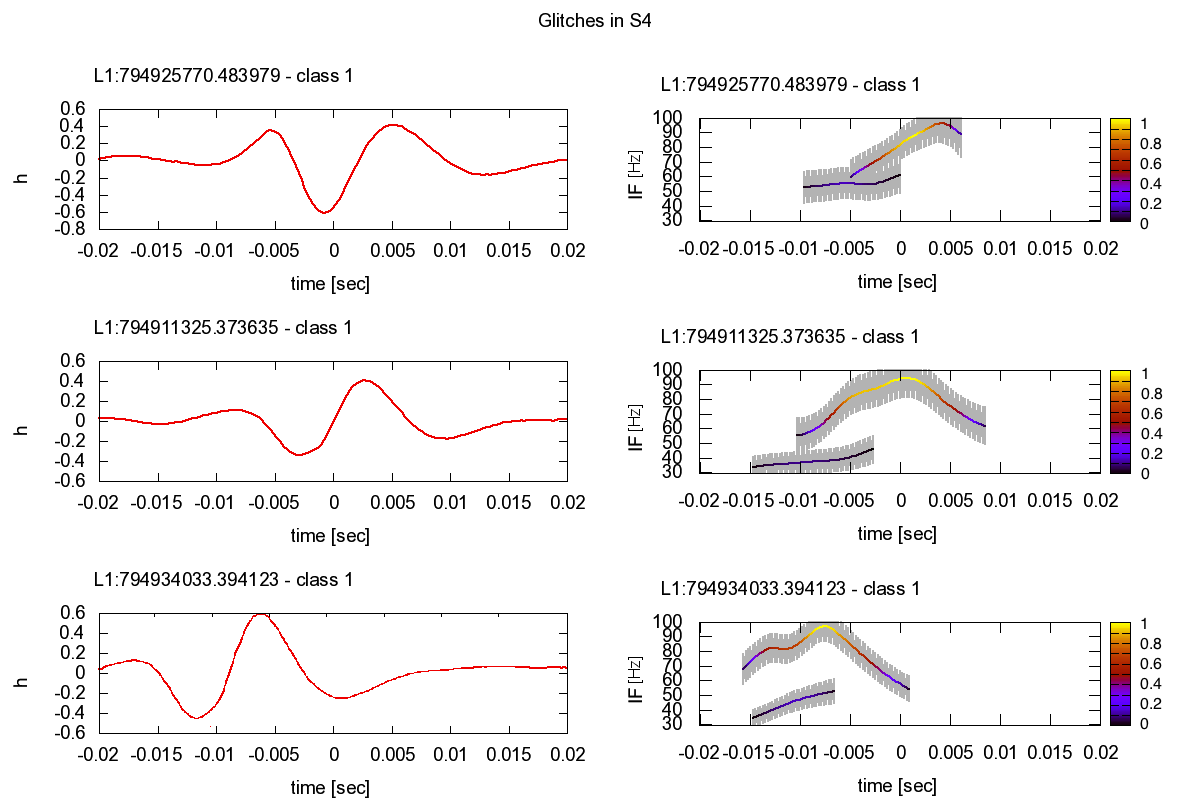
Figure 7: Three members of glitch morphology class 1 are displayed with their time-frequency maps. $I\!A(t)$ is indicated by the color scale, and uncertainties in measured $I\!F$ are indicated as grey shading. The time-frequency structure of the two modes of this glitch class is present throughout the 31 members.

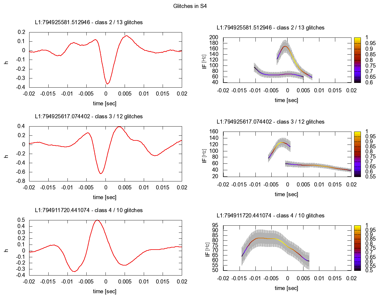
Figure 8: An individual example from each of three different glitch classes which show evidence of a link to auxiliary channels. Left panels show the whitened time series, right panels show the time-frequency maps with $I\!F(t)$ with $I\!A(t)$ indicated by the color scale, and uncertainties in measured $I\!F$ indicated as grey shading.

We also show in Fig. 8 a comparison of the time-frequency structures of the glitches from three additional classes 2, 3, and 4. The time-frequency map of class 2 in Fig. 8 consists of two physical modes, one around 60 Hz with a shallow frequency modulation, and one peaking at 180 Hz with a stronger modulation. These modes can also be seen in the time series of the glitch, where a slower oscillation is superimposed on top of a faster, larger oscillation around $t=0$. Class 3 consists of two physical modes at 120 and 60 Hz, while class 4 appears to be a single physical mode at 80 Hz.

After establishing glitch morphology classes, we look for correlations of the different classes with auxiliary channels. This is done by looking for time coincidences of KW auxiliary channel triggers within a 50 ms window about the peak time of the GW channel trigger. In morphology classes 2, 3 and 4, more than 50% of the members can be associated with a simultaneous transient disturbance in a channel related to the control of the interferometer (PRC), a channel related to the alignment of an interferometer test mass (WFS), or a channel related to the intensity of light picked off from the beam splitter (POB). These correlations are detailed in Tab. 1.

The overall goal of grouping of the glitches into these classes is to obtain insight into the physical processes producing them. So far achieving this goal remains elusive in S4 data. The modes and frequency modulations shown in Fig. 7 do not easily suggest any physical mechanism. Nevertheless, their common time-frequency structure indicates some underlying cause. We believe that the cataloging of groups of glitches based on time-frequency structure, and the ongoing correlation of these classes with auxiliary channels, is a useful first step to understanding and ultimately removing them.

Morphology class	member count	remarks
1	31	60 % PRC; 52 % POB
2	13	62 % PRC; 54 % POB
3	12	50% WFS, 50% POB
4	10	50 % POB

Table 1: A glitch morphology study on S4 data in the Livingston 4km detector. Four of the 14 most populated glitch morphology classes are tabulated which demonstrate consistent time-frequency structure or association with auxiliary interferometric channels. Individual members from each class can be found in Figures 7 and 8.

7 Conclusions

In this study we showed how instantaneous time-frequency and time-amplitude maps, as provided by the Hilbert-Huang Transform, can be used to determine the relative timing of signals in a network of gravitational-wave detectors, to enable a veto that can discriminate between similar but unequal waveforms, and to group instrumental artifacts based on their time-frequency trajectories. The $\chi^{2}$ goodness-of-fit test proposed provides a measure of comparison of the time-frequency and time-amplitude maps. The high time resolution of the instantaneous maps allows strong frequency modulations to be addressed in a straightforward way, a critical factor in gaining insight into the physical nature of the signals and instrumental artifacts.

Future research will concentrate on the errors in the HHT $I\!F$ and $I\!A$ extraction, with the goal of understanding their origin and minimizing their magnitude. These errors impact the effectiveness of the timing and veto estimates directly, and also affect the level of discrimination of the glitch morphology groupings.

References

References

- [1] N.E. Huang and S.S. Shen. Hilbert-Huang Transform and Its Applications. World Scientific, 2005.
- [2] N.E. Huang, Z. Shen, S.R. Long, M.C. Wu, H.H. Shih, Q. Zheng, N.C. Yen, C.C. Tung, and H.H. Liu. The empirical mode decomposition and the Hilbert spectrum for nonlinear and non-stationary time series analysis. Proceedings-Royal Society of London A, 454:903–995, 1998.
- [3] Z. Wu and N.E. Huang. A study of the characteristics of white noise using the empirical mode decomposition method. Proceedings of the Royal Society A: Mathematical, Physical and Engineering Sciences, 460(2046):1597–1611, 2004.
- [4] Leon Cohen. Time-frequency analysis: theory and applications, chapter 2. Prentice-Hall, Inc., Upper Saddle River, NJ, USA, 1995.
- [5] N. E. Huang, Z. Wu, S.R. Long, K.C. Arnold, and X. Chen. On instantaneous frequency. AADA, 2, 2009. in press.
- [6] Xiao-Li Yang; Jing-Tian Tang;. Hilbert-huang transform and wavelet transform for ecg detection. Wireless Communications, Networking and Mobile Computing, 2008. WiCOM ’08, 1:1–4, 12-14 Oct. 2008.
- [7] Zhong xing Zhou, Bai kun Wan, Dong Ming, and Hong zhi Qi. A novel technique for phase synchrony measurement from the complex motor imaginary potential of combined body and limb action. Journal of Neural Engineering, 7(4):046008, 2010.
- [8] WH Chen JS Jiang L Yu HG Chen, YJ Yan and ZY Wu. Early damage detection in composite wingbox structures using hilbert-huang transform and genetic algorithm. struct health monit, 6:281, 2007.
- [9] Ta-Liang Teng Chau-Huei Chen, Cheng-Ping Li. Surface-wave dispersion measurements using hilbert-huang transform. TAO, 13:2171–184, 2002.
- [10] A. Abramovici, W.E. Althouse, R.W.P. Drever, Y. Gursel, S. Kawamura, F.J. Raab, D. Shoemaker, L. Sievers, R.E. Spero, K.S. Thorne, et al. LIGO: The Laser Interferometer Gravitational-Wave Observatory. Science, 256(5055):325–333, 1992.
- [11] BC Barish and R. Weiss. LIGO and the detection of gravitational waves. Phys. Today, 52(10), 1999.
- [12] C. Bradaschia, R. del Fabbro, A. di Virgilio, A. Giazotto, H. Kautzky, V. Montelatici, D. Passuello, A. Brillet, O. Cregut, P. Hello, et al. The VIRGO Project: A wide band antenna for gravitational wave detection. Nuclear Instruments and Methods in Physics Research Section A, 289(3), 1990.
- [13] B Willke et al.. The GEO 600 gravitational wave detector Classical and Quantum Gravity, 19:1377–1387, 2002.
- [14] LIGO Scientific Collaboration B Abbott et al. First joint search for gravitational-wave bursts in ligo and geo 600 data. Classical and Quantum Gravity, 25(24):245008, 2008.
- [15] A. Stroeer, J. K. Cannizzo, J. B. Camp, and N. Gagarin. Methods for detection and characterization of signals in noisy data with the Hilbert-Huang transform. Physical Review D, 79(12):124022–+, June 2009.
- [16] JWC McNabb, M. Ashley, LS Finn, E. Rotthoff, A. Stuver, T. Summerscales, P. Sutton, M. Tibbits, K. Thorne, and K. Zaleski. Overview of the BlockNormal event trigger generator. Classical and Quantum Gravity, 21:1705–1710, 2004.
- [17] Z. Wu, N.E. Huang, and Center for Ocean-Land-Atmosphere Studies. Ensemble Empirical Mode Decomposition: A Noise Assisted Data Analysis Method. Center for Ocean-Land-Atmosphere Studies, 2005.
- [18] J.G. Baker, J. Centrella, D.I. Choi, M. Koppitz, and J. van Meter. Binary black hole merger dynamics and waveforms. Physical Review D, 73(10):104002, 2006.
- [19] J.G. Baker, J. Centrella, D.I. Choi, M. Koppitz, and J. van Meter. Gravitational-Wave Extraction from an Inspiraling Configuration of Merging Black Holes. Physical Review Letters, 96(11):111102, 2006.
- [20] J. Markowitz, M. Zanolin, L. Cadonati, and E. Katsavounidis. Gravitational wave burst source direction estimation using time and amplitude information. Phys. Rev. D, 78(12):122003, Dec 2008.
- [21] S. Vitale and M. Zanolin. Parameter estimation from Gravitational waves generated by non-spinning binary black holes with laser interferometers: beyond the Fisher information. ArXiv e-prints, April 2010.
- [22] S. Chatterji, L. Blackburn, G. Martin, and E. Katsavounidis. Multiresolution techniques for the detection of gravitational-wave bursts. Class. Quant. Grav., 21:S1809–S1818, 2004.