Uniqueness and universality of the Brownian map

Abstract

We consider a random planar map $M_{n}$ which is uniformly distributed over the class of all rooted $q$-angulations with $n$ faces. We let $\mathbf{m}_{n}$ be the vertex set of $M_{n}$, which is equipped with the graph distance $d_{\mathrm{gr}}$. Both when $q\geq 4$ is an even integer and when $q=3$, there exists a positive constant $c_{q}$ such that the rescaled metric spaces $(\mathbf{m}_{n},c_{q}n^{-1/4}d_{\mathrm{gr}})$ converge in distribution in the Gromov–Hausdorff sense, toward a universal limit called the Brownian map. The particular case of triangulations solves a question of Schramm.

[alignleft,level=2]

1 Introduction

In the present work, we derive the convergence in distribution in the Gromov–Hausdorff sense of several important classes of rescaled random planar maps, toward a universal limit called the Brownian map. This solves an open problem that has been stated first by Oded Schramm Sch in the particular case of triangulations.

Recall that a planar map is a proper embedding of a finite connected graph in the two-dimensional sphere, viewed up to orientation-preserving homeomorphisms of the sphere. Loops and multiple edges are allowed in the graph. The faces of the map are the connected components of the complement of edges, and the degree of a face counts the number of edges that are incident to it, with the convention that if both sides of an edge are incident to the same face, this edge is counted twice in the degree of the face. Special cases of planar maps are triangulations, where each face has degree $3$, quadrangulations, where each face has degree $4,$ and, more generally, $q$-angulations, where each face has degree $q$. For technical reasons, one often considers rooted planar maps, meaning that there is a distinguished oriented edge whose origin is called the root vertex. Since the pioneering work of Tutte Tu , planar maps have been studied thoroughly in combinatorics, and they also arise in other areas of mathematics: See, in particular, the book of Lando and Zvonkin LZ for algebraic and geometric motivations. Large random planar graphs are of interest in theoretical physics, where they serve as models of random geometry ADJ , in particular, in the theory of two-dimensional quantum gravity.

Let us introduce some notation in order to give a precise formulation of our main result. Let $q\geq 3$ be an integer. We assume that either $q=3$ or $q$ is even. The set of all rooted planar $q$-angulations with $n$ faces is denoted by ${\mathcal{A}}^{q}_{n}$. For every integer $n\geq 1$ (if $q=3$ we must restrict our attention to even values of $n$, since ${\mathcal{A}}^{3}_{n}$ is empty if $n$ is odd), we consider a random planar map $\mathbf{M}_{n}$ that is uniformly distributed over ${\mathcal{A}}^{q}_{n}$. We denote the vertex set of $\mathbf{M}_{n}$ by $\mathbf{m}_{n}$. We equip $\mathbf{m}_{n}$ with the graph distance $d_{\mathrm{gr}}$, and we view $(\mathbf{m}_{n},d_{\mathrm{gr}})$ as a random variable taking values in the space $\mathbb{K}$ of isometry classes of compact metric spaces. We equip $\mathbb{K}$ with the Gromov–Hausdorff distance $d_{\mathrm{GH}}$ (see, e.g., BBI ) and note that $(\mathbb{K},d_{\mathrm{GH}})$ is a Polish space.

Theorem 1.1

Set

$$c_{q}=\biggl{(}\frac{9}{q(q-2)}\biggr{)}^{1/4}$$

if $q$ is even, and

$$c_{3}=6^{1/4}.$$

There exists a random compact metric space $(\mathbf{m}_{\infty},D^{*})$ called the Brownian map, which does not depend on $q$, such that

$$\bigl{(}\mathbf{m}_{n},c_{q}n^{-1/4}d_{\mathrm{gr}}\bigr{)}\mathrel{\mathop{\longrightarrow}\limits_{n\to\infty}^{\mathrm{(d)}}}\bigl{(}\mathbf{m}_{\infty},D^{*}\bigr{)},$$

where the convergence holds in distribution in the space $\mathbb{K}$.

Let us give a precise definition of the Brownian map. We first need to introduce the random real tree called the CRT, which can be viewed as the tree coded by a normalized Brownian excursion, in the following sense. Let $(\mathbf{e}_{s})_{0\leq s\leq 1}$ be a normalized Brownian excursion, that is, a positive excursion of linear Brownian motion conditioned to have duration $1$, and set, for every $s,t\in[0,1]$,

$$d_{\mathbf{e}}(s,t)=\mathbf{e}_{s}+\mathbf{e}_{t}-2\min_{s\wedge t\leq r\leq s\vee t}\mathbf{e}_{r}.$$

Then $d_{\mathbf{e}}$ is a (random) pseudometric on $[0,1]$, and we consider the associated equivalence relation $\sim_{\mathbf{e}}$: for $s,t\in[0,1]$,

$$s\sim_{\mathbf{e}}t\quad\mbox{if and only if}\quad d_{\mathbf{e}}(s,t)=0.$$

Since $0\sim_{\mathbf{e}}1$, we may as well view $\sim_{\mathbf{e}}$ as an equivalence relation on the unit circle ${\mathbb{S}}^{1}$. The CRT is the quotient space ${\mathcal{T}}_{\mathbf{e}}:={\mathbb{S}}^{1}/\sim_{\mathbf{e}}$, which is equipped with the distance induced by $d_{\mathbf{e}}$. We write $p_{\mathbf{e}}$ for the canonical projection from ${\mathbb{S}}^{1}$ onto ${\mathcal{T}}_{\mathbf{e}}$, and $\rho=p_{\mathbf{e}}(1)$. If $u,v\in{\mathbb{S}}^{1}$, we let $[u,v]$ be the subarc of ${\mathbb{S}}^{1}$ going from $u$ to $v$ in clockwise order, and if $a,b\in{\mathcal{T}}_{\mathbf{e}}$, we define $[a,b]$ as the image under the canonical projection $p_{\mathbf{e}}$ of the smallest subarc $[u,v]$ of ${\mathbb{S}}^{1}$ such that $p_{\mathbf{e}}(u)=a$ and $p_{\mathbf{e}}(v)=b$. Roughly speaking, $[a,b]$ corresponds to the set of vertices that one visits when going from $a$ to $b$ around the tree in clockwise order.

We then introduce Brownian labels on the CRT. We consider a real-valued process $Z=(Z_{a})_{a\in{\mathcal{T}}_{\mathbf{e}}}$ indexed by the CRT, such that, conditionally on ${\mathcal{T}}_{\mathbf{e}}$, $Z$ is a centered Gaussian process with $Z_{\rho}=0$ and $E[(Z_{a}-Z_{b})^{2}]=d_{\mathbf{e}}(a,b)$ (this presentation is slightly informal as we are considering a random process indexed by a random set, see Section 2.4 for a more rigorous approach). We define, for every $a,b\in{\mathcal{T}}_{\mathbf{e}}$,

$$D^{\circ}(a,b)=Z_{a}+Z_{b}-2\max\Bigl{(}\min_{c\in[a,b]}Z_{c},\min_{c\in[b,a]}Z_{c}\Bigr{)},$$

and we put $a\simeq b$ if and only if $D^{\circ}(a,b)=0$. Although this is not obvious, it turns out that $\simeq$ is an equivalence relation on ${\mathcal{T}}_{\mathbf{e}}$, and we let

$$\mathbf{m}_{\infty}:={\mathcal{T}}_{\mathbf{e}}/\simeq$$

be the associated quotient space. We write $\Pi$ for the canonical projection from ${\mathcal{T}}_{\mathbf{e}}$ onto $\mathbf{m}_{\infty}$. We then define the distance on $\mathbf{m}_{\infty}$ by setting, for every $x,y\in\mathbf{m}_{\infty}$,

$$D^{*}(x,y)=\inf\Biggl{\{}\sum_{i=1}^{k}D^{\circ}(a_{i-1},a_{i})\Biggr{\}},$$ (1)

where the infimum is over all choices of the integer $k\geq 1$ and of the elements $a_{0},a_{1},\ldots,a_{k}$ of ${\mathcal{T}}_{\mathbf{e}}$ such that $\Pi(a_{0})=x$ and $\Pi(a_{k})=y$. It follows from IM , Theorem 3.4, that $D^{*}$ is indeed a distance, and the resulting random metric space $(\mathbf{m}_{\infty},D^{*})$ is the Brownian map.

The present work can be viewed as a continuation and in a sense a conclusion to our preceding papers IM and AM . In IM , we proved the existence of sequential Gromov–Hausdorff limits for rescaled uniformly distributed rooted $2p$-angulations with $n$ faces, and we called a Brownian map any random compact metric space that can arise in such limits (the name Brownian map first appeared in the work of Marckert and Mokkadem MM which was dealing with a weak form of the convergence of rescaled quadrangulations). The main result of IM used a compactness argument that required the extraction of suitable subsequences in order to get the desired convergence. The reason why this extraction was needed is the fact that the limit could not be characterized completely. It was proved in IM that any Brownian map can be written in the form $(\mathbf{m}_{\infty},D)$, where the set $\mathbf{m}_{\infty}$ is as described above, and $D$ is a distance on $\mathbf{m}_{\infty}$, for which only upper and lower bounds were available in IM , AM . In particular, the paper IM provided no characterization of the distance $D$ and it was conceivable that different sequential limits, or different values of $q$, could lead to different metric spaces. In the present work, we solve this uniqueness problem by establishing the explicit formula (1), which had been conjectured in IM and in a slightly different form in MM . As a consequence, we obtain the uniqueness of the Brownian map, and we get that this random metric space is the scaling limit of uniformly distributed $q$-angulations with $n$ faces, for the values of $q$ discussed above. Our proofs strongly depend on the study of geodesics in the Brownian map that was developed in AM .

At this point, one should mention that the very recent paper of Miermont Mi-quad has given another proof of Theorem 1.1 in the special case of quadrangulations ($q=4$). Our approach was developed independently of Mi-quad and uses very different ingredients, leading to more general results. On the other hand, the proof in Mi-quad gives additional information about the properties of geodesics in $\mathbf{m}_{\infty}$, which is of independent interest.

Let us briefly sketch the main ingredients of our proof in the bipartite case where $q$ is even. From the main theorem of IM , we can find sequences $(n_{k})_{k\geq 1}$ of integers converging to $\infty$ such that the random metric spaces $(\mathbf{m}_{n_{k}},c_{q}n_{k}^{-1/4}d_{\mathrm{gr}})$ converge in distribution to $(\mathbf{m}_{\infty},D)$, where $D$ is a distance on $\mathbf{m}_{\infty}$ such that $D\leq D^{*}$. Additionally, the space $(\mathbf{m}_{\infty},D)$ comes with a distinguished point $x_{*}$, which is such that, for every $y\in\mathbf{m}_{\infty}$, and every $a\in{\mathcal{T}}_{\mathbf{e}}$ such that $\Pi(a)=y$,

$$D(y,x_{*})=D^{*}(y,x_{*})=Z_{a}-\min Z.$$

The heart of the proof is now to verify that $D=D^{*}$ (Theorem 7.2 below). To this end, it is enough to prove that $D(y,y^{\prime})=D^{*}(y,y^{\prime})$ a.s. when $y$ and $y^{\prime}$ are distributed uniformly and independently on $\mathbf{m}_{\infty}$ (the word uniformly refers to the volume measure on $\mathbf{m}_{\infty}$, which is the image of the normalized Lebesgue measure on $\mathbb{S}^{1}$ under the projection $\Pi\circ p_{\mathbf{e}}$). By the results in AM , it is known that there is an almost surely unique geodesic path $(\Gamma(t),0\leq t\leq D(y,y^{\prime}))$ from $y$ to $y^{\prime}$ in the metric space $(\mathbf{m}_{\infty},D)$.

Proving that $D(y,y^{\prime})=D^{*}(y,y^{\prime})$ is then essentially equivalent to verifying that the geodesic $\Gamma$ is well approximated (in the sense that the lengths of the two paths are not much different) by another continuous path going from $y$ to $y^{\prime}$, which is constructed by concatenating pieces of geodesics toward the distinguished point $x_{*}$. To this end, we prove that, for every choice of $r\geq\varepsilon>0$, and conditionally on the event $\{D(y,y^{\prime})\geq r+\varepsilon\}$, the probability that we have either

$$D\bigl{(}x_{*},\Gamma(r)\bigr{)} = D\bigl{(}x_{*},\Gamma(r+\varepsilon)\bigr{)}+\varepsilon\quad\mbox{or}$$

$$D\bigl{(}x_{*},\Gamma(r)\bigr{)} = D\bigl{(}x_{*},\Gamma(r-\varepsilon)\bigr{)}+\varepsilon$$

is bounded below by $1-\varepsilon^{\beta}$ when $\varepsilon$ is small, where $\beta>0$ is a constant. If (1) holds, this means that there is a geodesic from $x_{*}$ to $\Gamma(r)$ that visits either $\Gamma(r-\varepsilon)$ or $\Gamma(r+\varepsilon)$ and then coalesces with $\Gamma$. This is of course reminiscent of the results of AM saying that any two geodesic paths (starting from arbitrary points of $\mathbf{m}_{\infty}$) ending at a “typical” point $x$ of $\mathbf{m}_{\infty}$ must coalesce before hitting $x$. The difficulty here comes from the fact that interior points of geodesics are not typical points of $\mathbf{m}_{\infty}$ and so one cannot immediately rely on the results of AM to establish the preceding estimate (though these results play a crucial role in the proof).

As in many other papers investigating scaling limits for large random planar maps, our proofs make use of bijections between planar maps and various classes of labeled trees. In the bipartite case, we rely on a bijection discovered by Bouttier, Di Francesco and Guitter BDG between rooted and pointed $2p$-angulations with $n$ faces and labeled $p$-trees with $n$ black vertices (see Section 2.1, in the case of triangulations we use another bijection from BDG , which is presented in Section 8.1). A variant of this bijection allows us to introduce the notion of a discrete map with geodesic boundaries (DMGB in short), which, roughly speaking, corresponds to cutting the map along a particular discrete geodesic from the root vertex to the distinguished vertex. This cutting operation produces two distinguished geodesics, which are called the boundary geodesics. The notion of a DMGB turns out to play an important role in our proofs and is also of independent interest. The general philosophy of our approach is that a large planar map can be obtained by gluing together many DMGBs along their boundary geodesics.

To complete this introduction, let us mention that the idea of studying the continuous limit of large random quadrangulations first appeared in the pioneering paper of Chassaing and Schaeffer CS , which obtained detailed information about the asymptotics of distances from the root vertex. The results of Chassaing and Schaeffer were extended to more general classes of random maps in several papers of Miermont and his coauthors (see, in particular, MaMi , MieInvar ), using the bijections with trees found in BDG . All these results are concerned with the profile of distances from a particular vertex of the graph and do not provide enough information to understand Gromov–Hausdorff limits. The understanding of these limits would be possible if one could compute the asymptotic $k$-point function, that is, the asymptotic distribution of the matrix of mutual distances between $k$ randomly chosen vertices. In the particular case of quadrangulations, the asymptotic $2$-point function can be derived from the results of CS , and the asymptotic $3$-point function has been computed by Bouttier and Guitter BG0 . However, the extension of these calculations to higher values of $k$ seems a difficult problem.

As a final remark, Duplantier and Sheffield DS recently developed a mathematical approach to two-dimensional quantum gravity based on the Gaussian free field. It is expected that this approach should be related to the asymptotics of large planar maps. The very recent paper She contains several conjectures in this direction. Another very appealing related question is concerned with canonical embeddings of the Brownian map: It is known LGP that the space $(\mathbf{m}_{\infty},D^{*})$ is a.s. homeomorphic to the $2$-sphere ${\mathbb{S}}^{2}$, and one may look for a canonical construction of a random distance $d$ on ${\mathbb{S}}^{2}$ such that $(\mathbf{m}_{\infty},D^{*})$ is a.s. isometric to $({\mathbb{S}}^{2},d)$. The random distance $d$ is expected to have nice conformal invariance properties. Hopefully these questions will lead to a promising new line of research in the near future.

The paper is organized as follows. Section 2 recalls basic facts about the coding of $2p$-angulations by labeled trees, and known results from IM and AM about the convergence of rescaled $2p$-angulations. Section 3 discusses discrete maps with geodesic boundaries and their scaling limits. In Section 4 we prove the traversal lemmas, which are concerned with certain properties of geodesics in large discrete maps with geodesic boundaries. Roughly speaking, these lemmas provide lower bounds for the probability that a geodesic path starting from a point of one boundary geodesic and ending at a point of the other boundary geodesic will share a significant part of both boundary geodesics. Section 5 proves our main estimate Lemma 5.3, which bounds the probability that (1) does not hold. Section 6 gives another preliminary estimate relating the distances $D$ and $D^{*}$, which comes as an easy consequence of estimates for the volume of balls proved in AM (a slightly different approach to the result of Section 6 appears in Mi-quad ). Section 7 contains the proof of Theorem 1.1 in the bipartite case where $q$ is even. The case of triangulations is treated in Section 8, and Section 9 discusses extensions, in particular, to the Boltzmann distributions on bipartite planar maps considered in MaMi , and open problems. Finally, the Appendix provides the proof of two technical lemmas.

Table of notation.

$M_{n}$ uniform rooted and pointed $2p$-angulation with $n$ faces

$\mathbf{m}_{n}$ vertex set of $M_{n}$

$d_{\mathrm{gr}}$ graph distance on $\mathbf{m}_{n}$

$(\tau_{n},(\ell^{n}_{v})_{v\in\tau^{\circ}_{n}})$ labeled $p$-tree associated with $M_{n}$ via the BDG bijection

$v^{n}_{0},v^{n}_{1},\ldots,v^{n}_{pn}$ contour sequence of $\tau^{\circ}_{n}$

$d_{n}(i,j)=d_{\mathrm{gr}}(v^{n}_{i},v^{n}_{j})$

$C^{n}$ contour function of $\tau_{n}^{\circ}$

$\Lambda^{n}$ label function of $(\tau_{n},(\ell^{n}_{v})_{v\in\tau^{\circ}_{n}})$

$\gamma_{n}$ simple geodesic from the first corner of $\varnothing$ in $M_{n}$ or $\widetilde{M}_{n}$

$\Delta_{n}=-\min\ell^{n}+1$

$\widetilde{M}_{n}$ discrete map with geodesic boundaries (DMGB) associated with $M_{n}$

$\widetilde{d}_{\mathrm{gr}}$ graph distance in $\widetilde{M}_{n}$

$\gamma^{\prime}_{n}$ second distinguished boundary geodesic in $\widetilde{M}_{n}$

$\lambda_{p},\kappa_{p}$ scaling constants (cf. Theorem 2.3)

$r_{n}=\lfloor r\kappa_{p}^{-1}n^{1/4}\rfloor$

$\sigma_{n}=\min\{i\geq 0\dvtx\Lambda^{n}_{i}=-r_{n}\}$

$\overline{v}_{n}=v^{n}_{\sigma_{n}}$

$\psi_{n,r}(\delta)$ (half) generation of last ancestor of $\overline{v}_{n}$ with label $>-r_{n}+\delta\kappa_{p}^{-1}n^{1/4}$

$\Psi_{n,r}(\delta)$ maximal index in the contour sequence of $\tau^{\circ}_{n}$ of this last ancestor

$\mathbf{e}=(\mathbf{e}_{t})_{0\leq t\leq 1}$ normalized Brownian excursion

${\mathcal{T}}_{\mathbf{e}}=[0,1]/\sim_{\mathbf{e}}$ tree coded by $\mathbf{e}$ (CRT)

$p_{\mathbf{e}}\dvtx[0,1]\longrightarrow{\mathcal{T}}_{\mathbf{e}}$ canonical projection

$Z=(Z_{t})_{0\leq t\leq 1}$ head of Brownian snake driven by $\mathbf{e}$ (Brownian labels on ${\mathcal{T}}_{\mathbf{e}}$)

$\Delta=-\min Z$

$s_{*}$ time minimizing $Z$

$\mathbf{m}_{\infty}=[0,1]/\approx\,={\mathcal{T}}_{\mathbf{e}}/\simeq$ Brownian map

$\Pi\dvtx{\mathcal{T}}_{\mathbf{e}}\longrightarrow\mathbf{m}_{\infty}$ canonical projection

$\mathbf{p}=\Pi\circ p_{\mathbf{e}}$

$D$ distance on the Brownian map derived as scaling limit of graph distances

$D^{\circ}(s,t)=Z_{s}+Z_{t}-2\max(\min_{[s\wedge t,s\vee t]}Z_{r},\min_{[0,s\wedge t]\cup[s\vee t,1]}Z_{r})$

$D^{\circ}(a,b)=\min\{D^{\circ}(s,t)\dvtx p_{\mathbf{e}}(s)=a,p_{\mathbf{e}}(t)=b\}$ for $a,b\in{\mathcal{T}}_{\mathbf{e}}$

$D^{*}(a,b)=\inf\{\sum_{i=1}^{k}D^{\circ}(a_{i-1},a_{i})\dvtx a=a_{0},a_{1},\ldots,a_{k}=b\}$ for $a,b\in{\mathcal{T}}_{\mathbf{e}}$

$S_{r}=\inf\{t\in[0,1]\dvtx Z_{t}=-r\}$

$S^{\prime}_{r}=\sup\{t\in[0,1]\dvtx Z_{t}=-r\}$

$\Gamma(r)=\mathbf{p}(S_{r})=\mathbf{p}(S^{\prime}_{r})$ simple geodesic from $\mathbf{p}(0)$ to $\mathbf{p}(s_{*})$

$\eta_{\delta}(r)=\inf\{s>S_{r}\dvtx\mathbf{e}_{s}=\min_{t\in[S_{r},s]}\mathbf{e}_{t}\mbox{ and }Z_{s}=-r+\delta\}$

$\eta^{\prime}_{\delta}(r)=\sup\{s<S^{\prime}_{r}\dvtx\mathbf{e}_{s}=\min_{t\in[s,S^{\prime}_{r}]}\mathbf{e}_{t}\mbox{ and }Z_{s}=-r+\delta\}$

2 Convergence of rescaled planar maps

2.1 Labeled $p$-trees

A plane tree $\tau$ is a finite subset of the set

$${\mathcal{U}}=\bigcup_{n=0}^{\infty}\mathbb{N}^{n}$$

of all finite sequences of positive integers (including the empty sequence $\varnothing$), which satisfies the three following conditions: [(iii)]

$\varnothing\in\tau$;

for every $v=(u_{1},\ldots,u_{k})\in\tau$ with $k\geq 1$, the sequence $(u_{1},\ldots,u_{k-1})$ also belongs to $\tau$ [$(u_{1},\ldots,u_{k-1})$ is called the “parent” of $v$];

for every $v=(u_{1},\ldots,u_{k})\in\tau$ there exists an integer $k_{v}(\tau)\geq 0$ such that, for every $j\in\mathbb{N}$, the vertex $vj:=(u_{1},\ldots,u_{k},j)$ belongs to $\tau$ if and only if $1\leq j\leq k_{v}(\tau)$ [the vertices of the form $vj$ with $1\leq j\leq k_{v}(\tau)$ are called the children of $v$]. For every $v=(u_{1},\ldots,u_{k})\in\mathcal{U}$, the generation of $v$ is $|v|=k$. The notions of an ancestor and a descendant in the tree $\tau$ are defined in an obvious way. By convention a vertex is a descendant of itself.

Throughout this work, the integer $p\geq 2$ is fixed. A $p$-tree is a plane tree $\tau$ that satisfies the following additional property: For every $v\in\tau$ such that $|v|$ is odd, $k_{v}(\tau)=p-1$.

If $\tau$ is a $p$-tree, vertices $v$ of $\tau$ such that $|v|$ is even are called white vertices, and vertices $v$ of $\tau$ such that $|v|$ is odd are called black vertices. We denote the set of all white vertices of $\tau$ by $\tau^{\circ}$ and the set of all black vertices by $\tau^{\bullet}$. By definition, the size $|\tau|$ of a $p$-tree $\tau$ is the number of its black vertices. See the left side of Figure 1 for an example of a $3$-tree.

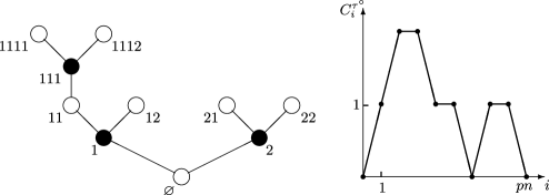
Figure 1: A $3$-tree $\tau$ and the associated contour function $C^{\tau^{\circ}}$ of $\tau^{\circ}$.

A labeled $p$-tree is a pair $\theta=(\tau,(\ell_{v})_{v\in\tau^{\circ}})$ that consists of a $p$-tree $\tau$ and a collection of integer labels assigned to the white vertices of $\tau$, such that the following properties hold: [(a)]

$\ell_{\varnothing}=0$ and $\ell_{v}\in\mathbb{Z}$ for each $v\in\tau^{\circ}$.

Let $v\in\tau^{\bullet}$, let $v_{(0)}$ be the parent of $v$ and let $v_{(j)}=vj$, $1\leq j\leq p-1$, be the children of $v$. Then for every $j\in\{0,1,\ldots,p-1\}$, $\ell_{v_{(j+1)}}\geq\ell_{v_{(j)}}-1$, where by convention $v_{(p)}=v_{(0)}$.

Condition (b) means that if one lists the white vertices adjacent to a given black vertex in clockwise order, the labels of these vertices can decrease by at most one at each step. By definition, the size of $\theta$ is the size of $\tau$.

Let $\tau$ be a $p$-tree with $n$ black vertices and let $k=\#\tau-1=pn$. The depth-first search sequence of $\tau$ is the sequence $w_{0},w_{1},\ldots,w_{2k}$ of vertices of $\tau$ which is obtained by induction as follows. First $w_{0}=\varnothing$, and then for every $i\in\{0,\ldots,2k-1\}$, $w_{i+1}$ is either the first child of $w_{i}$ that has not yet appeared in the sequence $w_{0},\ldots,w_{i}$ or the parent of $w_{i}$ if all children of $w_{i}$ already appear in the sequence $w_{0},\ldots,w_{i}$. It is easy to verify that $w_{2k}=\varnothing$ and that all vertices of $\tau$ appear in the sequence $w_{0},w_{1},\ldots,w_{2k}$ (some of them appear more than once).

Vertices $w_{i}$ are white when $i$ is even and black when $i$ is odd. The contour sequence of $\tau^{\circ}$ is by definition the sequence $v_{0},\ldots,v_{k}$ defined by $v_{i}=w_{2i}$ for every $i\in\{0,1,\ldots,k\}$. If $v$ is a given white vertex, each index $i$ such that $v_{i}=v$ corresponds to a “corner” (angular sector) around $v$, and we abusively speak about the corner $v_{i}$.

Our limit theorems for random planar maps will be derived from similar limit theorems for trees, which are conveniently stated in terms of the coding functions called the contour function and the label function. The contour function of $\tau^{\circ}$ is the discrete sequence $C^{\tau^{\circ}}_{0},C^{\tau^{\circ}}_{1},\ldots,C^{\tau^{\circ}}_{pn}$ defined by

$$C^{\tau^{\circ}}_{i}=\tfrac{1}{2}|v_{i}|\qquad\mbox{for every }0\leq i\leq pn.$$

See Figure 1 for an example with $p=n=3$. The label function of $\theta=(\tau,(\ell_{v})_{v\in\tau^{\circ}})$ is the discrete sequence $(\Lambda^{\theta}_{0},\Lambda^{\theta}_{1},\ldots,\Lambda^{\theta}_{pn})$ defined by

$$\Lambda^{\theta}_{i}=\ell_{v_{i}}\qquad\mbox{for every }0\leq i\leq pn.$$

From property (b) of the labels and the definition of the contour sequence, it is clear that $\Lambda^{\theta}_{i+1}\geq\Lambda^{\theta}_{i}-1$ for every $0\leq i\leq pn-1$. The pair $(C^{\tau^{\circ}},\Lambda^{\theta})$ determines $\theta$ uniquely.

We will need to consider subtrees of a $p$-tree $\tau$ branching from the ancestral line of a given white vertex. Let $v\in\tau^{\circ}$, and write $v=v_{j}$ for some $j\in\{0,1,\ldots,pn\}$ (the choice of $j$ does not matter in what follows). The vertices $v_{i}$, $j<i\leq pn$ which are not descendants of $v$ are partitioned into “subtrees” that can be described as follows. First, for every white vertex $u$ that is an ancestor of $v$ distinct of $v$, we can consider the subtree consisting of $u$ and of its descendants that belong to the right side of the ancestral line of $v$ (or, equivalently, that are greater than $v$ in lexicographical order). Second, for every black vertex $w$ that is an ancestor of $v$, and every child $u$ of $w$ that is greater than $v$ in lexicographical order, we can consider the subtree consisting of all descendants of $u$ (including $u$ itself). In both cases, this subtree is called a subtree branching from the right side of the ancestral line of $v$, and the quantity $\frac{1}{2}|u|$ is called the branching level of the subtree. These subtrees can be viewed as $p$-trees, modulo an obvious renaming of the vertices that preserves the lexicographical order. In the same way, we can partition the vertices $v_{i}$, $0\leq i\leq j$ which are not descendants of $v$ into subtrees branching from the left side of the ancestral line of $v$.

If we start from a labeled $p$-tree $\theta=(\tau,(\ell_{v})_{v\in\tau^{\circ}})$, we can assign labels to the white vertices of each subtree in such a way that it becomes a labeled $p$-tree: just subtract the label $\ell_{u}$ of the root $u$ of the subtree from the label of every vertex in the subtree.

2.2 The Bouttier–Di Francesco–Guitter bijection

Let $\mathbb{T}^{p}_{n}$ stand for the set of all labeled $p$-trees with $n$ black vertices. We denote the set of all rooted and pointed $2p$-angulations with $n$ faces by ${\mathcal{M}}^{p}_{n}$. An element of ${\mathcal{M}}^{p}_{n}$ is thus a pair $(M,v)$ consisting of a rooted $2p$-angulation $M\in{\mathcal{A}}^{2p}_{n}$ and a distinguished vertex $v$. By Euler’s formula, the number of choices for $v$ is $(p-1)n+2$, independently of $M$.

We now describe the Bouttier–Di Francesco–Guitter bijection (in short, the BDG bijection) between $\mathbb{T}^{p}_{n}\times\{0,1\}$ and ${\mathcal{M}}^{p}_{n}$. This bijection can be found in Section 2 of BDG in the more general setting of bipartite planar maps. Note that BDG deals with pointed planar maps rather than with rooted and pointed planar maps. However, the results described below easily follow from BDG (the bijection we will use is a variant of the one presented in IM , AM , which was concerned with nonpointed rooted $2p$-angulations and particular labeled $p$-trees called mobiles in IM , AM ).

Let $\theta=(\tau,(\ell_{v})_{v\in\tau^{\circ}})\in\mathbb{T}^{p}_{n}$ and let $\varepsilon\in\{0,1\}$. As previously, we denote the contour sequence of $\tau^{\circ}$ by $v_{0},v_{1},\ldots,v_{pn}$. We extend this sequence periodically by putting $v_{pn+i}=v_{i}$ for every $0\leq i\leq pn$. Suppose that the tree $\tau$ is drawn on the sphere and add an extra vertex $\partial$. We associate with the pair $(\theta,\varepsilon)$ a $2p$-angulation $M$ with $n$ faces, whose set of vertices is

$$\mathbf{m}=\tau^{\circ}\cup\{\partial\}$$

and whose edges are obtained as follows: For every $i\in\{0,1,\ldots,pn-1\}$,

• if $\ell_{v_{i}}=\min\{\ell_{v}\dvtx v\in\tau^{\circ}\}$, draw an edge between the corner $v_{i}$ and $\partial$;

• if $\ell_{v_{i}}>\min\{\ell_{v}\dvtx v\in\tau^{\circ}\}$, draw an edge between the corner $v_{i}$ and the corner $v_{j}$, where $j$ is the first index in the sequence $i+1,i+2,\ldots,i+pn-1$ such that $\ell_{v_{j}}=\ell_{v_{i}}-1$ (we then say that $j$ is the successor of $i$, or sometimes that $v_{j}$ is a successor of $v_{i}$).

Notice that condition (b) in the definition of a $p$-tree entails that $\ell_{v_{i+1}}\geq\ell_{v_{i}}-1$ for every $i\in\{0,1,\ldots,pn-1\}$. This ensures that whenever $\ell_{v_{i}}>\min\{\ell_{v}\dvtx v\in\tau^{\circ}\}$ there is at least one vertex among $v_{i+1},v_{i+2},\ldots,v_{i+pn-1}$ with label $\ell_{v_{i}}-1$. The construction can be made in a unique way (up to orientation-preserving homeomorphisms of the sphere) if we impose that edges of the map do not intersect, except possibly at their endpoints, and do not intersect the edges of the tree. We refer to Section 2 of BDG for a more detailed description (here we will only need the fact that edges are generated in the way described above). The resulting planar map $M$ is a $2p$-angulation. By definition, this $2p$-angulation is rooted at the edge between vertex $\varnothing$ and its successor $w=v_{j}$, where $j=\min\{i\in\{1,\ldots,pn\}\dvtx\ell_{i}=-1\}$, and by convention $w=\partial$ if $\min\{\ell_{v}\dvtx v\in\tau^{\circ}\}=0$. The orientation of this edge is specified by the variable $\varepsilon$: if $\varepsilon=1$, the root vertex is $\varnothing$ and if $\varepsilon=0$, the root vertex is $w$. Finally, the $2p$-angulation $M$ is pointed at the vertex $\partial$, so that we have indeed obtained a rooted and pointed $2p$-angulation. Each face of $M$ contains exactly one black vertex of $\tau$ (see Figure 2).

Figure 2: A labeled $3$-tree $\theta$ with $5$ black vertices and the associated $6$-angulation.

The preceding construction yields a bijection from the set $\mathbb{T}^{p}_{n}\times\{0,1\}$ onto ${\mathcal{M}}^{p}_{n}$, which is called the BDG bijection. Figure 2 gives an example of a labeled $3$-tree with $5$ black vertices (the numbers appearing inside the circles representing white vertices are the labels assigned to these vertices) and shows the $6$-angulation with $5$ faces associated with this $3$-tree via the BDG bijection.

The following property, which relates labels on the tree $\tau^{\circ}$ to distances in the planar map $M$, plays a key role. As previously, we write $d_{\mathrm{gr}}$ for the graph distance in the vertex set $\mathbf{m}$. Then, for every vertex $v\in\tau^{\circ}$, we have

$$d_{\mathrm{gr}}(\partial,v)=\ell_{v}-\min\bigl{\{}\ell_{w}\dvtx w\in\tau^{\circ}\bigr{\}}+1.$$ (3)

If $v$ and $v^{\prime}$ are two arbitrary vertices of $M$, there is no such simple expression for $d_{\mathrm{gr}}(v,v^{\prime})$ in terms of the labels on $\tau^{\circ}$. However, the following bound is useful. Suppose that $v=v_{i}$ and $v^{\prime}=v_{j}$ for some $i,j\in\{1,\ldots,pn\}$ with $i<j$. Then,

$$d_{\mathrm{gr}}\bigl{(}v,v^{\prime}\bigr{)}\leq\ell_{v_{i}}+\ell_{v_{j}}-2\max\Bigl{(}\min_{i\leq k\leq j}\ell_{v_{k}},\min_{j\leq k\leq i+pn}\ell_{v_{k}}\Bigr{)}+2.$$ (4)

See IM , Lemma 3.1, for a proof in a slightly different context, which is easily adapted. This proof makes use of simple geodesics, which are defined as follows. Let $v\in\tau^{\circ}$, and let $i\in\{0,1,\ldots,pn-1\}$ such that $v_{i}=v$. For every integer $k$ such that $0\leq k\leq\ell_{v}-\min\{\ell_{w}\dvtx w\in\tau^{\circ}\}$, put

$$\phi_{(i)}(k)=\min\bigl{\{}j\in\{i,i+1,\ldots,i+pn-1\}\dvtx\ell_{v_{j}}=\ell_{v}-k\bigr{\}},$$

and $\omega_{(i)}(k)=v_{\phi_{(i)}(k)}$. Then, if we also set $\omega_{(i)}(d_{\mathrm{gr}}(v,\partial))=\partial$, it easily follows from (3) that $(\omega_{(i)}(k),0\leq k\leq d_{\mathrm{gr}}(v,\partial))$ is a discrete geodesic from $v$ to $\partial$ in $M$. Such a geodesic is called a (discrete) simple geodesic.

The bound (4) then simply expresses the fact that the distance between $v_{i}$ and $v_{j}$ can be bounded by the length of the path obtained by concatenating the simple geodesics $\phi_{(i)}$ and $\phi_{(j)}$ up to their coalescence time.

2.3 The CRT

An important role in this work is played by the random real tree called the CRT, which was first introduced and studied by Aldous Al1 , Al3 . For our purposes, the CRT is conveniently viewed as the tree coded by a normalized Brownian excursion. Throughout this work, the notation $\mathbf{e}=(\mathbf{e}_{s})_{0\leq s\leq 1}$ stands for a normalized Brownian excursion (see RY , Chapter XII, for basic facts about Brownian excursion theory). Recall from Section 1 the definition of the pseudometric $d_{\mathbf{e}}$ and of the associated equivalence relation $\sim_{\mathbf{e}}$. By definition, the CRT is the quotient space ${\mathcal{T}}_{\mathbf{e}}:=[0,1]/\sim_{\mathbf{e}}$ and is equipped with the induced distance, which is still denoted by $d_{\mathbf{e}}$. It is easy to verify that the topology of ${\mathcal{T}}_{\mathbf{e}}$ coincides with the quotient topology.

Then $({\mathcal{T}}_{\mathbf{e}},d_{\mathbf{e}})$ is a random compact real tree (see Section 2.1 of AM for the definition and basic properties of compact real trees). We write $p_{\mathbf{e}}\dvtx[0,1]\longrightarrow{\mathcal{T}}_{\mathbf{e}}$ for the canonical projection. By convention, ${\mathcal{T}}_{\mathbf{e}}$ is rooted at the point $\rho:=p_{\mathbf{e}}(0)=p_{\mathbf{e}}(1)$. The ancestral line of a point $a$ of the CRT is the range of the unique (up to re-parametrization) continuous and injective path from the root to $a$. This ancestral line is denoted by $[\![\rho,a]\!]$. If $a,b\in{\mathcal{T}}_{\mathbf{e}}$, we say that $a$ is an ancestor of $b$ (or $b$ is a descendant of $a$) if $a\in[\![\rho,b]\!]$. For every $a\in{\mathcal{T}}_{\mathbf{e}}$, we can thus define the subtree of descendants of $a$. If $a,b\in{\mathcal{T}}_{\mathbf{e}}$, we write $a\wedge b$ for the unique vertex such that $[\![\rho,a]\!]\cap[\![\rho,b]\!]=[\![\rho,a\wedge b]\!]$.

We refer to Section 2.2 in AM for more information about the coding of compact real trees by continuous functions. Many properties related to the genealogy of ${\mathcal{T}}_{\mathbf{e}}$ can be expressed conveniently in terms of the coding function $\mathbf{e}$. For instance, if $s\in[0,1]$ is given, a point of the form $p_{\mathbf{e}}(t)$, $t\in[0,1]$, belongs to the ancestral line of $p_{\mathbf{e}}(s)$ if and only if

$$\mathbf{e}_{t}=\min_{s\wedge t\leq r\leq s\vee t}\mathbf{e}_{r}.$$

We will use such simple facts without further comment in what follows.

A leaf of ${\mathcal{T}}_{\mathbf{e}}$ is a vertex $a$ such that ${\mathcal{T}}_{\mathbf{e}}\setminus\{a\}$ is connected. If $t\in(0,1)$, the vertex $p_{\mathbf{e}}(t)$ is a leaf if and only if the equivalence class of $t$ for $\sim_{\mathbf{e}}$ is a singleton. The vertex $\rho=p_{\mathbf{e}}(0)=p_{\mathbf{e}}(1)$ is also a leaf. The set of all vertices of ${\mathcal{T}}_{\mathbf{e}}$ that are not leaves is called the skeleton of ${\mathcal{T}}_{\mathbf{e}}$ and denoted by $\operatorname{Sk}({\mathcal{T}}_{\mathbf{e}})$.

2.4 Brownian labels on the CRT

Brownian labels on the CRT are another crucial ingredient of our study. We consider a real-valued process $Z=(Z_{s})_{0\leq s\leq 1}$ such that, conditionally given $(\mathbf{e}_{s})_{0\leq s\leq 1}$, $Z$ is a centered Gaussian process with covariance

$$E[Z_{s}Z_{t}|\mathbf{e}]=\min_{s\wedge t\leq r\leq s\vee t}\mathbf{e}_{r}.$$

Note, in particular, that $Z_{0}=0$ and $E[(Z_{s}-Z_{t})^{2}|\mathbf{e}]=d_{\mathbf{e}}(s,t)$. One way of constructing the process $Z$ is via the theory of the Brownian snake Zu . It is easy to verify that $Z$ has a continuous modification, which is even Hölder continuous with exponent $\frac{1}{4}-\varepsilon$ for every $\varepsilon\in(0,\frac{1}{4})$. From now on, we always deal with this modification. From the invariance of the law of the Brownian excursion under time-reversal, one immediately gets that the processes $(\mathbf{e}_{s},Z_{s})_{0\leq s\leq 1}$ and $(\mathbf{e}_{1-s},Z_{1-s})_{0\leq s\leq 1}$ have the same distribution.

From the formula $E[(Z_{s}-Z_{t})^{2}|\mathbf{e}]=d_{\mathbf{e}}(s,t)$, one obtains that

$$Z_{s}=Z_{t}\qquad\mbox{for every }s,t\in[0,1]\mbox{ such that }d_{\mathbf{e}}(s,t)=0,\mbox{ a.s.}$$

Hence, we may view $Z$ as indexed by the CRT ${\mathcal{T}}_{\mathbf{e}}$, in such a way that $Z_{s}=Z_{p_{\mathbf{e}}(s)}$ for every $s\in[0,1]$. In what follows, we write indifferently $Z_{s}=Z_{a}$ if $s\in[0,1]$ and $a\in{\mathcal{T}}_{\mathbf{e}}$ are such that $a=p_{\mathbf{e}}(s)$. Using standard techniques as in the proof of the classical Kolmogorov lemma, one checks that the mapping ${\mathcal{T}}_{\mathbf{e}}\ni a\longrightarrow Z_{a}$ is a.s. Hölder continuous with exponent $\frac{1}{2}-\varepsilon$ with respect to $d_{\mathbf{e}}$, for every $\varepsilon\in(0,\frac{1}{2})$.

It is natural (and more intuitive than the presentation we just gave) to interpret $Z$ as a Brownian motion indexed by the CRT. Although the latter interpretation could be justified precisely, the approach we took is mathematically more tractable, as it avoids constructing a random process indexed by a random set. As we will see below, the pair $({\mathcal{T}}_{\mathbf{e}},(Z_{a})_{a\in{\mathcal{T}}_{\mathbf{e}}})$ is a continuous analog of a uniformly distributed labeled $p$-tree with $n$ black vertices.

Throughout this work, we will use the notation

$$\Delta=-\min_{0\leq s\leq 1}Z_{s}.$$

Detailed information about the distribution of $\Delta$ can be found in Delmas . Here we will only use the simple fact that the topological support of the law of $\Delta$ is the whole of $\mathbb{R}_{+}$. This can be verified by elementary arguments. It is known (see LGW , Proposition 2.5) that there is an almost surely unique instant $s_{*}\in(0,1)$ such that $Z_{s_{*}}=-\Delta$. We will write $a_{*}=p_{\mathbf{e}}(s_{*})$. Note that $a_{*}$ is a leaf of ${\mathcal{T}}_{\mathbf{e}}$.

We say that $t\in(0,1]$ is a left-increase time of $\mathbf{e}$, respectively of $Z$, if there exists $\varepsilon\in(0,t)$ such that $\mathbf{e}_{s}\geq\mathbf{e}_{t}$, respectively $Z_{s}\geq Z_{t}$, for every $s\in[t-\varepsilon,t]$. We similarly define the notion of a right-increase time. Note that the equivalence class of $t$ for $\sim_{\mathbf{e}}$ is a singleton if and only if $t$ is neither a left-increase time nor a right-increase time of $\mathbf{e}$. The following result is Lemma 3.2 in LGP .

Lemma 2.1

With probability one, any point $t\in[0,1]$ which is a right-increase or a left-increase time of $\mathbf{e}$ is neither a right-increase nor a left-increase time of $Z$.

We set for every $r\geq 0$,

$$S_{r}=\inf\bigl{\{}s\in[0,1]\dvtx Z_{s}=-r\bigr{\}}$$

with the usual convention $\inf\varnothing=\infty$. Note that $S_{r}<\infty$ if and only if $r\leq\Delta$. If $r\in(0,\Delta]$, then by definition $S_{r}$ is a left-increase time of $Z$, and Lemma 2.1 implies that the equivalence class of $S_{r}$ for $\sim_{\mathbf{e}}$ is a singleton, so that $p_{\mathbf{e}}(S_{r})$ is a leaf of ${\mathcal{T}}_{\mathbf{e}}$ (the latter property is also true for $r=0$).

The following lemma shows that, in some sense, labels do not vary too much between $S_{r}$ and $S_{r+\varepsilon}$ when $\varepsilon$ is small.

Lemma 2.2

There exists a constant $\beta_{0}\in(0,1)$ such that the following holds. Let $\mu,A,\kappa$ be three reals with $0<\mu<A$ and $\kappa\in(0,1)$. There exists a constant $C_{A,\mu,\kappa}$ such that, for every $r\in[\mu,A]$ and $\varepsilon\in(0,\mu/2)$,

$$P\Bigl{[}\{S_{r}\leq 1-\kappa\}\cap\Bigl{\{}\sup_{s\in[S_{r-\varepsilon},S_{r}]}Z_{s}\geq-r+\sqrt{\varepsilon}\Bigr{\}}\Bigr{]}\leq C_{A,\mu,\kappa}\varepsilon^{\beta_{0}}.$$

Our proof of Lemma 2.2 depends on certain fine properties of the Brownian snake, which are also used in the proof of another more difficult lemma (Lemma 5.1 below). For this reason, we postpone the proof of both results to the Appendix.

For every $s,t\in[0,1]$ such that $s\leq t$, we set

$$D^{\circ}(s,t)=D^{\circ}(t,s)=Z_{s}+Z_{t}-2\max\Bigl{(}\min_{r\in[s,t]}Z_{r},\min_{r\in[t,1]\cup[0,s]}Z_{r}\Bigr{)}.$$

We then set, for every $a,b\in{\mathcal{T}}_{\mathbf{e}}$,

$$D^{\circ}(a,b)=\min\bigl{\{}D^{\circ}(s,t)\dvtx s,t\in[0,1],p_{\mathbf{e}}(s)=a,p_{\mathbf{e}}(t)=b\bigr{\}}.$$

This is equivalent to the definition given in the introduction. Suppose that $D^{\circ}(a,b)=0$ for some $a,b\in{\mathcal{T}}_{\mathbf{e}}$ with $a\not=b$. Then we can find $s,t\in[0,1]$ such that $p_{\mathbf{e}}(s)=a$, $p_{\mathbf{e}}(t)=b$ and $D^{\circ}(s,t)=0$. Clearly, $s$ and $t$ must be (right or left) increase times of $Z$ and Lemma 2.1 implies that both $a$ and $b$ are leaves of ${\mathcal{T}}_{\mathbf{e}}$.

As a function on ${\mathcal{T}}_{\mathbf{e}}\times{\mathcal{T}}_{\mathbf{e}}$, $D^{\circ}$ does not satisfy the triangle inequality, but we can set, for every $a,b\in{\mathcal{T}}_{\mathbf{e}}$,

$$D^{*}(a,b)=\inf\Biggl{\{}\sum_{i=1}^{k}D^{\circ}(a_{i-1},a_{i})\Biggr{\}},$$

where the infimum is over all choices of the integer $k\geq 1$ and of $a_{0},\ldots,a_{k}\in{\mathcal{T}}_{\mathbf{e}}$ such that $a_{0}=a$ and $a_{k}=b$. Then $D^{*}$ is a pseudometric on ${\mathcal{T}}_{\mathbf{e}}$, and obviously $D^{*}\leq D^{\circ}$. It will sometimes be convenient to view $D^{*}$ as a function on $[0,1]^{2}$, by setting

$$D^{*}(s,t)=D^{*}\bigl{(}p_{\mathbf{e}}(s),p_{\mathbf{e}}(t)\bigr{)}$$

for every $s,t\in[0,1]$.

As a consequence of Theorem 3.4 in IM , the property $D^{*}(a,b)=0$ holds if and only if $D^{\circ}(a,b)=0$, for every $a,b\in{\mathcal{T}}_{\mathbf{e}}$, a.s. (to be precise, the results of IM are formulated in terms of a pair $(\overline{\mathbf{e}},\overline{Z})$ which corresponds to re-rooting the CRT at the vertex $p_{\mathbf{e}}(s_{*})$ with a minimal label—see Section 2.4 in IM —however, the preceding formulation easily follows from the results stated in IM ).

2.5 Convergence toward the Brownian map

For every integer $n\geq 1$, let $M_{n}$ be a random rooted and pointed $2p$-angulation, which is uniformly distributed over the set ${\mathcal{M}}_{n}^{p}$. We can write $M_{n}$ as the image under the BDG bijection of a pair $(\theta_{n},\varepsilon_{n})$, where $\theta_{n}=(\tau_{n},(\ell^{n}_{v})_{v\in\tau^{\circ}_{n}})$ is a random labeled $p$-tree and $\varepsilon_{n}$ is a random variable with values in $\{0,1\}$. Clearly, $\theta_{n}$ is uniformly distributed over the set $\mathbb{T}^{p}_{n}$ (and $\varepsilon_{n}$ is uniformly distributed over $\{0,1\}$). We write $v^{n}_{0},v^{n}_{1},\ldots,v^{n}_{pn}$ for the contour sequence of $\tau^{\circ}_{n}$. We denote the contour function of $\tau_{n}^{\circ}$ by $C^{n}=(C^{n}_{i})_{0\leq i\leq pn}$ and the label function of $\theta_{n}$ by $\Lambda^{n}=(\Lambda^{n}_{i})_{0\leq i\leq pn}$. We extend the definition of both $C^{n}$ and $\Lambda^{n}$ to the real interval $[0,pn]$ by linear interpolation.

Let $\mathbf{m}_{n}$ stand for the vertex set of $M_{n}$. Thanks to the BDG bijection, we have the identification

$$\mathbf{m}_{n}=\tau^{\circ}_{n}\cup\{\partial\},$$

where $\partial$ denotes the distinguished vertex of $M_{n}$. We also observe that the notation $\mathbf{m}_{n}$ is consistent with Section 1, since the random rooted $2p$-angulation $\mathbf{M}_{n}$ obtained from $M_{n}$ by “forgetting” the distinguished vertex of $M_{n}$ is uniformly distributed over ${\mathcal{A}}^{2p}_{n}$. Therefore, when proving Theorem 1.1, we may assume that the random metric space $(\mathbf{m}_{n},d_{\mathrm{gr}})$ is constructed from $M_{n}$ as explained above.

If $i,j\in\{0,1,\ldots,pn\}$, we set $d_{n}(i,j)=d_{\mathrm{gr}}(v^{n}_{i},v^{n}_{j})$. We have then $|\Lambda^{n}_{i}-\Lambda^{n}_{j}|\leq d_{n}(i,j)$ by (3) and the triangle inequality. As in IM , Section 3, we extend the definition of $d_{n}(s,t)$ to noninteger values of $(s,t)\in[0,pn]^{2}$ by setting

$${d}_{n}(s,t) = \bigl{(}s-\lfloor s\rfloor\bigr{)}\bigl{(}t-\lfloor t\rfloor\bigr{)}{d}_{n}\bigl{(}\lceil s\rceil,\lceil t\rceil\bigr{)}+\bigl{(}s-\lfloor s\rfloor\bigr{)}\bigl{(}\lceil t\rceil-t\bigr{)}{d}_{n}\bigl{(}\lceil s\rceil,\lfloor t\rfloor\bigr{)}$$

$${}+\bigl{(}\lceil s\rceil-s\bigr{)}\bigl{(}t-\lfloor t\rfloor\bigr{)}{d}_{n}\bigl{(}\lfloor s\rfloor,\lceil t\rceil\bigr{)}+\bigl{(}\lceil s\rceil-s\bigr{)}\bigl{(}\lceil t\rceil-t\bigr{)}{d}_{n}\bigl{(}\lfloor s\rfloor,\lfloor t\rfloor\bigr{)},$$

where $\lfloor t\rfloor=\max\{k\in\mathbb{Z}\dvtx k\leq t\}$ and $\lceil t\rceil=\min\{k\in\mathbb{Z}\dvtx k>t\}$.

The following theorem shows that the contour and label processes and the distance process associated with $M_{n}$ have a joint scaling limit, at least along a suitable sequence of integers converging to $\infty$. This result is closely related to IM , Theorem 3.4. To simplify notation, we set

$$\lambda_{p}=\frac{1}{2}\sqrt{\frac{p}{p-1}},\qquad\kappa_{p}=\biggl{(}\frac{9}{4p(p-1)}\biggr{)}^{1/4}.$$

Theorem 2.3

From every sequence of integers converging to $\infty$, we can extract a subsequence $(n_{k})_{k\geq 1}$ along which the following convergence in distribution of continuous processes holds:

$$\bigl{(}\lambda_{p}n^{-1/2}C^{n}_{pnt},\kappa_{p}n^{-1/4}\Lambda^{n}_{pnt},\kappa_{p}n^{-1/4}d_{n}(pns,pnt)\bigr{)}_{0\leq s\leq 1,0\leq t\leq 1}$$

(5)

$$\qquad\mathrel{\mathop{\longrightarrow}\limits_{n\to\infty}^{(d)}}\bigl{(}\mathbf{e}_{t},Z_{t},D(s,t)\bigr{)}_{0\leq s\leq 1,0\leq t\leq 1},$$

where the pair $(\mathbf{e},Z)$ is as in Section 2.4, and $(D(s,t))_{0\leq s\leq 1,0\leq t\leq 1}$ is a continuous random process such that the function $(s,t)\longrightarrow D(s,t)$ defines a pseudometric on $[0,1]^{2}$, and the following properties hold: [(a)]

$D(s,s_{*})=Z_{s}+\Delta=D^{\circ}(s,s_{*})$ for every $s\in[0,1]$;

$D(s,t)\leq D^{*}(s,t)\leq D^{\circ}(s,t)$ for every $s,t\in[0,1]$. For every $s,t\in[0,1]$, we put $s\approx t$ if $D(s,t)=0$. Then, a.s. for every $s,t\in[0,1]$, the property $s\approx t$ holds if and only if $D^{*}(s,t)=0$ or, equivalently, $D^{\circ}(p_{\mathbf{e}}(s),p_{\mathbf{e}}(t))=0$.

Finally, set $\mathbf{m}_{\infty}=[0,1]/\approx$ and equip $\mathbf{m}_{\infty}$ with the distance induced by $D$, which is still denoted by $D$. Then, along the same sequence where the convergence (2.3) holds, the random compact metric spaces

$$\bigl{(}\mathbf{m}_{n},\kappa_{p}n^{-1/4}d_{\mathrm{gr}}\bigr{)}$$

converge in distribution to $(\mathbf{m}_{\infty},D)$ in the sense of the Gromov–Hausdorff convergence.

(a) The bound $D(s,t)\leq D^{\circ}(s,t)$ is an analog of the bound (4). Since $D$ satisfies the triangle inequality, this bound immediately gives$D(s,t)\leq D^{*}(s,t)$ [and $D^{*}(s,t)\leq D^{\circ}(s,t)$ is true by definition as we already noticed]. [(b)]

The convergence of the first two components in (2.3) does not require the use of a subsequence; see MaMi .

The identity $D(s,s_{*})=Z_{s}+\Delta$ is a continuous analog of formula (3).

It is not hard to prove that equivalence classes for $\approx$ can contain at most $3$ points (see the discussion in IM , Section 3). Moreover, if $s$ and $t$ are distinct points of $[0,1)$ such that $s\approx t$, then we have either $p_{\mathbf{e}}(s)=p_{\mathbf{e}}(t)$ or $D^{\circ}(s,t)=0$, but these two properties cannot hold simultaneously by Lemma 2.1.

Proof of Theorem 2.3 Although this theorem is very close to the results of IM , it cannot be deduced immediately from that paper, because IM deals with rooted $2p$-angulations, where the associated tree is constructed by using distances from the root vertex, whereas in our setting of rooted and pointed $2p$-angulations the associated tree is obtained by considering the distances from the distinguished vertex. Still, the arguments in Section 3 of IM can be adapted to the present setting. The convergence of the first two components in (2.3) is deduced from MaMi , Theorem 8 (we should note that MaMi deals with the so-called height process, which is a variant of the contour process, and the corresponding variant of the label process, but it is easy to verify that limit theorems for the height process can be translated in terms of the contour process; see, for example, Section 1.6 in trees ). From this convergence, the tightness of the laws of the processes $(n^{-1/4}d_{n}(pns,pnt))_{0\leq s\leq 1,0\leq t\leq 1}$ is derived exactly as in IM , Proposition 3.2, or in Buzios , Section 6, in the particular case $p=2$. It follows that the convergence (2.3) holds along a suitable subsequence and, via the Skorokhod representation theorem, we may even assume that this convergence holds a.s. The other assertions of the theorem are then obtained in a straightforward way (see Section 3 of IM or Section 6 of Buzios ), with the exception of the fact that $D(s,t)=0$ implies $D^{*}(s,t)=0$. To verify the latter fact, one can reproduce the rather delicate arguments of IM , Section 4, in the present setting. Alternatively, one can use the estimates for the volume of balls proved in AM , Section 6, and follow the ideas that will be developed below in Section 6 to get a sharper comparison estimate between $D$ and $D^{*}$. We leave the details to the reader.

We will write $\mathbf{p}$ for the canonical projection from $[0,1]$ onto $\mathbf{m}_{\infty}=[0,1]/\approx$. As a consequence of the bound $D\leq D^{\circ}$, this projection is continuous when $[0,1]$ is equipped with the usual Euclidean distance. The volume measure $\operatorname{Vol}$ on $\mathbf{m}_{\infty}$ is the image of the Lebesgue measure on $[0,1]$ under the projection $\mathbf{p}$.

From the characterization of the equivalence relation $\approx$, we see that $\mathbf{m}_{\infty}$ can be viewed as well as a quotient space of ${\mathcal{T}}_{\mathbf{e}}$, for the equivalence relation $\simeq$ defined by $a\simeq b$ if and only if $D^{\circ}(a,b)=0$ (this is consistent with the presentation we gave in Section 1). We then write $\Pi$ for the canonical projection from ${\mathcal{T}}_{\mathbf{e}}$ onto $\mathbf{m}_{\infty}$ in such a way that $\mathbf{p}=\Pi\circ p_{\mathbf{e}}$. Noting that the topology on ${\mathcal{T}}_{\mathbf{e}}$ is the quotient topology and that $\mathbf{p}$ is continuous, it follows that $\Pi$ is also continuous. We set $x_{*}=\mathbf{p}(s_{*})=\Pi(a_{*})$. Note that property (a) in the theorem identifies all distances from $x_{*}$ in $\mathbf{m}_{\infty}$ in terms of the label process $Z$.

We can define $D^{*}(x,y)$ for every $x,y\in\mathbf{m}_{\infty}$, so that $D^{*}(\Pi(a),\Pi(b))=D^{*}(a,b)$ for every $a,b\in{\mathcal{T}}_{\mathbf{e}}$. Then $D^{*}$ is also a random distance on $\mathbf{m}_{\infty}$. Most of what follows is devoted to proving that $D(x,y)=D^{*}(x,y)$ for every $x,y\in\mathbf{m}_{\infty}$. If this equality holds, the limiting space in Theorem 2.3 coincides with $(\mathbf{m}_{\infty},D^{*})$ and in particular does not depend on the choice of the sequence $(n_{k})_{k\geq 1}$. The statement of Theorem 1.1 (in the bipartite case when $q=2p$ is even) follows.

Notice that we already know by property (b) of the theorem that $D\leq D^{*}$ and that an easy compactness argument shows that the topologies induced, respectively, by $D$ and by $D^{*}$ on $\mathbf{m}_{\infty}$ coincide, as it was already noted in IM . Furthermore, it is immediate from properties (a) and (b) in the theorem that

$$D^{*}(x_{*},x)=D(x_{*},x)\qquad\mbox{for every }x\in\mathbf{m}_{\infty}.$$ (6)

2.6 Geodesics in the Brownian map

If $x,y$ are points in a metric space $(E,d)$, a (continuous) geodesic from $x$ to $y$ is a path $(\omega(t),0\leq t\leq d(x,y))$ such that $\omega(0)=x$, $\omega(d(x,y))=y$ and $d(\omega(t),\omega(t^{\prime}))=t^{\prime}-t$ for every $0\leq t\leq t^{\prime}\leq d(x,y)$. The metric space $(E,d)$ is called geodesic if for any two points $x,y\in E$ there is (at least) one geodesic from $x$ to $y$.

From general results about Gromov–Hausdorff limits of geodesic spaces BBI , Theorem 7.5.1, we get that $(\mathbf{m}_{\infty},D)$ is almost surely a geodesic space. Detailed information about the geodesics in $\mathbf{m}_{\infty}$ has been obtained in AM , and we summarize the results that will be needed below.

Let $s\in[0,1]$. For every $r\in[0,D(s,s_{*})]$, we set

$$\varphi_{s}(r)=\cases{\inf\bigl{\{}t\in[s,1]\dvtx Z_{t}=Z_{s}-r\bigr{\}},&\quad$\mbox{if }\min\bigl{\{}Z_{t}\dvtx t\in[s,1]\bigr{\}}\leq Z_{s}-r,$\vspace*{2pt}\cr\inf\bigl{\{}t\in[0,s]\dvtx Z_{t}=Z_{s}-r\bigr{\}},&\quad$\mbox{otherwise.}$}$$

Since $D(s,s_{*})=Z_{s}+\Delta$, the preceding definition makes sense. For every $r\in[0,D(s,s_{*})]$, set

$$\Gamma_{s}(r)=\mathbf{p}\bigl{(}\varphi_{s}(r)\bigr{)}.$$

By construction, $D^{\circ}(\varphi_{s}(r),\varphi_{s}(r^{\prime}))=r^{\prime}-r$ for every $0\leq r\leq r^{\prime}\leq D(s,s_{*})$. On the other hand, by property (a) of Theorem 2.3, we have also

$$r^{\prime}-r = D^{\circ}\bigl{(}\varphi_{s}(r),\varphi_{s}\bigl{(}r^{\prime}\bigr{)}\bigr{)}\geq D\bigl{(}\varphi_{s}(r),\varphi_{s}\bigl{(}r^{\prime}\bigr{)}\bigr{)}$$

$$\geq D\bigl{(}s_{*},\varphi_{s}\bigl{(}r^{\prime}\bigr{)}\bigr{)}-D\bigl{(}s_{*},\varphi_{s}(r)\bigr{)}=r^{\prime}-r.$$

It follows that $\Gamma_{s}$ is a geodesic in $(\mathbf{m}_{\infty},D)$. Using property (b) of Theorem 2.3, we have then $D^{*}(\Gamma_{s}(r),\Gamma_{s}(r^{\prime}))=r^{\prime}-r$ for every $0\leq r\leq r^{\prime}\leq D(s,s_{*})$, and thus $\Gamma_{s}$ is also a geodesic in $(\mathbf{m}_{\infty},D^{*})$.

The geodesics of the form $\Gamma_{s}$ are called simple geodesics. They are indeed the continuous analogs of the discrete simple geodesics discussed at the end of Section 2.2.

The following theorem reformulates the main results of AM in our setting.

Theorem 2.4

All geodesics in $(\mathbf{m}_{\infty},D)$ from an arbitrary vertex of $\mathbf{m}_{\infty}$ to $x_{*}$ are simple geodesics, and therefore also geodesics in $(\mathbf{m}_{\infty},D^{*})$.

For the same reason that was discussed in the proof of Theorem 2.3, this result is not a mere restatement of Theorem 7.4 and Theorem 7.6 in AM . However, it can be deduced from these results along the following lines. Showing that all geodesics from an arbitrary vertex of $\mathbf{m}_{\infty}$ to $x_{*}$ are simple geodesics is easily seen to be equivalent to verifying that a geodesic ending at $x_{*}$ cannot visit the skeleton $\operatorname{Sk}({\mathcal{T}}_{\mathbf{e}})$, except possibly at its starting point. However, points of the skeleton are exactly those from which there are (at least) two distinct simple geodesics. Hence, supposing that there exists a geodesic ending at $x_{*}$ that visits the skeleton at a strictly positive time, one could construct two geodesics $\omega$ and $\omega^{\prime}$ starting from the same point and both ending at $x_{*}$ such that $\omega(t)=\omega^{\prime}(t)$ for every $t\in[0,\varepsilon]$, for some $\varepsilon>0$. By the invariance of the Brownian map under uniform re-rooting (Theorem 8.1 of AM ) and the main results of AM , this does not occur.

If $x\in\mathbf{m}_{\infty}$ is such that $\mathbf{p}^{-1}(x)$ is a singleton, Theorem 2.4 shows that there is a unique geodesic from $x$ to $x_{*}$. The particular case $x=\mathbf{p}(0)$ plays an important role in the remaining part of this work. In this case $\mathbf{p}^{-1}(x)=\{0,1\}$, a.s., but it is trivial that $\Gamma_{0}=\Gamma_{1}$, so that there is a.s. a unique geodesic from $\mathbf{p}(0)$ to $x_{*}$. To simplify notation, we will write $\Gamma=\Gamma_{0}$ for this unique geodesic. We note that we have $\varphi_{0}(r)=S_{r}$, for every $r\in[0,\Delta]$, where $S_{r}$ was introduced in Section 2.4, and, thus, $\Gamma(r)=\mathbf{p}(S_{r})$.

3 Maps with geodesic boundaries

3.1 Discrete maps with geodesic boundaries

We will now describe a variant of the BDG bijection that produces a $2p$-angulation with a boundary. We start from a labeled $p$-tree $\theta=(\tau,(\ell_{v})_{v\in\tau^{\circ}})$ with $n$ black vertices, and we set

$$\delta=-\min\bigl{\{}\ell_{v}\dvtx v\in\tau^{\circ}\bigr{\}}+1.$$

We use again the notation $v_{0},v_{1},\ldots,v_{pn}$ for the contour sequence of $\tau^{\circ}$. We write $M$ for the rooted and pointed $2p$-angulation associated with $\theta$ via the BDG bijection (we should have fixed $\varepsilon\in\{0,1\}$ to determine the orientation of the root edge, but the choice of $\varepsilon$ is irrelevant in what follows), and $d_{\mathrm{gr}}$ for the graph distance on the vertex set $\mathbf{m}$.

We then add $\delta-1$ vertices $\widetilde{v}_{1},\widetilde{v}_{2},\ldots,\widetilde{v}_{\delta-1}$ to the tree $\tau$ in the following way. If $k=k_{\varnothing}(\tau)$ is the number of children of $\varnothing$ in $\tau$, we put $\widetilde{v}_{1}=(k+1)$, $\tilde{v}_{2}=(k+1,1)$, $\tilde{v}_{3}=(k+1,1,1)$ and so on until $\widetilde{v}_{\delta-1}=(k+1,1,1,\ldots,1)$. For notational convenience, we also set $\widetilde{v}_{0}=\varnothing$ and $\widetilde{v}_{\delta}=\partial$. Then $\widetilde{\tau}:=\tau\cup\{\widetilde{v}_{1},\ldots,\widetilde{v}_{\delta-1}\}$ is again a plane tree (but no longer a $p$-tree). By convention, we put

$$\widetilde{\tau}^{\circ}=\tau^{\circ}\cup\{\widetilde{v}_{1},\ldots,\widetilde{v}_{\delta-1}\}.$$

We thus view $\widetilde{v}_{1},\ldots,\widetilde{v}_{\delta-1}$ as white vertices with labels $\ell_{\widetilde{v}_{i}}=-i$ for $i=1,\ldots,{\delta-1}$.

Now recall the construction of edges in the BDG bijection: For every $i\in\{0,1,\ldots,pn-1\}$ with $\ell_{i}>-\delta+1$, the corner $v_{i}$ is connected by an edge to the corner $v_{j}$, where $j\in\{i,i+1,\ldots,i+pn-1\}$ is the successor of $i$. Note that every corner of $\tau$ corresponds to one corner of $\widetilde{\tau}$ (the vertex $\varnothing$ has one more corner in $\widetilde{\tau}$, except in the particular case $\delta=1$). To construct the planar map with a boundary, we follow rules similar to those of the BDG bijection. We start by drawing an edge between $v_{i}$ and $\partial$, for all $i\in\{0,1,\ldots,pn-1\}$ such that $\ell_{v_{i}}=\min\ell$. Then, let $i\in\{0,1,\ldots,pn-1\}$ such that $\ell_{v_{i}}>\min\ell$. If the successor $j$ of $i$ is in $\{i+1,i+2,\ldots,pn\}$, we draw an edge between $v_{i}$ and $v_{j}$, as we did before. However, if the successor of $i$ is in $\{pn+1,\ldots,i+pn-1\}$, we instead draw an edge between $v_{i}$ and $\widetilde{v}_{-\ell_{i}+1}$ (since each new vertex $\widetilde{v}_{j}$ is assigned the label $-j$, $v_{i}$ is again connected by an edge to the next vertex of $\widetilde{\tau}$ with a smaller label). Finally, for every $i\in\{0,1,\ldots,\delta-1\}$, we also draw an edge between $\widetilde{v}_{i}$ and $\widetilde{v}_{i+1}$ (in particular, we draw an edge between $\widetilde{v}_{\delta-1}$ and $\partial$).

Figure 3: The DMGB associated with the $6$-angulation of Figure 2. In this case, $\delta=3$ and the two extra vertices $\widetilde{v}_{1}$ and $\widetilde{v}_{2}$ appear on the right of the figure. The map is bounded by the two boundary geodesics connecting the root of the tree to the vertex $\partial$.

The preceding construction gives a planar map $\widetilde{M}$ with vertex set $\widetilde{\mathbf{m}}=\widetilde{\tau}^{\circ}\cup\{\partial\}$ (see Figure 3 for an example). The planar map $\widetilde{M}$ is in general not a $2p$-angulation. Leaving aside the special case $\delta=1$, where $\widetilde{M}=M$, the map $\widetilde{M}$ can be viewed as a $2p$-angulation with a boundary. Indeed, it is not hard to verify that every face of $\widetilde{M}$ has degree $2p$ (and corresponds to one face in the planar map $M$), with the exception of one face, which has degree $2\delta$ and is bounded by the two geodesics from $\varnothing$ to $\partial$ that are defined as follows: $\gamma(0)=\widetilde{\gamma}(0)=\varnothing$, $\gamma(\delta)=\widetilde{\gamma}(\delta)=\partial$, and for every $i\in\{1,\ldots,\delta-1\}$,

$$\gamma(i) = v_{\phi(i)}\qquad\mbox{where }\phi(i)=\min\{j\geq 0\dvtx\ell_{v_{j}}=-i\},$$

$$\widetilde{\gamma}(i) = \widetilde{v}_{i}.$$

Let $\widetilde{d}_{\mathrm{gr}}$ be the graph distance on the vertex set $\widetilde{\mathbf{m}}$. The following properties are easily checked: [(iii)]

$\gamma$ and $\widetilde{\gamma}$ are two geodesics from $\varnothing$ to $\partial$ in $\widetilde{M}$, that intersect only at their initial and final points;

$d_{\mathrm{gr}}(v,v^{\prime})\leq\widetilde{d}_{\mathrm{gr}}(v,v^{\prime})$ for every $v,v^{\prime}\in\tau^{\circ}$;

$\widetilde{d}_{\mathrm{gr}}(v,\partial)=\ell_{v}+\delta$ for every $v\in\widetilde{\tau}^{\circ}$, and, in particular, $\widetilde{d}_{\mathrm{gr}}(v,\partial)=d_{\mathrm{gr}}(v,\partial)$ for every $v\in\tau^{\circ}$;

$\widetilde{d}_{\mathrm{gr}}(\varnothing,v)=d_{\mathrm{gr}}(\varnothing,v)$ for every $v\in\tau^{\circ}$. Informally, $M$ can be recovered from $\widetilde{M}$ by gluing the two geodesics $\gamma$ and $\widetilde{\gamma}$ onto each other (and, in particular, identifying $v_{\phi(i)}$ with $\widetilde{v}_{i}$ for every $i=1,\ldots,\delta-1$). This explains why distances from $\varnothing$ or from $\partial$ are the same in $M$ and in $\widetilde{M}$, whereas other distances may be different. Note that the geodesic $\gamma$ coincides with the discrete simple geodesic $\omega_{(0)}$ introduced at the end of Section 2.2.

We will say that $\widetilde{M}$ is the discrete map with geodesic boundaries (in short, the DMGB) associated with $M$. Notice that the boundary of $\widetilde{M}$ is only piecewise geodesic since it consists of the union of two geodesics from $\varnothing$ to $\partial$. We sometimes say that $\gamma$, respectively $\gamma^{\prime}$, is the left boundary geodesic, respectively the right boundary geodesic, of $\widetilde{M}$.

The definition of discrete simple geodesics can be extended to $\widetilde{M}$ in the following way. Recall the notation at the end of Section 2.2, and let $i\in\{0,\ldots,pn-1\}$. If the minimal label on $\tau^{\circ}$ is attained at $v_{j}$ for some $j\in\{i,\ldots,pn\}$, we just put $\widetilde{\omega}_{(i)}=\omega_{(i)}$, which is also a geodesic from $v_{i}$ to $\partial$ in $\widetilde{M}$. On the other hand, if the preceding property does not hold, there is a unique integer $k\in\{1,\ldots,d_{\mathrm{gr}}(v_{i},\partial)-1\}$ such that $\phi_{(i)}(k-1)\leq pn$ and $\phi_{(i)}(k)>pn$. Then the edge of $M$ between $\omega_{(i)}(k-1)$ and $\omega_{(i)}(k)$ does not exist in $\widetilde{M}$, but instead there is an edge of $\widetilde{M}$ between $\omega_{(i)}(k-1)$ and $\widetilde{v}_{k^{\prime}}$, where $k^{\prime}=k-\ell_{v_{i}}$. So we can put $\widetilde{\omega}_{(i)}(j)=\omega_{(i)}(j)$ if $j\leq k-1$ and $\widetilde{\omega}_{(i)}(j)=\widetilde{\gamma}(j-\ell_{v_{i}})$ if $k\leq j\leq d_{\mathrm{gr}}(v_{i},\partial)$, and $\widetilde{\omega}_{(i)}$ is again a geodesic from $v_{i}$ to $\partial$ in $\widetilde{M}$.

3.2 Scaling limits

We now apply the construction of the preceding subsection to a random $2p$-angulation $M_{n}$ that is uniformly distributed over the set ${\mathcal{M}}_{n}^{p}$. We let $\theta_{n}=(\tau_{n},(\ell^{n}_{v})_{v\in\tau_{n}})$ be the labeled $p$-tree associated with $M_{n}$, and we write $v^{n}_{0},\ldots,v^{n}_{pn}$ for the contour sequence of $\tau^{\circ}_{n}$. As previously, we also write $(C^{n}_{i})_{0\leq i\leq pn}$ for the contour function of $\tau^{\circ}_{n}$ and $(\Lambda^{n}_{i})_{0\leq i\leq pn}$ for the label function of $\theta_{n}$.

The DMGB associated with $M_{n}$ is denoted by $\widetilde{M}_{n}$. We also let $\mathbf{m}_{n}$ and $\widetilde{\mathbf{m}}_{n}$ denote, respectively, the vertex set of $M_{n}$ and the vertex set of $\widetilde{M}_{n}$.

Recall the definition of the function $d_{n}$ before Theorem 2.3. For every $i,j\in\{0,1,\ldots,pn\}$, we also set

$$\widetilde{d}_{n}(i,j)=\widetilde{d}_{\mathrm{gr}}\bigl{(}v^{n}_{i},v^{n}_{j}\bigr{)}.$$

A simple adaptation of the proof of (4) gives the bound

$$d_{n}(i,j)\leq\widetilde{d}_{n}(i,j)\leq d_{n}^{\bullet}(i,j),$$

where, for every $i,j\in\{0,1,\ldots,pn\}$,

$$d_{n}^{\bullet}(i,j)=\Lambda^{n}_{i}+\Lambda^{n}_{j}-2\min_{i\wedge j\leq k\leq i\vee j}\Lambda^{n}_{k}+2.$$

Similarly as in the case of $d_{n}$, we extend the definition of $\widetilde{d}_{n}$ to $[0,pn]\times[0,pn]$ by linear interpolation. The next proposition reinforces the joint convergence (2.3) in Theorem 2.3 by considering also the distance $\widetilde{d}_{n}$ jointly with the contour and label processes and the distance $d_{n}$.

Proposition 3.1

From every sequence of integers converging to $\infty$, we can extract a subsequence $(n_{k})_{k\geq 1}$ along which the following convergence in distribution of continuous processes indexed by $s,t\in[0,1]$ holds:

$$\bigl{(}\lambda_{p}n^{-1/2}C^{n}_{pnt},\kappa_{p}n^{-1/4}\Lambda^{n}_{pnt},\kappa_{p}n^{-1/4}d_{n}(pns,pnt),\kappa_{p}n^{-1/4}\widetilde{d}_{n}(pns,pnt)\bigr{)}$$

$$\qquad\mathrel{\mathop{\longrightarrow}\limits_{n\to\infty}^{(d)}}\bigl{(}\mathbf{e}_{t},Z_{t},D(s,t),\widetilde{D}(s,t)\bigr{)},$$

where $(\mathbf{e}_{t})_{0\leq t\leq 1}$, $(Z_{t})_{0\leq t\leq 1}$ and $(D(s,t))_{0\leq s\leq 1,0\leq t\leq 1}$ are as in Theorem 2.3, and $(\widetilde{D}(s,t))_{0\leq s\leq 1,0\leq t\leq 1}$ is a continuous random process such that $D\leq\widetilde{D}$ and the function $(s,t)\longrightarrow\widetilde{D}(s,t)$ defines a pseudometric on $[0,1]^{2}$. We put $s\equiv t$ if and only if $\widetilde{D}(s,t)=0$. The property $s\equiv t$ holds if and only if at least one of the following two conditions holds: [(a)]

$s\sim_{\mathbf{e}}t$;

$Z_{s}=Z_{t}=\min_{r\in[s\wedge t,s\vee t]}Z_{r}$. Finally, along the same sequence where the convergence (3.1) holds, we have the joint convergence in distribution of random metric spaces in the Gromov–Hausdorff sense:

$$\bigl{(}\bigl{(}\mathbf{m}_{n},\kappa_{p}n^{-1/4}d_{\mathrm{gr}}\bigr{)},\bigl{(}\widetilde{\mathbf{m}}_{n},\kappa_{p}n^{-1/4}\widetilde{d}_{\mathrm{gr}}\bigr{)}\bigr{)}\mathrel{\mathop{\longrightarrow}\limits_{n\to\infty}^{(d)}}\bigl{(}(\mathbf{m}_{\infty},D),(\widetilde{\mathbf{m}}_{\infty},\widetilde{D})\bigr{)},$$

where $(\mathbf{m}_{\infty},D)$ is as in Theorem 2.3, $\widetilde{\mathbf{m}}_{\infty}=[0,1]/\equiv$, and $\widetilde{D}$ is the induced distance on $\widetilde{\mathbf{m}}_{\infty}$.

From the bound $\widetilde{d}_{n}(i,j)\leq d_{n}^{\bullet}(i,j)$, we can use the same arguments as in the proof of IM , Proposition 3.2, to verify that the sequence of laws of the processes $(n^{-1/4}\widetilde{d}_{n}(pns,pnt))_{0\leq s,t\leq 1}$ is tight in the space of all probability measures on $C([0,1]^{2},\mathbb{R})$. To be specific, we write for every $s,t,s^{\prime},t^{\prime}\in[0,1]$,

$$\bigl{|}n^{-1/4}\widetilde{d}_{n}(pns,pnt)-n^{-1/4}\widetilde{d}_{n}\bigl{(}pns^{\prime},pnt^{\prime}\bigr{)}\bigr{|}$$

$$\qquad\leq n^{-1/4}\bigl{(}\widetilde{d}_{n}\bigl{(}pns,pns^{\prime}\bigr{)}+\widetilde{d}_{n}\bigl{(}pnt,pnt^{\prime}\bigr{)}\bigr{)}$$

$$\qquad\leq n^{-1/4}\bigl{(}d^{\bullet}_{n}\bigl{(}pns,pns^{\prime}\bigr{)}+d^{\bullet}_{n}\bigl{(}pnt,pnt^{\prime}\bigr{)}\bigr{)}.$$

By (2.3), the processes $(\kappa_{p}n^{-1/4}d^{\bullet}_{n}(pns,pnt))_{0\leq s,t\leq 1}$ converge in distribution to the process

$$\Bigl{(}Z_{s}+Z_{t}-2\min_{s\wedge t\leq r\leq s\vee t}Z_{r}\Bigr{)}_{0\leq s,t\leq 1}.$$

It then follows that, for every fixed $\delta>0$, the quantity

$$P\Bigl{(}\sup_{|s-s^{\prime}|\leq\varepsilon,|t-t^{\prime}|\leq\varepsilon}\bigl{|}n^{-1/4}\widetilde{d}_{n}(pns,pnt)-n^{-1/4}\widetilde{d}_{n}\bigl{(}pns^{\prime},pnt^{\prime}\bigr{)}\bigr{|}>\delta\Bigr{)}$$

can be made arbitrarily small, uniformly in $n$, by choosing $\varepsilon>0$ small enough. This yields the desired tightness property.

Using also the convergence (2.3), we see that we can extract a subsequence along which the convergence (3.1) holds, and obviously the processes $\mathbf{e},Z$ and $D$ satisfy the same properties as in Theorem 2.3. From now on we restrict our attention to values of $n$ in this subsequence. Using the Skorokhod representation theorem, we may assume throughout the proof that the convergence (3.1) holds a.s.

From the analogous properties for $\widetilde{d}_{n}$, it is immediate that $\widetilde{D}$ is symmetric and satisfies the triangle inequality. Note that the bound $d_{n}\leq\widetilde{d}_{n}$ implies that $D\leq\widetilde{D}$.

Let us now verify that $\widetilde{D}(s,t)=0$ if and only if (at least) one of the two conditions (a) and (b) holds. First, if (a) holds, the same argument as in the proof of Proposition 3.3(iii) in IM shows that $\widetilde{D}(s,t)=0$. Then, by passing to the limit $n\to\infty$ in the bound

$$n^{-1/4}\widetilde{d}_{n}\bigl{(}\lfloor pns\rfloor,\lfloor pnt\rfloor\bigr{)}\leq n^{-1/4}d_{n}^{\bullet}\bigl{(}\lfloor pns\rfloor,\lfloor pnt\rfloor\bigr{)},$$

we easily get that, a.s. for every $s,t\in[0,1]$,

$$\widetilde{D}(s,t)\leq Z_{s}+Z_{t}-2\min_{s\wedge t\leq r\leq s\vee t}Z_{r}.$$

If (b) holds, the right-hand side vanishes, which immediately gives $\widetilde{D}(s,t)=0$.

Conversely, suppose that $\widetilde{D}(s,t)=0$, and without loss of generality assume that $s<t$. Since $D\leq\widetilde{D}$, we have also $D(s,t)=0$ and, by Theorem 2.3, we know that either (a) holds (in which case we are done) or

$$Z_{s}=Z_{t}=\max\Bigl{(}\min_{r\in[s,t]}Z_{r},\min_{r\in[t,1]\cup[0,s]}Z_{r}\Bigr{)}.$$

If

$$Z_{s}=Z_{t}=\min_{r\in[s,t]}Z_{r},$$

then (b) holds. So we concentrate on the case where

$$Z_{s}=Z_{t}=\min_{r\in[t,1]\cup[0,s]}Z_{r}.$$ (8)

Assuming that this equality holds and that $s\sim_{\mathbf{e}}t$ does not hold, we will arrive at a contradiction, which will complete the proof of our characterization of the equivalence relation $\equiv$. We may assume that $s>0$ and $t<1$ [the case $s=0$, $t=1$ is excluded, and then we note that $\min_{[0,\varepsilon]}Z<0$ and $\min_{[1-\varepsilon,1]}Z<0$, for every $\varepsilon\in(0,1)$, a.s. by Lemma 2.1]. Then we can find positive integers $i_{n},j_{n}\in\{0,1,\ldots,pn\}$, with $i_{n}\leq j_{n}$, such that $s=\lim(pn)^{-1}i_{n}$ and $t=\lim(pn)^{-1}j_{n}$, and we have

$$\lim_{n\to\infty}\kappa_{p}n^{-1/4}\widetilde{d}_{\mathrm{gr}}\bigl{(}v^{n}_{i_{n}},v^{n}_{j_{n}}\bigr{)}=\widetilde{D}(s,t)=0.$$ (9)

From (8) and the fact that the minimum of $Z$ is attained at a unique time, we know that, for $n$ large, the minimum of $\ell^{n}$ will be attained (only) in $\{i_{n},\ldots,j_{n}\}$. Let $k_{n}\in\{i_{n},\ldots,j_{n}\}$ be the largest integer such that $\ell^{n}_{v^{n}_{k_{n}}}=\min\ell^{n}$, and write $[\![\varnothing,v^{n}_{k_{n}}]\!]$ for the ancestral line of $v^{n}_{k_{n}}$ in $\tau_{n}$. By construction, if an edge of $\widetilde{\mathbf{m}}_{n}$ connects a point of $\{v^{n}_{k_{n}},v^{n}_{k_{n}+1},\ldots,v^{n}_{pn})$ to a point of $\{v^{n}_{0},v^{n}_{1},\ldots,v^{n}_{k_{n}}\}$, then (at least) one of these two points must belong to $[\![\varnothing,v^{n}_{k_{n}}]\!]$. Therefore, if $\omega_{n}$ is a geodesic path from $v^{n}_{i_{n}}$ to $v^{n}_{j_{n}}$ in $\widetilde{\mathbf{m}}_{n}$, it must either visit $\partial$ or intersect $[\![\varnothing,v^{n}_{k_{n}}]\!]$ at (at least) one point, which may be written in the form $v^{n}_{\ell_{n}}$ with $\ell_{n}\in\{0,1,\ldots,pn\}$. The case when $\omega_{n}$ visits $\partial$ does not occur when $n$ is large, since this would imply that $Z_{s}=Z_{t}=\min Z$, which is absurd. In the other case, we can find a subsequence of the sequence $(pn)^{-1}\ell_{n}$ that converges to $r\in[0,1]$, and automatically $p_{\mathbf{e}}(r)$ belongs to the ancestral line of the vertex $a_{*}=p_{\mathbf{e}}(s_{*})$ minimizing $Z$. Furthermore, it is also clear from (9) that $\widetilde{D}(s,r)=\widetilde{D}(t,r)=0$ and, therefore, $D(s,r)=D(t,r)=0$. By Theorem 2.3, we must have $D^{\circ}(p_{\mathbf{e}}(s),p_{\mathbf{e}}(r))=0$. However, $p_{\mathbf{e}}(s)$ is a leaf of ${\mathcal{T}}_{\mathbf{e}}$ (by Lemma 2.1), whereas $p_{\mathbf{e}}(r)$ is a point of $\operatorname{Sk}({\mathcal{T}}_{\mathbf{e}})$. This contradicts our previous observation that, if $a,b\in{\mathcal{T}}_{\mathbf{e}}$ with $a\not=b$, $D^{\circ}(a,b)=0$ may hold only if $a$ and $b$ are both leaves of ${\mathcal{T}}_{\mathbf{e}}$. This contradiction completes the proof of the characterization of the property $\widetilde{D}(s,t)=0$.

We still have to prove the last convergence of the proposition. The almost sure convergence of the random compact metric spaces $(\mathbf{m}_{n},\kappa_{p}n^{-1/4}d_{\mathrm{gr}})$ toward $(\mathbf{m}_{\infty},D)$ is easily derived from the (almost sure) convergence (3.1) as in the first part of the proof of Theorem 3.4 in IM . A similar argument will give the almost sure convergence of $(\widetilde{\mathbf{m}}_{n},\kappa_{p}n^{-1/4}\widetilde{d}_{\mathrm{gr}})$ toward $(\widetilde{\mathbf{m}}_{\infty},\widetilde{D})$. Let us provide details for the sake of completeness. We first observe that we may discard the extra vertices that we added to $\mathbf{m}_{n}$ in order to define $\widetilde{\mathbf{m}}_{n}$. Indeed, it is immediate that the Hausdorff distance between $\mathbf{m}_{n}$ [viewed as a compact subset of the metric space $(\widetilde{\mathbf{m}}_{n},\widetilde{d}_{\mathrm{gr}})$] and $\widetilde{\mathbf{m}}_{n}$ is bounded by $1$, and so the Gromov–Hausdorff convergence of $(\widetilde{\mathbf{m}}_{n},\kappa_{p}n^{-1/4}\widetilde{d}_{\mathrm{gr}})$ will follow from that of $(\mathbf{m}_{n},\kappa_{p}n^{-1/4}\widetilde{d}_{\mathrm{gr}})$. For the same reason, we may replace $\mathbf{m}_{n}$ by $\mathbf{m}_{n}\setminus\{\partial\}$. We then construct a correspondence between $\mathbf{m}_{n}\setminus\{\partial\}$ and $\widetilde{\mathbf{m}}_{\infty}$ by saying that, for every $i\in\{0,1,\ldots,pn\}$ and $s\in[0,1]$, the vertex $v^{n}_{i}$ is in correspondence with the equivalence class of $s$ in $\widetilde{\mathbf{m}}_{\infty}=[0,1]/\equiv$ if $|i-pns|\leq 1$. Thanks to the convergence (3.1), we can easily verify that the distortion of this convergence, when $\mathbf{m}_{n}\setminus\{\partial\}$ is equipped with the distance $\kappa_{p}n^{-1/4}\widetilde{d}_{\mathrm{gr}}$ and $\widetilde{\mathbf{m}}_{\infty}$ with $\widetilde{D}$, tends to $0$ a.s. as $n\to\infty$. This completes the proof.

Let us state some important properties of the space $(\widetilde{\mathbf{m}}_{\infty},\widetilde{D})$. In the following proposition, as well as in the remaining part of this section, we consider the processes $(\mathbf{e},Z,D,\widetilde{D})$ and the associated random metric spaces $(\mathbf{m}_{\infty},D)$ and $(\widetilde{\mathbf{m}}_{\infty},\widetilde{D})$ that arise from the convergences of the preceding proposition via the choice of a suitable subsequence. We write $\widetilde{\mathbf{p}}$ for the canonical projection from $[0,1]$ onto $\widetilde{\mathbf{m}}_{\infty}=[0,1]/\equiv$. Recall the notation

$$\Delta=-\min\bigl{\{}Z_{s}\dvtx s\in[0,1]\bigr{\}}.$$

Proposition 3.2

(i) For every $s,t\in[0,1]$,

$$\widetilde{D}(s,t)\leq Z_{s}+Z_{t}-2\min_{s\wedge t\leq r\leq s\vee t}Z_{r}.\vspace*{-6pt}$$

[(iii)]

For every $s\in[0,1]$, $\widetilde{D}(0,s)=D(0,s)$.

For every $s\in[0,1]$, $\widetilde{D}(s,s_{*})=D(s,s_{*})=Z_{s}+\Delta$.

For every $t\in[0,\Delta]$, put

$$\widetilde{\Gamma}(t) = \widetilde{\mathbf{p}}\bigl{(}\inf\bigl{\{}s\in[0,1]\dvtx Z_{s}=-t\bigr{\}}\bigr{)},$$

$$\widetilde{\Gamma}^{\prime}(t) = \widetilde{\mathbf{p}}\bigl{(}\sup\bigl{\{}s\in[0,1]\dvtx Z_{s}=-t\bigr{\}}\bigr{)}.$$

Then $\widetilde{\Gamma}$ and $\widetilde{\Gamma}^{\prime}$ are two geodesic paths from $\widetilde{\mathbf{p}}(0)$ to $\widetilde{\mathbf{p}}(s_{*})$ in $(\widetilde{\mathbf{m}}_{\infty},\widetilde{D})$, which intersect only at their initial and final points.

Property (i) was already derived in the preceding proof. Properties (ii) and (iii) follow from the analogous properties of a DMGB stated at the end of Section 3.1 by a straightforward passage to the limit. Let us verify (iv). First it is immediate that $\widetilde{\Gamma}(0)=\widetilde{\Gamma}^{\prime}(0)=\widetilde{\mathbf{p}}(0)=\widetilde{\mathbf{p}}(1)$, and $\widetilde{\Gamma}(\Delta)=\widetilde{\Gamma}^{\prime}(\Delta)=\widetilde{\mathbf{p}}(s_{*})$. Then, from (ii) or (iii), we have

$$\widetilde{D}\bigl{(}\widetilde{\mathbf{p}}(0),\widetilde{\mathbf{p}}(s_{*})\bigr{)}=\widetilde{D}(0,s_{*})=D(0,s_{*})=\Delta.$$

On the other hand, for every $0\leq t\leq t^{\prime}\leq\Delta$, (i) gives

$$\widetilde{D}\bigl{(}\widetilde{\Gamma}(t),\widetilde{\Gamma}\bigl{(}t^{\prime}\bigr{)}\bigr{)}\leq t^{\prime}-t.$$

Thanks to the triangle inequality, this implies that $\widetilde{D}(\widetilde{\Gamma}(t),\widetilde{\Gamma}(t^{\prime}))=t^{\prime}-t$ for every $0\leq t\leq t^{\prime}\leq\Delta$. The fact that $\widetilde{\Gamma}^{\prime}$ is a geodesic path is proved in a similar way. Finally, the property $\widetilde{\Gamma}(t)\not=\widetilde{\Gamma}^{\prime}(t)$ for $t\in(0,\Delta)$ follows from the characterization of the equivalence relation $\equiv$ in Proposition 3.1, using also Lemma 2.1.

We will now explain how the space $(\widetilde{\mathbf{m}}_{\infty},\widetilde{D})$ can be constructed from $(\mathbf{m}_{\infty},D)$ by “cutting” the surface $(\mathbf{m}_{\infty},D)$ along the geodesic $\Gamma$, which produces the two geodesics $\widetilde{\Gamma}$ and $\widetilde{\Gamma}^{\prime}$. Such surgery is common in the study of the geometry of surfaces, but since we are working in a singular setting we will proceed with some care.

We set

$${\mathcal{R}}_{\Gamma}=\bigl{\{}\Gamma(t)\dvtx 0<t<\Delta\bigr{\}}\subset\mathbf{m}_{\infty},$$

and write $\overline{\mathcal{R}}_{\Gamma}={\mathcal{R}}_{\Gamma}\cup\{\mathbf{p}(0),\mathbf{p}(s_{*})\}$ for the closure of ${\mathcal{R}}_{\Gamma}$. We consider a set $\mathbf{m}^{\bullet}_{\infty}$ which is obtained from $\mathbf{m}_{\infty}$ by duplicating every point of ${\mathcal{R}}_{\Gamma}$. Formally,

$$\mathbf{m}^{\bullet}_{\infty}=(\mathbf{m}_{\infty}\setminus{\mathcal{R}}_{\Gamma})\cup\bigl{\{}(x,0)\dvtx x\in{\mathcal{R}}_{\Gamma}\bigr{\}}\cup\bigl{\{}(x,1)\dvtx x\in{\mathcal{R}}_{\Gamma}\bigr{\}}.$$

We then define a topology on $\mathbf{m}^{\bullet}_{\infty}$ by the following prescriptions:

• If $x\in\mathbf{m}_{\infty}\setminus\overline{\mathcal{R}}_{\Gamma}$, a subset of $\mathbf{m}^{\bullet}_{\infty}$ is a neighborhood of $x$ in $\mathbf{m}^{\bullet}_{\infty}$ if and only if it contains a neighborhood of $x$ in $\mathbf{m}_{\infty}$.

• A subset $V$ of $\mathbf{m}^{\bullet}_{\infty}$ is a neighborhood of $\mathbf{p}(0)$, respectively of $\mathbf{p}(s_{*})$, in $\mathbf{m}^{\bullet}_{\infty}$ if and only if there exists a neighborhood $U$ of $\mathbf{p}(0)$, respectively of $\mathbf{p}(s_{*})$, in $\mathbf{m}_{\infty}$, and $\varepsilon>0$ such that

  $$V\supset\bigl{(}(U\setminus{\mathcal{R}}_{\gamma})\cup\bigl{\{}\bigl{(}\Gamma(t),1\bigr{)}\dvtx 0\leq t\leq\varepsilon\bigr{\}}\cup\bigl{\{}\bigl{(}\Gamma(t),0\bigr{)}\dvtx 0\leq t\leq\varepsilon\bigr{\}}\bigr{)},$$

  respectively,

  $$V\supset\bigl{(}(U\setminus{\mathcal{R}}_{\gamma})\cup\bigl{\{}\bigl{(}\Gamma(t),1\bigr{)}\dvtx\Delta-\varepsilon\leq t\leq\Delta\bigr{\}}\cup\bigl{\{}\bigl{(}\Gamma(t),0\bigr{)}\dvtx\Delta-\varepsilon\leq t\leq\Delta\bigr{\}}\bigr{)}.$$

• If $x\in{\mathcal{R}}_{\Gamma}$, a subset $V$ of $\mathbf{m}^{\bullet}_{\infty}$ is a neighborhood of $(x,0)$, respectively of $(x,1)$, in $\mathbf{m}^{\bullet}_{\infty}$ if and only if there exists a neighborhood $U$ of $x$ in $\mathbf{m}_{\infty}$ such that $V$ contains $U\cap\mathbf{p}([0,s_{*}])$, respectively $U\cap\mathbf{p}([s_{*},1])$.

We write $\pi$ for the obvious projection from $\mathbf{m}^{\bullet}_{\infty}$ onto $\mathbf{m}_{\infty}$, and note that $\pi$ is continuous. We define a metric $D^{\bullet}$ on $\mathbf{m}^{\bullet}_{\infty}$ by setting, for every $x,y\in\mathbf{m}^{\bullet}_{\infty}$,

$$D^{\bullet}(x,y)=\inf\bigl{\{}L(\pi\circ g)\dvtx g\in C\bigl{(}\mathbf{m}^{\bullet}_{\infty},x\to y\bigr{)}\bigr{\}},$$

where $C(\mathbf{m}_{\infty}^{\bullet},x\to y)$ stands for the set of all continuous paths $g\dvtx[0,1]\to\mathbf{m}^{\bullet}_{\infty}$ such that $g(0)=x$ and $g(1)=y$, and $L(\pi\circ g)$ denotes the length of the path $\pi\circ g$ in $(\mathbf{m}_{\infty},D)$. Informally, the paths of the form $\pi\circ g$ are those paths from $\pi(x)$ to $\pi(y)$ in $\mathbf{m}_{\infty}$ that do not cross the geodesic $\Gamma$.

Proposition 3.3

The metric spaces $(\widetilde{\mathbf{m}}_{\infty},\widetilde{D})$ and $(\mathbf{m}_{\infty}^{\bullet},D^{\bullet})$ are almost surely isometric.

This proposition is not needed in the derivation of our main result, and so we only sketch the proof. We first observe that there is an obvious bijection $h$ from $\mathbf{m}_{\infty}^{\bullet}$ onto $\widetilde{\mathbf{m}}_{\infty}$ such that, for every $t\in(0,\Delta)$,

$$h\bigl{(}\bigl{(}\Gamma(t),0\bigr{)}\bigr{)} = \widetilde{\Gamma}(t),$$

$$h\bigl{(}\bigl{(}\Gamma(t),1\bigr{)}\bigr{)} = \widetilde{\Gamma}^{\prime}(t).$$

Indeed, every $x\in\mathbf{m}_{\infty}\setminus{\mathcal{R}}_{\Gamma}$ clearly corresponds to exactly one point $y$ of $\widetilde{\mathbf{m}}_{\infty}$ and we take $h(x)=y$.

We then need to verify that $h$ is an isometry. Since $(\widetilde{\mathbf{m}}_{\infty},\widetilde{D})$ is a geodesic space (as a Gromov–Hausdorff limit of rescaled graphs), we know that, for every $z_{1},z_{2}\in\mathbf{m}_{\infty}^{\bullet}$,

$$\widetilde{D}\bigl{(}h(z_{1}),h(z_{2})\bigr{)}=\inf\bigl{\{}\widetilde{L}(\widetilde{f})\dvtx f\in C\bigl{(}\widetilde{\mathbf{m}}_{\infty},h(z_{1})\to h(z_{2})\bigr{)}\bigr{\}},$$

where $C(\widetilde{\mathbf{m}}_{\infty},h(z_{1})\to h(z_{2}))$ is the set of all continuous paths $\widetilde{f}\dvtx[0,1]\longrightarrow\widetilde{\mathbf{m}}_{\infty}$ such that $\widetilde{f}(0)=h(z_{1})$ and $\widetilde{f}(1)=h(z_{2})$, and $\widetilde{L}(\widetilde{f})$ denotes the length of $\widetilde{f}$ in $\widetilde{\mathbf{m}}_{\infty}$. It is easy to verify that $\widetilde{f}\in C(\widetilde{\mathbf{m}}_{\infty},h(z_{1})\to h(z_{2}))$ if and only if it can be written in the form $\widetilde{f}=h\circ g$, where $g\in C(\mathbf{m}_{\infty}^{\bullet},z_{1}\to z_{2})$. Moreover, we have then

$$\widetilde{L}(\widetilde{f})=L(\pi\circ g).$$ (10)

Once (10) has been established, it readily follows from the preceding formulas for $\widetilde{D}$ and $D^{\bullet}$ that we have $\widetilde{D}(h(z_{1}),h(z_{2}))=D^{\bullet}(z_{1},z_{2})$ for every $z_{1},z_{2}\in\mathbf{m}_{\infty}^{\bullet}$, so that $h$ is an isometry. We leave the details of the proof of (10) to the reader.

3.3 A technical lemma

We will now use the results of the preceding subsection to derive a technical lemma that will play an important role later in this work. Recall the notation introduced at the beginning of Section 3.2. In particular, the random $2p$-angulation $M_{n}$ is uniformly distributed over the set ${\mathcal{M}}_{n}^{p}$, and the DMGB associated with $M_{n}$ is denoted by $\widetilde{M}_{n}$. We put $\Delta_{n}=d_{\mathrm{gr}}(\varnothing,\partial)$ (where $d_{\mathrm{gr}}$ refers to the graph distance in $M_{n}$) and following the end of Section 3.1, we introduce the two distinguished geodesics from $\varnothing$ to $\partial$ in $\widetilde{M}_{n}$, which are denoted by $\gamma_{n}$ and $\gamma^{\prime}_{n}$.

Lemma 3.4

We can find two positive constants $\varepsilon$ and $\eta$ such that, for every sufficiently large integer $n$,

$$P\Bigl{[}10n^{1/4}\leq\Delta_{n}\leq 11n^{1/4},\mathop{\mathop{\min_{n^{1/4}\leq i\leq 9n^{1/4}}}}_{n^{1/4}\leq j\leq 9n^{1/4}}\widetilde{d}_{\mathrm{gr}}\bigl{(}\gamma_{n}(i),\gamma^{\prime}_{n}(j)\bigr{)}\geq\varepsilon n^{1/4}\Bigr{]}\geq\eta.$$

Lemma 3.4 is related to the fact that the (continuous) geodesics $\widetilde{\Gamma}$ and $\widetilde{\Gamma}^{\prime}$ in Proposition 3.2 do not intersect except at their initial and final points. In the discrete setting, “interior points” of the geodesics $\gamma_{n}$ and $\gamma^{\prime}_{n}$ stay at a distance of order $n^{1/4}$.

Set $\varepsilon_{k}=2^{-k}$ and $\eta_{k}=2^{-k}$ for every integer $k\geq 0$. We argue by contradiction and assume that for every $k\geq 0$ we can find an integer $n_{k}\geq k$ such that

$$P\Bigl{[}10n_{k}^{1/4}\leq\Delta_{n_{k}}\leq 11n_{k}^{1/4},\mathop{\mathop{\min_{n_{k}^{1/4}\leq i\leq 9n_{k}^{1/4}}}_{n_{k}^{1/4}\leq j\leq 9n_{k}^{1/4}}}\widetilde{d}_{\mathrm{gr}}\bigl{(}\gamma_{n_{k}}(i),\gamma^{\prime}_{n_{k}}(j)\bigr{)}\geq\varepsilon_{k}n_{k}^{1/4}\Bigr{]}<\eta_{k}.$$ (11)

From Proposition 3.1 and replacing the sequence $(n_{k})_{k\geq 0}$ by a subsequence, we may assume that the convergence (3.1) holds along the sequence $(n_{k})_{k\geq 0}$. Notice that the bound (11) remains valid after this replacement. By using the Skorokhod representation theorem, we may even assume that (3.1) holds almost surely. From now on until the end of the proof, we consider only values of $n$ belonging to the sequence $(n_{k})_{k\geq 0}$, even if this is not indicated in the notation.

We then consider the random closed subsets $K$ and $K^{\prime}$ of $[0,1]$, which are defined by

$$K = \Bigl{\{}t\in[0,1]\dvtx Z_{t}=\min_{0\leq s\leq t}Z_{s}\in[\kappa_{p},9\kappa_{p}]\Bigr{\}},$$

$$K^{\prime} = \Bigl{\{}t\in[0,1]\dvtx Z_{t}=\min_{t\leq s\leq 1}Z_{s}\in[\kappa_{p},9\kappa_{p}]\Bigr{\}}.$$

We recall that by definition, for every $n$, and $0\leq i\leq\Delta_{n}-1$,

$$\gamma_{n}(i)=v^{n}_{\phi_{n}(i)}\qquad\mbox{where }\phi_{n}(i)=\min\bigl{\{}j\geq 0\dvtx\ell^{n}_{v^{n}_{j}}=-i\bigr{\}}.$$

No similar formula holds for $\gamma^{\prime}_{n}$, but we can write, for every $1\leq i\leq\Delta_{n}$,

$$\widetilde{d}_{\mathrm{gr}}\bigl{(}\gamma^{\prime}_{n}(i),v^{n}_{\phi^{\prime}_{n}(i)}\bigr{)}=1\qquad\mbox{where }\phi^{\prime}_{n}(i)=\max\bigl{\{}j\leq pn\dvtx\ell^{n}_{v^{n}_{j}}=-i+1\bigr{\}}.$$

The latter equality easily follows from the construction of edges in the DMGB. We thus have, for every $i\in\{0,\ldots,\Delta_{n}-1\}$ and $j\in\{1,\ldots,\Delta_{n}\}$,

$$\widetilde{d}_{\mathrm{gr}}\bigl{(}\gamma_{n}(i),\gamma^{\prime}_{n}(j)\bigr{)}\leq\widetilde{d}_{\mathrm{gr}}\bigl{(}v^{n}_{\phi_{n}(i)},v^{n}_{\phi^{\prime}_{n}(j)}\bigr{)}+1=\widetilde{d}_{n}\bigl{(}\phi_{n}(i),\phi^{\prime}_{n}(j)\bigr{)}+1.$$ (12)

Recall that $\ell^{n}_{v^{n}_{j}}=\Lambda^{n}_{j}$ and that the sequence of processes $(\kappa_{p}n^{-1/4}\Lambda^{n}_{pnt})_{0\leq t\leq 1}$ converges almost surely to $(Z_{t})_{0\leq t\leq 1}$ by (3.1). Elementary arguments using the latter convergence and the definition of the functions $\phi_{n}$ and $\phi^{\prime}_{n}$ then show that, on the event $\{\Delta>10\kappa_{p}\}$,

$$\sup_{n^{1/4}\leq i\leq 9n^{1/4}}d\biggl{(}\frac{\phi_{n}(i)}{pn},K\biggr{)}\mathrel{\mathop{\longrightarrow}\limits_{n\to\infty}^{\mathrm{a.s.}}}0,\qquad\sup_{n^{1/4}\leq j\leq 9n^{1/4}}d\biggl{(}\frac{\phi^{\prime}_{n}(j)}{pn},K^{\prime}\biggr{)}\mathrel{\mathop{\longrightarrow}\limits_{n\to\infty}^{\mathrm{a.s.}}}0,$$ (13)

where $d$ refers to the usual Euclidean distance on $[0,1]$. Notice that, on the event $\{\Delta>10\kappa_{p}\}$, we have $\Delta_{n}\geq 10n^{1/4}$ for $n$ large enough, a.s., and, in particular, $\phi_{n}(i)$ and $\phi^{\prime}_{n}(j)$ are well defined for $n^{1/4}\leq i\leq 9n^{1/4}$ and $n^{1/4}\leq j\leq 9n^{1/4}$.

From (12), (13) and the convergence (3.1), we now get, on the event $\{10\kappa_{p}<\Delta<11\kappa_{p}\}$,

$$\liminf_{k\to\infty}\Bigl{(}\kappa_{p}n_{k}^{-1/4}\mathop{\mathop{\min_{n_{k}^{1/4}\leq i\leq 9n_{k}^{1/4}}}}_{n_{k}^{1/4}\leq j\leq 9n_{k}^{1/4}}\widetilde{d}_{\mathrm{gr}}\bigl{(}\gamma_{n_{k}}(i),\gamma^{\prime}_{n_{k}}(j)\bigr{)}\Bigr{)}\geq\inf_{t\in K,t^{\prime}\in K^{\prime}}\widetilde{D}\bigl{(}t,t^{\prime}\bigr{)},$$

almost surely. In particular, for every $\varepsilon>0$,

$$\liminf_{k\to\infty}P\Bigl{[}10n_{k}^{1/4}\leq\Delta_{n_{k}}\leq 11n_{k}^{1/4},\mathop{\mathop{\min_{n_{k}^{1/4}\leq j\leq 9n_{k}^{1/4}}}_{n_{k}^{1/4}\leq i\leq 9n_{k}^{1/4}}}\widetilde{d}_{\mathrm{gr}}\bigl{(}\gamma_{n_{k}}(i),\gamma^{\prime}_{n_{k}}(j)\bigr{)}\geq\varepsilon n_{k}^{1/4}\Bigr{]}$$

$$\qquad\geq P\Bigl{[}10\kappa_{p}<\Delta<11\kappa_{p},\inf_{t\in K,t^{\prime}\in K^{\prime}}\widetilde{D}\bigl{(}t,t^{\prime}\bigr{)}>\kappa_{p}^{-1}\varepsilon\Bigr{]}.$$

The characterization of the equivalence relation $\equiv$ in Proposition 3.1 shows that $\widetilde{D}(t,t^{\prime})>0$ for every $t\in K$ and $t^{\prime}\in K^{\prime}$, a.s. on the event $\{\Delta>10\kappa_{p}\}$. By compactness, we have thus

$$\inf_{t\in K,t^{\prime}\in K^{\prime}}\widetilde{D}\bigl{(}t,t^{\prime}\bigr{)}>0$$

a.s. on that event. In particular, we can fix $\varepsilon>0$ so that the right-hand side of (3.3) is (strictly) positive. This gives a contradiction with (11), and this contradiction completes the proof.

In the next section we will use a minor extension of Lemma 3.3, concerning the case when our random $p$-tree has a random number of black vertices. Let $\mu>0$ and, for every (sufficiently large) integer $n$, consider a random labeled $p$-tree $\widehat{\theta}_{n}$ whose size belongs to $[\mu^{4}n,2\mu^{4}n]$, and such that the conditional distribution of $\widehat{\theta}_{n}$ given its size is uniform. With $\widehat{\theta}_{n}$ we associate a DMGB as explained in Section 3.1, and we let $\widehat{\gamma}_{n}$ and $\widehat{\gamma}^{\prime}_{n}$ be, respectively, the left and right boundary geodesics in this map. We also denote by $\widehat{\Delta}_{n}$ the common length of these geodesics. We can apply Lemma 3.3 to $\widehat{\theta}_{n}$ after conditioning on its size, and we get, for all sufficiently large $n$,

$$P\Bigl{[}\bigl{\{}10\mu n^{1/4}\leq\widehat{\Delta}_{n}\leq 15\mu n^{1/4}\bigr{\}}$$

(15)

$$\qquad{}\cap\Bigl{\{}\mathop{\mathop{\min_{2^{1/4}\mu n^{1/4}\leq i\leq 9\mu n^{1/4}}}_{2^{1/4}\mu n^{1/4}\leq j\leq 9\mu n^{1/4}}}\widetilde{d}_{\mathrm{gr}}\bigl{(}\widehat{\gamma}_{n}(i),\widehat{\gamma}^{\prime}_{n}(j)\bigr{)}\geq\varepsilon\mu n^{1/4}\Bigr{\}}\Bigr{]}\geq\eta.$$

4 The traversal lemmas

We use the notation of Sections 3.2 and 3.3.

Lemma 4.1

We can find a constant $\alpha_{0}>0$ such that the following holds. For every $\alpha\in(0,\alpha_{0})$, for every choice of the constants $\beta_{1}$ and $\beta_{2}$ such that $15\alpha<\beta_{1}<\beta_{2}$, and for every sufficiently large integer $n$, the probability of the event

$$\bigl{\{}\beta_{1}n^{1/4}<\Delta_{n}<\beta_{2}n^{1/4}\bigr{\}}$$

$$\qquad{}\cap\biggl{\{}\widetilde{d}_{\mathrm{gr}}\bigl{(}\gamma_{n}\bigl{(}\bigl{\lfloor}\alpha n^{1/4}\bigr{\rfloor}\bigr{)},\gamma^{\prime}_{n}\bigl{(}\bigl{\lfloor}\alpha n^{1/4}\bigr{\rfloor}\bigr{)}\bigr{)}$$

$$\hskip 18.0pt\qquad=\widetilde{d}_{\mathrm{gr}}\biggl{(}\gamma_{n}\biggl{(}\biggl{\lfloor}\frac{\alpha}{3}n^{1/4}\biggr{\rfloor}\biggr{)},\gamma^{\prime}_{n}\biggl{(}\biggl{\lfloor}\frac{\alpha}{3}n^{1/4}\biggr{\rfloor}\biggr{)}\biggr{)}+2\biggl{(}\bigl{\lfloor}\alpha n^{1/4}\bigr{\rfloor}-\biggl{\lfloor}\frac{\alpha}{3}n^{1/4}\biggr{\rfloor}\biggr{)}\biggr{\}}$$

is bounded below by a positive constant independent of $n$.

We note that, provided that $\Delta_{n}\geq\lfloor\alpha n^{1/4}\rfloor$, one has

$$\widetilde{d}_{\mathrm{gr}}\biggl{(}\gamma_{n}\bigl{(}\bigl{\lfloor}\alpha n^{1/4}\bigr{\rfloor}\bigr{)},\gamma_{n}\biggl{(}\biggl{\lfloor}\frac{\alpha}{3}n^{1/4}\biggr{\rfloor}\biggr{)}\biggr{)}=\bigl{\lfloor}\alpha n^{1/4}\bigr{\rfloor}-\biggl{\lfloor}\frac{\alpha}{3}n^{1/4}\biggr{\rfloor}$$

and similarly if $\gamma_{n}$ is replaced by $\gamma^{\prime}_{n}$. Therefore, the event considered in the lemma holds if and only if $\beta_{1}n^{1/4}<\Delta_{n}<\beta_{2}n^{1/4}$ and there exists a geodesic from $\gamma_{n}(\lfloor\alpha n^{1/4}\rfloor)$ to $\gamma^{\prime}_{n}(\lfloor\alpha n^{1/4}\rfloor)$ in $\widetilde{M}_{n}$, which visits both points $\gamma_{n}(\lfloor\frac{\alpha}{3}n^{1/4}\rfloor)$ and $\gamma^{\prime}_{n}(\lfloor\frac{\alpha}{3}n^{1/4}\rfloor)$ in this order.

To simplify notation, we will write $u_{n}=v^{n}_{\lfloor pn/2\rfloor}$ in the remaining part of this section. An important role in the proof below will be played by subtrees branching from the right side of the ancestral line of $u_{n}$ (see the end of Section 2.1).

Proof of Lemma 4.1 Recall the notation $C^{n}$ for the contour function and $\Lambda^{n}$ for the label function of the labeled $p$-tree tree $\theta_{n}=(\tau_{n},(\ell^{n}_{v})_{v\in\tau^{\circ}_{n}})$. We know from (2.3) that the pair of processes $(\lambda_{p}n^{-1/2}C^{n}_{pnt},\kappa_{p}n^{-1/4}\Lambda^{n}_{pnt})_{0\leq t\leq 1}$ converges in distribution toward $(\mathbf{e}_{t},Z_{t})_{0\leq t\leq 1}$ [this convergence does not require the use of a subsequence; see remark (a) after Theorem 2.3]. We will use this convergence in distribution to get that, with a probability bounded from below when $n$ is large, the pair $(C^{n},\Lambda^{n})$ satisfies certain properties, which can then be expressed in terms of properties of the subtrees branching from the right side of the ancestral line of $u_{n}$.

We let $\varepsilon>0$ be the constant appearing in Lemma 3.4, and we put

$$A=\biggl{\lfloor}\frac{2}{\varepsilon}\biggr{\rfloor}+1.$$

We determine $\alpha_{0}$ by the condition $p\alpha_{0}^{4}A=\frac{1}{8}$. Then we fix $\alpha\in(0,\alpha_{0})$ and $\beta_{1},\beta_{2}$ such that $15\alpha<\beta_{1}<\beta_{2}$.

Let $F$ be the event where the following properties hold:

1. [(a)]

2. We have $\mathbf{e}_{1/2}>\lambda_{p}$ and $Z_{1/2}<-\kappa_{p}\alpha$. Moreover, for any vertex $a$ of ${\mathcal{T}}_{\mathbf{e}}$ that is an ancestor of $p_{\mathbf{e}}(1/2)$ in ${\mathcal{T}}_{\mathbf{e}}$ and is such that $\frac{\lambda_{p}}{2}\leq d_{\mathbf{e}}(\rho,a)\leq\lambda_{p}$, we have $3\kappa_{p}\alpha<Z_{a}<4\kappa_{p}\alpha$.

3. $\Delta=-\min\{Z_{s}\dvtx 0\leq s\leq 1\}\in(\kappa_{p}\beta_{1},\kappa_{p}\beta_{2})$.

4. For every $s$ such that either $0\leq s\leq\sup\{r\leq\frac{1}{2}\dvtx\mathbf{e}_{r}\leq\frac{\lambda_{p}}{2}\}$ or $\inf\{r\geq\frac{1}{2}\dvtx\mathbf{e}_{r}\leq\frac{\lambda_{p}}{2}\}\leq s\leq 1$, we have $Z_{s}>-\kappa_{p}\alpha/6$.

5. There exist $A$ subintervals $[s_{1},t_{1}],\ldots,[s_{A},t_{A}]$ of $[0,1]$, with $\frac{1}{2}<s_{1}<t_{1}<\cdots<s_{A}<t_{A}<1$, such that, for every $i\in\{1,\ldots,A\}$:

   1. [(d1)]

   2. $\mathbf{e}_{s_{i}}=\mathbf{e}_{t_{i}}=\min\{\mathbf{e}_{s}\dvtx\frac{1}{2}\leq s\leq t_{i}\}$, and $\mathbf{e}_{s_{i}}\in(\frac{\lambda_{p}}{2},\lambda_{p})$.

   3. $\alpha^{4}<t_{i}-s_{i}<2\alpha^{4}$.

   4. $-15\kappa_{p}\alpha<\min_{s\in[s_{i},t_{i}]}Z_{s}-Z_{s_{i}}<-10\kappa_{p}\alpha$.

Let us comment on condition (d). By (d1), the intervals $[s_{1},t_{1}],\ldots,[s_{A},t_{A}]$ correspond to excursions of the process $(\mathbf{e}_{(1/2)+s})_{0\leq s\leq 1/2}$ above its minimum process. In particular, for every $i\in\{1,\ldots,A\}$, $p_{\mathbf{e}}(s_{i})=p_{\mathbf{e}}(t_{i})$ belongs to the ancestral line of $p_{\mathbf{e}}(1/2)$. In terms of the tree ${\mathcal{T}}_{\mathbf{e}}$ coded by $\mathbf{e}$, each interval $[s_{i},t_{i}]$ can be interpreted as a subtree branching from the ancestral line of $p_{\mathbf{e}}(1/2)$ at level $\mathbf{e}_{s_{i}}$. Condition (d2) then gives bounds for the “mass” of this subtree, and condition (d3) provides bounds for the minimal relative label on this subtree.

Simple arguments show that $P(F)>0$. The conditions that do not involve the label process $Z$ are easily seen to hold with positive probability [note that our choice of $\alpha$ such that $p\alpha^{4}A<\frac{1}{8}$ makes it possible to fulfill condition (d2)]. The fact that the other conditions then also hold with positive probability requires a little more work, but we leave the details to the reader.

For every integer $n\geq 1$, we then let $F_{n}$ be the event where the following properties hold:

1. [(a^′)]

2. We have $C^{n}_{\lfloor pn/2\rfloor}=\frac{1}{2}|u_{n}|>\sqrt{n}$ and $\ell^{n}_{u_{n}}<-\alpha n^{1/4}$. Moreover, if $v$ is a vertex of $\tau_{n}^{\circ}$ that is an ancestor of $u_{n}$ and such that $\frac{1}{2}\sqrt{n}\leq\frac{1}{2}|v|\leq\sqrt{n}$, we have $3\alpha n^{1/4}<\ell^{n}_{v}<4\alpha n^{1/4}$.

3. $\Delta_{n}=1-\min\{\ell^{n}_{v}\dvtx v\in\tau_{n}^{\circ}\}\in(\beta_{1}n^{1/4},\beta_{2}n^{1/4})$.

4. For every vertex $v$ of $\tau_{n}^{\circ}$ that belongs to a subtree branching from the left side or from the right side of the ancestral line of $u_{n}$ at level (strictly) less than $\frac{1}{2}\sqrt{n}$, we have $\ell^{n}_{v}\geq-\frac{\alpha}{6}n^{1/4}$.

5. There exist at least $A$ subtrees $\tau_{n,1},\ldots,\tau_{n,A}$ branching from the right side of the ancestral line of $u_{n}$, such that, for every $i\in\{1,\ldots,A\}$:

   1. [(d1^′)]

   2. The branching level of $\tau_{n,i}$ belongs to $[\frac{1}{2}\sqrt{n},\sqrt{n}]$.

   3. $\alpha^{4}n<|\tau_{n,i}|<2\alpha^{4}n$.

   4. The minimal difference between the label of a vertex of $\tau_{n,i}$ and the label of its root belongs to $[-15\alpha n^{1/4},-10\alpha n^{1/4}]$.

In condition (d2^′), we recall that the size $|\tau_{n,i}|$ is the number of black vertices of $\tau_{n,i}$. See Figure 4 for a rough illustration of conditions (a^′), (c^′), (d^′).

Figure 4: Illustration of the proof. The geodesic from $\widetilde{\gamma}(\lfloor\alpha n^{1/4}\rfloor)$ to $\gamma(\lfloor\alpha n^{1/4}\rfloor)$ cannot visit the part of the ancestral line of $u_{n}$ between height $\frac{1}{2}\sqrt{n}$ and height $\sqrt{n}$. If it does not visit the part of the ancestral line between $0$ and $\frac{1}{2}\sqrt{n}$, it has to cross the $A$ subtrees.

The convergence in distribution of $(\lambda_{p}n^{-1/2}C^{n}_{pnt},\kappa_{p}n^{-1/4}\Lambda^{n}_{pnt})_{0\leq t\leq 1}$ toward $(\mathbf{e}_{t},Z_{t})_{0\leq t\leq 1}$ now implies that

$$\liminf_{n\to\infty}P(F_{n})\geq P(F).$$

To see this, first note that we can replace the convergence in distribution by an almost sure convergence, thanks to the Skorokhod representation theorem. Then on the event $F$, the almost sure (uniform) convergence of $(\lambda_{p}n^{-1/2}C^{n}_{pnt})_{0\leq t\leq 1}$ toward $(\mathbf{e}_{t})_{0\leq t\leq 1})$ will imply the existence of subintervals $[m_{1},n_{1}],\ldots,[m_{A},n_{A}]$ of $[pn/2,pn]$ such that properties analogous to (d1),(d2) hold for these subintervals and for the contour function $C^{n}$. From the relation between the contour function and the tree $\tau_{n}$, we then get, still on the event $F$ and for large enough $n$, the existence of subtrees satisfying the properties in (d^′). The remaining part of the argument is straightforward.

Fix $\nu>0$ such that $P(F)>\nu$. We can then find $n_{0}$ such that $P(F_{n})\geq\nu$ for every $n\geq n_{0}$. Let us fix $n\geq n_{0}$ and argue under the conditional probability $P(\cdot|F_{n})$. We can determine the choice of the subtrees $\tau_{n,1},\ldots,\tau_{n,A}$ by saying that we choose the first $A$ subtrees branching from the right side of the ancestral line of $u_{n}$ and satisfying the conditions (d1^′), (d2^′), (d3^′), and order them in lexicographical order. As mentioned in Section 2.1, we can view each $\tau_{n,i}$ as a (random) $p$-tree, via an obvious renaming of the vertices, and we can equip the vertices of this $p$-tree with labels obtained by taking the difference of the original labels (in $\theta_{n}$) with the label of the root of $\tau_{n,i}$. In this way we obtain a random labeled $p$-tree, which we denote by $\theta_{n,i}$, for every $i\in\{1,\ldots,A\}$. Let $k_{1},\ldots,k_{A}$ be integers with $\alpha^{4}n<k_{i}<2\alpha^{4}n$ for $i\in\{1,\ldots,A\}$. We claim that under the measure $P(\cdot|F_{n})$ and conditionally on the event $\{|\tau_{n,1}|=k_{1},\ldots,|\tau_{n,A}|=k_{A}\}$, the random labeled $p$-trees $\theta_{n,1},\ldots,\theta_{n,A}$ are independent, and the conditional distribution of each $\theta_{n,i}$ is uniform over labeled $p$-trees with $k_{i}$ black vertices subject to the constraint that the minimal label belongs to $[-15\alpha n^{1/4},-10\alpha n^{1/4}]$. This follows from the fact that the tree $\theta_{n}$ is uniformly distributed, and the conditions (a^′), (b^′), (c^′) do not depend on the properties of the trees $\theta_{n,i}$ [in the case of (b^′), we note that, because of (a^′) and the assumption $\alpha<\beta_{1}/15$, the minimal label in $\tau_{n}$ will certainly not be attained at a vertex of one of the subtrees $\tau_{n,i}$].

We write $\widetilde{M}_{n,i}$ for the DMGB associated with $\theta_{n,i}$, and we let $\gamma_{n,i}$ and $\gamma^{\prime}_{n,i}$ be, respectively, the left and right boundary geodesic in $\widetilde{M}_{n,i}$. Let $G_{n}$ be the intersection of $F_{n}$ with the event where

$$\mathop{\mathop{\min_{2^{1/4}\alpha n^{1/4}\leq j\leq 9\alpha n^{1/4}}}_{2^{1/4}\alpha n^{1/4}\leq k\leq 9\alpha n^{1/4}}}\widetilde{d}_{\mathrm{gr}}\bigl{(}\gamma_{n,i}(j),\gamma^{\prime}_{n,i}(k)\bigr{)}\geq\varepsilon\alpha n^{1/4}$$ (16)

for every $i\in\{1,\ldots,A\}$ [in (16), $\widetilde{d}_{\mathrm{gr}}$ obviously stands for the graph distance in $\widetilde{M}_{n,i}$]. From (3.3) and the preceding considerations, we can find $n_{1}\geq n_{0}$ such that, for every $n\geq n_{1}$, $P(G_{n})\geq\eta^{A}P(F_{n})\geq\eta^{A}\nu$. To complete the proof of Lemma 4.1, it now suffices to verify that the event considered in this lemma contains $G_{n}$.

So suppose that $G_{n}$ holds. We already know that $\Delta_{n}\in(\beta_{1}n^{1/4},\beta_{2}n^{1/4})$ by (b^′). Next consider a geodesic path $\omega_{n}$ from $\gamma^{\prime}_{n}(\lfloor\alpha n^{1/4}\rfloor)$ to $\gamma_{n}(\lfloor\alpha n^{1/4}\rfloor)$ in $\widetilde{M}_{n}$. Recall that the label of both $\gamma_{n}(\lfloor\alpha n^{1/4}\rfloor)$ and $\gamma^{\prime}_{n}(\lfloor\alpha n^{1/4}\rfloor)$ is equal to $-\lfloor\alpha n^{1/4}\rfloor$. From the trivial bound

$$\widetilde{d}_{\mathrm{gr}}\bigl{(}\gamma^{\prime}_{n}\bigl{(}\bigl{\lfloor}\alpha n^{1/4}\bigr{\rfloor}\bigr{)},\gamma^{\prime}_{n}\bigl{(}\bigl{\lfloor}\alpha n^{1/4}\bigr{\rfloor}\bigr{)}\bigr{)}\leq 2\bigl{\lfloor}\alpha n^{1/4}\bigr{\rfloor}$$

and the fact that labels correspond to distances from $\partial$ in $\widetilde{M}_{n}$ (modulo a shift by a fixed quantity), we immediately see that the path $\omega_{n}$ cannot visit a vertex whose label is positive or strictly smaller than $-2\lfloor\alpha n^{1/4}\rfloor$. To simplify notation, write $w_{n,i}$ for the (white) vertex at generation $2i$ on the ancestral line of $u_{n}$, for every $i\in\{0,1,\ldots,\frac{|u_{n}|}{2}\}$. It follows from (a^′) and the preceding considerations that $\omega_{n}$ does not visit the set $\{w_{n,i}\dvtx\frac{1}{2}\sqrt{n}\leq i\leq\sqrt{n}\}$.

We claim that $\omega_{n}$ must visit the set $H_{n}:=\{w_{n,i}\dvtx 0\leq i<\frac{1}{2}\sqrt{n}\}$. If the claim holds, the proof is easily completed. Indeed, suppose that $\omega_{n}$ visits the vertex $w\in H_{n}$. Then we can construct a geodesic path $\widehat{\omega}_{n}$, respectively $\widehat{\omega}^{\prime}_{n}$, that connects $w$ to $\gamma_{n}(\lfloor\alpha n^{1/4}\rfloor)$, respectively to $\gamma^{\prime}_{n}(\lfloor\alpha n^{1/4}\rfloor)$, and visits the point $\gamma_{n}(\lfloor\frac{\alpha}{3}n^{1/4}\rfloor)$, respectively the point $\gamma^{\prime}_{n}(\lfloor\frac{\alpha}{3}n^{1/4}\rfloor)$. To construct $\widehat{\omega}_{n}$, pick any $k\in\{0,\ldots,\lfloor pn/2\rfloor\}$ such that $v^{n}_{k}=w$ and consider the simple geodesic $\widetilde{\omega}_{(k)}$ as defined in Section 3.1. By condition (c^′), this simple geodesic will coalesce with $\gamma_{n}$ at a point of the form $\gamma_{n}(j)$ with $j<\lfloor\frac{\alpha}{3}n^{1/4}\rfloor$. Therefore, we can just let $\widehat{\omega}_{n}$ coincide with $\omega_{(k)}$ up to its hitting time of $\gamma_{n}(\lfloor\alpha n^{1/4}\rfloor)$. Similarly, to construct $\widehat{\omega}^{\prime}_{n}$, we pick any $k^{\prime}\in\{\lfloor pn/2\rfloor,\ldots,pn\}$ such that $v^{n}_{k^{\prime}}=w$. By condition (c^′) again, the simple geodesic $\widetilde{\omega}_{(k^{\prime})}$ will coalesce with $\gamma^{\prime}_{n}$ at a point of the form $\gamma^{\prime}_{n}(j)$ with $j<\lfloor\frac{\alpha}{3}n^{1/4}\rfloor$, and we let $\widehat{\omega}^{\prime}_{n}$ coincide with $\widetilde{\omega}_{(k^{\prime})}$ up to its hitting time of $\gamma^{\prime}_{n}(\lfloor\alpha n^{1/4}\rfloor)$. The concatenation of $\widehat{\omega}_{n}$ and $\widehat{\omega}^{\prime}_{n}$ gives a geodesic path from $\gamma^{\prime}_{n}(\lfloor\alpha n^{1/4}\rfloor)$ to $\gamma_{n}(\lfloor\alpha n^{1/4}\rfloor)$ that visits both $\gamma_{n}(\lfloor\frac{\alpha}{3}n^{1/4}\rfloor)$ and $\gamma^{\prime}_{n}(\lfloor\frac{\alpha}{3}n^{1/4}\rfloor)$, as desired.

It remains to verify the claim. We argue by contradiction and suppose that $\omega_{n}$ does not visit $H_{n}$. Recall that $\omega_{n}$ does not visit the set $\{w_{n,i}\dvtx\frac{1}{2}\sqrt{n}\leq i\leq\sqrt{n}\}$ either, and notice that the condition $\ell^{n}_{u_{n}}<-\alpha n^{1/4}$ ensures that $\gamma_{n}(\lfloor\alpha n^{1/4}\rfloor)$ belongs to the left side of the ancestral line of $u_{n}$. Also recall that labels along $\omega_{n}$ must remain in the range $[-2\lfloor\alpha n^{1/4}\rfloor,0]$. From these observations, the properties (a^′) and (d3^′) and the construction of edges in $\widetilde{M}_{n}$, it follows that $\omega_{n}$ must visit each of the trees $\tau_{n,A},\tau_{n,A-1},\ldots,\tau_{n,1}$ in this order before it can hit the left side of the ancestral line of $u_{n}$. Furthermore, the path $\omega_{n}$ hits $\tau_{n,A}$ for the first time at a vertex $v$ such that the following property holds: There is no occurrence of the label $\ell^{n}_{v}-1$ among vertices that appear in the part of the contour sequence of $\tau^{\circ}_{n}$ corresponding to $\tau_{n,A}$ after the last occurrence of $v$. Indeed, this property is needed for $v$ to be connected to a vertex on the right side of $\tau_{n,A}$. If we now view $v$ as a vertex of the DMGB $\widetilde{M}_{n,A}$, this means that $v$ is connected by an edge to the vertex $\gamma^{\prime}_{n,A}(k)$, where $-k+1$ is the difference between $\ell^{n}_{v}$ and the label of the root of $\tau_{n,A}$. Since $-2\lfloor\alpha n^{1/4}\rfloor\leq\ell^{n}_{v}\leq 0$, property (a^′) implies that $3\alpha n^{1/4}-p\leq k\leq 6\alpha n^{1/4}+p+1$ (notice that although the root of $\tau_{n,A}$ may not belong to the ancestral line of $u_{n}$, its label differs by at most $p$ from the label of a vertex in this ancestral line, whose generation belongs to $[\frac{1}{2}\sqrt{n},\sqrt{n}]$). We may assume that $p+1\leq\alpha n^{1/4}$ and so we get that $2\alpha n^{1/4}\leq k\leq 7\alpha n^{1/4}$. Similarly, the last vertex of $\omega_{n}$ belonging to $\tau_{n,A}$ before $\omega_{n}$ first hits $\tau_{n,A-1}$ can be written as $\gamma_{n,A}(j)$ for some $j$ such that $2\alpha n^{1/4}\leq j\leq 7\alpha n^{1/4}$. We can now use (16) to obtain that the time spent by $\omega_{n}$ between its first visit of $\tau_{n,A}$ and its first visit of $\tau_{n,A-1}$ is at least $\varepsilon\alpha n^{1/4}$. The same lower bound holds for the time between the first hitting time of $\tau_{n,i}$ and the first hitting time of $\tau_{n,i-1}$, for every $i=A,A-1,\ldots,2$. We conclude that the length of $\omega_{n}$ is bounded below by

$$A\times\varepsilon\alpha n^{1/4}>2\alpha n^{1/4}\geq\widetilde{d}_{\mathrm{gr}}\bigl{(}\gamma_{n}\bigl{(}\bigl{\lfloor}\alpha n^{1/4}\bigr{\rfloor}\bigr{)},\gamma^{\prime}_{n}\bigl{(}\bigl{\lfloor}\alpha n^{1/4}\bigr{\rfloor}\bigr{)}\bigr{)},$$

by our choice of $A$. This contradiction completes the proof.

In our applications, we will need a version of Lemma 4.1 where the roles of the root vertex and of the distinguished vertex $\partial$ of $\mathbf{m}_{n}$ are interchanged. To this end, we will rely on a symmetry property of rooted and pointed $2p$-angulations that we state in the next lemma.

Lemma 4.2

We can construct a random $2p$-angulation $M_{n}$ with two oriented edges $e_{n}$ and $e^{*}_{n}$ and two distinguished vertices $\partial_{n}$ and $\partial^{*}_{n}$, in such a way that:

1. [(ii)]

2. Both $(M_{n},e_{n},\partial_{n})$ and $(M_{n},e^{*}_{n},\partial^{*}_{n})$ are uniformly distributed over rooted and pointed $2p$-angulations with $n$ faces.

3. If $\rho_{n}$, respectively $\rho^{*}_{n}$, is the origin of $e_{n}$, respectively of $e^{*}_{n}$, we have

   $$P\bigl{(}d_{\mathrm{gr}}\bigl{(}\partial_{n},\rho^{*}_{n}\bigr{)}>p\bigr{)}\leq\frac{2}{(p-1)n},\qquad P\bigl{(}d_{\mathrm{gr}}\bigl{(}\partial^{*}_{n},\rho_{n}\bigr{)}>p\bigr{)}\leq\frac{2}{(p-1)n}.$$

We start from a uniformly distributed rooted and pointed $2p$-angulation $M_{n}$ with $n$ faces, given (as previously) as the image under the BDG bijection of a uniformly distributed labeled $p$-tree $(\tau_{n},\ell^{n}_{v})_{v\in\tau_{n}^{\circ}}$ with $n$ black vertices and an independent Bernoulli variable $\varepsilon$ with parameter $1/2$. We let $e_{n}$ be the root edge of $M_{n}$, and as previously we write $\partial$ for the distinguished vertex of $M_{n}$. We can easily equip $M_{n}$ with another distinguished oriented edge $e^{*}_{n}$ by using the following device: We choose an independent random variable $U_{n}$ uniformly distributed over $\{0,1,\ldots,pn-1\}$ and we let $e^{*}_{n}$ be the edge generated by the $U_{n}$th step of the BDG construction, oriented uniformly at random independently of $U_{n}$. In this way, and “forgetting” the distinguished vertex $\partial$, we get a triplet $(M_{n},e_{n},e^{*}_{n})$ which is uniformly distributed over $2p$-angulations with $n$ faces and two oriented edges. Note that we distinguish the first oriented edge and the second one, so that $(M_{n},e_{n},e^{*}_{n})\not=(M_{n},e^{*}_{n},e_{n})$ unless $e_{n}=e^{*}_{n}$. However, it is easy to see (from the fact that a $2p$-angulation with $n$ faces has always $pn$ edges) that the triplets $(M_{n},e_{n},e^{*}_{n})$ and $(M_{n},e^{*}_{n},e_{n})$ have the same distribution.

Let $\rho_{n}$ and $\rho^{*}_{n}$ be the respective origins of $e_{n}$ and $e^{*}_{n}$. Although $\rho^{*}_{n}$ is not uniformly distributed over the vertex set $\mathbf{m}_{n}$ of $M_{n}$, we can construct a uniformly distributed random vertex $\partial_{n}$ that will be close to $\rho^{*}_{n}$ with high probability. To do so, recall the notation $C^{n}$ for the contour function, and $v^{n}_{0},v^{n}_{1},\ldots,v^{n}_{pn}$ for the contour sequence of $\tau^{\circ}_{n}$. If $C^{n}_{U_{n}+1}\geq C^{n}_{U_{n}}$, let $\widehat{\partial}_{n}$ be equal to $v^{n}_{U_{n}+1}$. On the other hand, if $C^{n}_{U_{n}}>C^{n}_{U_{n}+1}$, we let $\widehat{\partial}_{n}$ be chosen uniformly at random among the $p-1$ children of the black vertex which is the parent of $v^{n}_{U_{n}}$ in $\tau_{n}$. Then it is not hard to see that $\widehat{\partial}_{n}$ and $\rho^{*}_{n}$ are on the boundary of the same face of $M_{n}$, so that $d_{\mathrm{gr}}(\widehat{\partial}_{n},\rho^{*}_{n})\leq p$. Furthermore, a moment’s thought shows that $\widehat{\partial}_{n}$ is uniformly distributed over $\mathbf{m}_{n}\setminus\{\varnothing,\partial\}$. So, independently of the other random quantities, we may define

$$\partial_{n}=\cases{\widehat{\partial}_{n},&\quad$\mbox{with probability }\displaystyle\frac{(p-1)n}{(p-1)n+2},$\vspace*{2pt}\cr\varnothing,&\quad$\mbox{with probability }\displaystyle\frac{1}{(p-1)n+2},$\vspace*{2pt}\cr\partial,&\quad$\mbox{with probability }\displaystyle\frac{1}{(p-1)n+2},$}$$

so that the triplet $(M_{n},e_{n},\partial_{n})$ is uniformly distributed over rooted and pointed $2p$-angulations with $n$ faces, and the first bound in (ii) holds by the preceding considerations.

To complete the proof, we select independently of $e_{n}^{*}$ and of the other random quantities a random vertex $\widetilde{\partial}_{n}$ uniformly distributed over $\mathbf{m}_{n}$. Applying the (inverse) BDG bijection to the (uniformly distributed) rooted and pointed $2p$-angulation $(M_{n},e^{*}_{n},\widetilde{\partial}_{n})$, we can associate with the edge $e_{n}$ a random variable $U^{*}_{n}$ uniformly distributed over $\{0,1,\ldots,pn-1\}$ (just as $U_{n}$ was associated with $e^{*}_{n}$). By duplicating the preceding argument, we then construct from $U^{*}_{n}$ a random vertex $\partial^{*}_{n}$ such that $(M_{n},e^{*}_{n},\partial^{*}_{n})$ is uniformly distributed and the second bound in (ii) holds.

If $\omega=(\omega(0),\omega(1),\ldots,\omega(k))$ is a path in $M_{n}$, the length of $\omega$ is $|\omega|=k$, and the reversed path $(\omega(|\omega|),\omega(|\omega|-1),\ldots,\omega(0))$ is denoted by $\overline{\omega}$. Recall the constant $\alpha_{0}$ introduced in Lemma 4.1.

Lemma 4.3

Let $\alpha\in(0,\alpha_{0})$ and $\beta_{1},\beta_{2}$ such that $15\alpha<\beta_{1}<\beta_{2}$. For every integer $n\geq 1$, and every $\delta>0$, consider the event

$${\mathcal{E}}_{n,\delta} = \bigl{\{}\beta_{1}n^{1/4}<\Delta_{n}<\beta_{2}n^{1/4}\bigr{\}}$$

$${}\cap\biggl{\{}\widetilde{d}_{\mathrm{gr}}\bigl{(}\overline{\gamma}_{n}\bigl{(}\bigl{\lfloor}\alpha n^{1/4}\bigr{\rfloor}\bigr{)},\overline{\gamma}^{\prime}_{n}\bigl{(}\bigl{\lfloor}\alpha n^{1/4}\bigr{\rfloor}\bigr{)}\bigr{)},$$

$$\hskip 18.0pt\geq\widetilde{d}_{\mathrm{gr}}\biggl{(}\overline{\gamma}_{n}\biggl{(}\biggl{\lfloor}\frac{\alpha}{3}n^{1/4}\biggr{\rfloor}\biggr{)}\overline{\gamma}^{\prime}_{n}\biggl{(}\biggl{\lfloor}\frac{\alpha}{3}n^{1/4}\biggr{\rfloor}\biggr{)}\biggr{)}+\biggl{(}\frac{4\alpha}{3}-\delta\biggr{)}n^{1/4}\biggr{\}}.$$

There exist a real sequence $(\delta_{n})_{n\geq 0}$ decreasing to $0$, and a constant $a_{1}>0$ such that

$$P({\mathcal{E}}_{n,\delta_{n}})\geq a_{1}$$

for every sufficiently large integer $n$.

Furthermore, if the event ${\mathcal{E}}_{n,\delta_{n}}$ holds, we have also

$$\widetilde{d}_{\mathrm{gr}}\bigl{(}\overline{\gamma}^{\prime}_{n}\bigl{(}j^{\prime}\bigr{)},\overline{\gamma}_{n}(j)\bigr{)}$$

(17)

$$\qquad\geq\widetilde{d}_{\mathrm{gr}}\biggl{(}\overline{\gamma}^{\prime}_{n}\bigl{(}j^{\prime}\bigr{)},\overline{\gamma}_{n}\biggl{(}\biggl{\lfloor}\frac{\alpha}{3}n^{1/4}\biggr{\rfloor}\biggr{)}\biggr{)}+j-\biggl{\lfloor}\frac{\alpha}{3}n^{1/4}\biggr{\rfloor}-\delta_{n}n^{1/4}-2$$

for every $j\in\{\lfloor\frac{\alpha}{3}n^{1/4}\rfloor,\ldots,\lfloor\alpha n^{1/4}\rfloor\}$ and $j^{\prime}\in\{0,1,\ldots,\lfloor\alpha n^{1/4}\rfloor\}$. The same bound holds if the roles of $\overline{\gamma}_{n}$ and $\overline{\gamma}^{\prime}_{n}$ are interchanged.

We start by proving the existence of a constant $a_{2}>0$ such that, for every $\delta>0$,

$$\liminf_{n\to\infty}P({\mathcal{E}}_{n,\delta})\geq a_{2}.$$ (18)

The first part of the lemma follows: Just construct by induction a monotone increasing sequence $(n_{k})_{k\geq 0}$ such that $P({\mathcal{E}}_{n,2^{-k}})\geq a_{2}/2$ for every $n\geq n_{k}$, and put $\delta_{n}=2^{-k}$ for $n_{k}\leq n<n_{k+1}$.

We consider a random $2p$-angulation $M_{n}$ with two oriented edges $e_{n}$ and $e^{*}_{n}$ and two distinguished vertices $\partial_{n}$ and $\partial^{*}_{n}$, such that properties (i) and (ii) of Lemma 4.2 hold. We also write $\rho_{n}$ and $\rho^{*}_{n}$ for the respective origins of $e_{n}$ and $e^{*}_{n}$. With the uniformly distributed rooted and pointed $2p$-angulation $(M_{n},e_{n},\partial_{n})$ we associate the DMGB $\widetilde{M}_{n}$, and similarly with $(M_{n},e^{*}_{n},\partial^{*}_{n})$ we associate the DMGB $\widetilde{M}_{n}^{*}$. We write $\gamma_{n}$ and $\gamma^{\prime}_{n}$, respectively $\gamma^{*}_{n}$ and ${\gamma^{*}_{n}}^{\prime}$, for the left and right boundary geodesics in $\widetilde{M}_{n}$, respectively in $\widetilde{M}^{*}_{n}$. The common length of $\gamma_{n}$ and $\gamma^{\prime}_{n}$, respectively of $\gamma^{*}_{n}$ and ${\gamma^{*}_{n}}^{\prime}$, is denoted by $\Delta_{n}$, respectively by $\Delta^{*}_{n}$. Notice that $\gamma_{n}$, respectively $\gamma^{*}_{n}$, can also be viewed as a geodesic in $M_{n}$, which starts from one of the two vertices incident to $e_{n}$, respectively to $e^{*}_{n}$, and ends at $\partial_{n}$, respectively at $\partial^{*}_{n}$.

Thanks to property (ii) of Lemma 4.2, we can use $\gamma_{n}^{*}$, or rather the time-reversed path $\overline{\gamma}_{n}^{*}$, to construct an “approximate” geodesic from $\rho_{n}$ to $\partial_{n}$ in $M_{n}$. To do so, we concatenate a geodesic path from $\rho_{n}$ to $\partial^{*}_{n}$ with the path $\overline{\gamma}_{n}^{*}$, and then with a geodesic path from the initial point of $\gamma^{*}_{n}$ (which is either $\rho^{*}_{n}$ or a neighbor of $\rho^{*}_{n}$) to $\partial_{n}$. Let $\gamma_{n}^{**}$ be the path resulting from this concatenation. From property (ii) of Lemma 4.2, the length of $\gamma_{n}^{**}$ is bounded above by $d_{\mathrm{gr}}(\rho_{n},\partial_{n})+4(p+1)$, with probability at least $1-2((p-1)n)^{-1}$. From Proposition 1.1 in AM (and the fact that this result also holds for approximate geodesics as discussed in the introduction of AM ), we know that the paths $\gamma_{n}$ and $\gamma_{n}^{**}$ must be close to each other with high probability when $n$ is large. More precisely, we get for every $\varepsilon>0$,

$$\lim_{n\to\infty}P\Bigl{[}\max_{i\geq 0}d_{\mathrm{gr}}\bigl{(}\gamma_{n}(i\wedge\Delta_{n}),\overline{\gamma}_{n}^{*}\bigl{(}i\wedge\Delta_{n}^{*}\bigr{)}\bigr{)}>\varepsilon n^{1/4}\Bigr{]}=0.$$ (19)

In what follows, we suppose that the event considered in Lemma 4.1 holds for the DMGB $\widetilde{M}_{n}$. We fix $\delta>0$ and using the property (19), we will show that we have on this event

$$\widetilde{d}_{\mathrm{gr}}\bigl{(}\overline{\gamma}^{*}_{n}\bigl{(}\bigl{\lfloor}\alpha n^{1/4}\bigr{\rfloor}\bigr{)},\overline{\gamma}^{*\prime}_{n}\bigl{(}\bigl{\lfloor}\alpha n^{1/4}\bigr{\rfloor}\bigr{)}\bigr{)}$$

(20)

$$\qquad\geq\widetilde{d}_{\mathrm{gr}}\biggl{(}\overline{\gamma}^{*}_{n}\biggl{(}\biggl{\lfloor}\frac{\alpha}{3}n^{1/4}\biggr{\rfloor}\biggr{)},\overline{\gamma}^{*\prime}_{n}\biggl{(}\biggl{\lfloor}\frac{\alpha}{3}n^{1/4}\biggr{\rfloor}\biggr{)}\biggr{)}+\biggl{(}\frac{4\alpha}{3}-\delta\biggr{)}n^{1/4},$$

except possibly on a set of probability tending to $0$ when $n\to\infty$. Our claim (18) will follow since the DMGBs $\widetilde{M}_{n}$ and $\widetilde{M}_{n}^{*}$ have the same distribution [and $P(|\Delta_{n}-\Delta_{n}^{*}|\geq\varepsilon n^{1/4})$ tends to $0$ as $n\to\infty$, for every $\varepsilon>0$].

Without loss of generality, we can assume that $0<\delta<\alpha/2$. We write $B_{M_{n}}(v,r)$, respectively $B_{\widetilde{M}_{n}}(v,r)$, $B_{\widetilde{M}_{n}^{*}}(v,r)$ for the open ball of radius $r$ centered at $v$ in $M_{n}$, respectively in $\widetilde{M}_{n}$, in $\widetilde{M}_{n}^{*}$. We first note that a geodesic path in $\widetilde{M}_{n}$ from $\gamma^{\prime}_{n}(\lfloor\alpha n^{1/4}\rfloor)$ to $\gamma_{n}(\lfloor\alpha n^{1/4}\rfloor)$ cannot visit $B_{\widetilde{M}_{n}}(\partial_{n},\delta n^{1/4})$, because otherwise its length would be at least $2(\Delta_{n}-\delta n^{1/4}-\lfloor\alpha n^{1/4}\rfloor)\geq 2(\beta_{1}-\delta-\alpha)n^{1/4}$, which is clearly impossible. For the same reason, a geodesic path in $\widetilde{M}_{n}^{*}$ from $\overline{\gamma}^{*\prime}_{n}(\lfloor\alpha n^{1/4}\rfloor)$ to $\overline{\gamma}^{*}_{n}(\lfloor\alpha n^{1/4}\rfloor)$ does not visit $B_{\widetilde{M}_{n}^{*}}(\gamma_{n}^{*}(0),\delta n^{1/4})$, except perhaps on a set of probability tending to $0$ as $n$ tends to infinity, which we may discard.

To simplify notation, set ${\mathcal{R}}(\gamma_{n})=\{\gamma_{n}(i)\dvtx 0\leq i\leq\Delta_{n}\}$. Let $i_{0}\in\{1,\ldots,\break\Delta_{n}-1\}$. A path $\omega=(\omega(i),0\leq i\leq|\omega|)$ in $M_{n}$ is said to be an admissible loop from $\gamma_{n}(i_{0})$ in $M_{n}$ if $\omega(0)=\omega(|\omega|)=\gamma_{n}(i_{0})$, if $\omega$ does not visit $\gamma_{n}(0)$ or $\gamma_{n}(\Delta_{n})$, and if there exist integers $k_{\omega}$ and $\ell_{\omega}$ such that $0\leq k_{\omega}<\ell_{\omega}\leq|\omega|$, and the following holds: [(iii)]

$\omega(i)\in{\mathcal{R}}(\gamma_{n})$ if and only if $0\leq i\leq k_{\omega}$ or $\ell_{\omega}\leq i\leq|\omega|$;

$\omega(k_{\omega})$ is connected to $\omega(k_{\omega}+1)$ by an edge starting from a corner belonging to the left side of $\gamma_{n}$ [here and later, $\gamma_{n}$ is oriented from $\gamma_{n}(0)$ to $\gamma_{n}(\Delta_{n})$];

$\omega(\ell_{\omega})$ is connected to $\omega(\ell_{\omega}-1)$ by an edge starting from a corner belonging to the right side of $\gamma_{n}$. In the same way, we define a $*$-admissible loop in $M_{n}$ by replacing $\gamma_{n}$ with $\overline{\gamma}^{*}_{n}$ and $\Delta_{n}$ with $\Delta_{n}^{*}$ everywhere in the previous definition. Note that an admissible loop (resp., a $*$-admissible loop) winds exactly once in clockwise order around the point $\gamma_{n}(\Delta_{n})=\partial_{n}$ [resp., around $\overline{\gamma}_{n}^{*}(\Delta_{n}^{*})=\gamma_{n}^{*}(0)$] in the twice punctured sphere ${\mathbb{S}}^{2}\setminus\{\gamma_{n}(0),\gamma_{n}(\Delta_{n})\}$ (resp., in ${\mathbb{S}}^{2}\setminus\{\gamma^{*}_{n}(0),\gamma^{*}_{n}(\Delta^{*}_{n})\}$).

The following properties are easily checked from the relation between $M_{n}$ and $\widetilde{M}_{n}$ or $\widetilde{M}^{*}_{n}$: [(a)]

If $\omega$ is an admissible loop from $\gamma_{n}(i_{0})$, then we can find a path $\widetilde{\omega}$ in $\widetilde{M}_{n}$ such that $\widetilde{\omega}(0)=\gamma^{\prime}_{n}(i_{0})$, $\widetilde{\omega}(|\widetilde{\omega}|)=\gamma_{n}(i_{0})$ and $|\widetilde{\omega}|=|\omega|$.

Similarly, if $\omega^{*}$ is a $*$-admissible loop from $\overline{\gamma}_{n}^{*}(i_{0})$, then we can find a path $\widetilde{\omega}^{*}$ in $\widetilde{M}_{n}^{*}$ such that $\widetilde{\omega}(0)=\overline{\gamma}^{*\prime}_{n}(i_{0})$, $\widetilde{\omega}(|\widetilde{\omega}|)=\overline{\gamma}_{n}^{*}(i_{0})$ and $|\widetilde{\omega}^{*}|=|\omega^{*}|$.

Let $\widetilde{\omega}$ be a path in $\widetilde{M}_{n}$ that does not visit $\gamma_{n}(0)$ or $\gamma_{n}(\Delta_{n})$, such that $\widetilde{\omega}(0)=\gamma_{n}^{\prime}(i_{0})$ and $\widetilde{\omega}(|\widetilde{\omega}|)=\gamma_{n}(i_{0})$, and such that $\widetilde{\omega}$ visits $\gamma^{\prime}_{n}(i)$ and $\gamma_{n}(i)$ in this order, for some $i\in\{1,\ldots,\Delta_{n}-1\}$. Then we can find an admissible loop $\omega$ from $\gamma_{n}(i_{0})$ such that $|\omega|\leq|\widetilde{\omega}|$, and such that $\gamma_{n}(i)\in\{\omega(j)\dvtx 0\leq j\leq k_{\omega}\}\cap\{\omega(j)\dvtx\ell_{\omega}\leq j\leq|\omega|\}$. If, for some $r,r^{\prime}>0$, $\widetilde{\omega}$ does not visit $B_{\widetilde{M}_{n}}(\gamma_{n}(0),r)\cup B_{\widetilde{M}_{n}}(\gamma_{n}(\Delta_{n}),r^{\prime})$, then $\omega$ can be constructed so that it does not visit $B_{M_{n}}(\gamma_{n}(0),r)\cup B_{M_{n}}(\gamma_{n}(\Delta_{n}),r^{\prime})$.

Similarly, if $\widetilde{\omega}^{*}$ is any path in $\widetilde{M}_{n}^{*}$ that does not visit $\overline{\gamma}_{n}(0)$ or $\overline{\gamma}_{n}(\Delta_{n}^{*})$ and is such that $\widetilde{\omega}(0)=\overline{\gamma}^{*\prime}_{n}(i_{0})$ and $\widetilde{\omega}^{*}(|\widetilde{\omega}^{*}|)={\overline{\gamma}_{n}^{*}}(i_{0})$, then we can find a $*$-admissible loop $\omega^{*}$ from $\overline{\gamma}_{n}^{*}(i_{0})$ such that $|\omega^{*}|\leq|\widetilde{\omega}^{*}|$. If, for some $r,r^{\prime}>0$, $\widetilde{\omega}^{*}$ does not visit $B_{\widetilde{M}_{n}^{*}}(\overline{\gamma}_{n}^{*}(0),r)\cup B_{\widetilde{M}_{n}^{*}}(\overline{\gamma}_{n}(\Delta_{n}^{*}),r^{\prime})$, then $\omega^{*}$ can be constructed so that it does not visit $B_{M_{n}}(\overline{\gamma}_{n}^{*}(0),r)\cup B_{M_{n}}(\overline{\gamma}_{n}(\Delta_{n}^{*}),r^{\prime})$.

Let $\widetilde{\omega}_{n}^{*}$ be a geodesic in $\widetilde{M}_{n}^{*}$ from $\overline{\gamma}^{*\prime}_{n}(\lfloor\alpha n^{1/4}\rfloor)$ to $\overline{\gamma}^{*}_{n}(\lfloor\alpha n^{1/4}\rfloor)$. As mentioned above, we may assume that $\widetilde{\omega}_{n}^{*}$ does not visit $B_{\widetilde{M}_{n}^{*}}(\gamma_{n}^{*}(0),\delta n^{1/4})$. Also, if $\widetilde{\omega}_{n}^{*}$ visits $B_{\widetilde{M}_{n}^{*}}(\partial_{n}^{*},\frac{\delta}{4}n^{1/4})$, then it readily follows that (4) holds. So we may restrict our attention to the case when $\widetilde{\omega}_{n}^{*}$ does not visit this ball.

By property (d) above, we can construct a $*$-admissible loop $\omega^{*}$ from $\overline{\gamma}_{n}^{*}(\lfloor\alpha n^{1/4}\rfloor)$, such that $|\omega^{*}|\leq\widetilde{d}_{\mathrm{gr}}(\overline{\gamma}^{*}_{n}(\lfloor\alpha n^{1/4}\rfloor),\overline{\gamma}^{*\prime}_{n}(\lfloor\alpha n^{1/4}\rfloor))$ and such that $\omega^{*}$ does not visit $B_{M_{n}}(\gamma_{n}^{*}(0),\delta n^{1/4})$ or $B_{M_{n}}(\partial_{n}^{*},\frac{\delta}{4}n^{1/4})$. Now pick a geodesic $g_{n}$ from $\gamma_{n}(\lfloor\alpha n^{1/4}\rfloor)$ to $\overline{\gamma}^{*}_{n}(\lfloor\alpha n^{1/4}\rfloor)$ and note that, thanks to (19), we have $|g_{n}|\leq\frac{\delta}{16}n^{1/4}$, except on a set of probability tending to $0$ which we may discard. By concatenating $g_{n}$, $\omega^{*}$ and the time-reversed path $\overline{g}_{n}$, we get a path $\omega$ whose length is bounded above by $|\omega^{*}|+\frac{\delta}{8}n^{1/4}$, and which starts and ends at $\gamma_{n}(\lfloor\alpha n^{1/4}\rfloor)$. Moreover, we can also use property (ii) of Lemma 4.2 to get that, except on an event of probability tending to $0$ as $n\to\infty$, $\omega$ does not visit the balls $B_{M_{n}}(\partial_{n},\frac{\delta}{2}n^{1/4})$ and $B_{M_{n}}(\gamma_{n}(0),\frac{\delta}{8}n^{1/4})$. Of course, $\omega$ need not be an admissible loop. However, since $\omega^{*}$ is a $*$-admissible loop and therefore winds exactly once in clockwise order around $\overline{\gamma}_{n}^{*}(\Delta_{n}^{*})=\gamma_{n}^{*}(0)$ in the twice punctured sphere ${\mathbb{S}}^{2}\setminus\{\gamma^{*}_{n}(0),\gamma^{*}_{n}(\Delta^{*}_{n})\}$, it follows that $\omega$ also winds exactly once around $\gamma_{n}(\Delta_{n})=\partial_{n}$ in clockwise order in ${\mathbb{S}}^{2}\setminus\{\gamma_{n}(0),\gamma_{n}(\Delta_{n})\}$. Hence, a simple topological argument shows that there must exist a subinterval $\{k_{n},\ldots,\ell_{n}\}$ of $\{0,1,\ldots,|\omega|\}$, with $k_{n}<\ell_{n}$, such that $\omega(k_{n})\in{\mathcal{R}}(\gamma_{n})$, $\omega(\ell_{n})\in{\mathcal{R}}(\gamma_{n})$, $\omega(i)\notin{\mathcal{R}}(\gamma_{n})$ if $k_{n}<i<\ell_{n}$, $\omega(k_{n})$ is connected to $\omega(k_{n}+1)$ by an edge that starts from the left side of $\gamma_{n}$ and $\omega(\ell_{n})$ is connected to $\omega(\ell_{n}-1)$ by an edge that starts from the right side of $\gamma_{n}$. It follows that we can find an admissible loop $\omega^{\prime}$ from $\gamma(\lfloor\alpha n^{1/4}\rfloor)$ such that $|\omega^{\prime}|\leq|\omega|\leq|\omega^{*}|+\frac{\delta}{8}n^{1/4}$. By property (a), we have then

$$\widetilde{d}_{\mathrm{gr}}\bigl{(}\gamma_{n}\bigl{(}\bigl{\lfloor}\alpha n^{1/4}\bigr{\rfloor}\bigr{)},\gamma^{\prime}_{n}\bigl{(}\bigl{\lfloor}\alpha n^{1/4}\bigr{\rfloor}\bigr{)}\bigr{)}$$

(21)

$$\qquad\leq\bigl{|}\omega^{\prime}\bigr{|}\leq\widetilde{d}_{\mathrm{gr}}\bigl{(}\overline{\gamma}^{*}_{n}\bigl{(}\bigl{\lfloor}\alpha n^{1/4}\bigr{\rfloor}\bigr{)},\overline{\gamma}^{*\prime}_{n}\bigl{(}\bigl{\lfloor}\alpha n^{1/4}\bigr{\rfloor}\bigr{)}\bigr{)}+\frac{\delta}{8}n^{1/4}.$$

Now recall that we are arguing on the event of Lemma 4.1. Hence, we know that there exists a geodesic path $\widetilde{\omega}_{n}$ in $\widetilde{M}_{n}$ from $\gamma^{\prime}_{n}(\lfloor\alpha n^{1/4}\rfloor)$ to $\gamma_{n}(\lfloor\alpha n^{1/4}\rfloor)$, that visits $\gamma^{\prime}_{n}(\lfloor\frac{\alpha}{3}n^{1/4}\rfloor)$ and $\gamma_{n}(\lfloor\frac{\alpha}{3}n^{1/4}\rfloor)$ in this order. We already noticed that $\widetilde{\omega}_{n}$ does not visit the ball $B_{\widetilde{M}_{n}}(\partial_{n},\delta n^{1/4})$. If $\widetilde{\omega}_{n}$ visits the ball $B_{\widetilde{M}_{n}}(\gamma_{n}(0),\frac{\delta}{8}n^{1/4})$, then

$$\widetilde{d}_{\mathrm{gr}}\bigl{(}\gamma_{n}\bigl{(}\bigl{\lfloor}\alpha n^{1/4}\bigr{\rfloor}\bigr{)},\gamma^{\prime}_{n}\bigl{(}\bigl{\lfloor}\alpha n^{1/4}\bigr{\rfloor}\bigr{)}\bigr{)}\geq 2\bigl{\lfloor}\alpha n^{1/4}\bigr{\rfloor}-\frac{\delta}{4}n^{1/4}$$

and it follows from (4) that

$$\widetilde{d}_{\mathrm{gr}}\bigl{(}\overline{\gamma}^{*}_{n}\bigl{(}\bigl{\lfloor}\alpha n^{1/4}\bigr{\rfloor}\bigr{)},\overline{\gamma}^{*\prime}_{n}\bigl{(}\bigl{\lfloor}\alpha n^{1/4}\bigr{\rfloor}\bigr{)}\bigr{)}\geq 2\bigl{\lfloor}\alpha n^{1/4}\bigr{\rfloor}-\frac{\delta}{2}n^{1/4},$$

from which (4) is immediate. So we may assume that $\widetilde{\omega}_{n}$ does not visit $B_{\widetilde{M}_{n}}(\gamma_{n}(0),\frac{\delta}{8}n^{1/4})$. It follows from property (c) that there exists an admissible loop $\omega_{n}$ from $\gamma_{n}(\lfloor\alpha n^{1/4}\rfloor)$, which visits $\gamma_{n}(\lfloor\frac{\alpha}{3}n^{1/4}\rfloor)$ both between times $0$ and $k_{\omega_{n}}$ and between times $\ell_{\omega_{n}}$ and $|\omega_{n}|$, and has length $|\omega_{n}|\leq|\widetilde{\omega}_{n}|=\widetilde{d}_{\mathrm{gr}}(\gamma_{n}(\lfloor\alpha n^{1/4}\rfloor),\gamma^{\prime}_{n}(\lfloor\alpha n^{1/4}\rfloor))$. Moreover, $\omega_{n}$ does not visit $B_{M_{n}}(\partial_{n},\delta n^{1/4})$ or $B_{M_{n}}(\gamma_{n}(0),\frac{\delta}{8}n^{1/4})$. Let $p_{n}\in\{0,1,\ldots,k_{\omega_{n}}\}$ and $q_{n}\in\{\ell_{\omega_{n}},\ldots,|\omega_{n}|\}$ such that $\omega_{n}(p_{n})=\omega(q_{n})=\gamma_{n}(\lfloor\frac{\alpha}{3}n^{1/4}\rfloor)$. Notice that necessarily

$$q_{n}-p_{n}\leq|\omega_{n}|-2\biggl{(}\bigl{\lfloor}\alpha n^{1/4}\bigr{\rfloor}-\biggl{\lfloor}\frac{\alpha}{3}n^{1/4}\biggr{\rfloor}\biggr{)}.$$

Let $h_{n}$ be a geodesic path in $M_{n}$ from $\overline{\gamma}_{n}^{*}(\lfloor\frac{\alpha}{3}n^{1/4}\rfloor)$ to $\gamma_{n}(\lfloor\frac{\alpha}{3}n^{1/4}\rfloor)$, and let $\omega^{\prime}_{n}$ be the path obtained by concatenating $h_{n}$, $(\omega_{n}(p_{n}+i),0\leq i\leq q_{n}-p_{n})$ and $\overline{h}_{n}$ in this order. Notice that by (19), we have $|\omega^{\prime}_{n}|\leq q_{n}-p_{n}+\frac{\delta}{4}n^{1/4}$ outside a set of probability tending to $0$ as $n\to\infty$, which we may discard. By the same topological argument as previously, we can find a $*$-admissible loop $\omega^{*}_{n}$ from $\overline{\gamma}_{n}^{*}(\lfloor\frac{\alpha}{3}n^{1/4}\rfloor)$ such that $|\omega^{*}_{n}|\leq|\omega^{\prime}_{n}|$. By property (b), we have now

$$\widetilde{d}_{\mathrm{gr}}\biggl{(}\overline{\gamma}^{*}_{n}\biggl{(}\biggl{\lfloor}\frac{\alpha}{3}n^{1/4}\biggr{\rfloor}\biggr{)},\overline{\gamma}^{*\prime}_{n}\biggl{(}\biggl{\lfloor}\frac{\alpha}{3}n^{1/4}\biggr{\rfloor}\biggr{)}\biggr{)}$$

$$\qquad\leq\bigl{|}\omega^{*}_{n}\bigr{|}\leq\bigl{|}\omega^{\prime}_{n}\bigr{|}\leq q_{n}-p_{n}+\frac{\delta}{4}n^{1/4}$$ (22)

$$\qquad\leq\widetilde{d}_{\mathrm{gr}}\bigl{(}\gamma_{n}\bigl{(}\bigl{\lfloor}\alpha n^{1/4}\bigr{\rfloor}\bigr{)},\gamma^{\prime}_{n}\bigl{(}\bigl{\lfloor}\alpha n^{1/4}\bigr{\rfloor}\bigr{)}\bigr{)}-2\biggl{(}\bigl{\lfloor}\alpha n^{1/4}\bigr{\rfloor}-\biggl{\lfloor}\frac{\alpha}{3}n^{1/4}\biggr{\rfloor}\biggr{)}+\frac{\delta}{4}n^{1/4}.$$

We now notice that (4) follows from (4) and (4), which completes the proof of (18) and of the first part of the lemma.

To prove the second part of the lemma, we first note that if ${\mathcal{E}}_{n,\delta_{n}}$ holds, we have also, for every integer $i,j,i^{\prime},j^{\prime}$ such that $\lfloor\frac{\alpha}{3}n^{1/4}\rfloor\leq i\leq j\leq\lfloor\alpha n^{1/4}\rfloor$ and $\lfloor\frac{\alpha}{3}n^{1/4}\rfloor\leq i^{\prime}\leq j^{\prime}\leq\lfloor\alpha n^{1/4}\rfloor$,

$$\qquad\widetilde{d}_{\mathrm{gr}}\bigl{(}\overline{\gamma}_{n}(j),\overline{\gamma}^{\prime}_{n}\bigl{(}j^{\prime}\bigr{)}\bigr{)}\geq\widetilde{d}_{\mathrm{gr}}\bigl{(}\overline{\gamma}_{n}(i),\overline{\gamma}^{\prime}_{n}\bigl{(}i^{\prime}\bigr{)}\bigr{)}+j+j^{\prime}-i-i^{\prime}-\delta_{n}n^{1/4}-2.$$ (23)

This immediately follows from the triangle inequality, which gives

$$\widetilde{d}_{\mathrm{gr}}\bigl{(}\overline{\gamma}_{n}(j),\overline{\gamma}^{\prime}_{n}\bigl{(}j^{\prime}\bigr{)}\bigr{)}+2\bigl{\lfloor}\alpha n^{1/4}\bigr{\rfloor}-j-j^{\prime}\geq\widetilde{d}_{\mathrm{gr}}\bigl{(}\overline{\gamma}_{n}\bigl{(}\bigl{\lfloor}\alpha n^{1/4}\bigr{\rfloor}\bigr{)},\overline{\gamma}^{\prime}_{n}\bigl{(}\bigl{\lfloor}\alpha n^{1/4}\bigr{\rfloor}\bigr{)}\bigr{)}$$

and

$$\widetilde{d}_{\mathrm{gr}}\bigl{(}\overline{\gamma}_{n}(i),\overline{\gamma}^{\prime}_{n}\bigl{(}i^{\prime}\bigr{)}\bigr{)}\leq\widetilde{d}_{\mathrm{gr}}\biggl{(}\overline{\gamma}_{n}\biggl{(}\biggl{\lfloor}\frac{\alpha}{3}n^{1/4}\biggr{\rfloor}\biggr{)},\overline{\gamma}^{\prime}_{n}\biggl{(}\biggl{\lfloor}\frac{\alpha}{3}n^{1/4}\biggr{\rfloor}\biggr{)}\biggr{)}+i+i^{\prime}-2\biggl{\lfloor}\frac{\alpha}{3}n^{1/4}\biggr{\rfloor}.$$

Then, if $\lfloor\frac{\alpha}{3}n^{1/4}\rfloor\leq j^{\prime}\leq\lfloor\alpha n^{1/4}\rfloor$, the bound (4.3) follows from the special case $i^{\prime}=j^{\prime}$, $i=\lfloor\frac{\alpha}{3}n^{1/4}\rfloor$ in (23). If $0\leq j^{\prime}<\lfloor\frac{\alpha}{3}n^{1/4}\rfloor$, consider a geodesic from $\overline{\gamma}^{\prime}_{n}(j^{\prime})$ to $\overline{\gamma}_{n}(j)$, and a geodesic from $\overline{\gamma}^{\prime}(\lfloor\frac{\alpha}{3}n^{1/4}\rfloor)$ to $\overline{\gamma}(\lfloor\frac{\alpha}{3}n^{1/4}\rfloor)$, and observe that, by a topological argument, these two geodesics must intersect, say, at a vertex $v$. Because $v$ belongs to a geodesic from $\overline{\gamma}^{\prime}(\lfloor\frac{\alpha}{3}n^{1/4}\rfloor)$ to $\overline{\gamma}(\lfloor\frac{\alpha}{3}n^{1/4}\rfloor)$, the case $j^{\prime}=\lfloor\frac{\alpha}{3}n^{1/4}\rfloor$ in (4.3) easily gives

$$\widetilde{d}_{\mathrm{gr}}\bigl{(}v,\overline{\gamma}_{n}(j)\bigr{)}\geq\widetilde{d}_{\mathrm{gr}}\biggl{(}v,\overline{\gamma}_{n}\biggl{(}\biggl{\lfloor}\frac{\alpha}{3}n^{1/4}\biggr{\rfloor}\biggr{)}\biggr{)}+j-\biggl{\lfloor}\frac{\alpha}{3}n^{1/4}\biggr{\rfloor}-\delta_{n}n^{1/4}-2.$$

Then, by adding $\widetilde{d}_{\mathrm{gr}}(\overline{\gamma}^{\prime}_{n}(j^{\prime}),v)$ to both sides of this inequality, we arrive at the desired bound (4.3) also in the case $0\leq j^{\prime}<\lfloor\frac{\alpha}{3}n^{1/4}\rfloor$. The case when the roles of $\overline{\gamma}_{n}$ and $\overline{\gamma}^{\prime}_{n}$ are interchanged is treated similarly.

5 The main estimate

In this section and in the next two ones, we consider the setting of Theorem 2.3, and we assume that the convergence (2.3) holds almost surely along a suitable sequence $(n_{k})_{k\geq 0}$. We use the notation introduced at the beginning of Section 2.5. Recall from Section 2.6 the notation $\Gamma=(\Gamma(r),0\leq r\leq\Delta)$ for the geodesic from $\mathbf{p}(0)$ to $\mathbf{p}(s_{*})$ in $\mathbf{m}_{\infty}$. For every $r\in[0,\Delta]$, we have $\Gamma(r)=\mathbf{p}(S_{r})$, where

$$S_{r}:=\inf\{s\geq 0\dvtx Z_{s}=-r\}.$$

Let $r>0$ and argue under the conditional probability measure $P(\cdot|\Delta\geq r)$. The main result of this section (Lemma 5.3) shows that, with a probability close to $1$ when $\varepsilon>0$ is small, for every point $z$ of $\mathbf{m}_{\infty}$ “sufficiently far” from $\Gamma(r)$, either there is a geodesic from $z$ to $\Gamma(r)$ that visits $\Gamma(r-\varepsilon)$ or there is a geodesic from $z$ to $\Gamma(r)$ that visits $\Gamma(r+\varepsilon)$.

We fix $\mu\in(0,1/2)$, $A>\mu$ and $\kappa\in(0,1/4)$. We assume that $\mu\leq r\leq A$. The forthcoming estimates will depend on $\mu,A$ and $\kappa$, but not on the choice of $r$ in the interval $[\mu,A]$.

We start by introducing some notation. For every $\delta\in(0,r)$, we set

$$\eta_{\delta}(r):=\inf\Bigl{\{}s\geq S_{r}\dvtx\mathbf{e}_{s}=\min_{t\in[S_{r},s]}\mathbf{e}_{t}\mbox{ and }Z_{s}=-r+\delta\Bigr{\}}.$$

In other words, $\eta_{\delta}(r)$ is the first instant $s$ after $S_{r}$ such that $p_{\mathbf{e}}(s)$ belongs to the ancestral line of $p_{\mathbf{e}}(S_{r})$ and has label $-r+\delta$. We may also say that $\mathbf{e}_{S_{r}}-\mathbf{e}_{\eta_{\delta}(r)}$ is the minimal distance needed when moving from $p_{\mathbf{e}}(S_{r})$ toward the root of ${\mathcal{T}}_{\mathbf{e}}$ in order to meet a vertex with label $-r+\delta$.

In order to state our first lemma, we need to introduce the subtrees that branch from the “right side” of the ancestral line of $p_{\mathbf{e}}(S_{r})$. Formally, we consider all (nonempty) open subintervals $(u,u^{\prime})$ of $[S_{r},1]$ that satisfy the property

$$\mathbf{e}_{u}=\mathbf{e}_{u^{\prime}}=\min_{t\in[S_{r},u^{\prime}]}\mathbf{e}_{t},$$

which automatically implies that $\mathbf{e}_{t}>\mathbf{e}_{u}$ for every $t\in(u,u^{\prime})$ (otherwise, this would contradict the fact that the local minima of $\mathbf{e}$ are distinct). We write $(u_{(i)},u^{\prime}_{(i)})_{i\in I}$ for the collection of all these intervals. For each $i\in I$, we will be interested especially in the quantities $Z_{u_{(i)}}=Z_{u^{\prime}_{(i)}}$, representing the label at the root of the subtree, and

$$\Delta^{(i)}:=Z_{u_{(i)}}-\min_{s\in[u_{(i)},u^{\prime}_{(i)}]}Z_{s},$$

representing (minus) the minimal relative label in the subtree.

Recall the constant $\alpha_{0}$ introduced in Lemma 4.1. We fix $\alpha\in(0,1/10)$ such that $\alpha/\kappa_{p}<\alpha_{0}$. We start by choosing four positive constants $\alpha_{1},\alpha_{2},\alpha^{\prime}_{2},\widetilde{\alpha}$ such that

$$\cases{2\alpha_{1}+\widetilde{\alpha}<\alpha,\vspace*{2pt}\cr\displaystyle\alpha_{2}-\alpha^{\prime}_{2}>\frac{\alpha}{3},\vspace*{2pt}\cr\alpha_{1}>\alpha_{2}.}$$

It is easy to verify that such a choice is possible. We then choose $\beta_{1},\beta_{2}\in(2,4)$ such that $\beta_{2}>\beta_{1}$ and $\alpha_{1}+\beta_{1}>\alpha_{2}+\beta_{2}$. We finally fix a constant $\lambda\in(0,1)$ such that

$$\frac{\alpha}{3}(1+\lambda)^{1/4}<\alpha_{2}-\alpha^{\prime}_{2}\quad\mbox{and}\quad\alpha_{2}+\beta_{2}<(1+\lambda)^{1/4}(\alpha_{1}+\beta_{1}),$$

and an integer $K\geq 2$ such that $K\geq\alpha_{1}/\alpha^{\prime}_{2}$. We then set

$$\ell_{0}:=\biggl{\lfloor}\frac{\log(1/\mu)}{\log K}\biggr{\rfloor}+3$$

in such a way that $K^{-\ell_{0}+2}<\mu$.

For every integer $\ell\geq\ell_{0}$, we say that the event $E_{\ell}$ holds if $S_{r}<1-\kappa$, and if there exists an index $i\in I$ such that: [(a)]

$\eta_{K^{-\ell+1}}(r)<u_{(i)}<u^{\prime}_{(i)}<\eta_{K^{-\ell+2}}(r)<1-\frac{\kappa}{2}$;

$(\alpha_{2}+\beta_{2})K^{-\ell}<\Delta^{(i)}<(\alpha_{1}+\beta_{1})K^{-\ell}$;

$-r+\beta_{1}K^{-\ell}<Z_{u_{(i)}}<-r+\beta_{2}K^{-\ell}$;

$\min\{Z_{s}\dvtx s\in[S_{r},u_{(i)}]\cup[u^{\prime}_{(i)},\eta_{K^{-\ell+2}}(r)]\}>-r-\alpha^{\prime}_{2}K^{-\ell}$;

there exists a vertex $b$ of ${\mathcal{T}}_{\mathbf{e}}$ that belongs to the ancestral line of $p_{\mathbf{e}}(S_{r})$ in ${\mathcal{T}}_{\mathbf{e}}$, such that $\mathbf{e}_{\eta_{K^{-\ell+2}}(r)}\leq d_{\mathbf{e}}(\rho,b)\leq\mathbf{e}_{u_{(i)}}$, and $Z_{b}<-r+\widetilde{\alpha}K^{-\ell}$;

$K^{-4\ell}<u^{\prime}_{(i)}-u_{(i)}<(1+\lambda)K^{-4\ell}$. The meaning of these conditions will appear more clearly in the forthcoming proofs. Informally, noting that the index $i\in I$ corresponds to a subtree branching from the right side of the ancestral line of $p_{\mathbf{e}}(S_{r})$, condition (a) gives information about the level at which this subtree branches, and condition (f) provides bounds on its size. Condition (b) gives bounds on the relative minimal label of the subtree, and condition (c) is concerned with the label of its root. Condition (d) gives (in particular) a lower bound on the minimum of the labels “between” the subtree and the vertex $p_{\mathbf{e}}(S_{r})$. Finally, condition (e), which seems mysterious at this point, will be used together with the construction of edges in the BDG bijection to get an upper bound for the minimal label on a path before it enters the subtree. Of course the choice of the various constants that appear in (a)–(f) is made in an appropriate manner in view of the proof of our main estimate (Lemma 5.3 below).

We note that conditions (b) and (c) imply that

$$\min\bigl{\{}Z_{s}\dvtx s\in\bigl{[}u_{(i)},u^{\prime}_{(i)}\bigr{]}\bigr{\}}<-r-\alpha_{2}K^{-\ell}$$

and since $\alpha^{\prime}_{2}<\alpha_{2}$, conditions (a) and (d) show that there can be at most an index $i$ satisfying (a)–(f). When $E_{\ell}$ holds, we will write $(u_{\ell},u^{\prime}_{\ell})=(u_{(i)},u^{\prime}_{(i)})$ and $\Delta^{\ell}=\Delta^{(i)}$, where $i$ is the unique index such that properties (a)–(f) hold.

Lemma 5.1

For every given $a\in(0,1)$, we can find a constant $\overline{a}\in(0,1)$ and another constant $\overline{C}$, which both depend on $\mu,A$ and $\kappa$ but not on the choice of $r\in[\mu,A]$, such that, for every integer $\ell\geq 2\ell_{0}$,

$$E\bigl{[}\mathbf{1}_{\{S_{r}<1-\kappa\}}a^{\sum_{k=\lfloor\ell/2\rfloor}^{\ell}\mathbf{1}_{E_{k}}}\bigr{]}\leq\overline{C}\overline{a}^{\ell}.$$

We postpone the proof of this lemma to the Appendix. One can use scaling arguments to see that the probability of $E_{k}$ is bounded below by a positive constant. If the events $E_{k}$, $k\geq\ell_{0}$ were independent under $P(\cdot|S_{r}<1-\kappa)$, the bound of the lemma would immediately follow. The events $E_{k}$ are not independent, in particular, because of condition (d), but in some sense there is enough independence to ensure that the bound of the lemma holds.

We now want to take advantage of the (almost sure) convergence (2.3) to get that if the event $E_{\ell}$ holds, for some $\ell\geq\ell_{0}$, the discrete labeled $p$-trees $\theta_{n}$ satisfy properties analogous to (a)–(f) at least for all sufficiently large values of $n$ in the sequence $(n_{k})_{k\geq 0}$. From now on until the end of this section, we consider only values of $n$ in this sequence. We put $r_{n}=\lfloor r\frac{n^{1/4}}{\kappa_{p}}\rfloor$ and

$$\sigma_{n}:=\min\bigl{\{}i\geq 0\dvtx\Lambda^{n}_{i}=-r_{n}\bigr{\}},$$

where $\min\varnothing=\infty$. On the event $\{S_{r}<\infty\}$, we have

$$\lim_{n\to\infty}\frac{\sigma_{n}}{pn}=S_{r}\qquad\mbox{a.s.}$$ (24)

This follows from the (easy) property $\min_{S_{r}\leq s\leq S_{r}+\varepsilon}Z_{s}<-r$, for every $\varepsilon>0$, a.s.

To simplify notation, we put $\overline{v}_{n}=v^{n}_{\sigma_{n}}$. Note that we have also $\overline{v}_{n}=\gamma_{n}(r_{n})$, where (in agreement with previous notation) $\gamma_{n}$ is the simple geodesic from the first corner of $\varnothing$ to $\partial$ in $M_{n}$. We define $y_{n,i}$ as the (white) ancestor of $\overline{v}_{n}$ at generation $2i$, for every $i\in\{0,1,\ldots,\frac{1}{2}|\overline{v}_{n}|\}$. For every $\delta\in(0,r)$ we also set

$$\psi_{n,r}(\delta)=\max\biggl{\{}i\dvtx\ell^{n}_{y_{n,i}}>-r_{n}+\delta\frac{n^{1/4}}{\kappa_{p}}\biggr{\}},$$

and we let $\Psi_{n,r}(\delta)$ be the index corresponding to the last visit of the vertex $y_{n,\psi_{n,r}(\delta)}$ by the contour sequence of $\tau_{n}^{\circ}$.

If $\tau$ is a subtree of $\tau_{n}$ branching from the right side of the ancestral line of $\overline{v}_{n}$, we write $z(\tau)$ for the root of $\tau$ (this is either a vertex of the form $y_{n,i}$ or a “brother” of such a vertex) and $[r(\tau),r^{\prime}(\tau)]$ for the interval corresponding to visits of $\tau$ in the contour sequence of $\tau_{n}^{\circ}$, and we also let $\Delta(\tau)$ be equal to $1$ minus the minimal relative label of white vertices of $\tau$—as previously the relative label of a white vertex in $\tau$ is the label of this vertex minus the label of $z(\tau)$.

Then, for every $\ell\geq\ell_{0}$, we say that the event $E_{n,\ell}$ holds if $\sigma_{n}<\infty$ and if there exists a subtree $\tau$ of $\tau_{n}$ branching from the right side of the ancestral line of $\overline{v}_{n}$, such that: [(a^′)]

$\psi_{n,r}(K^{-\ell+2})<\frac{1}{2}|z(\tau)|<\psi_{n,r}(K^{-\ell+1})$;

$(\alpha_{2}+\beta_{2})K^{-\ell}\frac{n^{1/4}}{\kappa_{p}}<\Delta(\tau)<(\alpha_{1}+\beta_{1})K^{-\ell}\frac{n^{1/4}}{\kappa_{p}}$;

$-r_{n}+\beta_{1}K^{-\ell}\frac{n^{1/4}}{\kappa_{p}}<\ell^{n}_{z(\tau)}<-r_{n}+\beta_{2}K^{-\ell}\frac{n^{1/4}}{\kappa_{p}}$;

$\min\{\ell^{n}_{v^{n}_{i}}\dvtx i\in[\sigma_{n},r(\tau)]\cup[r^{\prime}(\tau),\Psi_{n,r}(K^{-\ell+2})]\}>-r_{n}-\alpha^{\prime}_{2}K^{-\ell}\frac{n^{1/4}}{\kappa_{p}}$;

there exists an index $j\in\{\psi_{n,r}(K^{-\ell+2}),\ldots,\frac{1}{2}|z(\tau)|-1\}$ such that $\ell^{n}_{y_{n,j}}<-r_{n}+\widetilde{\alpha}K^{-\ell}\frac{n^{1/4}}{\kappa_{p}}$;

$K^{-4\ell}n<|\tau|<(1+\lambda)K^{-4\ell}n$. Of course, (a^′)–(f^′) are just discrete analogs of (a)–(f). The same argument as above shows that there can be at most one subtree $\tau$ satisfying conditions (a^′)–(f^′). If the event $E_{n,\ell}$ holds, we denote this subtree by $\tau_{n,\ell}$ and we write $z_{n,\ell}=z(\tau_{n,\ell})$ $r_{n,\ell}=r(\tau_{n,\ell})$, $r^{\prime}_{n,\ell}=r^{\prime}(\tau_{n,\ell})$ and $\Delta_{n,\ell}=\Delta(\tau_{n,\ell})$ to simplify notation. Note that (b^′) and (c^′) imply

$$\min_{v\in\tau_{n,\ell}}\ell^{n}_{v} = \min_{r_{n,\ell}\leq i\leq r^{\prime}_{n,\ell}}\ell^{n}_{v^{n}_{i}}$$

$$\in \biggl{(}-r_{n}-\alpha_{1}K^{-\ell}\frac{n^{1/4}}{\kappa_{p}}+1,-r_{n}-\alpha_{2}K^{-\ell}\frac{n^{1/4}}{\kappa_{p}}+1\biggr{)}.$$

From the almost sure convergence (2.3) and straightforward arguments, we get that

$$E_{\ell}\subset\liminf_{n\to\infty}E_{n,\ell}\qquad\mbox{a.s.}$$ (26)

Hence, if $E_{\ell}$ holds (and discarding a set of probability zero), we know that $E_{n,\ell}$ also holds for all sufficiently large $n$ and, furthermore, one has

$$\lim_{n\to\infty}\frac{r_{n,\ell}}{pn}=u_{\ell},\qquad\lim_{n\to\infty}\frac{r^{\prime}_{n,\ell}}{pn}=u^{\prime}_{\ell}.$$

As explained in Section 2.1, we may associate with $\tau_{n,\ell}$ a labeled $p$-tree $\theta_{n,\ell}$, by renaming the vertices and subtracting the label of the root $z_{n,\ell}$ from all labels. With this labeled $p$-tree we associate a DMGB, which is denoted by $\widetilde{M}_{n,\ell}$, and we write $\widetilde{d}_{\mathrm{gr}}^{n,\ell}$ for the distance on this DMGB.

We denote the left and right boundary geodesics in $\widetilde{M}_{n,\ell}$ by $(\gamma_{n,\ell}(j),0\leq j\leq\Delta_{n,\ell})$ and $(\gamma^{\prime}_{n,\ell}(j),0\leq j\leq\Delta_{n,\ell})$, respectively. We may now apply the results of Section 4 to $\widetilde{M}_{n,\ell}$. To this end, we first observe that, with the exception of (b^′), which bounds the minimal label in $\theta_{n,\ell}$, and (f^′), which bounds the size of $\tau_{n,\ell}$, the properties (a^′)–(f^′) do not depend on the labeled $p$-tree $\theta_{n,\ell}$. Hence, conditionally on $E_{n,\ell}$ and on the size $|\tau_{n,\ell}|$, the labeled $p$-tree $\theta_{n,\ell}$ is uniformly distributed over labeled $p$-trees with the given size, subject to the condition that the minimal label satisfies condition (b^′).

Let $(\delta_{n})_{n\geq 0}$ be the monotone decreasing sequence converging to $0$ constructed in Lemma 4.3. To simplify notation, we set

$$q_{n,\ell}=\biggl{\lfloor}(1+\lambda)^{1/4}\frac{\alpha}{3}K^{-\ell}\frac{n^{1/4}}{\kappa_{p}}\biggr{\rfloor},\qquad\delta^{\prime}_{n,\ell}=\delta_{\lfloor K^{-4\ell}n\rfloor}.$$

We define $F_{n,\ell}$ as the subset of $E_{n,\ell}$ determined by the following condition: For every integer $j$ such that $q_{n,\ell}<j\leq\alpha K^{-\ell}\frac{n^{1/4}}{\kappa_{p}}$, and for every $j^{\prime}\in\{0,1,\ldots,\lfloor\alpha K^{-\ell}\frac{n^{1/4}}{\kappa_{p}}\rfloor\}$,

$$\widetilde{d}_{\mathrm{gr}}^{n,\ell}\bigl{(}\overline{\gamma}_{n,\ell}(j),\overline{\gamma}^{\prime}_{n,\ell}\bigl{(}j^{\prime}\bigr{)}\bigr{)}$$

(27)

$$\qquad\geq\widetilde{d}_{\mathrm{gr}}^{n,\ell}\bigl{(}\overline{\gamma}_{n,\ell}(q_{n,\ell}),\overline{\gamma}^{\prime}_{n,\ell}\bigl{(}j^{\prime}\bigr{)}\bigr{)}+j-q_{n,\ell}-\delta^{\prime}_{n,\ell}n^{1/4}-2.$$

Lemma 5.2

We can find a constant $\overline{a}_{1}\in(0,1)$ and another constant $C_{1}$, which both depend on $\mu,A$ and $\kappa$ but not on the choice of $r\in[\mu,A]$, such that, for every integer $\ell\geq 2\ell_{0}$,

$$\limsup_{n\to\infty}P\Biggl{[}\bigl{\{}\sigma_{n}\leq(1-\kappa)pn\bigr{\}}\cap\Biggl{(}\bigcap_{k=\lfloor\ell/2\rfloor}^{\ell}F_{n,k}^{c}\Biggr{)}\Biggr{]}\leq C_{1}(\overline{a}_{1})^{\ell}.$$

Let $\ell_{1},\ldots,\ell_{m}$ be distinct elements of $\{\lfloor\ell/2\rfloor,\ldots,\ell\}$ for some integer $\ell\geq 2\ell_{0}$. We first observe that conditionally on the event

$${\mathcal{A}}:=\bigl{\{}\sigma_{n}\leq(1-\kappa)pn\bigr{\}}\cap\biggl{(}\bigcap_{j\in\{\lfloor\ell/2\rfloor,\ldots,\ell\}\setminus\{\ell_{1},\ldots,\ell_{m}\}}E_{n,j}^{c}\biggr{)}\cap\Biggl{(}\bigcap_{i=1}^{m}E_{n,\ell_{i}}\Biggr{)}$$

and on the variables $|\tau_{n,\ell_{1}}|,\ldots,|\tau_{n,\ell_{m}}|$, the labeled trees $\theta_{n,\ell_{1}},\ldots,\theta_{n,\ell_{m}}$ are independent and their respective conditional distributions are as described above. At this point, we use the fact that $K\geq\alpha_{1}/\alpha^{\prime}_{2}$: Thanks to this fact and to (5), the property (d^′) written at order $\ell=k$ (assuming that $E_{n,k}$ holds) puts no additional constraint on the labeled trees $\theta_{n,k^{\prime}}$ for values $k^{\prime}\not=k$ such that $E_{n,k^{\prime}}$ holds.

We now use Lemma 4.3 with $\alpha$ replaced by $\alpha/\kappa_{p}$ (recall that we assumed $\alpha/\kappa_{p}<\alpha_{0}$), $\beta_{1}$ replaced by $(\alpha_{2}+\beta_{2})/\kappa_{p}$ and $\beta_{2}$ by $(1+\lambda)^{-1/4}(\alpha_{1}+\beta_{1})/\kappa_{p}$. In applying Lemma 4.3, we note that the condition

$$\biggl{(}\frac{\alpha_{2}+\beta_{2}}{\kappa_{p}}\biggr{)}|\tau|^{1/4}<\Delta(\tau)<\biggl{(}\frac{(1+\lambda)^{-1/4}(\alpha_{1}+\beta_{1})}{\kappa_{p}}\biggr{)}|\tau|^{1/4}$$

together with (f^′) implies that (b^′) holds. Using formula (4.3) and supposing that $n$ is large enough so that we can apply the estimate of Lemma 4.3, we get the existence of a constant $a_{1}>0$ such that, conditionally on the event ${\mathcal{A}}$ and on the variables $|\tau_{n,\ell_{1}}|,\ldots,|\tau_{n,\ell_{m}}|$, the property

$$\qquad\widetilde{d}_{\mathrm{gr}}^{n,\ell_{i}}\bigl{(}\overline{\gamma}^{\prime}_{n,\ell_{i}}\bigl{(}j^{\prime}\bigr{)},\overline{\gamma}_{n,\ell_{i}}(j)\bigr{)} \geq \widetilde{d}_{\mathrm{gr}}^{n,\ell_{i}}\biggl{(}\overline{\gamma}^{\prime}_{n,\ell_{i}}\bigl{(}j^{\prime}\bigr{)},\overline{\gamma}_{n,\ell_{i}}\biggl{(}\biggl{\lfloor}\frac{\alpha}{3\kappa_{p}}|\tau_{n,\ell_{i}}|^{1/4}\biggr{\rfloor}\biggr{)}\biggr{)}$$

$${}+j-\biggl{\lfloor}\frac{\alpha}{3\kappa_{p}}|\tau_{n,\ell_{i}}|^{1/4}\biggr{\rfloor}-\delta_{|\tau_{n,\ell_{i}}|}|\tau_{n,\ell_{i}}|^{1/4}-2$$

holds, for every $j\in\{\lfloor\frac{\alpha}{3\kappa_{p}}|\tau_{n,\ell_{i}}|^{1/4}\rfloor,\ldots,\lfloor\frac{\alpha}{\kappa_{p}}|\tau_{n,\ell_{i}}|^{1/4}\rfloor\}$ and for every $j^{\prime}\in\{0,1,\ldots,\lfloor\frac{\alpha}{\kappa_{p}}|\tau_{n,\ell_{i}}|^{1/4}\rfloor\}$, with probability at least $a_{1}$, independently for each $i=1,\ldots,m$. By (f^′), we have

$$K^{-4\ell_{i}}n<|\tau_{n,\ell_{i}}|<(1+\lambda)K^{-4\ell_{i}}n$$

for $i=1,\ldots,m$, on the event ${\mathcal{A}}$. From this observation and using also the trivial bound

$$\widetilde{d}_{\mathrm{gr}}^{n,\ell_{i}}\bigl{(}\overline{\gamma}^{\prime}_{n,\ell_{i}}\bigl{(}j^{\prime}\bigr{)},\overline{\gamma}_{n,\ell_{i}}\bigl{(}q^{\prime}\bigr{)}\bigr{)}-q^{\prime}\geq\widetilde{d}_{\mathrm{gr}}^{n,\ell_{i}}\bigl{(}\overline{\gamma}^{\prime}_{n,\ell_{i}}\bigl{(}j^{\prime}\bigr{)},\overline{\gamma}_{n,\ell_{i}}(q)\bigr{)}-q$$

if $0\leq q^{\prime}\leq q\leq\Delta_{n,\ell_{i}}$, we see that, conditionally on ${\mathcal{A}}$, the event $F_{n,\ell_{i}}$ holds with probability at least $a_{1}$, independently for each $i=1,\ldots,m$.

It follows that, for all sufficiently large $n$,

$$P\Biggl{[}\bigl{\{}\sigma_{n}\leq(1-\kappa)pn\bigr{\}}\cap\Biggl{(}\bigcap_{k=\lfloor\ell/2\rfloor}^{\ell}F_{n,k}^{c}\Biggr{)}\Biggr{]}$$

$$\qquad=\sum_{\{\ell_{1},\ldots,\ell_{m}\}\subset\{\lfloor\ell/2\rfloor,\ldots,\ell\}}P\Biggl{[}\bigl{\{}\sigma_{n}\leq(1-\kappa)pn\bigr{\}}$$

$$\hskip 99.0pt\qquad\quad{}\cap\biggl{(}\bigcap_{j\in\{\lfloor\ell/2\rfloor,\ldots,\ell\}\setminus\{\ell_{1},\ldots,\ell_{m}\}}E_{n,j}^{c}\biggr{)}$$

$$\hskip 135.0pt\qquad\quad{}\cap\Biggl{(}\bigcap_{i=1}^{m}\bigl{(}E_{n,\ell_{i}}\cap F_{n,\ell_{i}}^{c}\bigr{)}\Biggr{)}\Biggr{]}$$

$$\qquad\leq\sum_{\{\ell_{1},\ldots,\ell_{m}\}\subset\{\lfloor\ell/2\rfloor,\ldots,\ell\}}(1-a_{1})^{m}P\Biggl{[}\bigl{\{}\sigma_{n}\leq(1-\kappa)pn\bigr{\}}$$

$$\hskip 141.0pt\qquad\quad{}\cap\biggl{(}\bigcap_{j\in\{\lfloor\ell/2\rfloor,\ldots,\ell\}\setminus\{\ell_{1},\ldots,\ell_{m}\}}E_{n,j}^{c}\biggr{)}$$

$$\hskip 215.0pt\qquad\quad{}\cap\Biggl{(}\bigcap_{i=1}^{m}E_{n,\ell_{i}}\Biggr{)}\Biggr{]}$$

$$\qquad=E\bigl{[}\mathbf{1}_{\{\sigma_{n}\leq(1-\kappa)pn\}}(1-a_{1})^{\sum_{i=\lfloor\ell/2\rfloor}^{\ell}\mathbf{1}_{E_{n,i}}}\bigr{]}.$$

Hence, using (24) and (26),

$$\limsup_{n\to\infty}P\Biggl{[}\bigl{\{}\sigma_{n}\leq(1-\kappa)pn\bigr{\}}\cap\Biggl{(}\bigcap_{k=\lfloor\ell/2\rfloor}^{\ell}F_{n,k}^{c}\Biggr{)}\Biggr{]}$$

(29)

$$\qquad\leq E\bigl{[}\mathbf{1}_{\{S_{r}\leq 1-\kappa\}}(1-a_{1})^{\sum_{i=\lfloor\ell/2\rfloor}^{\ell}\mathbf{1}_{E_{i}}}\bigr{]}$$

and the desired result follows from Lemma 5.1.

We can now state and prove our main estimate. Set $S^{\prime}_{r}=\sup\{s\geq 0\dvtx\break Z_{s}=-r\}$ and, for every $\delta\in(0,r]$,

$$\eta_{\delta}^{\prime}(r)=\sup\Bigl{\{}s<S^{\prime}_{r}\dvtx\mathbf{e}_{s}=\min_{t\in[s,S^{\prime}_{r}]}\mathbf{e}_{t}\mbox{ and }Z_{s}=-r+\delta\Bigr{\}}.$$

We let ${\mathcal{T}}_{\mathbf{e}}(\eta_{\delta}(r))$, respectively ${\mathcal{T}}_{\mathbf{e}}(\eta^{\prime}_{\delta}(r))$, be the subtree of descendants of $p_{\mathbf{e}}(\eta_{\delta}(r))$, respectively of $p_{\mathbf{e}}(\eta^{\prime}_{\delta}(r))$, in ${\mathcal{T}}_{\mathbf{e}}$. We also let $L(s_{*})$ denote the ancestral line of $p_{\mathbf{e}}(s_{*})$ in ${\mathcal{T}}_{\mathbf{e}}$. We then consider the event ${\mathcal{H}}_{r,\mu,\kappa}$ where the following properties hold: [(iii)]

$S_{r}<\infty$ and $\kappa\vee\eta_{\mu}(r)<s_{*}<(1-\kappa)\wedge\eta^{\prime}_{\mu}(r)$;

${\inf_{a\in{\mathcal{T}}_{\mathbf{e}}(\eta_{\mu}(r)),b\in L(s_{*})}D(\Pi(a),\Pi(b))>\sup_{a\in{\mathcal{T}}_{\mathbf{e}}(\eta_{\mu}(r))}D(\Pi(a),\mathbf{p}(S_{r}))}$;

${\inf_{a\in{\mathcal{T}}_{\mathbf{e}}(\eta^{\prime}_{\mu}(r)),b\in L(s_{*})}D(\Pi(a),\Pi(b))>\sup_{a\in{\mathcal{T}}_{\mathbf{e}}(\eta^{\prime}_{\mu}(r))}D(\Pi(a),\mathbf{p}(S_{r}))}.$

We will see later that if $\mu$ and $\kappa$ are chosen sufficiently small, the probability of the complement of ${\mathcal{H}}_{r,\mu,\kappa}$ in $\{S_{r}<\infty\}$ can be made arbitrarily small.

Lemma 5.3

We can find a constant $\beta\in(0,1)$ and another constant $C$, which both depend on $A$, $\mu$ and $\kappa$, but not on the choice of $r\in[\mu,A]$, such that, for every $\varepsilon\in(0,1)$,

$$P\bigl{[}{\mathcal{H}}_{r,\mu,\kappa}\cap\{S_{r+\varepsilon}<\infty\}\cap\bigl{\{}\exists z\in\mathbf{p}\bigl{(}\bigl{[}\eta_{\mu}(r),\eta^{\prime}_{\mu}(r)\bigr{]}\bigr{)}\dvtx$$

$$\hskip 100.0pt\qquad D\bigl{(}z,\Gamma(r)\bigr{)}<D\bigl{(}z,\Gamma(r+\varepsilon)\bigr{)}+\varepsilon\mbox{ and}$$ (30)

$$\hskip 120.0pt\qquad D\bigl{(}z,\Gamma(r)\bigr{)}<D\bigl{(}z,\Gamma(r-\varepsilon)\bigr{)}+\varepsilon\bigr{\}}\bigr{]}\leq C\varepsilon^{\beta}.$$

Clearly, we may assume that $\varepsilon$ is small enough so that $\sqrt{\varepsilon}<\mu/2$. Consider the event

$${\mathcal{A}}_{0}^{\varepsilon}=\{S_{r+\varepsilon}<\infty\}\cap\Bigl{\{}\sup_{s\in[S_{r-\varepsilon},S_{r+\varepsilon}]}Z_{s}<-r+\sqrt{\varepsilon},\sup_{s\in[S^{\prime}_{r+\varepsilon},S^{\prime}_{r-\varepsilon}]}Z_{s}<-r+\sqrt{\varepsilon}\Bigr{\}}.$$

By Lemma 2.2, the probability of $\{S_{r+\varepsilon}<\infty\}\setminus{\mathcal{A}}_{0}^{\varepsilon}$ is bounded above by a constant times $\varepsilon^{\beta_{0}}$. If ${\mathcal{A}}_{0}^{\varepsilon}$ holds, both $p_{\mathbf{e}}(S_{r-\varepsilon})$ and $p_{\mathbf{e}}(S_{r+\varepsilon})$ belong to ${\mathcal{T}}_{\mathbf{e}}(\eta_{\sqrt{\varepsilon}}(r))$ and a fortiori to ${\mathcal{T}}_{\mathbf{e}}(\eta_{\mu}(r))$, and a similar statement holds for $p_{\mathbf{e}}(S^{\prime}_{r-\varepsilon})$ and $p_{\mathbf{e}}(S^{\prime}_{r+\varepsilon})$. This implies, in particular, that $p_{\mathbf{e}}([S_{r-\varepsilon},S_{r+\varepsilon}])\subset{\mathcal{T}}_{\mathbf{e}}(\eta_{\sqrt{\varepsilon}}(r))$ and $p_{\mathbf{e}}([S^{\prime}_{r+\varepsilon},S^{\prime}_{r-\varepsilon}])\subset{\mathcal{T}}_{\mathbf{e}}(\eta^{\prime}_{\sqrt{\varepsilon}}(r))$.

In the first part of the proof, we assume that both ${\mathcal{A}}_{0}^{\varepsilon}$ and the event considered in the lemma hold. Then there exists a point $z$ satisfying the conditions given in (5.3). Let $\omega$ be a geodesic path from $z$ to $\Gamma(r)$ in $\mathbf{m}_{\infty}$. If $\omega$ hits the range of $\Gamma$ before arriving at $\Gamma(r)$, then clearly it must stay on that range [we use the fact that $\Gamma$ is the unique geodesic from $\mathbf{p}(0)$ to $\mathbf{p}(s_{*})$].

Next suppose that we have $\omega(t_{0})\in\mathbf{p}([0,S_{r}])$, for some $t_{0}\in[0,D(z,\Gamma(r))]$. We claim that necessarily $\omega(t_{0})\in\Pi({\mathcal{T}}_{\mathbf{e}}(\eta_{\sqrt{\varepsilon}}(r)))$. To see this, write $\omega(t_{0})=\mathbf{p}(s_{0})$ with $s_{0}\in[0,S_{r}]$, and observe that it is enough to verify that $s_{0}\geq S_{r-\varepsilon}$. However, if $s_{0}<S_{r-\varepsilon}$, by concatenating $(\omega(t),0\leq t\leq t_{0})$ with the simple geodesic $(\Gamma_{s_{0}}(t),0\leq t\leq r+Z_{s_{0}})$, we get a geodesic from $z$ to $\Gamma(r)$ that visits $\Gamma(r-\varepsilon)$. This implies that $D(z,\Gamma(r))=D(z,\Gamma(r-\varepsilon))+\varepsilon$, which contradicts our assumptions on $z$. This contradiction proves our claim and, similarly, we get that if $\omega(t_{0})\in\mathbf{p}([S^{\prime}_{r},1])$, then necessarily $\omega(t_{0})\in\Pi({\mathcal{T}}_{\mathbf{e}}(\eta^{\prime}_{\sqrt{\varepsilon}}(r)))$.

Note that $\Gamma(r)\notin\mathbf{p}([\eta_{\mu}(r),\eta^{\prime}_{\mu}(r)])$ and set

$$T=\inf\bigl{\{}t\geq 0\dvtx\omega(t)\notin\mathbf{p}\bigl{(}\bigl{[}\eta_{\mu}(r),\eta^{\prime}_{\mu}(r)\bigr{]}\bigr{)}\bigr{\}}.$$

If $\omega(T)\in\mathbf{p}([0,S_{r}])\cup\mathbf{p}([S^{\prime}_{r},1])$, the preceding observations imply that $\omega(T)\in\Pi({\mathcal{T}}_{\mathbf{e}}(\eta_{\sqrt{\varepsilon}}(r)))\cup\Pi({\mathcal{T}}_{\mathbf{e}}(\eta^{\prime}_{\sqrt{\varepsilon}}(r)))$. If $\omega(T)\notin\mathbf{p}([0,S_{r}])\cup\mathbf{p}([S^{\prime}_{r},1])$, then $\omega(T)\in\mathbf{p}([S_{r},\eta_{\mu}(r)])\cup\mathbf{p}([\eta^{\prime}_{\mu}(r),S_{r}])$. Since we have $\mathbf{p}([S_{r},\eta_{\mu}(r)])\subset\Pi({\mathcal{T}}_{\mathbf{e}}(\eta_{\mu}(r)))$ and $\mathbf{p}([\eta^{\prime}_{\mu}(r),S_{r}])\subset\Pi({\mathcal{T}}_{\mathbf{e}}(\eta^{\prime}_{\mu}(r)))$, we get in both cases that

$$\omega(T)\in\Pi\bigl{(}{\mathcal{T}}_{\mathbf{e}}\bigl{(}\eta_{\mu}(r)\bigr{)}\bigr{)}\cup\Pi\bigl{(}{\mathcal{T}}_{\mathbf{e}}\bigl{(}\eta^{\prime}_{\mu}(r)\bigr{)}\bigr{)}.$$

From the fact that $z$ satisfies the conditions in (5.3), we immediately get that

$$D\bigl{(}\omega(T),\Gamma(r)\bigr{)} < D\bigl{(}\omega(T),\Gamma(r+\varepsilon)\bigr{)}+\varepsilon,$$

$$D\bigl{(}\omega(T),\Gamma(r)\bigr{)} < D\bigl{(}\omega(T),\Gamma(r-\varepsilon)\bigr{)}+\varepsilon.$$

Replacing $z$ by $\omega(T)$, we see that the event considered in the lemma is a.s. contained in the union of $\{S_{r+\varepsilon}<\infty\}\setminus{\mathcal{A}}_{0}^{\varepsilon}$ and of the events ${\mathcal{A}}_{0}^{\varepsilon}\cap{\mathcal{A}}_{1}^{\varepsilon}$ and ${\mathcal{A}}_{0}^{\varepsilon}\cap{\mathcal{A}}_{2}^{\varepsilon}$, where

$${\mathcal{A}}_{1}^{\varepsilon} := {\mathcal{H}}_{r,\mu,\kappa}\cap\{S_{r+\varepsilon}<\infty\}$$

$${}\cap\bigl{\{}\exists z\in\mathbf{p}\bigl{(}\bigl{[}\eta_{\mu}(r),\eta^{\prime}_{\mu}(r)\bigr{]}\bigr{)}\cap\Pi\bigl{(}{\mathcal{T}}_{\mathbf{e}}\bigl{(}\eta_{\mu}(r)\bigr{)}\bigr{)}\dvtx$$

$$\hskip 16.0pt{}D\bigl{(}z,\Gamma(r)\bigr{)}<D\bigl{(}z,\Gamma(r+\varepsilon)\bigr{)}+\varepsilon\mbox{ and}$$

$$\hskip 46.0pt{}D\bigl{(}z,\Gamma(r)\bigr{)}<D\bigl{(}z,\Gamma(r-\varepsilon)\bigr{)}+\varepsilon\bigr{\}}$$

and ${\mathcal{A}}_{2}^{\varepsilon}$ is the analogous event with $\Pi({\mathcal{T}}_{\mathbf{e}}(\eta_{\mu}(r)))$ replaced by $\Pi({\mathcal{T}}_{\mathbf{e}}(\eta^{\prime}_{\mu}(r)))$.

Let $\ell=\ell(\varepsilon)$ be such that $K^{-\ell-1}<\sqrt{\varepsilon}\leq K^{-\ell}$. We assume that $\varepsilon$ is small enough so that $\ell(\varepsilon)>2\ell_{0}$. We claim that

$$\bigl{(}{\mathcal{A}}_{0}^{\varepsilon}\cap{\mathcal{A}}_{1}^{\varepsilon}\bigr{)}\subset\liminf_{n\to\infty}\Biggl{(}\bigl{\{}\sigma_{n}\leq(1-\kappa)pn\bigr{\}}\cap\Biggl{(}\bigcap_{k=\lfloor\ell/2\rfloor}^{\ell}F_{n,k}^{c}\Biggr{)}\Biggr{)}\qquad\mbox{ a.s.}$$ (31)

By Lemma 5.2, the probability of the set in the right-hand side is bounded above by $\overline{C}_{1}\overline{a}_{1}^{\ell(\varepsilon)}$ with a constant $\overline{a}_{1}<1$. This gives the desired estimate for the probability of ${\mathcal{A}}_{0}^{\varepsilon}\cap{\mathcal{A}}_{1}^{\varepsilon}$. An analogous argument gives a similar estimate for the probability of ${\mathcal{A}}_{0}^{\varepsilon}\cap{\mathcal{A}}_{2}^{\varepsilon}$. Since we have already obtained the desired bound for the probability of $\{S_{r+\varepsilon}<\infty\}\setminus{\mathcal{A}}_{0}^{\varepsilon}$, the proof of Lemma 5.3 will be complete.

To establish (31), we observe that, since ${\mathcal{A}}_{1}^{\varepsilon}\subset\{S_{r+\varepsilon}\leq s_{*}<1-\kappa\}$, we have

$${\mathcal{A}}_{1}^{\varepsilon}\subset\liminf_{n\to\infty}\bigl{\{}\sigma_{n}\leq(1-\kappa)pn\bigr{\}}\qquad\mbox{a.s.}$$ (32)

Consider the event

$${\mathcal{B}}^{\varepsilon}=\limsup_{n\to\infty}\Biggl{(}\bigl{\{}\sigma_{n}\leq(1-\kappa)pn\bigr{\}}\cap\Biggl{(}\bigcup_{k=\lfloor\ell/2\rfloor}^{\ell}F_{n,k}\Biggr{)}\Biggr{)}.$$

We will prove that

$$\bigl{(}{\mathcal{A}}_{0}^{\varepsilon}\cap{\mathcal{A}}_{1}^{\varepsilon}\bigr{)}\subset\bigl{(}{\mathcal{B}}^{\varepsilon}\bigr{)}^{c}\qquad\mbox{a.s.}$$ (33)

Our claim (31) follows from (32) and (33).

It remains to prove (33). To this end, we assume that both ${\mathcal{A}}_{0}^{\varepsilon}\cap{\mathcal{A}}_{1}^{\varepsilon}$ and ${\mathcal{B}}^{\varepsilon}$ hold, and we will see that this leads to a contradiction (except maybe on a set of probability zero). We first choose $z\in\mathbf{p}([\eta_{\mu}(r),\eta^{\prime}_{\mu}(r)])\cap\Pi({\mathcal{T}}_{\mathbf{e}}(\eta_{\mu}(r)))$ such that the property stated in the definition of ${\mathcal{A}}^{\varepsilon}_{1}$ holds, and we let $\omega$ be a geodesic from $z$ to $\Gamma(r)$. Note that $\Pi({\mathcal{T}}_{\mathbf{e}}(\eta_{\mu}(r)))$ is contained in $\mathbf{p}([0,s_{*}])$ by condition (i) in the definition of ${\mathcal{H}}_{r,\mu,\kappa}$. Then, from condition (ii) in the definition of ${\mathcal{H}}_{r,\mu,\kappa}$ and the fact that $z\in\Pi({\mathcal{T}}_{\mathbf{e}}(\eta_{\mu}(r)))$, we get that $\omega$ does not visit $\Pi(L(s_{*}))$. Next we observe that the boundary of $\mathbf{p}([0,s_{*}])$ is the union of the range of $\Gamma$ and the set $\Pi(L(s_{*}))$, and we already noticed that if $\omega$ hits the range of $\Gamma$, it then stays on this range. From these observations, we get that $\omega$ stays in the set $\mathbf{p}([0,s_{*}])\setminus\Pi(L(s_{*}))$. Moreover, as noted at the beginning of the proof, we know that $\omega$ does not visit $\mathbf{p}([0,S_{r}])$ strictly before entering $\Pi({\mathcal{T}}_{\mathbf{e}}(\eta_{\sqrt{\varepsilon}}(r)))$. We choose $s_{1}\in(\eta_{\mu}(r),s_{*})$ such that $z=\mathbf{p}(s_{1})$. This choice is possible since we know that $z\in\mathbf{p}([\eta_{\mu}(r),\eta^{\prime}_{\mu}(r)])$ and the cases $z=\mathbf{p}(\eta_{\mu}(r))$ and $z\in\mathbf{p}([s_{*},\eta^{\prime}_{\mu}(r)])$ are excluded by the preceding discussion.

We will now argue that similar properties hold for the approximating discrete models. Recall the notation introduced after the statement of Lemma 5.1. In particular, $y_{n,0},y_{n,1},\ldots$ are the (white) vertices of the ancestral line of $\overline{v}_{n}=v^{n}_{\sigma_{n}}$, and $y_{n,\psi_{n,r}(\sqrt{\varepsilon})}$ is the last vertex on this ancestral line with label strictly larger than $-r_{n}+\sqrt{\varepsilon}\frac{n^{1/4}}{\kappa_{p}}$. We denote the subtree of descendants of the vertex $y_{n,\psi_{n,r}(\sqrt{\varepsilon})}$ by $\tau_{n,(\sqrt{\varepsilon})}$. We also set

$$r_{n,\varepsilon}=r_{n}+\biggl{\lfloor}\varepsilon\frac{n^{1/4}}{\kappa_{p}}\biggr{\rfloor},\qquad r^{\prime}_{n,\varepsilon}=r_{n}-\biggl{\lfloor}\varepsilon\frac{n^{1/4}}{\kappa_{p}}\biggr{\rfloor}.$$

Our assumption that ${\mathcal{A}}^{\varepsilon}_{0}$ holds ensures that, for $n$ large enough, $\gamma_{n}(r_{n,\varepsilon})$ and $\gamma_{n}(r^{\prime}_{n,\varepsilon})$ both belong to the subtree $\tau_{n,(\sqrt{\varepsilon})}$.

We also let $i_{n,*}:=\min\{i\dvtx\ell^{n}_{i}=\min_{0\leq j\leq pn}\ell^{n}_{j}\}$. Notice that $i_{n,*}/pn$ converges to $s_{*}$ as $n\to\infty$, a.s. Recall our notation $\Psi_{n,r}(\mu)$ for the index corresponding to the last visit of the vertex $y_{n,{\psi_{n,r}(\mu)}}$ by the contour sequence of $\tau_{n}^{\circ}$. Then the convergence (2.3) entails that

$$\lim_{n\to\infty}\frac{\Psi_{n,r}(\mu)}{pn}=\eta_{\mu}(r).$$

We choose a sequence $(j_{n})$ of integers, with $j_{n}\in\{0,1,\ldots,pn-1\}$, such that $\Psi_{n,r}(\mu)<j_{n}<i_{n,*}$ and $\frac{j_{n}}{pn}$ converges to $s_{1}$ as $n\to\infty$. We set $z_{n}=v^{n}_{j_{n}}$.

Consider then, for every $n$, a geodesic $\omega_{n}$ from $z_{n}$ to $v^{n}_{\sigma_{n}}$ in $M_{n}$, and recall that we have $\overline{v}_{n}=\gamma_{n}(r_{n})$, where $\gamma_{n}$ is the simple geodesic from (the first corner of) $\varnothing$ to $\partial$. We may and will assume that if $\omega_{n}$ hits the range of the simple geodesic $\gamma_{n}$ it stays on that range. We first observe that, for $n$ large enough, $\omega_{n}$ must stay in the set $\{v^{n}_{i}\dvtx 0\leq i<i_{n,*}\}$. Indeed, the path $\omega_{n}$ starts from a point belonging to this set and can exit it only if it visits the range of the simple geodesic $\gamma_{n}$ (but in that case $\omega_{n}$ will stay on this range as already mentioned) or if it visits the ancestral line of the minimizing vertex $v^{n}_{i_{n,*}}$. The latter case is also excluded since if it holds for infinitely many values of $n$, it follows by an easy compactness argument that there is a point $y\in\Pi(L(s_{*}))$ such that $D(z,\Gamma(r))=D(z,y)+D(y,\Gamma(r))$, which contradicts the fact that geodesics from $z$ to $\Gamma(r)$ do not visit $\Pi(L(s_{*}))$.

Let $H_{n}^{\varepsilon}$ denote the first hitting time of $\tau_{n,(\sqrt{\varepsilon})}$ by the path $\omega_{n}$. We then claim that, again if $n$ is large enough, $\omega_{n}$ does not visit $\{v^{n}_{i}\dvtx 0\leq i\leq\sigma_{n}\}$ strictly before $H_{n}^{\varepsilon}$. Indeed, if this occurs for infinitely many values of $n$, a discrete version of the arguments of the beginning of the proof (using simple geodesics) shows that $d_{\mathrm{gr}}(z_{n},\gamma_{n}(r_{n}))=d_{\mathrm{gr}}(z_{n},\gamma_{n}(r^{\prime}_{n,\varepsilon}))+d_{\mathrm{gr}}(\gamma_{n}(r^{\prime}_{n,\varepsilon}),\gamma_{n}(r_{n}))$ for these values of $n$, and a passage to the limit $n\to\infty$ gives $D(z,\Gamma(r))=D(z,\Gamma(r-\varepsilon))+\varepsilon$, contradicting our assumption on $z$. It follows that, for all large enough $n$,

$$\bigl{\{}\omega_{n}(j)\dvtx 0\leq j\leq H_{n}^{\varepsilon}\bigr{\}}\subset\bigl{\{}v^{n}_{i}\dvtx\sigma_{n}\leq i<i_{*,n}\bigr{\}}.$$ (34)

For $j<H_{n}^{\varepsilon}$, this is obvious from the preceding remark, and for $j=H_{n}^{\varepsilon}$, we just note that a point of $\{v^{n}_{i}\dvtx 0\leq i\leq\sigma_{n}\}\setminus\{v^{n}_{i}\dvtx\sigma_{n}\leq i<i_{n,*}\}$ can be connected to a point of $\{v^{n}_{i}\dvtx\sigma_{n}\leq i<i_{n,*}\}$ only if the latter belongs to the ancestral line of $v^{n}_{\sigma_{n}}$, which is again excluded by the same argument as above.

We now choose a sufficiently large value of $n$, such that (34) holds and the event $F_{n,k}$ holds for some $k\in\{\lfloor\ell/2\rfloor,\ldots,\ell\}$ (recall that we assume that ${\mathcal{B}}^{\varepsilon}$ holds). Recall that the definition of $F_{n,k}$ (or rather of $E_{n,k}\supset F_{n,k}$) involves a subtree $\tau_{n,k}$ branching from the right side of the ancestral line of $\overline{v}_{n}$, and that $[r_{n,k},r^{\prime}_{n,k}]$ is the interval corresponding to visits of vertices of $\tau_{n,k}$ in the contour sequence of $\tau^{\circ}_{n}$. Also recall properties (a^′)–(f^′) listed after the statement of Lemma 5.1. Note that since $K^{-\ell_{0}+2}<\mu$, property (a^′) implies $j_{n}>\Psi_{n,r}(\mu)\geq\Psi_{n,r}(K^{-k+2})\geq r^{\prime}_{n,k}$. On the other hand, property (a^′) and the fact that $\sqrt{\varepsilon}<K^{-\ell}$ ensure that $r_{n,k}>\Psi_{n,r}(\sqrt{\varepsilon})$.

We then set $T^{\prime}_{n,k}=1+\max\{j\dvtx\omega_{n}(j)\in\{v^{n}_{i}\dvtx i>r^{\prime}_{n,k}\}\}\leq H_{n}^{\varepsilon}$. We observe that $\omega_{n}(T^{\prime}_{n,k})$ must belong to the subtree $\tau_{n,k}$. Indeed, from properties (b^′), (c^′) and (d^′) we see that the minimal label on $\tau_{n,k}$ is strictly smaller than the minimal label in $\{\sigma_{n},\ldots,r_{n,k}\}$ and, thus, a vertex of $\{v^{n}_{i}\dvtx\sigma_{n}\leq i<r_{n,k}\}$ cannot be connected by an edge to a vertex of $\{v^{n}_{i}\dvtx r^{\prime}_{n,k}<i<i_{n,*}\}$. The fact that $\omega_{n}(T^{\prime}_{n,k})\in\tau_{n,k}$ implies that $T^{\prime}_{n,k}<H_{n}^{\varepsilon}$.

We also set $T_{n,k}=\min\{j>T^{\prime}_{n,k}\dvtx\omega_{n}(j)\in\{v^{n}_{i}\dvtx\sigma_{n}\leq i<r_{n,k}\}\}\leq H_{n}^{\varepsilon}$. Informally, we may say that $\omega_{n}(T^{\prime}_{n,k})$ is an entrance point “from the right” for the tree $\tau_{n,k}$ and $\omega_{n}(T_{n,k}-1)$ is an exit point “from the left” for this tree. More precisely, in the DMGB $\widetilde{M}_{n,k}$ associated with $\tau_{n,k}$, the vertex corresponding to $\omega_{n}(T^{\prime}_{n,k})$ is connected by an edge to a vertex in the range of the right boundary geodesic, namely, to the point $\overline{\gamma}_{n,k}^{\prime}(A^{\prime}_{n})$, with

$$A^{\prime}_{n}=\ell^{n}_{\omega_{n}(T^{\prime}_{n,k})}-\min\bigl{\{}\ell^{n}_{v}\dvtx v\in\tau_{n,k}\bigr{\}},$$

and $\omega_{n}(T_{n,k}-1)$ corresponds to a point of the left boundary geodesic, namely, to the point $\overline{\gamma}_{n,k}(A_{n})$, with

$$A_{n}=\ell^{n}_{\omega_{n}(T_{n,k}-1)}-\min\bigl{\{}\ell^{n}_{v}\dvtx v\in\tau_{n,k}\bigr{\}}+1.$$

See Figure 5 for an illustration of the preceding definitions.

Figure 5: Illustration of the proof. The thick curve represents the evolution of labels along the ancestral line of $\gamma_{n}(r_{n})$ (going backward to the root). The subtrees are those branching from the right side of this ancestral line. The small black disks correspond to points of the simple geodesic $\gamma_{n}$. The traversal lemma makes it possible to force the geodesic $\omega_{n}$ to visit a point of the range of $\gamma_{n}$ between times $T^{\prime}_{n,k}$ and $T_{n,k}-1$, without increasing too much its length.

We next observe that

$$A^{\prime}_{n}\leq(2\alpha_{1}+\widetilde{\alpha})K^{-k}\frac{n^{1/4}}{\kappa_{p}}.$$ (35)

To see this, we use condition (e^′) to select an index $j_{0}$ such that

$$\psi_{n,r}\bigl{(}K^{-k+2}\bigr{)}\leq j_{0}\leq\tfrac{1}{2}|z_{n,k}|-1$$

and $\ell^{n}_{y_{n,j_{0}}}<-r_{n}+\widetilde{\alpha}K^{-k}\frac{n^{1/4}}{\kappa_{p}}$. Notice that $\omega(T^{\prime}_{n,k})$ belongs to the subtree of descendants of $y_{n,j_{0}}$, but $\omega_{n}(0)=z_{n}$ does not belong to this subtree [because $j_{n}>\Psi_{n,r}(\mu)$ and $K^{-k+2}\leq K^{-\ell_{0}+2}<\mu$]. Then, from the construction of edges in the BDG bijection, we get that the first vertex on the path $\omega_{n}$ that belongs to the latter subtree must have a label smaller than or equal to the label of $y_{n,j_{0}}$. If $w_{n}$ denotes this vertex, we have thus

$$\ell^{n}_{w_{n}}\leq\ell^{n}_{y_{n,j_{0}}}<-r_{n}+\widetilde{\alpha}K^{-k}\frac{n^{1/4}}{\kappa_{p}}.\vspace*{-1pt}$$ (36)

Then, using the bound (4), and (d^′) and (5) to bound the minimal label between $\sigma_{n}$ and $\Psi_{n,r}(K^{-k+2})$, we have

$$d_{\mathrm{gr}}(\overline{v}_{n},w_{n})\leq\ell^{n}_{w_{n}}+\ell^{n}_{\overline{v}_{n}}-2\min_{\sigma_{n}\leq i\leq\Psi_{n,r}(K^{-k+2})}\ell^{n}_{v^{n}_{i}}+2\leq(2\alpha_{1}+\widetilde{\alpha})K^{-k}\frac{n^{1/4}}{\kappa_{p}}.\vspace*{-1pt}$$

On the other hand, since the points $w_{n}$, $\omega_{n}(T^{\prime}_{n,k})$ and $\overline{v}_{n}$ come in that order on the geodesic $\omega_{n}$, we have also

$$d_{\mathrm{gr}}(\overline{v}_{n},w_{n}) = d_{\mathrm{gr}}\bigl{(}\overline{v}_{n},\omega_{n}\bigl{(}T^{\prime}_{n,k}\bigr{)}\bigr{)}+d_{\mathrm{gr}}\bigl{(}\omega_{n}\bigl{(}T^{\prime}_{n,k}\bigr{)},w_{n}\bigr{)}$$

$$\geq \bigl{(}\ell^{n}_{\omega(T^{\prime}_{n,k})}-\ell^{n}_{\overline{v}_{n}}\bigr{)}+\bigl{(}\ell^{n}_{\omega(T^{\prime}_{n,k})}-\ell^{n}_{w_{n}}\bigr{)}$$

$$\geq 2A^{\prime}_{n}+2\biggl{(}-r_{n}-\alpha_{1}K^{-k}\frac{n^{1/4}}{\kappa_{p}}+1\biggr{)}+r_{n}-\biggl{(}-r_{n}+\widetilde{\alpha}K^{-k}\frac{n^{1/4}}{\kappa_{p}}\biggr{)}$$

$$= 2A^{\prime}_{n}-(2\alpha_{1}+\widetilde{\alpha})K^{-k}\frac{n^{1/4}}{\kappa_{p}}+2.$$

In the second inequality, we used (36) and (5), which gives a lower bound on the minimal label in $\tau_{n,k}$. Our claim (35) follows by combining the last two displays.

The same argument shows that (35) still holds if we replace $A^{\prime}_{n}$ by $A_{n}-1$ (in fact, the same bound holds for the difference between the label of any vertex of $\tau_{n,k}$ that is visited by the path $\omega_{n}$ and the minimal label on $\tau_{n,k}$).

The crucial observation now is the lower bound

$$T_{n,k}-T^{\prime}_{n,k}\geq\widetilde{d}^{n,k}_{\mathrm{gr}}\bigl{(}\overline{\gamma}^{\prime}_{n,k}\bigl{(}A^{\prime}_{n}\bigr{)},\overline{\gamma}_{n,k}(A_{n})\bigr{)}.$$

This is clear since between $T^{\prime}_{n,k}$ and $T_{n,k}-1$ the path $\omega_{n}$ stays in the tree $\tau_{n,k}$ and uses only edges that are present in the associated DMGB $M_{n,k}$. Recalling that $2\alpha_{1}+\widetilde{\alpha}<\alpha$, we can then use the bound (5) to estimate $\widetilde{d}^{n,k}_{\mathrm{gr}}(\overline{\gamma}^{\prime}_{n,k}(A^{\prime}_{n}),\overline{\gamma}_{n,k}(A_{n}))$.

Suppose first that $A_{n}\geq(\alpha_{2}-\alpha^{\prime}_{2})K^{-k}\frac{n^{1/4}}{\kappa_{p}}$ (the other case, which is simpler, will be considered next). We use the fact that $F_{n,k}$ holds. Since $\alpha_{2}-\alpha^{\prime}_{2}>(1+\lambda)^{1/4}\frac{\alpha}{3}$, we can apply (5) with $j=A_{n}$ and $j^{\prime}=A^{\prime}_{n}$, and we get

$$\widetilde{d}_{\mathrm{gr}}^{n,k}\bigl{(}\overline{\gamma}_{n,k}(A_{n}),\overline{\gamma}^{\prime}_{n,k}\bigl{(}A^{\prime}_{n}\bigr{)}\bigr{)}$$

$$\qquad\geq\widetilde{d}_{\mathrm{gr}}^{n,k}\bigl{(}\overline{\gamma}_{n,k}(q_{n,k}),\overline{\gamma}^{\prime}_{n,k}\bigl{(}A^{\prime}_{n}\bigr{)}\bigr{)}+A_{n}-q_{n,k}-\delta^{\prime}_{n,k}n^{1/4}.$$

It follows that we can modify the part of the path $\omega_{n}$ between times $T^{\prime}_{n,k}$ and $T_{n,k}-1$ in such a way that the new path goes through the vertex $v_{(n)}=\overline{\gamma}_{n,k}(q_{n,k})$, and the length of $\omega_{n}$ is increased by at most $\delta^{\prime}_{n,k}n^{1/4}\leq\delta^{\prime}_{n,\ell}n^{1/4}$. Write $\omega^{\prime}_{n}$ for the new path obtained after this modification. Now notice that

$$\ell^{n}_{v_{(n)}} = \Bigl{(}\ell^{n}_{v_{(n)}}-\min_{v\in\tau_{n,k}}\ell^{n}_{v}\Bigr{)}+\min_{v\in\tau_{n,k}}\ell^{n}_{v}$$

$$\leq q_{n,k}-r_{n}-\alpha_{2}K^{-k}\frac{n^{1/4}}{\kappa_{p}}$$

$$\leq -r_{n}-\alpha^{\prime}_{2}K^{-k}\frac{n^{1/4}}{\kappa_{p}}$$

using (5) in the first inequality, and then the bound $\alpha_{2}-\alpha^{\prime}_{2}>(1+\lambda)^{1/4}\frac{\alpha}{3}$. However, by property (d^′), the right-hand side of the last display is strictly smaller than $\min\{\ell^{n}_{i}\dvtx i\in[\sigma_{n},r_{n,k}]\}$. This implies that the simple geodesic $\omega_{(\sigma_{n})}$ starting from $\overline{v}_{n}=v^{n}_{\sigma_{n}}$ will visit the vertex $v_{(n)}$. Hence, we can modify the path $\omega^{\prime}_{n}$ without increasing its length, in such a way that it coalesces with the (time-reversed) simple geodesic $\gamma_{n}$ before entering the subtree $\tau_{n,(\sqrt{\varepsilon})}$. In particular, the modified path $\omega^{\prime}_{n}$ will visit the vertex $\gamma_{n}(r_{n,\varepsilon})$, which belongs to the subtree $\tau_{n,(\sqrt{\varepsilon})}$, and we have obtained

$$d_{\mathrm{gr}}(z_{n},\overline{v}_{n})\geq d_{\mathrm{gr}}\bigl{(}z_{n},\gamma_{n}(r_{n,\varepsilon})\bigr{)}+(r_{n,\varepsilon}-r_{n})-\delta^{\prime}_{n,\ell}n^{1/4}.$$ (37)

If $A_{n}\leq(\alpha_{2}-\alpha^{\prime}_{2})K^{-k}\frac{n^{1/4}}{\kappa_{p}}$, we get the same bound (37) without the term $\delta^{\prime}_{n,\ell}n^{1/4}$ in a much simpler way, since the same arguments as above directly show that the simple geodesic $\omega_{(\sigma_{n})}$ starting from $\overline{v}_{n}$ visits the point $\overline{\gamma}_{n,k}(A_{n})=\omega_{n}(T_{n,k}-1)$ after visiting $\gamma_{n}(r_{n,\varepsilon})$.

Finally, the lower bound (37) holds for any (sufficiently large) $n$ such that $F_{n,k}$ holds for some $k\in\lfloor\ell/2,\ell\rfloor$. We are assuming that there are infinitely many such values of $n$, and so we can pass to the limit $n\to\infty$ in (37) after multiplying by $\kappa_{p}n^{-1/4}$ to get

$$D\bigl{(}z,\Gamma(r)\bigr{)}\geq D\bigl{(}z,\Gamma(r+\varepsilon)\bigr{)}+\varepsilon.$$

This contradicts the fact that $z$ satisfies the property given in the definition of ${\mathcal{A}}^{\varepsilon}_{1}$. This contradiction completes the proof of (33) and of Lemma 5.3.

6 A preliminary bound on distances

The proof of our main theorem uses a preliminary estimate, which we state in the following proposition.

Proposition 6.1

Let $\delta\in(0,1)$. There exists a (random) constant $C_{\delta}$ such that, for every $x,y\in\mathbf{m}_{\infty}$,

$$D^{*}(x,y)\leq C_{\delta}D(x,y)^{1-\delta}.$$

We write $B_{D}(x,h)$, respectively $B_{D^{*}}(x,h)$, for the open ball of radius $h$ centered at $x$ in $(\mathbf{m}_{\infty},D)$, respectively in $(\mathbf{m}_{\infty},D^{*})$. As usual, the corresponding closed balls are denoted by $\overline{B}_{D}(x,h)$ and $\overline{B}_{D^{*}}(x,h)$. Recall from Section 2.5 the definition of the volume measure $\operatorname{Vol}$ on $\mathbf{m}_{\infty}$. From Corollary 6.2 in AM , there exists a (random) constant $c_{\delta}$ such that, for every $h\in(0,1)$,

$$\sup_{x\in\mathbf{m}_{\infty}}\operatorname{Vol}\bigl{(}\overline{B}_{D}(x,h)\bigr{)}\leq c_{\delta}h^{4-\delta}.$$ (38)

On the other hand, it is also easy to verify that, for every $h\in(0,1)$,

$$\inf_{x\in\mathbf{m}_{\infty}}\operatorname{Vol}\bigl{(}B_{D^{*}}(x,h)\bigr{)}\geq c^{\prime}_{\delta}h^{4+\delta}$$ (39)

for some other (random) constant $c^{\prime}_{\delta}>0$. To obtain this estimate, just use the bound $D^{*}(a,b)\leq D^{\circ}(a,b)$ for $a,b\in{\mathcal{T}}_{\mathbf{e}}$, and the fact that the process $(Z_{t})_{0\leq t\leq 1}$ is Hölder continuous with exponent $\frac{1}{4}-\varepsilon$, for every $\varepsilon>0$.

Let $x,y\in\mathbf{m}_{\infty}$, and let $\omega=(\omega(t),0\leq t\leq D(x,y))$ be a geodesic from $x$ to $y$ with respect to the metric $D$. To get the bound of the proposition, we may assume that $0<D(x,y)<1/2$. Put $t_{0}=0$ and set

$$t_{1}=\sup\bigl{\{}t\geq 0\dvtx\omega(t)\in\overline{B}_{D^{*}}\bigl{(}x,D(x,y)\bigr{)}\bigr{\}}.$$

If $t_{1}=D(x,y)$, we stop the construction. Otherwise we proceed by induction. For every integer $n\geq 1$ such that $t_{n}$ has been defined and $t_{n}<D(x,y)$, we set

$$t_{n+1}=\sup\bigl{\{}t\geq t_{n}\dvtx\omega(t)\in\overline{B}_{D^{*}}\bigl{(}\omega(t_{n}),D(x,y)\bigr{)}\bigr{\}}.$$

A simple argument, using the fact that the topologies induced by $D$ and $D^{*}$ coincide, shows that the construction stops after a finite number $n_{\mathrm{max}}$ of steps, such that $t_{n_{\mathrm{max}}}=D(x,y)$. The key point now is to observe that the balls $B_{D^{*}}(\omega(t_{i}),\frac{1}{2}D(x,y))$ and $B_{D^{*}}(\omega(t_{j}),\frac{1}{2}D(x,y))$ are disjoint if $0\leq i<j<n_{\mathrm{max}}$. Indeed, if this is not the case, we get $\omega(t_{j})\in B_{D^{*}}(\omega(t_{i}),D(x,y))$ and thus $t_{j}<t_{i+1}$, which is absurd. Using (39) and the bound $D\leq D^{*}$, it follows that

$$n_{\mathrm{max}}\times c^{\prime}_{\delta}\biggl{(}\frac{D(x,y)}{2}\biggr{)}^{4+\delta}\leq\operatorname{Vol}\bigl{(}\overline{B}_{D}\bigl{(}x,2D(x,y)\bigr{)}\bigr{)}.$$

On the other hand, (38) gives

$$\operatorname{Vol}\bigl{(}\overline{B}_{D}\bigl{(}x,2D(x,y)\bigr{)}\bigr{)}\leq c_{\delta}2^{4-\delta}D(x,y)^{4-\delta}.$$

By combining the last two bounds, we get $n_{\mathrm{max}}\leq\frac{c_{\delta}}{c^{\prime}_{\delta}}2^{8}D(x,y)^{-2\delta}.$ Since

$$D^{*}(x,y)\leq D^{*}\bigl{(}\omega(0),\omega(t_{1})\bigr{)}+\cdots+D^{*}\bigl{(}\omega(t_{n_{\mathrm{max}}-1}),\omega(t_{n_{\mathrm{max}}})\bigr{)}\leq n_{\mathrm{max}}D(x,y),$$

the proof of the proposition is complete.

7 Proof of the main result

In this section we suppose that $z$ is a random point of $\mathbf{m}_{\infty}$ distributed according to the uniform measure $\operatorname{Vol}$. We may define $z=\mathbf{p}(U)$ where $U$ is uniformly distributed over $[0,1]$ and independent of all other random quantities. Recall the constant $\beta$ from Lemma 5.3.

Lemma 7.1

Let $u>0$ and $A>u$, and, for every integer $k\geq 1$, let ${\mathcal{H}}_{k}(z)$ be the collection of all integers $i$ with $\lfloor 2^{k}u\rfloor<i<\lfloor 2^{k}(\Delta\wedge A)\rfloor$, such that we have both

$$D\bigl{(}z,\Gamma\bigl{(}i2^{-k}\bigr{)}\bigr{)}<D\bigl{(}z,\Gamma\bigl{(}(i+1)2^{-k}\bigr{)}\bigr{)}+2^{-k}$$

and

$$D\bigl{(}z,\Gamma\bigl{(}i2^{-k}\bigr{)}\bigr{)}<D\bigl{(}z,\Gamma\bigl{(}(i-1)2^{-k}\bigr{)}\bigr{)}+2^{-k}.$$

Then, for every $\beta^{\prime}\in(0,\beta)$,

$$2^{-(1-\beta^{\prime})k}\#{\mathcal{H}}_{k}(z)\mathrel{\mathop{\longrightarrow}\limits_{k\to\infty}^{\mathrm{a.s.}}}0.$$

Since $\Gamma$ is a geodesic, it is obvious that the weak inequality $\leq$ holds instead of $<$ in both displayed inequalities of the lemma. The point is that for most values of $i$ one of these two weak inequalities can be replaced by an equality.

We fix a constant $\kappa\in(0,1/4)$ and $\mu\in(0,u]$. Recall the notation $\eta_{\delta}(r)$ and $\eta^{\prime}_{\delta}(r)$ introduced in the previous section. We consider the subset ${\mathcal{H}}^{\prime}_{k}(z)$ of ${\mathcal{H}}_{k}(z)$ that consists of all integers $i\in{\mathcal{H}}_{k}(z)$ such that $z\in\mathbf{p}([\eta_{\mu}(i2^{-k}),\eta^{\prime}_{\mu}(i2^{-k})])$,

$$\kappa\vee\eta_{\mu}\bigl{(}i2^{-k}\bigr{)}<s_{*}<(1-\kappa)\wedge\eta^{\prime}_{\mu}\bigl{(}i2^{-k}\bigr{)}$$

and

$$\qquad\inf_{a\in{\mathcal{T}}_{\mathbf{e}}(\eta_{\mu}(i2^{-k})),b\in L(s_{*})}D\bigl{(}\Pi(a),\Pi(b)\bigr{)} > \sup_{a\in{\mathcal{T}}_{\mathbf{e}}(\eta_{\mu}(i2^{-k}))}D\bigl{(}\Pi(a),\mathbf{p}(S_{i2^{-k}})\bigr{)},$$ (40)

$$\inf_{a\in{\mathcal{T}}_{\mathbf{e}}(\eta^{\prime}_{\mu}(i2^{-k})),b\in L(s_{*})}D\bigl{(}\Pi(a),\Pi(b)\bigr{)} > \sup_{a\in{\mathcal{T}}_{\mathbf{e}}(\eta^{\prime}_{\mu}(i2^{-k}))}D\bigl{(}\Pi(a),\mathbf{p}(S_{i2^{-k}})\bigr{)}.$$ (41)

By Lemma 5.3, we have for every $i$ such that $\lfloor 2^{k}u\rfloor<i<\lfloor 2^{k}A\rfloor$,

$$P\bigl{[}i\in{\mathcal{H}}^{\prime}_{k}(z)\bigr{]}\leq C2^{-k\beta}.$$

From this bound, it immediately follows that, if $0<\beta^{\prime}<\beta$,

$$2^{-(1-\beta^{\prime})k}\#{\mathcal{H}}^{\prime}_{k}(z)\mathrel{\mathop{\longrightarrow}\limits_{k\to\infty}^{\mathrm{a.s.}}}0.$$ (42)

To complete the proof, we need to control $\#({\mathcal{H}}_{k}(z)\setminus{\mathcal{H}}^{\prime}_{k}(z))$. We first note that the property $\kappa<s_{*}<1-\kappa$ holds on an event of probability arbitrarily close to $1$, if $\kappa$ is chosen small enough. Furthermore, on the event $\{\kappa<s_{*}<1-\kappa\}$, we have

$${\mathcal{H}}_{k}(z)\setminus{\mathcal{H}}^{\prime}_{k}(z)\subset\bigl{(}{\mathcal{H}}^{(1)}_{k}(z)\cup{\mathcal{H}}^{(2)}_{k}(z)\cup{\mathcal{H}}^{(3)}_{k}(z)\cup{\mathcal{H}}^{(4)}_{k}(z)\cup{\mathcal{H}}^{(5)}_{k}(z)\cup{\mathcal{H}}^{(6)}_{k}(z)\bigr{)},$$

where ${\mathcal{H}}^{(1)}_{k}(z),\ldots,{\mathcal{H}}^{(6)}_{k}(z)$ are the subsets of $\{\lfloor 2^{k}u\rfloor+1,\ldots,\lfloor 2^{k}A\rfloor-1\}$ defined by

$${\mathcal{H}}^{(1)}_{k}(z) = \bigl{\{}i\dvtx S_{i2^{-k}}<\infty,z\in\mathbf{p}\bigl{(}\bigl{[}S_{i2^{-k}},S^{\prime}_{i2^{-k}}\bigr{]}\bigr{)}\mbox{ and }s_{*}\leq\eta_{\mu}\bigl{(}i2^{-k}\bigr{)}\bigr{\}},$$

$${\mathcal{H}}^{(2)}_{k}(z) = \bigl{\{}i\dvtx S_{i2^{-k}}<\infty,z\in\mathbf{p}\bigl{(}\bigl{[}S_{i2^{-k}},S^{\prime}_{i2^{-k}}\bigr{]}\bigr{)}\mbox{ and }s_{*}\geq\eta^{\prime}_{\mu}\bigl{(}i2^{-k}\bigr{)}\bigr{\}},$$

$${\mathcal{H}}^{(3)}_{k}(z) = \bigl{\{}i\dvtx S_{i2^{-k}}<\infty\mbox{ and }z\in\mathbf{p}\bigl{(}\bigl{[}S_{(i-1)2^{-k}},\eta_{\mu}\bigl{(}i2^{-k}\bigr{)}\bigr{]}\bigr{)}\bigr{\}},$$

$${\mathcal{H}}^{(4)}_{k}(z) = \bigl{\{}i\dvtx S_{i2^{-k}}<\infty\mbox{ and }z\in\mathbf{p}\bigl{(}\bigl{[}\eta^{\prime}_{\mu}\bigl{(}i2^{-k}\bigr{)},S^{\prime}_{(i-1)2^{-k}}\bigr{]}\bigr{)}\bigr{\}},$$

$${\mathcal{H}}^{(5)}_{k}(z) = \bigl{\{}i\dvtx S_{i2^{-k}}<\infty,z\in\mathbf{p}\bigl{(}\bigl{[}S_{(i-1)2^{-k}},S^{\prime}_{(i-1)2^{-k}}\bigr{]}\bigr{)}\mbox{ and (\ref{bad00}) fails}\bigr{\}},$$

$${\mathcal{H}}^{(6)}_{k}(z) = \bigl{\{}i\dvtx S_{i2^{-k}}<\infty,z\in\mathbf{p}\bigl{(}\bigl{[}S_{(i-1)2^{-k}},S^{\prime}_{(i-1)2^{-k}}\bigr{]}\bigr{)}\mbox{ and (\ref{bad01}) fails}\bigr{\}}$$

[notice that if $z\in\mathbf{p}([0,S_{(i-1)2^{-k}}])$ or if $z\in\mathbf{p}([S^{\prime}_{(i-1)2^{-k}},1])$, by considering a simple geodesic starting from $z$, we get automatically $D(z,\Gamma(i2^{-k}))=D(z,\Gamma((i-1)2^{-k}))+2^{-k}$, so that $i$ cannot belong to ${\mathcal{H}}_{k}(z)$].

Then, if ${\mathcal{H}}^{(1)}_{k}(z)\not=\varnothing$, we can find $r\geq u$ such that $S_{r}<\infty$, $s_{*}\leq\eta_{\mu}(r)$ and $z\in\mathbf{p}([S_{r},S^{\prime}_{r}])$. Hence, if we define, on the event $\{\Delta>u\}$,

$$r_{\mu}=\inf\bigl{\{}r>u\dvtx S_{r}<\infty\mbox{ and }s_{*}\leq\eta_{\mu}(r)\bigr{\}},$$

we have

$$\Biggl{(}\bigcup_{k=1}^{\infty}\bigl{\{}{\mathcal{H}}^{(1)}_{k}(z)\not=\varnothing\bigr{\}}\Biggr{)}\subset\bigl{\{}\Delta>u,z\in\mathbf{p}\bigl{(}\bigl{[}S_{r_{\mu}},S^{\prime}_{r_{\mu}}\bigr{]}\bigr{)}\bigr{\}}.$$

Then

$$P\bigl{(}\Delta>u,z\in\mathbf{p}\bigl{(}\bigl{[}S_{r_{\mu}},S^{\prime}_{r_{\mu}}\bigr{]}\bigr{)}\bigr{)}=E\bigl{[}\mathbf{1}_{\{\Delta>u\}}\bigl{(}S^{\prime}_{r_{\mu}}-S_{r_{\mu}}\bigr{)}\bigr{]}.$$ (43)

We claim that $r_{\mu}\longrightarrow\Delta$ as $\mu\downarrow 0$, a.s. on the event $\{\Delta>u\}$. To see this, we observe that on the latter event we have for every $\varepsilon\in(0,\Delta-u)$,

$$\inf_{u\leq r\leq\Delta-\varepsilon}(r-Z_{p_{\mathbf{e}}(S_{r})\wedge p_{\mathbf{e}}(s_{*})})>0.$$ (44)

Indeed, if the infimum in (44) vanishes, a compactness argument gives $r_{0}\in[0,\Delta-u]$ such that either $Z_{p_{\mathbf{e}}(S_{r_{0}})\wedge p_{\mathbf{e}}(s_{*})}=r_{0}$ or $Z_{p_{\mathbf{e}}(S_{r_{0}+})\wedge p_{\mathbf{e}}(s_{*})}=r_{0}$ (here $S_{r_{0}+}$ stands for the right limit of $r\to S_{r}$ at $r=r_{0}$). However, this implies that $p_{\mathbf{e}}(S_{r_{0}})=p_{\mathbf{e}}(S_{r_{0}})\wedge p_{\mathbf{e}}(s_{*})$, or $p_{\mathbf{e}}(S_{r_{0}+})=p_{\mathbf{e}}(S_{r_{0}+})\wedge p_{\mathbf{e}}(s_{*})$, is an ancestor of $p_{\mathbf{e}}(s_{*})$ in ${\mathcal{T}}_{\mathbf{e}}$, which is impossible since Lemma 2.1 shows that all vertices of the form $p_{\mathbf{e}}(S_{r})$ or $p_{\mathbf{e}}(S_{r+})$ are leaves of ${\mathcal{T}}_{\mathbf{e}}$.

Then (44) implies that $r_{\mu}>\Delta-\varepsilon$ if $\mu$ is small enough, and gives our claim. Once we know that $r_{\mu}\longrightarrow\Delta$ as $\mu\downarrow 0$, dominated convergence entails that the left-hand side of (43) tends to $0$ as $\mu\to 0$. So by choosing $\mu$ small enough, we get that all sets ${\mathcal{H}}^{(1)}_{k}(z)$ are empty, except on a set of arbitrarily small probability. The same argument applies to the sets ${\mathcal{H}}^{(2)}_{k}(z)$.

To deal with $\mathcal{H}^{(3)}_{k}(z)$, we first observe that, a.s., for each fixed $k$, there is at most one value of $i$ such that $z\in\mathbf{p}([S_{(i-1)2^{-k}},S_{i2^{-k}}])$. Hence,

$$\Biggl{(}\bigcup_{k=1}^{\infty}\bigl{\{}\#\mathcal{H}^{(3)}_{k}(z)>1\bigr{\}}\Biggr{)}\subset\biggl{\{}z\in\mathbf{p}\biggl{(}\bigcup_{r\geq u,S_{r}<\infty}\bigl{[}S_{r},\eta_{\mu}(r)\bigr{]}\biggr{)}\biggr{\}}.$$ (45)

Using again the fact that the vertices $p_{\mathbf{e}}(S_{r})$ are leaves of ${\mathcal{T}}_{\mathbf{e}}$, one easily verifies that the sets

$$\mathbf{p}\biggl{(}\bigcup_{r\geq u,S_{r}<\infty}\bigl{[}S_{r},\eta_{\mu}(r)\bigr{]}\biggr{)}$$

decrease when $\mu\downarrow 0$ to the set $\{\Gamma(r)\dvtx u\leq r\leq\Delta\}$. Since the latter set has zero volume, we get that the probability of the event in the right-hand side of (45) tends to $0$ as $\mu\downarrow 0$. So we can choose $\mu>0$ sufficiently small so that all sets ${\mathcal{H}}^{(3)}_{k}(z)$ have cardinality at most $1$, except on a set of arbitrarily small probability. The same argument applies to the sets ${\mathcal{H}}^{(4)}_{k}(z)$.

Finally, we consider ${\mathcal{H}}^{(5)}_{k}(z)$. Let $\delta>0$. We observe that

$$\bigcup_{\lfloor 2^{k}u\rfloor<i\leq\lfloor 2^{k}(\Delta-\delta)\rfloor}\Pi\bigl{(}{\mathcal{T}}_{\mathbf{e}}\bigl{(}\eta_{\mu}\bigl{(}i2^{-k}\bigr{)}\bigr{)}\bigr{)}\subset\bigcup_{u\leq r\leq\Delta-\delta}\Pi\bigl{(}{\mathcal{T}}_{\mathbf{e}}\bigl{(}\eta_{\mu}(r)\bigr{)}\bigr{)}.$$

In a way similar to the previous step of the proof, we can check that the sets

$$\bigcup_{u\leq r\leq\Delta-\delta}\Pi\bigl{(}{\mathcal{T}}_{\mathbf{e}}\bigl{(}\eta_{\mu}(r)\bigr{)}\bigr{)}$$

are closed and decrease a.s. to $\{\Gamma(r)\dvtx u\leq r\leq\Delta-\delta\}$ when $\mu\downarrow 0$. Furthermore, it is not hard to verify, again by a compactness argument, that

$$\sup_{u\leq r\leq\Delta}\Bigl{(}\sup_{x,y\in\Pi({\mathcal{T}}_{\mathbf{e}}(\eta_{\mu}(r)))}D(x,y)\Bigr{)}\mathrel{\mathop{\longrightarrow}\limits_{\mu\to 0}^{\mathrm{a.s.}}}0.$$

Since

$$\inf_{u\leq r\leq\Delta-\delta,b\in L(s_{*})}D\bigl{(}\Gamma(r),\Pi(b)\bigr{)}>0\qquad\mbox{a.s.}$$

it follows from the preceding considerations that, for any given $\delta>0$, we can choose $\mu>0$ sufficiently small so that the property

$$\sup_{u\leq r\leq\Delta}\Bigl{(}\sup_{x,y\in\Pi({\mathcal{T}}_{\mathbf{e}}(\eta_{\mu}(r)))}D(x,y)\Bigr{)}<\inf_{u\leq r\leq\Delta-\delta}\Bigl{(}\inf_{a\in{\mathcal{T}}_{\mathbf{e}}(\eta_{\mu}(r)),b\in L(s_{*})}D\bigl{(}\Pi(a),\Pi(b)\bigr{)}\Bigr{)}$$

holds with a probability arbitrarily close to $1$. If the latter property holds, this means that the only indices $i$ for which (40) may fail are those such that $i2^{-k}>\Delta-\delta$. For such indices $i$ the property $z\in\mathbf{p}([S_{(i-1)2^{-k}},S^{\prime}_{(i-1)2^{-k}}])$ implies that $z\in\mathbf{p}([S_{\Delta-\delta},S^{\prime}_{\Delta-\delta}])$ and if $\delta$ has been chosen small enough, this also occurs with a small probability. So again we can choose $\mu>0$ sufficiently small so that all sets ${\mathcal{H}}^{(5)}_{k}(z)$ are empty, except on a set of arbitrarily small probability. The same argument applies to the sets ${\mathcal{H}}^{(6)}_{k}(z)$.

From the preceding arguments, we can fix $\kappa$ and $\mu$ sufficiently small so that outside a set of small probability we have $\#(\mathcal{H}_{k}(z)\backslash\mathcal{H}^{\prime}_{k}(z))\leq 1$ for every $k$. The conclusion of Lemma 7.1 now follows from (42).

Theorem 7.2

We have $D(y,y^{\prime})=D^{*}(y,y^{\prime})$ for every $y,y^{\prime}\in\mathbf{m}_{\infty}$, almost surely.

As was already explained at the end of Section 2.5, Theorem 1.1 (in the bipartite case) readily follows from Theorem 7.2.

It is sufficient to verify that the identity of the theorem holds when $y$ and $y^{\prime}$ are independently distributed according to the volume measure on $\mathbf{m}_{\infty}$ [indeed, if $D(y_{0},y_{0}^{\prime})<D^{*}(y_{0},y_{0}^{\prime})$ for some $y_{0},y^{\prime}_{0}\in\mathbf{m}_{\infty}$, then the same strict inequality holds for every $y$ and $y^{\prime}$ sufficiently close to $y_{0}$ and $y^{\prime}_{0}$, respectively, and we use the fact that the volume measure has full support in $\mathbf{m}_{\infty}$]. Let $z$ be as in Lemma 7.1. Since the distinguished point in a uniformly distributed rooted and pointed $2p$-angulation is chosen uniformly at random among the vertices, it is easy to verify that the random triply pointed metric spaces $(\mathbf{m}_{\infty},\Pi(\rho),x_{*},z)$ and $(\mathbf{m}_{\infty},\Pi(\rho),y,y^{\prime})$ have the same distribution. A simple application of Theorem 8.1 in AM then gives the following identity in distribution:

$$\bigl{(}\mathbf{m}_{\infty},\Pi(\rho),x_{*},z\bigr{)}\mathrel{\mathop{=}\limits^{\mathrm{(d)}}}\bigl{(}\mathbf{m}_{\infty},y,y^{\prime},x_{*}\bigr{)}.$$ (46)

Let $\widetilde{\Gamma}=(\widetilde{\Gamma}(t),0\leq t\leq D(y,y^{\prime}))$ be the almost surely unique geodesic from $y$ to $y^{\prime}$ in $(\mathbf{m}_{\infty},D)$. The almost sure uniqueness of this geodesic follows from Corollary 8.3(i) in AM . Fix $u>0$ and, for every integer $k\geq 1$, let ${\mathcal{H}}_{k}(y,y^{\prime})$ stand for the set of all integers $i$, with $\lfloor 2^{k}u\rfloor\leq i<\lfloor 2^{k}D(y,y^{\prime})\rfloor$, such that we have both

$$D\bigl{(}x_{*},\widetilde{\Gamma}\bigl{(}i2^{-k}\bigr{)}\bigr{)}<D\bigl{(}x_{*},\widetilde{\Gamma}\bigl{(}(i+1)2^{-k}\bigr{)}\bigr{)}+2^{-k}$$

and

$$D\bigl{(}x_{*},\widetilde{\Gamma}\bigl{(}i2^{-k}\bigr{)}\bigr{)}<D\bigl{(}x_{*},\widetilde{\Gamma}\bigl{(}(i-1)2^{-k}\bigr{)}\bigr{)}+2^{-k}.$$

By Lemma 7.1 and the identity in distribution (46), we have, for every $\beta^{\prime}\in(0,\beta)$,

$$2^{-(1-\beta^{\prime})k}\#{\mathcal{H}}_{k}\bigl{(}y,y^{\prime}\bigr{)}\mathrel{\mathop{\longrightarrow}\limits_{k\to\infty}^{\mathrm{a.s.}}}0.$$ (47)

Then let ${\mathcal{H}}_{k}^{\bullet}(y,y^{\prime})$ stand for the set of all integers $i$, with $\lfloor 2^{k}u\rfloor\leq i<\lfloor 2^{k}D(y,y^{\prime})\rfloor$, such that

$$\bigl{|}D\bigl{(}x_{*},\widetilde{\Gamma}\bigl{(}i2^{-k}\bigr{)}\bigr{)}-D\bigl{(}x_{*},\widetilde{\Gamma}\bigl{(}(i+1)2^{-k}\bigr{)}\bigr{)}\bigr{|}<2^{-k}.$$

If $i\notin{\mathcal{H}}_{k}^{\bullet}(y,y^{\prime})$, then we have either

$$D\bigl{(}x_{*},\widetilde{\Gamma}\bigl{(}i2^{-k}\bigr{)}\bigr{)}=D\bigl{(}x_{*},\widetilde{\Gamma}\bigl{(}(i+1)2^{-k}\bigr{)}\bigr{)}+2^{-k}$$

or

$$D\bigl{(}x_{*},\widetilde{\Gamma}\bigl{(}i2^{-k}\bigr{)}\bigr{)}=D\bigl{(}x_{*},\widetilde{\Gamma}\bigl{(}(i+1)2^{-k}\bigr{)}\bigr{)}-2^{-k}.$$

An elementary argument shows that if $i\in{\mathcal{H}}_{k}^{\bullet}(y,y^{\prime})$ and $i^{\prime}=\max\{j\leq i\dvtx j\in{\mathcal{H}}_{k}(y,y^{\prime})\}$, with the convention $\max\varnothing=\lfloor 2^{k}u\rfloor$, then, for every integer $j$ such that $i^{\prime}\leq j<i$, we have $j\notin{\mathcal{H}}^{\bullet}_{k}(y,y^{\prime})$. It follows that $\#{\mathcal{H}}_{k}^{\bullet}(y,y^{\prime})\leq\#{\mathcal{H}}_{k}(y,y^{\prime})+1$, and, in particular, (47) implies also, for every $\beta^{\prime}\in(0,\beta)$,

$$2^{-(1-\beta^{\prime})k}\#{\mathcal{H}}_{k}^{\bullet}\bigl{(}y,y^{\prime}\bigr{)}\mathrel{\mathop{\longrightarrow}\limits_{k\to\infty}^{\mathrm{a.s.}}}0.$$ (48)

Now suppose that $i\in\{\lfloor 2^{k}u\rfloor,\ldots,\lfloor 2^{k}D(y,y^{\prime})\rfloor-1\}$ is not in ${\mathcal{H}}_{k}^{\bullet}(y,y^{\prime})$. Then either $\widetilde{\Gamma}(i2^{-k})$ lies on a geodesic path from $\widetilde{\Gamma}((i+1)2^{-k})$ to $x_{*}$ or, conversely, $\widetilde{\Gamma}((i+1)2^{-k})$ lies on a geodesic path from $\widetilde{\Gamma}(i2^{-k})$ to $x_{*}$. By Theorem 2.4, any of these geodesic paths is a simple geodesic, and is also a geodesic in $(\mathbf{m}_{\infty},D^{*})$, so that, using (6), we have $D^{*}(\widetilde{\Gamma}(i2^{-k}),\widetilde{\Gamma}((i+1)2^{-k}))=2^{-k}$.

To conclude, we write, for $u<D(z,z^{\prime})$,

$$D^{*}\bigl{(}y,y^{\prime}\bigr{)} \leq D^{*}\bigl{(}y,\widetilde{\Gamma}\bigl{(}2^{-k}\bigl{\lfloor}2^{k}u\bigr{\rfloor}\bigr{)}\bigr{)}$$

$${}+\sum_{i=\lfloor 2^{k}u\rfloor}^{\lfloor 2^{k}D(y,y^{\prime})\rfloor-1}D^{*}\bigl{(}\widetilde{\Gamma}\bigl{(}i2^{-k}\bigr{)},\widetilde{\Gamma}\bigl{(}(i+1)2^{-k}\bigr{)}\bigr{)}$$

$${}+D^{*}\bigl{(}\widetilde{\Gamma}\bigl{(}2^{-k}\bigl{\lfloor}2^{k}D\bigl{(}y,y^{\prime}\bigr{)}\bigr{\rfloor}\bigr{)},y^{\prime}\bigr{)}.$$

By previous observations,

$$\sum_{i=\lfloor 2^{k}u\rfloor}^{\lfloor 2^{k}D(y,y^{\prime})\rfloor-1}D^{*}\bigl{(}\widetilde{\Gamma}\bigl{(}i2^{-k}\bigr{)},\widetilde{\Gamma}\bigl{(}(i+1)2^{-k}\bigr{)}\bigr{)}$$

$$\qquad\leq 2^{-k}\bigl{\lfloor}2^{k}D\bigl{(}y,y^{\prime}\bigr{)}\bigr{\rfloor}$$

$$\qquad\quad{}+\bigl{(}\#{\mathcal{H}}_{k}^{\bullet}\bigl{(}y,y^{\prime}\bigr{)}\bigr{)}\sup_{0\leq i<\lfloor 2^{k}D(y,y^{\prime})\rfloor}D^{*}\bigl{(}\widetilde{\Gamma}\bigl{(}i2^{-k}\bigr{)},\widetilde{\Gamma}\bigl{(}(i+1)2^{-k}\bigr{)}\bigr{)}.$$

Proposition 6.1 implies that, for every $\delta\in(0,1)$, there exists a (random) constant $c_{\delta}$ such that

$$\sup_{0\leq i<\lfloor 2^{k}D(y,y^{\prime})\rfloor}D^{*}\bigl{(}\widetilde{\Gamma}\bigl{(}i2^{-k}\bigr{)},\widetilde{\Gamma}\bigl{(}(i+1)2^{-k}\bigr{)}\bigr{)}\leq c_{\delta}2^{-k(1-\delta)}.$$

Applying this bound with $\delta<\beta$ and using (48), we get

$$\bigl{(}\#{\mathcal{H}}_{k}^{\bullet}\bigl{(}y,y^{\prime}\bigr{)}\bigr{)}\times\sup_{0\leq i<\lfloor 2^{k}D(y,y^{\prime})\rfloor}D^{*}\bigl{(}\widetilde{\Gamma}\bigl{(}i2^{-k}\bigr{)},\widetilde{\Gamma}\bigl{(}(i+1)2^{-k}\bigr{)}\bigr{)}\mathrel{\mathop{\longrightarrow}\limits_{k\to\infty}^{\mathrm{a.s.}}}0.$$

We can now pass to the limit $k\to\infty$ in (7), using the fact that the topologies induced by $D$ and $D^{*}$ are the same, and we get

$$D^{*}\bigl{(}y,y^{\prime}\bigr{)}\leq D^{*}\bigl{(}y,\widetilde{\Gamma}(u)\bigr{)}+D\bigl{(}y,y^{\prime}\bigr{)}.$$

This holds for any $u>0$. Letting $u\to 0$, we obtain $D^{*}(y,y^{\prime})\leq D(y,y^{\prime})$. This completes the proof since we already know that $D(y,y^{\prime})\leq D^{*}(y,y^{\prime})$.

Let us state a corollary that will be useful when we deal with the case of triangulations.

Corollary 7.3

Let $U$ and $V$ be two independent random variables uniformly distributed over $[0,1]$ and such that the pair $(U,V)$ is independent of $(\mathbf{e},Z)$. Then,

$$D^{*}(U,V)\mathrel{\mathop{=}\limits^{\mathrm{(d)}}}D^{*}(s_{*},U)=Z_{U}+\Delta\mathrel{\mathop{=}\limits^{\mathrm{(d)}}}\Delta.$$

The second equality is easy from the definition of $D^{*}$. The last identity in distribution is a consequence of the invariance of the CRT under uniform re-rooting; see, in particular, LGW , Section 2.3. Let us prove the first identity in distribution. We consider the setting of Theorem 2.3, and we take $p=2$, as this simplifies the argument a little and suffices for our purposes. Let $0=i(0)<i(1)<\cdots<i(n)$ be the indices corresponding to the first visits of vertices of $\tau_{n}^{\circ}$ by the white contour sequence. Then, we have

$$\sup_{0\leq t<1}\biggl{|}\frac{i(\lfloor(n+1)t\rfloor)}{2n}-t\biggr{|}\mathrel{\mathop{\longrightarrow}\limits_{n\to\infty}^{\mathrm{(P)}}}0,$$ (50)

where the notation $\mathrel{\mathop{\longrightarrow}\limits^{\mathrm{(P)}}}$ indicates convergence in probability. Noting that $2$-trees are naturally identified with ordinary plane trees (by removing all black vertices and putting an edge between two white vertices if they were adjacent to the same black vertex), the preceding convergence follows from the standard arguments used to compare the contour function of a plane tree with its so-called height function; see, for example, the proof of Theorem 1.17 in trees . From (50) and the convergence (2.3), it is a simple matter to obtain that $D^{*}(U,V)=D(U,V)$ is the limit in distribution of $\kappa_{p}n^{-1/4}d_{\mathrm{gr}}(X_{n},Y_{n})$ where $X_{n}$ and $Y_{n}$ are independently and uniformly distributed over $\mathbf{m}_{n}$. However, this is also the limiting distribution of $\kappa_{p}n^{-1/4}d_{\mathrm{gr}}(X_{n},\partial)$, which by (2.3) and (50) again is the distribution of $D(s_{*},U)$.

8 The case of triangulations

8.1 Coding triangulations with trees

In this section we prove Theorem 1.1 in the case $q=3$. Similarly as in the bipartite case, we will rely on certain bijections between triangulations and trees, which we now describe. These bijections can be found in BDG , and we follow the presentation of CLM , to which we refer for more details.

Recall the definition of plane trees in Section 2.1. We will need to consider $4$-type plane trees. A $4$-type plane tree is just a pair $(\tau,(\operatorname{typ}(u))_{u\in\tau})$ consisting of a plane tree $\tau$ and for every $u\in\tau$ of a type $\operatorname{typ}(u)\in\{1,2,3,4\}$. To simplify notation, we systematically write $\tau$ instead of $(\tau,(\operatorname{typ}(u))_{u\in\tau})$ in what follows, as we will only be considering $4$-type plane trees. A $T$-tree is a $4$-type plane tree that satisfies the following properties: [(iii)]

The root vertex $\varnothing$ is of type $1$ or of type $2$.

The children of a vertex of type $1$ are of type $3$.

Each vertex of type $2$ and which is not the root $\varnothing$ has exactly one child of type $4$, and no other child. If the root $\varnothing$ is of type $2$, it has two children, both of type $4$.

Each vertex of type $3$ has exactly one child, which is of type $2$.

Each vertex of type $4$ has either one child of type $1$ or two children of type $2$, and no other child.

If $\tau$ is a $T$-tree, we write $\tau^{\circ}$ for the set of all vertices of $\tau$ at even generation. Clearly, this is also the set of all vertices of type $1$ or $2$ in $\tau$. By analogy with the bipartite case, we call the elements of $\tau^{\circ}$ the white vertices of $\tau$.

Let $\tau$ be a $T$-tree. An admissible labeling of $\tau$ is a collection of labels assigned to the white vertices of $\tau$, such that the following properties hold: [(a)]

$\ell_{\varnothing}=0$ and $\ell_{v}\in\mathbb{Z}$ for each $v\in\tau^{\circ}$.

Let $v\in\tau\setminus\tau^{\circ}$, let $v_{(0)}$ be the parent of $v$ and let $v_{(j)}=vj$, $1\leq j\leq k$, be the children of $v$. Then for every $j\in\{0,1,\ldots,k\}$, $\ell_{v_{(j+1)}}\geq\ell_{v_{(j)}}-1$, where by convention $v_{(k+1)}=v_{(0)}$. Furthermore, if $j\in\{0,1,\ldots,k\}$ is such that $v_{(j+1)}$ is of type $2$, we have $\ell_{v_{(j+1)}}\geq\ell_{v_{(j)}}$. Note the slight difference with the analogous definition in Section 2.1. As a consequence of property (b), we observe that if a vertex $v$ of type $4$ has two children, $v1$ and $v2$ in our formalism, and if $u$ is the parent of $v$ (necessarily of type $2$), we have $\ell_{u}=\ell_{v1}=\ell_{v2}$.

A labeled $T$-tree is a pair consisting of a $T$-tree $\tau$ and an admissible labeling $(\ell_{u})_{u\in\tau^{\circ}}$ of $\tau$. For every integer $n\geq 3$, we write $\mathbb{T}_{n}$ for the set of all labeled $T$-trees with $n-1$ vertices of type $1$. It will be convenient to write $\mathbb{T}_{n}=\mathbb{T}_{n}^{(1)}\cup\mathbb{T}_{n}^{(2)}$, where $\mathbb{T}_{n}^{(1)}$, respectively $\mathbb{T}_{n}^{(2)}$, corresponds to labeled $T$-trees whose root vertex is of type $1$, respectively of type $2$.

Let $\mathscr{T}_{n}$ denote the set of all rooted and pointed triangulations with $n$ vertices [or, equivalently, $2(n-2)$ faces]. Let $M\in\mathscr{T}_{n}$, let $\partial$ be the distinguished vertex of $M$, and let $e_{-}$ and $e_{+}$ be, respectively, the origin and the target of the root edge. As previously, write $d_{\mathrm{gr}}$ for the graph distance on the vertex set of $M$. The triangulation $M$ is said to be positive, respectively null, respectively negative, if

$$d_{\mathrm{gr}}(\partial,e_{+})=d_{\mathrm{gr}}(\partial,e_{-})+1,$$

$$\eqntext{\mbox{respectively }d_{\mathrm{gr}}(\partial,e_{+})=d_{\mathrm{gr}}(\partial,e_{-}),\mbox{respectively }d_{\mathrm{gr}}(\partial,e_{+})=d_{\mathrm{gr}}(\partial,e_{-})-1.}$$ (51)

With an obvious notation, we can thus write $\mathscr{T}_{n}=\mathscr{T}_{n}^{+}\cup\mathscr{T}_{n}^{0}\cup\mathscr{T}_{n}^{-}$. Note that reversing the orientation of the root edge gives an obvious bijection between $\mathscr{T}_{n}^{+}$ and $\mathscr{T}_{n}^{-}$.

A special case of the results in BDG yields bijections between $\mathbb{T}_{n}^{(1)}$ and $\mathscr{T}_{n}^{+}$ on the one hand, and between $\mathbb{T}_{n}^{(2)}$ and $\mathscr{T}_{n}^{0}$ on the other hand. Let us describe the first of these bijections in some detail (see Figure 6 for an example). We start from a labeled $T$-tree $(\tau,(\ell_{u})_{u\in\tau^{\circ}})\in\mathbb{T}_{n}^{(1)}$, and let $k$ be the number of edges of $\tau$. The white contour sequence of $\tau$ is the finite sequence $(v_{0},v_{1},\ldots,v_{k})$ defined exactly as in Section 2.1, and we set $v_{k+i}=v_{i}$ for $1\leq i\leq k$. Note that every corner of a white vertex $v$ of $\tau$ corresponds exactly to one index $i\in\{0,1,\ldots,k-1\}$, such that $v_{i}=v$, and we call this corner the corner $v_{i}$ as we did previously. We assume that the tree $\tau$ is drawn on the sphere, and as in Section 2.2 we add an extra vertex $\partial$, which is of type $1$ by convention. We then draw edges of the map according to the very same rules as in Section 2.2: If $i\in\{0,1,\ldots,k-1\}$ is such that $\ell_{v_{i}}=\min\{\ell_{v},v\in\tau^{\circ}\}$, we draw an edge between the corner $v_{i}$ and $\partial$, and, on the other hand, if $i$ is such that $\ell_{v_{i}}>\min\{\ell_{v},v\in\tau^{\circ}\}$, we draw an edge between the corner $v_{i}$ and the corner $v_{j}$, where $j$ is the successor of $i$. Note that in the latter case the vertex $v_{j}$ is of type $1$. This follows from the fact that if the vertex $v_{m}$ is of type $2$, we have always $\ell_{v_{m}}\geq\ell_{v_{m-1}}$ by our labeling rules.

By property (iii) in the definition of a $T$-tree, each vertex $v$ of type $2$ in $\tau$ has exactly two corners and, therefore, the preceding device will give exactly two edges connecting $v$ to vertices of type $1$. To complete the construction, we erase all vertices of type $2$ and for each such vertex $v$, we merge the two edges incident to $v$ into a single edge connecting two vertices of type $1$ (which may be the same). In this way, we obtain a planar map $M$ whose vertex set consists of all vertices of type $1$ (including $\partial$), which is easily checked to be a triangulation. This triangulation is pointed at $\partial$ and rooted at the edge generated by the case $i=0$ of the construction. This edge is oriented so that its target is the vertex $\varnothing$. The mapping

$$\bigl{(}\tau,(\ell_{u})_{u\in\tau^{\circ}}\bigr{)}\longrightarrow M$$

that we have just described is a bijection from $\mathbb{T}_{n}^{(1)}$ onto $\mathscr{T}_{n}^{+}$.

Figure 6: A labeled $T$-tree in $\mathbb{T}_{n}^{(1)}$ and the associated rooted and pointed triangulation. Vertices of type $1$ are represented by big black disks, vertices of type $2$ by big black squares, vertices of type $3$ by small black disks and vertices of type $4$ by small black squares.

A minor modification of this construction yields a bijection from $\mathbb{T}_{n}^{(2)}$ onto $\mathscr{T}_{n}^{0}$. Edges of the map are generated in the same way, but the root edge of the map is now obtained as the edge resulting of the merging of the two edges incident to $\varnothing$ [recall that for a tree in $\mathbb{T}_{n}^{(2)}$ the root $\varnothing$ is a vertex of type $2$ that has exactly two children, hence also two corners]. The orientation of the root edge is chosen by deciding that the “half-edge” coming from the first corner of $\varnothing$ corresponds to the origin of the root edge.

In both cases, distances in the planar map $M$ satisfy the following analog of (3): For every vertex $v$ of type $1$ in $\tau$, we have

$$d_{{\mathrm{gr}}}(\partial,v)=\ell_{v}-\min\ell+1,$$ (52)

where $\min\ell$ denotes the minimal label on the tree $\tau$. In the left-hand side $v$ is viewed as a vertex of the map $M$, in agreement with the preceding construction.

An analog of (4) also holds (again with a proof very similar to that of IM , Lemma 3.1). If $v$ and $v^{\prime}$ are two vertices of type $1$ of $\tau$, such that $v=v_{i}$ and $v^{\prime}=v_{j}$ for some $i,j\in\{0,1,\ldots,k\}$ with $i<j$, we have

$$d_{\mathrm{gr}}\bigl{(}v,v^{\prime}\bigr{)}\leq\ell_{v_{i}}+\ell_{v_{j}}-2\max\Bigl{(}\min_{i\leq m\leq j}\ell_{v_{m}},\min_{j\leq m\leq i+k}\ell_{v_{m}}\Bigr{)}+2.$$ (53)

8.2 Random triangulations

Following MieInvar , we now want to interpret a random labeled $T$-tree uniformly distributed over $\mathbb{T}_{n}^{(1)}$ as a conditioned multitype Galton–Watson tree (a similar interpretation will hold for a $T$-tree uniformly distributed over $\mathbb{T}_{n}^{(2)}$). We set

$$\beta=1-\tfrac{\sqrt{3}}{3},\qquad\alpha=\tfrac{1}{2}+\tfrac{\sqrt{3}}{6}$$

and we let $\mu$ be the geometric distribution with parameter $\beta$:

$$\mu(k)=(1-\beta)\beta^{k}$$

for $k=0,1,\ldots.$ We let $\mathbf{t}$ be a random $T$-tree satisfying the following prescriptions:

• the root vertex is of type $1$;

• each vertex of type $1$ has, independently of the other vertices, a random number of children distributed according to $\mu$;

• each vertex of type $4$ has, independently of the other vertices, either one child of type $1$ with probability $\alpha$ or two children of type $2$ with probability $1-\alpha$.

Recalling the properties of the definition of a $T$-tree, one sees that the preceding prescriptions completely characterize the distribution of $\mathbf{t}$. The random tree $\mathbf{t}$ can be viewed as a $4$-type Galton–Watson tree in the sense of MieGW . Note that this Galton–Watson tree is critical, meaning that the spectral radius of the mean matrix of offspring distributions is equal to $1$. This property ensures that the $4$-type Galton–Watson tree with these offspring distributions is finite a.s., a fact that is needed for the existence of $\mathbf{t}$ as above (our $T$-trees are finite by definition). We write $\mathbf{t}^{(1)}$ for the set of all vertices of type $1$ of $\mathbf{t}$.

Let $\mathbf{T}$ be a random labeled $T$-tree obtained by assigning an admissible labeling to $\mathbf{t}$, uniformly at random over all possibilities.

Lemma 8.1

Let $n\geq 3$. The conditional distribution of $\mathbf{T}$ knowing that $\#\mathbf{t}^{(1)}=n-1$ is uniform over $\mathbb{T}_{n}^{(1)}$.

This lemma is a very special case of Proposition 3 in MieInvar , but it is also easy to give a direct proof. Note that the values of $\beta$ and $\alpha$ are chosen (in a unique way) so that the tree $\mathbf{t}$ is critical and the result of the lemma holds.

Using Lemma 8.1, we can now apply the invariance principles of MieGW to study the asymptotics of the contour and label processes of a tree uniformly distributed over $\mathbb{T}_{n}^{(1)}$. So let $(\tau_{n},(\ell^{n}_{v})_{v\in\tau_{n}^{\circ}})$ be a random labeled $T$-tree uniformly distributed over $\mathbb{T}_{n}^{(1)}$ and let $k_{n}$ be the number of edges of $\tau_{n}$. If $v^{n}_{0},v^{n}_{1},\ldots,v^{n}_{k_{n}}$ is the white contour sequence of $\tau_{n}$, the contour process $(C^{n}_{i})_{0\leq i\leq k_{n}}$ and the label process $(\Lambda^{n}_{i})_{0\leq i\leq k_{n}}$ are defined by $C^{n}_{i}=\frac{1}{2}|v^{n}_{i}|$ and $\Lambda^{n}_{i}=\ell^{n}_{v^{n}_{i}}$ as in the bipartite case, and they are extended to the real interval $[0,k_{n}]$ by linear interpolation. It is also useful to define $L^{n}_{j}$, for $0\leq j\leq k_{n}$, as the number of distinct vertices of type $1$ among $v^{n}_{0},v^{n}_{1},\ldots,v^{n}_{j}$.

Proposition 8.2

Set $\lambda_{3/2}=\frac{1}{4}(3-\sqrt{3})$ and $\kappa_{3/2}=3^{1/4}$. We have

$$\bigl{(}\lambda_{3/2}n^{-1/2}C^{n}_{k_{n}t},\kappa_{3/2}n^{-1/4}\Lambda^{n}_{k_{n}t}\bigr{)}_{0\leq t\leq 1}\mathrel{\mathop{\longrightarrow}\limits_{n\to\infty}^{\mathrm{(d)}}}(\mathbf{e}_{t},Z_{t})_{0\leq t\leq 1}.$$ (54)

Furthermore,

$$\sup_{0\leq t\leq 1}\bigl{|}n^{-1}L^{n}_{\lfloor k_{n}t\rfloor}-t\bigr{|}\mathrel{\mathop{\longrightarrow}\limits_{n\to\infty}^{\mathrm{(P)}}}0.$$ (55)

Using Lemma 8.1, Proposition 8.2 can be derived as a special case of Theorems 2 and 4 in MieGW . In order to apply these results, we need labels to be assigned to every vertex of $\tau_{n}$, and not only to white vertices, but we can just decide that every vertex of type $3$ or $4$ is assigned the label of its parent. Moreover, it is assumed in MieGW that the vectors of label increments (meaning the vectors obtained by considering the differences between the labels of the children of a vertex and the label of this vertex) are centered, which is not true here. However, as pointed out in MieInvar in a more general setting, a very minor modification makes the vectors of label increments centered: Just subtract $\frac{1}{2}$ from the label of every vertex of type $2$ (and from the label of its unique child of type $4$). Obviously this modification has no effect on the validity of the convergence in the proposition.

We also note that MieGW considers the so-called height process, rather than the contour process, and the corresponding variant of the label process. However, as we already mentioned in the proof of Theorem 2.3, limit theorems for the height process can be translated easily in terms of the contour process (see, e.g., Section 1.6 in trees ).

At this point, it is appropriate to comment on the value of the constants $\lambda_{3/2}$ and $\kappa_{3/2}$, since the corresponding discussion in MieInvar seems to contain a miscalculation. We use the notation of MieGW . The mean matrix of the offspring distributions is

$$\pmatrix{0&0&\sqrt{3}-1&0\vspace*{2pt}\cr 0&0&0&1\vspace*{2pt}\cr 0&1&0&0\vspace*{2pt}\cr\frac{1}{2}+\frac{\sqrt{3}}{6}&1-\frac{\sqrt{3}}{3}&0&0},$$

and the associated left and right eigenvectors are

$$a=\tfrac{1}{6-\sqrt{3}}(1,3-\sqrt{3},\sqrt{3}-1,3-\sqrt{3}),\qquad b=\tfrac{6-\sqrt{3}}{4}(\sqrt{3}-1,1,1,1).$$

The quadratic forms $Q^{(i)}$, for $i=1,2,3,4$, are easily computed as

$$Q^{(1)}(s_{1},s_{2},s_{3},s_{4}) = 2(\sqrt{3}-1)^{2}s_{3}^{2},\qquad Q^{(2)}=Q^{(3)}=0,$$

$$Q^{(4)}(s_{1},s_{2},s_{3},s_{4}) = \bigl{(}1-\tfrac{\sqrt{3}}{3}\bigr{)}s_{2}^{2}.$$

A simple calculation gives

$$a\cdot Q(b)=\sum_{i=1}^{4}a_{i}Q^{(i)}(b)=\frac{1}{8}(6-3\sqrt{3})(6-\sqrt{3}),$$

and it follows that

$$\lambda_{3/2}=\sqrt{a\cdot Q(b)}\times\sqrt{a_{1}}=\sqrt{\tfrac{6-3\sqrt{3}}{8}}=\tfrac{1}{4}(3-\sqrt{3})$$

(comparing with Theorem 2 in MieGW , the formula for $\lambda_{3/2}$ has an extra multiplicative factor $2$ corresponding to the factor $\frac{1}{2}$ in the definition of the contour process).

To compute $\kappa_{3/2}$, we then need to evaluate the quantity $\Sigma$ in Theorem 4 of MieInvar . We note that the only label increments having nonzero variance correspond either to a vertex of type $3$ (having automatically one child of type $2$) or to a vertex of type $4$ having only one child of type $1$, with probability $\alpha$. In both cases the variance is $\frac{1}{4}$. It follows that

$$\Sigma^{2} = a_{3}\times b_{2}\times\tfrac{1}{4}+\alpha a_{4}\times b_{1}\times\tfrac{1}{4}$$

$$= \tfrac{1}{16}\bigl{(}(\sqrt{3}-1)+\bigl{(}\tfrac{1}{2}+\tfrac{\sqrt{3}}{6}\bigr{)}(3-\sqrt{3})(\sqrt{3}-1)\bigr{)}=\tfrac{1}{8}(\sqrt{3}-1)$$

and

$$\kappa_{3/2}=\frac{1}{\Sigma}\times\sqrt{\frac{\lambda_{3/2}}{2}}=3^{1/4}.$$

There are more direct ways of computing the constant $\kappa_{3/2}$, for instance, by considering the genealogical tree associated with vertices of type $1$ (say that a vertex $u$ of type $1$ is a child of another vertex $v$ of type $1$ if $v$ is the last vertex of type $1$ that is an ancestor of $u$ distinct from $u$). It turns out that this tree is also a conditioned Galton–Watson tree, whose offspring distribution can be computed easily.

In this subsection we concentrated on the case of a labeled $T$-tree uniformly distributed over $\mathbb{T}_{n}^{(1)}$. However, Proposition 8.2 remains valid if we replace $(\tau_{n},(\ell^{n}_{v})_{v\in\tau_{n}^{\circ}})$ by a random labeled $T$-tree uniformly distributed over $\mathbb{T}_{n}^{(2)}$. The proof is the same up to minor modifications.

8.3 Convergence of rescaled triangulations to the Brownian map

We will now prove the case $q=3$ of Theorem 1.1. We consider a random triangulation $M_{n}$ uniformly distributed over $\mathscr{T}_{n}^{+}$, and write $\mathbf{m}_{n}$ for the vertex set of $M_{n}$. We will prove that

$$\bigl{(}\mathbf{m}_{n},\kappa_{3/2}n^{-1/4}d_{\mathrm{gr}}\bigr{)}\mathrel{\mathop{\longrightarrow}\limits_{n\to\infty}^{\mathrm{(d)}}}\bigl{(}\mathbf{m}_{\infty},D^{*}\bigr{)}.$$ (56)

Obviously the same result holds if $M_{n}$ is uniformly distributed over $\mathscr{T}_{n}^{-}$, and only minor modifications would be needed to handle the case when $M_{n}$ is uniformly distributed over $\mathscr{T}_{n}^{0}$. Combining all three cases, and using the fact that a triangulation with $n$ faces has $\frac{n}{2}+2$ vertices, we obtain the case $q=3$ of Theorem 1.1.

In order to prove (56), we may assume that $M_{n}$ is the image of a random labeled $T$-tree $(\tau_{n},(\ell^{n}_{v})_{v\in\tau_{n}^{\circ}})$ uniformly distributed over $\mathbb{T}_{n}^{(1)}$ under the bijection described in Section 8.1. We will rely on Proposition 8.2, and we use the notation introduced before this proposition. Recall from Section 8.1 that the bijection between triangulations and labeled $T$-trees allows us to identify

$$\mathbf{m}_{n}=\tau_{n}^{(1)}\cup\{\partial\},$$

where $\tau_{n}^{(1)}$ is the set of all vertices of type $1$ in $\tau_{n}$. We also set

$$\mathbf{m}^{\prime}_{n}=\tau_{n}^{\circ}\cup\{\partial\}$$

and we note that the graph distance on $\mathbf{m}_{n}$ can be extended to $\mathbf{m}^{\prime}_{n}$ in the following way. Let $u\in\mathbf{m}^{\prime}_{n}\setminus\mathbf{m}_{n}$, then $u$ is a vertex of type $2$ in $\tau_{n}$ and, as already mentioned, $u$ has two successors $u^{\prime}$ and $u^{\prime\prime}$ (possibly such that $u^{\prime}=u^{\prime\prime}$), which are vertices of type $1$. If $v\in\mathbf{m}_{n}$, we set

$$d_{\mathrm{gr}}(v,u)=d_{\mathrm{gr}}(u,v)=\tfrac{1}{2}+\min\bigl{(}d_{\mathrm{gr}}\bigl{(}u^{\prime},v\bigr{)},d_{\mathrm{gr}}\bigl{(}u^{\prime\prime},v\bigr{)}\bigr{)}.$$

If $v\in\mathbf{m}^{\prime}_{n}\setminus\mathbf{m}_{n}$ and $v\not=u$, we put

$$d_{\mathrm{gr}}(u,v)=1+\min\bigl{(}d_{\mathrm{gr}}\bigl{(}u^{\prime},v^{\prime}\bigr{)},d_{\mathrm{gr}}\bigl{(}u^{\prime},v^{\prime\prime}\bigr{)},d_{\mathrm{gr}}\bigl{(}u^{\prime\prime},v^{\prime}\bigr{)},d_{\mathrm{gr}}\bigl{(}u^{\prime\prime},v^{\prime\prime}\bigr{)}\bigr{)},$$

where $v^{\prime}$ and $v^{\prime\prime}$ are the two successors of $v$. It is straightforward to verify that $d_{\mathrm{gr}}$ thus extended is a distance on $\mathbf{m}^{\prime}_{n}$. Informally, we may interpret the preceding definition by saying that in the triangulation $M_{n}$ we have added a new vertex at the middle of each edge connecting two vertices at the same distance from $\partial$, and we agree that this new vertex is at distance $\frac{1}{2}$ from both ends of the edge where it has been created.

Clearly, it is enough to prove that (56) holds when $\mathbf{m}_{n}$ is replaced by $\mathbf{m}^{\prime}_{n}$ or even by $\mathbf{m}_{n}^{\prime\prime}:=\mathbf{m}^{\prime}_{n}\setminus\{\partial\}$. Let $u,v\in\mathbf{m}^{\prime\prime}_{n}$, and suppose that $u=v^{n}_{i}$ and $v=v^{n}_{j}$ for some $i,j\in\{0,1,\ldots,k_{n}\}$ with $i\leq j$. Then, we get from (53) that

$$d_{\mathrm{gr}}(u,v)\leq d_{n}^{\circ}(i,j),$$ (57)

where

$$d_{n}^{\circ}(i,j)=d_{n}^{\circ}(j,i)=\Lambda^{n}_{i}+\Lambda^{n}_{j}-2\max\Bigl{(}\min_{k\in\{i,\ldots,j\}}\Lambda^{n}_{k},\min_{k\in\{j,\ldots,k_{n}\}\cup\{0,\ldots,i\}}\Lambda^{n}_{k}\Bigr{)}+2.$$

We also set $d_{n}(i,j)=d_{\mathrm{gr}}(v^{n}_{i},v^{n}_{j})$ for every $i,j\in\{0,1,\ldots,k_{n}\}$, and we extend the definition of both $d_{n}$ and $d^{\circ}_{n}$ to $[0,pn]\times[0,pn]$ by linear interpolation. By (57), we have $d_{n}\leq d^{\circ}_{n}$. On the other hand, it immediately follows from Proposition 8.2 that

$$\bigl{(}\kappa_{3/2}n^{-1/4}d^{\circ}_{n}(k_{n}s,k_{n}t)\bigr{)}_{0\leq s\leq 1,0\leq t\leq 1}\mathrel{\mathop{\longrightarrow}\limits_{n\to\infty}^{\mathrm{(d)}}}\bigl{(}D^{\circ}(s,t)\bigr{)}_{0\leq s\leq 1,0\leq t\leq 1},$$ (58)

where $D^{\circ}$ is as in Section 2.4, and this convergence holds jointly with (54). From the convergence (58) and the bound $d_{n}\leq d^{\circ}_{n}$, the same argument as in the proof of Proposition 3.2 in IM shows that the sequence of the laws of the processes

$$\bigl{(}n^{-1/4}d_{n}(k_{n}s,k_{n}t)\bigr{)}_{0\leq s\leq 1,0\leq t\leq 1}$$

is tight in the space of probability measures on $C([0,1]^{2},\mathbb{R})$. Hence, from any monotone increasing sequence of positive integers, we can extract a subsequence $(n_{j})_{j\geq 1}$ along which we have the convergence in distribution

$$\bigl{(}\lambda_{3/2}n^{-{1}/{2}}C^{n}_{k_{n}t},\kappa_{3/2}n^{-{1}/{4}}\Lambda^{n}_{k_{n}t},\kappa_{3/2}n^{-{1}/{4}}d^{\circ}_{n}(k_{n}s,k_{n}t),\kappa_{3/2}n^{-{1}/{4}}d_{n}(k_{n}s,k_{n}t)\bigr{)}$$

(59)

$$\qquad\mathrel{\mathop{\longrightarrow}\limits_{n\to\infty}^{\mathrm{(d)}}}\bigl{(}\mathbf{e}_{t},Z_{t},D^{\circ}(s,t),D^{\prime}(s,t)\bigr{)},$$

where $(D^{\prime}(s,t))_{0\leq s\leq 1,0\leq t\leq 1}$ is a random process such that $D^{\prime}\leq D^{\circ}$. Using the Skorokhod representation theorem, we may and will assume that the convergence (8.3) holds a.s., uniformly on $[0,1]^{2}$, along the sequence $(n_{j})_{j\geq 1}$. Since $d_{n}$ is symmetric and satisfies the triangle inequality, one immediately obtains that $D^{\prime}$ is a (random) pseudometric on $[0,1]$.

We claim that

$$D^{\prime}(s,t)=D^{*}(s,t)\qquad\mbox{for every }s,t\in[0,1]\mbox{ a.s.}$$ (60)

To prove this, we start by observing that we have $D^{\prime}(s,t)=0$ for every $s,t\in[0,1]$ such that $p_{\mathbf{e}}(s)=p_{\mathbf{e}}(t)$, a.s. This follows by exactly the same argument as in the proof of IM , Proposition 3.3(iii). Recalling the definition of $D^{*}$ in Section 2.4, and using the fact that $D^{\prime}$ satisfies the triangle inequality, we see that the property $D^{\prime}\leq D^{\circ}$ implies $D^{\prime}(s,t)\leq D^{*}(s,t)$ for every $s,t\in[0,1]$.

Then let $U$ and $V$ be two independent random variables uniformly distributed over $[0,1]$ and such that the pair $(U,V)$ is independent of all other random quantities. By a continuity argument, our claim (60) will follow if we can verify that $D^{\prime}(U,V)=D^{*}(U,V)$ a.s. Since $D^{\prime}(U,V)\leq D^{*}(U,V)$, it will be sufficient to verify that $D^{\prime}(U,V)$ and $D^{*}(U,V)$ have the same distribution. To see this, let $0=i(1)<i(2)<\cdots<i(n-1)$ be the first visits by the white contour sequence of $\tau_{n}$ of the vertices of type $1$ in $\tau_{n}$. Also set $U_{n}=\lceil(n-1)U\rceil$ and $V_{n}=\lceil(n-1)V\rceil$, which are both uniformly distributed over $\{1,2,\ldots,n-1\}$. It follows from (55) that

$$\frac{i(U_{n})}{k_{n}}\mathrel{\mathop{\longrightarrow}\limits_{n\to\infty}^{\mathrm{(P)}}}U,\qquad\frac{i(V_{n})}{k_{n}}\mathrel{\mathop{\longrightarrow}\limits_{n\to\infty}^{\mathrm{(P)}}}V.$$

Together with (8.3), this now implies that

$$\kappa_{3/2}n^{-1/4}d_{\mathrm{gr}}\bigl{(}v^{n}_{i(U_{n})},v^{n}_{i(V_{n})}\bigr{)}\mathrel{\mathop{\longrightarrow}\limits_{n\to\infty}^{\mathrm{(P)}}}D^{\prime}(U,V)$$

as $n\to\infty$ along the sequence $(n_{j})_{j\geq 1}$. Hence, the distribution of $D^{\prime}(U,V)$ is the limiting distribution [along $(n_{j})_{j\geq 1}$] of $\kappa_{3/2}n^{-1/4}d_{\mathrm{gr}}(X_{n},Y_{n})$, where $X_{n}$ and $Y_{n}$ are independently uniformly distributed over $\mathbf{m}_{n}$. Obviously, this is also the limiting distribution of

$$\kappa_{3/2}n^{-1/4}d_{\mathrm{gr}}\bigl{(}\partial,v^{n}_{i(U_{n})}\bigr{)}=\kappa_{3/2}n^{-1/4}\bigl{(}\Lambda^{n}_{i(U_{n})}-\min\bigl{\{}\Lambda^{n}_{i}\dvtx 0\leq i\leq k_{n}\bigr{\}}+1\bigr{)}$$

using (52) in the last equality. From (8.3), we now get that $D^{\prime}(U,V)$ has the same distribution as $Z_{U}+\Delta$. Corollary 7.3 shows that this is the same as the distribution of $D^{*}(U,V)$, thus completing the proof of (60).

Recall from Theorem 2.3 that $s\approx t$ if and only if $D^{*}(s,t)=0$, and that $\mathbf{m}_{\infty}$ is the quotient space $[0,1]/\approx$. Once we know that $D^{\prime}=D^{*}$, it is an easy matter to deduce from the (almost sure) convergence (8.3) that we have, along the sequence $(n_{j})_{j\geq 1}$,

$$\bigl{(}\mathbf{m}^{\prime\prime}_{n},\kappa_{3/2}n^{-1/4}d_{\mathrm{gr}}\bigr{)}\mathrel{\mathop{\longrightarrow}\limits_{n\to\infty}^{\mathrm{a.s.}}}\bigl{(}\mathbf{m}_{\infty},D^{*}\bigr{)}$$

in the Gromov–Hausdorff sense. To see this, define a correspondence between the metric spaces $(\mathbf{m}^{\prime\prime}_{n},\kappa_{3/2}n^{-1/4}d_{\mathrm{gr}})$ and $(\mathbf{m}_{\infty},D^{*})$ by saying that a vertex $v\in\mathbf{m}^{\prime\prime}_{n}$ is in correspondence with the equivalence class of $s\in[0,1]$ if and only if $v=v^{n}_{i}$, where $i=\lfloor k_{n}s\rfloor$. From (8.3), the distortion of this correspondence tends to $0$ along the sequence $(n_{j})_{j\geq 1}$, a.s., and this gives the desired Gromov–Hausdorff convergence.

Consequently, we have obtained that from any monotone increasing sequence of positive integers one can extract a subsequence along which (56) holds. This suffices for the desired result.

The argument of the preceding proof could also be used to deduce the convergence of Theorem 1.1 for all even values of $q\geq 4$ from the special case $q=4$ (note that the statement of Corollary 7.3 already follows from this special case). We have chosen not to do so because restricting ourselves to quadrangulations would not simplify much the proof in the bipartite case and because some of the intermediate results that we derive for $2p$-angulations are of independent interest.

9 Extensions and problems

9.1 Boltzmann weights on bipartite planar maps

The argument we have used to handle triangulations can be applied to other classes of random planar maps. In this paragraph we briefly discuss Boltzmann distributions on bipartite planar maps, which have been studied by Marckert and Miermont MaMi . We consider a sequence $\mathbf{w}=(\mathbf{w}_{i})_{i\geq 1}$ of nonnegative real numbers, such that there exists at least one integer $i\geq 2$ such that $\mathbf{w}_{i}>0$. We assume that the sequence $\mathbf{w}$ is regular critical in the sense of MaMi .

For every integer $n\geq 2$, we let ${\mathcal{B}}_{n}$ stand for the set of all rooted bipartite planar maps with $n$ vertices. Recall that a planar map is bipartite if and only if all its faces have even degree. If $M$ is a planar map, we denote the set of all its faces by $F(M)$, and for every face $f$ of $M$ we write $\operatorname{deg}(f)$ for the degree of the face $f$.

Theorem 9.1

For every large enough integer $n$, let $P^{\mathbf{w}}_{n}$ denote the unique probability measure on ${\mathcal{B}}_{n}$ such that, for every $M\in{\mathcal{B}}_{n}$,

$$P^{\mathbf{w}}_{n}(M)=c_{\mathbf{w},n}\prod_{f\in F(M)}\mathbf{w}_{\operatorname{deg}(f)/2},$$

where $c_{\mathbf{w},n}$ is a constant depending only on $\mathbf{w}$ and $n$. Let $M_{n}$ be a random planar map distributed according to $P^{\mathbf{w}}_{n}$. Then, if $V(M_{n})$ stands for the vertex set of $M_{n}$ and $d_{\mathrm{gr}}$ is the graph distance on $V(M_{n})$, there exists a constant $a_{\mathbf{w}}>0$ such that

$$\bigl{(}V(M_{n}),a_{\mathbf{w}}n^{-1/4}d_{\mathrm{gr}}\bigr{)}\mathrel{\mathop{\longrightarrow}\limits_{n\to\infty}^{\mathrm{(d)}}}\bigl{(}\mathbf{m}_{\infty},D^{*}\bigr{)}$$

in the Gromov–Hausdorff sense.

This theorem can be proved along the lines of Section 8.3. The main technical tool is the BDG bijection for bipartite planar maps, as described in Section 2.3 of MaMi (this is very close to the BDG bijection for $2p$-angulations described above). Analogously to Lemma 8.1, MaMi , Proposition 7, allows us to interpret the tree associated with $M_{n}$ as a conditioned $2$-type Galton–Watson tree. Then MaMi , Theorem 8, yields an analog of Proposition 8.2. The remaining part of the proof is similar to Section 8.3, and we will leave the details to the reader. In contrast with Theorem 1.1, there is in general no explicit formula for the constant $a_{\mathbf{w}}$; see, however, the discussion in Section 3.2 of MaMi .

In Theorem 9.1 we consider random planar maps having a fixed large number of vertices. In the case of $q$-angulations treated in Theorem 1.1, Euler’s relation shows that conditioning on the number of vertices is equivalent to conditioning on the number of faces. This is no longer true for general Boltzmann weights. The results of MaMi are stated for both kinds of conditionings, but they are concerned with rooted and pointed planar maps. In proving Theorem 9.1 one implicitly uses the (obvious) fact that for a planar map in ${\mathcal{B}}_{n}$ there are exactly $n$ possibilities of choosing a distinguished vertex in order to get a rooted and pointed planar map.

9.2 Brownian maps with geodesic boundaries

In Proposition 3.1 we saw that, along a suitable sequence $(n_{k})_{k\geq 1}$, the rescaled DMGBs associated with uniformly distributed $2p$-angulations with $n$ edges converge to a limiting random metric space, which was identified in Proposition 3.3. We may now remove the restriction to a subsequence.

We keep the setting of Section 3.2. In particular, $M_{n}$ is a rooted $2p$-angulation uniformly distributed over ${\mathcal{M}}^{p}_{n}$, $\widetilde{M}_{n}$ is the associated DMGB as defined in Section 3.1, $\widetilde{\mathbf{m}}_{n}$ is the vertex set of $\widetilde{M}_{n}$ and $\widetilde{d}_{\mathrm{gr}}$ is the graph distance on $\widetilde{\mathbf{m}}_{n}$. We also let $(\mathbf{m}_{\infty}^{\bullet},D^{\bullet})$ be the random metric space obtained via the construction of the end of Section 3.2 with $D=D^{*}$.

Proposition 9.2

We have

$$\bigl{(}\widetilde{\mathbf{m}}_{n},\kappa_{p}n^{-1/4}\widetilde{d}_{\mathrm{gr}}\bigr{)}\mathrel{\mathop{\longrightarrow}\limits_{n\to\infty}^{\mathrm{(d)}}}\bigl{(}\mathbf{m}_{\infty}^{\bullet},D^{\bullet}\bigr{)}$$

in the Gromov–Hausdorff sense.

This readily follows from Propositions 3.1 and 3.3 once we know that $D=D^{*}$ in these statements. Indeed, Proposition 3.1 shows that from any monotone increasing sequence of integers, we can extract a subsequence along which the convergence of the proposition holds, and Proposition 3.3 shows that the limiting law is uniquely determined as the law of $(\mathbf{m}_{\infty}^{\bullet},D^{\bullet})$.

The limiting random metric space in Proposition 9.2 may be called the Brownian map with geodesic boundaries. As a motivation for the preceding statement, we expect that this random metric space will play a significant role in the study of further properties of the Brownian map.

A result analogous to Proposition 9.2 holds for uniformly distributed triangulations. Since we did not introduce DMGBs in the setting of triangulations, we will leave this statement to the reader.

9.3 Questions

It is very plausible that Theorem 1.1 holds for uniformly distributed $q$-angulations for any choice of the integer $q$ (and even for nonbipartite planar maps distributed according to Boltzmann weights satisfying suitable conditions). Extending the proof we gave in the case of triangulations would require an analog of Proposition 8.2 for the random trees associated with uniformly distributed $q$-angulations. As observed by Miermont MieInvar , such an analog holds, but only for a “shuffled” version of the trees, and this is not sufficient for our purposes. The reason why a shuffling operation is needed is the fact that the vectors of label increments in the trees associated with $q$-angulations are no longer centered when $q$ is odd and $q\geq 5$. Nonetheless, it is likely that one can avoid the shuffling operation and get a full analog of Proposition 8.2.

Another interesting question is to extend Theorem 1.1 to triangulations satisfying additional connectedness properties (and, in particular, to type-II or type-III triangulations in the terminology of ADJ ). Via the BDG bijections, this would lead to analyzing labeled $T$-trees with extra constraints, for which it is again plausible but not obvious that an analog of Proposition 8.2 holds.

Finally, our results raise a number of interesting questions about Brownian motion indexed by the CRT. Note that the functions $D^{\circ}$ and $D^{*}$ are defined in terms of the pair $(\mathbf{e},Z)$. Two crucial properties of these random functions are

$$\quad D^{*}(a,b)=0\quad\mbox{if and only if}\quad D^{\circ}(a,b)=0\qquad\mbox{for every }a,b\in{\mathcal{T}}_{\mathbf{e}}\mbox{ a.s.}$$ (61)

and

$$D^{*}(U,V)\mathrel{\mathop{=}\limits^{\mathrm{(d)}}}D^{*}(s_{*},U),$$ (62)

where $U$ and $V$ are independent and uniformly distributed over $[0,1]$ and independent of the pair $(\mathbf{e},U)$. The equivalence (61) is proved in IM , Theorem 3.4, and (62) appears in Corollary 7.3 above. In both cases, the proof relies on the use of approximating labeled trees and the associated random planar maps. Since (61) and (62) are properties of the pair $(\mathbf{e},Z)$, it would seem desirable to have a more direct argument for these statements. A direct proof of (62), in particular, would yield a simpler approach to our main result Theorem 1.1 along the lines of Section 8.3.

Appendix

In this appendix we prove Lemmas 2.2 and 5.1, which are both concerned with properties of the Brownian snake. It will be convenient to argue under the excursion measure $\mathbb{N}_{0}$ of the one-dimensional Brownian snake (see Zu ). Recall that the Brownian snake $(W_{s})_{s\geq 0}$ is a strong Markov process taking values in the space ${\mathcal{W}}$ of all stopped paths. Here a stopped path is simply a continuous map $w\dvtx[0,\zeta]\longrightarrow\mathbb{R}$, where $\zeta=\zeta_{(w)}$ is called the lifetime of $w$. We write $\widehat{w}=w(\zeta_{(w)})$ for the endpoint of the path $w$. We may and will assume that $(W_{s})_{s\geq 0}$ is defined on the canonical space $C(\mathbb{R}_{+},{\mathcal{W}})$ of continuous functions from $\mathbb{R}_{+}$ into ${\mathcal{W}}$, and we write $\zeta_{s}:=\zeta_{(W_{s})}$ for the lifetime of $W_{s}$. Under $\mathbb{N}_{0}$, the lifetime process $(\zeta_{s})_{s\geq 0}$ is distributed according to Itô’s measure of positive excursions of linear Brownian motion [normalized so that $\mathbb{N}_{0}(\sup\{\zeta_{s}\dvtx s\geq 0\}>\varepsilon)=(2\varepsilon)^{-1}$, for every $\varepsilon>0$]. We use the notation $\sigma=\sup\{s\geq 0\dvtx\zeta_{s}>0\}$ for the duration of the excursion and, for every $r>0$, we set $S_{r}=\inf\{s\geq 0\dvtx\widehat{W}_{s}=-r\}$. This is consistent with our previous notation since under the conditional measure $\mathbb{N}_{0}(\cdot|\sigma=1)$ the pair $(\zeta_{s},\widehat{W}_{s})_{0\leq s\leq 1}$ has the same distribution as the process $(\mathbf{e}_{s},Z_{s})_{0\leq s\leq 1}$ of the preceding sections. For every $t\geq 0$, ${\mathcal{G}}_{t}$ denotes the $\sigma$-field generated by $(W_{s},0\leq s\leq t)$. We will use the explicit form of the distribution of $W_{S_{r}}$ under $\mathbb{N}_{0}$, which follows from the results of DLG , Section 4.6. We first recall Zu , page 91, that

$$\mathbb{N}_{0}(S_{r}<\infty)=\mathbb{N}_{0}\Bigl{(}\inf_{s\geq 0}\widehat{W}_{s}\leq-r\Bigr{)}=\frac{3}{2r^{2}}.$$ (63)

If $(B_{t})_{t\geq 0}$ denotes a standard linear Brownian motion, the random path $(W_{S_{r}}(t),0\leq t\leq\zeta_{S_{r}})$ is distributed under $\mathbb{N}_{0}(\cdot|S_{r}<\infty)$ as the solution of the stochastic differential equation

$$\cases{dX_{t}=dB_{t}-\displaystyle\frac{2}{r+X_{t}}\,dt,\vspace*{2pt}\cr X_{0}=0,}$$

stopped when it first hits $-r$. Equivalently, $(r+W_{S_{r}}(t),0\leq t\leq\zeta_{S_{r}})$ is a Bessel process with index $-\frac{5}{2}$ started from $r$ and stopped when it hits $0$. By a classical reversal theorem of Williams Wi , Theorem 2.5, the reversed path $(r+W_{S_{r}}(\zeta_{S_{r}}-t),0\leq t\leq\zeta_{S_{r}})$ is distributed as a Bessel process with index $\frac{5}{2}$, or equivalently with dimension $7$, started from $0$ and stopped at its last passage time at level $r$. To simplify notation, we will set

$$Y^{(r)}_{t}:=r+W_{S_{r}}(\zeta_{S_{r}}-t),\qquad 0\leq t\leq\zeta_{S_{r}}.$$

The definition of $Y^{(r)}$ makes sense under $\mathbb{N}_{0}(\cdot|S_{r}<\infty)$.

Applying the strong Markov property at $S_{r}$ will lead us to consider the Brownian snake “subexcursions” branching from $W_{S_{r}}$ after time $S_{r}$ [this really corresponds to the subtrees branching from the right side of the ancestral line of $p_{\mathbf{e}}(S_{r})$ that were discussed at the beginning of Section 5, with the difference that we now argue under the excursion measure]. We consider all nontrivial subintervals $(v,v^{\prime})$ of $[S_{r},\sigma]$ such that

$$\zeta_{v}=\zeta_{v^{\prime}}=\min_{s\in[S_{r},v^{\prime}]}\zeta_{s}.$$

We let $(v_{i},v^{\prime}_{i})_{i\in I}$ be the collection of all these intervals. For every $i\in I$ we define a path-valued process $(W^{i}_{s})_{s\geq 0}$ by setting

$$W^{i}_{s}(t)=W_{(v_{i}+s)\wedge v^{\prime}_{i}}(\zeta_{v_{i}}+t)-W_{v_{i}}(\zeta_{v_{i}}),\qquad 0\leq t\leq\zeta^{i}_{s}:=\zeta_{(v_{i}+s)\wedge v^{\prime}_{i}}-\zeta_{v_{i}}.$$

Then, under the probability measure $\mathbb{N}_{0}(\cdot|S_{r}<\infty)$, conditionally on ${\mathcal{G}}_{S_{r}}$, the point measure

$${\mathcal{N}}=\sum_{i\in I}\delta_{(\zeta_{v_{i}},W^{i})}(dt\,d\omega)$$

is Poisson with intensity $2\mathbf{1}_{[0,\zeta_{S_{r}}]}(t)\,dt\mathbb{N}_{0}(d\omega)$. This follows from Lemma V.5 in Zu after applying the strong Markov property of the Brownian snake Zu , Theorem IV.6, at time $S_{r}$.

Proof of Lemma 2.2 We start by explaining how the bound of the lemma can be reduced to an estimate under the excursion measure. We write $P$ for the probability measure $\mathbb{N}_{0}(\cdot|\sigma=1)$. For every $t<1$, the restriction of $P$ to ${\mathcal{G}}_{t}$ is absolutely continuous with respect to the restriction of $\mathbb{N}_{0}$ to the same $\sigma$-field. This readily follows from the analogous property for the law of the normalized Brownian excursion and the Itô measure. Moreover, the Radon–Nikodym derivative of $P_{|{\mathcal{G}}_{t}}$ with respect to ${\mathbb{N}_{0}}_{|{\mathcal{G}}_{t}}$ is bounded above by a constant depending only on $t$.

We then observe that the event

$$\{S_{r}\leq 1-\kappa\}\cap\Bigl{\{}\sup_{s\in[S_{r-\varepsilon},S_{r}]}\widehat{W}_{s}\geq-r+\sqrt{\varepsilon}\Bigr{\}}$$

is measurable with respect to ${\mathcal{G}}_{1-\kappa}$. If we are able to bound the $\mathbb{N}_{0}$-measure of this event, we will immediately get the same bound for its $P$-measure, up to a multiplicative constant depending on $\kappa$. So, using the above-mentioned fact that the law of $(\zeta_{s},\widehat{W}_{s})_{0\leq s\leq 1}$ under $P$ is the same as the law of the process $(\mathbf{e}_{s},Z_{s})_{0\leq s\leq 1}$ of the preceding sections, it suffices to verify that the $\mathbb{N}_{0}$-measure of the latter event satisfies the bound of Lemma 2.2.

To this end, it is enough to prove that for $r\in[\mu,A]$ and $\varepsilon\in(0,\mu/2)$,

$$\mathbb{N}_{0}\Bigl{(}S_{r+\varepsilon}<\infty,\sup_{s\in[S_{r},S_{r+\varepsilon}]}\widehat{W}_{s}\geq-r+\sqrt{\varepsilon}\Bigr{)}\leq C_{A,\mu}\varepsilon^{\beta}$$ (64)

with $\beta\in(0,1)$ and a constant $C_{A,\mu}$ depending only on $A$ and $\mu$. We use the notation introduced at the beginning of this Appendix, and we also set (in this proof only)

$$T^{(r)}_{\ell}=\inf\bigl{\{}t\geq 0\dvtx Y^{(r)}_{t}=2^{-\ell}\bigr{\}}$$

for every integer $\ell\geq 0$ such that $2^{-\ell}\leq r$.

For every $\varepsilon\in(0,1)$, let $\ell_{0}(\varepsilon)$ and $\ell_{1}(\varepsilon)$ be the nonnegative integers such that

$$2^{-\ell_{0}(\varepsilon)-1}<\varepsilon\leq 2^{-\ell_{0}(\varepsilon)},2^{-\ell_{1}(\varepsilon)}<\varepsilon^{3/4}\leq 2^{-\ell_{1}(\varepsilon)+1}.$$

Define two events $A_{(\varepsilon)}$ and $B_{(\varepsilon)}$ by

$$A_{(\varepsilon)} = \{S_{r}<\infty\}\cap\Biggl{(}\bigcup_{\ell=\ell_{1}(\varepsilon)}^{\ell_{0}(\varepsilon)}\Bigl{\{}\inf_{\{j\in I\dvtx T^{(r)}_{\ell+1}<\zeta_{S_{r}}-\zeta_{v_{j}}<T^{(r)}_{\ell}\}}\Bigl{(}\inf_{s\geq 0}\widehat{W}^{j}_{s}\Bigr{)}<-2\cdot 2^{-\ell}\Bigr{\}}\Biggr{)},$$

$$B_{(\varepsilon)} = \{S_{r}<\infty\}\cap\biggl{\{}\sup_{\{j\in I\dvtx\zeta_{S_{r}}-\zeta_{v_{j}}<T^{(r)}_{\ell_{1}(\varepsilon)}\}}\Bigl{(}\sup_{s\geq 0}\widehat{W}^{j}_{s}\Bigr{)}<\frac{1}{2}\sqrt{\varepsilon}\biggr{\}}.$$

We may assume that $\varepsilon$ is small enough so that $\varepsilon^{3/4}\leq\frac{1}{2}\sqrt{\varepsilon}$. Then if $B_{(\varepsilon)}$ holds, one immediately checks that $\widehat{W}_{s}<-r+\sqrt{\varepsilon}$ for $S_{r}\leq s\leq\inf\{t\geq S_{r}\dvtx\zeta_{t}=\zeta_{S_{r}}-T^{(r)}_{\ell_{1}(\varepsilon)}\}$. On the other hand, if $A_{(\varepsilon)}$ holds, there is a value of $s$ in the same interval such that $\widehat{W}_{s}<-r-\varepsilon$. By combining these observations, we get

$$(A_{(\varepsilon)}\cap B_{(\varepsilon)})\subset\Bigl{\{}S_{r+\varepsilon}<\infty,\sup_{s\in[S_{r},S_{r+\varepsilon}]}\widehat{W}_{s}<-r+\sqrt{\varepsilon}\Bigr{\}}$$

and, therefore,

$$\Bigl{\{}S_{r+\varepsilon}<\infty,\sup_{s\in[S_{r},S_{r+\varepsilon}]}\widehat{W}_{s}\geq-r+\sqrt{\varepsilon}\Bigr{\}}\subset\bigl{(}\{S_{r}<\infty\}\setminus A_{(\varepsilon)}\bigr{)}\cup\bigl{(}\{S_{r}<\infty\}\setminus B_{(\varepsilon)}\bigr{)}.$$

In view of proving (64), we bound separately $\mathbb{N}_{0}(\{S_{r}<\infty\}\setminus A_{(\varepsilon)})$ and $\mathbb{N}_{0}(\{S_{r}<\infty\}\setminus B_{(\varepsilon)})$.

From the exponential formula for Poisson measures, and formula (63), we have first

$$\mathbb{N}_{0}\bigl{(}\{S_{r}<\infty\}\setminus B_{(\varepsilon)}\bigr{)}$$

$$\qquad=\mathbb{N}_{0}(S_{r}<\infty)\mathbb{N}_{0}\bigl{(}1-\exp\bigl{(}-3(\sqrt{\varepsilon}/2)^{-2}T^{(r)}_{\ell_{1}(\varepsilon)}\bigr{)}|S_{r}<\infty\bigr{)}$$

$$\qquad=\mathbb{N}_{0}(S_{r}<\infty)E\bigl{[}1-\exp\bigl{(}-12\varepsilon^{-1}2^{-2\ell_{1}(\varepsilon)}T_{(1)}\bigr{)}\bigr{]}$$

$$\qquad\leq\mathbb{N}_{0}(S_{r}<\infty)E\bigl{[}1-\exp\bigl{(}-12\varepsilon^{1/2}T_{(1)}\bigr{)}\bigr{]},$$

where, for every $u>0$, $T_{(u)}$ stands for the hitting time of $u$ by a seven-dimensional Bessel process started from $0$, and we used the scaling property $T_{(u)}\mathrel{\mathop{=}\limits^{\mathrm{(d)}}}u^{2}T_{(1)}$. Clearly, the right-hand side is bounded above by a constant times $\varepsilon^{1/2}$ (we use the fact that $T_{(1)}$ has moments of any order).

Then,

$$\mathbb{N}_{0}\bigl{(}\{S_{r}<\infty\}\setminus A_{(\varepsilon)}\bigr{)}$$

$$\qquad=\mathbb{N}_{0}(S_{r}<\infty)\mathbb{N}_{0}\Biggl{(}\prod_{\ell=\ell_{1}(\varepsilon)}^{\ell_{0}(\varepsilon)}\exp\bigl{(}-3\bigl{(}T^{(r)}_{\ell}-T^{(r)}_{\ell+1}\bigr{)}\bigl{(}2\cdot 2^{-\ell}\bigr{)}^{-2}\bigr{)}\Big{|}S_{r}<\infty\Biggr{)}$$

$$\qquad=\mathbb{N}_{0}(S_{r}<\infty)\prod_{\ell=\ell_{1}(\varepsilon)}^{\ell_{0}(\varepsilon)}E\biggl{[}\exp\biggl{(}-\frac{3}{4}2^{2\ell}(T_{(2^{-\ell})}-T_{(2^{-\ell-1})})\biggr{)}\biggr{]}$$

$$\qquad=\mathbb{N}_{0}(S_{r}<\infty)E\biggl{[}\exp\biggl{(}-\frac{3}{4}(T_{(1)}-T_{(1/2)})\biggr{)}\biggr{]}^{\ell_{0}(\varepsilon)-\ell_{1}(\varepsilon)+1}$$

using the strong Markov property and the scaling property of the Bessel process. Since $E[\exp(-\frac{3}{4}(T_{(1)}-T_{(1/2)})]<1$ and since $\ell_{0}(\varepsilon)-\ell_{1}(\varepsilon)$ behaves like a constant times $\log(1/\varepsilon)$ when $\varepsilon$ is small, we arrive at the desired bound. This completes the proof.

Proof of Lemma 5.1 In this proof $C$ will denote a constant (which may depend on $\mu,A$ and $\kappa$, but not on $r$) that may vary from line to line. As explained previously, we can assume that $\mathbf{e}_{s}=\zeta_{s}$ and $Z_{s}=\widehat{W}_{s}$, under the probability measure $P=\mathbb{N}_{0}(\cdot|\sigma=1)$. We then observe that, for every integer $\ell\geq\ell_{0}$, the event $E_{\ell}$ is measurable with respect to ${\mathcal{G}}_{1-\kappa/2}$. Thanks to this observation, it will suffice to prove the bound of Lemma 5.1 when the expectation is replaced by an integral under $\mathbb{N}_{0}$. We use the notation introduced at the beginning of the Appendix, and we now set

$$T^{(r)}_{\ell}=\inf\bigl{\{}t\geq 0\dvtx Y^{(r)}_{t}=K^{-\ell}\bigr{\}}$$

for every integer $\ell\geq 0$ such that $K^{-\ell}\leq r$. By convention, we also put $T^{(r)}_{\infty}=0$. Finally, for every choice of the integers $k\leq k^{\prime}\leq\infty$, such that $K^{-k}\leq r$, we put

$$I\bigl{(}k,k^{\prime}\bigr{)}:=\bigl{\{}i\in I\dvtx T^{(r)}_{k^{\prime}}<\zeta_{S_{r}}-\zeta_{v_{i}}<T^{(r)}_{k}\bigr{\}}.$$

If we view $(\zeta_{s})_{0\leq s\leq\sigma}$ as coding a real tree, the indices $i\in I(k,k^{\prime})$ correspond to the “subtrees” that branch from the ancestral line of the vertex corresponding to $S_{r}$ at a distance between $T^{(r)}_{k^{\prime}}$ and $T^{(r)}_{k}$ from this vertex.

Let $E^{\prime}_{\ell}$ be the event defined by the same properties as $E_{\ell}$, except that we remove the bound $\eta_{K^{-\ell+2}}(r)<1-\frac{\kappa}{2}$ in (a). Then of course $E_{\ell}\subset E^{\prime}_{\ell}$, and

$$\Biggl{\{}\sum_{k=\lfloor\ell/2\rfloor}^{\ell}{\bf 1}_{E^{\prime}_{k}}\not=\sum_{k=\lfloor\ell/2\rfloor}^{\ell}{\bf 1}_{E_{k}}\Biggr{\}}\subset\biggl{(}\{S_{r}<1-\kappa\}\cap\biggl{\{}\eta_{K^{-\lfloor\ell/2\rfloor+2}}(r)-S_{r}>\frac{\kappa}{2}\biggr{\}}\biggr{)}.$$

From the strong Markov property at time $S_{r}$, we get that the distribution of $\eta_{K^{-\lfloor\ell/2\rfloor+2}}(r)-S_{r}$ under $\mathbb{N}_{0}(\cdot|S_{r}<\infty)$ coincides with the distribution of the hitting time of $T^{(r)}_{\lfloor\ell/2\rfloor-2}$ by an independent linear Brownian motion starting from $0$. Straightforward estimates now give the bound

$$\mathbb{N}_{0}\biggl{(}\{S_{r}<1-\kappa\}\cap\biggl{\{}\eta_{K^{-\lfloor\ell/2\rfloor+2}}(r)-S_{r}>\frac{\kappa}{2}\biggr{\}}\biggr{)}\leq Cb^{\ell},$$

where the constant $b\in(0,1)$ does not depend on $\ell$ or on $r$. Hence, the proof of the lemma reduces to checking the existence of $a^{\prime}\in(0,1)$ such that, for $\ell\geq 2\ell_{0}$,

$$\mathbb{N}_{0}\bigl{(}\mathbf{1}_{\{S_{r}<1-\kappa\}}a^{\sum_{k=\lfloor\ell/2\rfloor}^{\ell}\mathbf{1}_{E^{\prime}_{k}}}\bigr{)}\leq C{a^{\prime}}^{\ell}.$$

Finally, thanks to the presence of the indicator function $\mathbf{1}_{\{S_{r}<1-\kappa\}}$, we may also replace $E^{\prime}_{k}$ by the event $G_{k}$, which is defined by the same properties (a)–(f) [without the bound $\eta_{K^{-\ell+2}}(r)<1-\frac{\kappa}{2}$ in (a)] but without imposing that $S_{r}\leq 1-\kappa$. Then it will be enough to get the bound

$$\mathbb{N}_{0}\bigl{(}\mathbf{1}_{\{S_{r}<\infty\}}a^{\sum_{k=\lfloor\ell/2\rfloor}^{\ell}\mathbf{1}_{G_{k}}}\bigr{)}\leq C{a^{\prime}}^{\ell}.$$ (65)

For every integer $\ell\geq\ell_{0}$, let $A_{\ell}$ be the event where the following holds: There exists an excursion interval $(v_{i},v^{\prime}_{i})$ such that [$(\alpha)$]

$i\in I(\ell-2,\ell-1)$ [or equivalently $T^{(r)}_{\ell-1}<\zeta_{S_{r}}-\zeta_{v_{i}}<T^{(r)}_{\ell-2}$];

$-(\alpha_{1}+\beta_{1})K^{-\ell}<\inf\{\widehat{W}^{i}_{s}\dvtx s\geq 0\}<-(\alpha_{2}+\beta_{2})K^{-\ell}$;

$-r+\beta_{1}K^{-\ell}<\widehat{W}_{v_{i}}<-r+\beta_{2}K^{-\ell}$;

${\inf_{j\in I(\ell-2,\ell-1)\setminus\{i\}}(\inf_{s\geq 0}\widehat{W}^{j}_{s})>-\alpha^{\prime}_{2}K^{-\ell}}$;

there exists $t\in[\zeta_{S_{r}}-\zeta_{v_{i}},T^{(r)}_{\ell-2}]$ such that $Y^{(r)}_{t}<\widetilde{\alpha}K^{-\ell}$;

$K^{-4\ell}<v^{\prime}_{i}-v_{i}<(1+\lambda)K^{-4\ell}$. Then the events $A_{\ell}$, $\ell\geq\ell_{0}$ are independent under $\mathbb{N}_{0}(\cdot|S_{r}<\infty)$. If we condition on $W_{S_{r}}$ or, equivalently, on the random path $Y^{(r)}$, this independence property follows from the independence properties of Poisson measures, and we can then use the fact that the processes $(Y^{(r)}_{(T^{(r)}_{\ell-1}+t)\wedge T^{(r)}_{\ell}})_{t\geq 0}$, $\ell\geq\ell_{0}$ are independent, by the strong Markov property of the Bessel process. Furthermore, a scaling argument shows that $\mathbb{N}_{0}(A_{\ell}|S_{r}<\infty)=c$, where $c>0$ is a constant that does not depend on $\ell$ [notice that the property $\beta_{1}<\beta_{2}<4\leq K^{2}$ ensures that $(\alpha)$ and $(\gamma)$ are not incompatible].

We also set

$$B_{\ell}=\Bigl{\{}\inf_{j\in I(\ell-1,\infty)}\Bigl{(}\inf_{s\geq 0}\widehat{W}^{j}_{s}\Bigr{)}>-\alpha^{\prime}_{2}K^{-\ell}\Bigr{\}}$$

and we observe that $A_{\ell}\cap B_{\ell}\subset G_{\ell}$ by construction. So the bound (65) will follow if we can verify that

$$\mathbb{N}_{0}\bigl{(}\mathbf{1}_{\{S_{r}<\infty\}}a^{\sum_{k=\lfloor\ell/2\rfloor}^{\ell}\mathbf{1}_{A_{k}\cap B_{k}}}\bigr{)}\leq C{a^{\prime}}^{\ell}.$$ (66)

If we had $\mathbf{1}_{A_{k}}$ instead of $\mathbf{1}_{A_{k}\cap B_{k}}$ in (66), this bound would immediately follow from the independence properties mentioned above. The events $A_{k}\cap B_{k}$ are not independent, because $B_{\ell}$ involves all “subtrees” branching above level $\zeta_{S_{r}}-T^{(r)}_{\ell-1}$, but still we will prove that there is enough independence to give a bound of the form (66).

To this end, it will be convenient to modify slightly the definition of $A_{\ell}$ and $B_{\ell}$. We fix an integer $q\geq 1$, whose choice will be made precise later, and we restrict our attention to integers that are multiples of $q$. Precisely, for every $k\geq\lfloor\frac{\ell_{0}}{q}\rfloor+1$, we let $\widetilde{A}_{k}$ be defined by the same properties as $A_{qk}$, with the difference that in $(\delta)$ we require

$$\inf_{j\in I(qk-2,q(k+1)-2)\setminus\{i\}}\Bigl{(}\inf_{s\geq 0}\widehat{W}^{j}_{s}\Bigr{)}>-\alpha^{\prime}_{2}K^{-qk}.$$

For the same values of $k$, we put

$$\widetilde{B}_{k}=\Bigl{\{}\inf_{j\in I(q(k+1)-2,\infty)}\Bigl{(}\inf_{s\geq 0}\widehat{W}^{j}_{s}\Bigr{)}>-\alpha^{\prime}_{2}K^{-qk}\Bigr{\}}.$$

It is then immediate that $\widetilde{A}_{k}\cap\widetilde{B}_{k}=A_{qk}\cap B_{qk}$ and so if we can prove that, for a suitable choice of $q$ and for every $\ell\geq 2(\lfloor\frac{\ell_{0}}{q}\rfloor+1)$,

$$\mathbb{N}_{0}\bigl{(}\mathbf{1}_{\{S_{r}<\infty\}}a^{\sum_{k=\lfloor\ell/2\rfloor}^{\ell}\mathbf{1}_{\widetilde{A}_{k}\cap\widetilde{B}_{k}}}\bigr{)}\leq C{a^{\prime}}^{\ell},$$ (67)

the bound (66) will follow (with a different value of $a^{\prime}$).

The events $\widetilde{A}_{k}$ are again independent, and (by scaling) they have the same probability $c_{(q)}>0$ under $\mathbb{N}_{0}(\cdot|S_{r}<\infty)$. From a standard large deviation estimate, we get

$$\mathbb{N}_{0}\Biggl{(}\sum_{k=\lfloor\ell/2\rfloor}^{\ell}{\bf 1}_{\widetilde{A}_{k}}<\frac{c_{(q)}}{4}\ell\Big{|}S_{r}<\infty\Biggr{)}\leq C\theta_{(q)}^{\ell}$$

with some constant $\theta_{(q)}\in(0,1)$. On the other hand, write $H_{\ell}$ for the event where we have both

$$\sum_{k=\lfloor\ell/2\rfloor}^{\ell}\mathbf{1}_{\widetilde{A}_{k}}\geq\frac{c_{(q)}}{4}\ell$$

and

$$\sum_{k=\lfloor\ell/2\rfloor}^{\ell}\mathbf{1}_{\widetilde{B}_{k}}\geq\ell-\lfloor\ell/2\rfloor-\frac{c_{(q)}}{8}\ell.$$

On the event $H_{\ell}$, we have obviously

$${\sum_{k=\lfloor\ell/2\rfloor}^{\ell}\mathbf{1}_{\widetilde{A}_{k}\cap\widetilde{B}_{k}}}\geq\frac{c_{(q)}}{8}\ell$$

and, therefore,

$$\mathbb{N}_{0}\bigl{(}\mathbf{1}_{H_{\ell}}a^{\sum_{k=\lfloor\ell/2\rfloor}^{\ell}\mathbf{1}_{\widetilde{A}_{k}\cap\widetilde{B}_{k}}}|S_{r}<\infty\bigr{)}\leq a^{c_{(q)}\ell/8}.$$

Therefore, the proof of (67) will be complete if we can verify that, for a suitable choice of $q$,

$$\mathbb{N}_{0}\Biggl{(}\{S_{r}<\infty\}\cap\Biggl{\{}\sum_{k=\lfloor\ell/2\rfloor}^{\ell}{\bf 1}_{\widetilde{B}_{k}^{c}}\geq\frac{c_{(q)}}{8}\ell\Biggr{\}}\Biggr{)}\leq C{a^{\prime\prime}}^{\ell}$$ (68)

with some $a^{\prime\prime}\in(0,1)$.

To simplify notation, we write $P_{(r)}$ instead of $\mathbb{N}_{0}(\cdot|S_{r}<\infty)$ and $E_{(r)}$ for the associated expectation in what follows. We start by observing that $c_{(q)}$ is bounded below by a positive constant $c^{\prime}$ that does not depend on $q$. Indeed, it follows from independence properties of Poisson measures that, for every $k\geq\lfloor\frac{\ell_{0}}{q}\rfloor+1$,

$$c_{(q)} = P_{(r)}(\widetilde{A}_{k})$$

$$= P_{(r)}(A_{qk})\times E_{(r)}\biggl{[}\exp-2\int_{T^{(r)}_{q(k+1)-2}}^{T^{(r)}_{qk-1}}\,dt\mathbb{N}_{0}\Bigl{(}\inf_{s\geq 0}\widehat{W}_{s}>-\alpha^{\prime}_{2}K^{-qk}\Bigr{)}\biggr{]}$$

$$= cE_{(r)}\biggl{[}\exp\biggl{(}-2\bigl{(}T^{(r)}_{qk-1}-T^{(r)}_{q(k+1)-2}\bigr{)}\frac{3}{2{\alpha^{\prime}_{2}}^{2}}K^{2qk}\biggr{)}\biggr{]}$$

$$\geq cE_{(r)}\biggl{[}\exp\biggl{(}-\frac{3}{{\alpha^{\prime}_{2}}^{2}}K^{2qk}T^{(r)}_{qk-1}\biggr{)}\biggr{]}$$

$$= cE\biggl{[}\exp\biggl{(}-\frac{3K^{2}}{{\alpha^{\prime}_{2}}^{2}}T_{(1)}\biggr{)}\biggr{]},$$

where as above $T_{(1)}$ stands for the hitting time of $1$ by a seven-dimensional Bessel process started from $0$, and we used (63) in the second equality. We conclude that $c_{(q)}\geq c^{\prime}:=cE[\exp(-3K^{2}({\alpha^{\prime}}_{2})^{-2}T_{(1)})]$. Obviously, it is enough to prove (68) with $c_{(q)}$ replaced by $c^{\prime}$.

We now specify the choice of $q$. To this end, we first note that, for any choice of $\ell_{0}\leq k<k^{\prime}\leq\infty$ and $x>0$, we have, with the convention $T^{(r)}_{\infty}=0$,

$$P_{(r)}\Bigl{(}\inf_{j\in I(k,k^{\prime})}\Bigl{(}\inf_{s\geq 0}\widehat{W}^{j}_{s}\Bigr{)}\leq-x\Bigr{)} = 1-E_{(r)}\biggl{[}\exp-2\int_{T^{(r)}_{k^{\prime}}}^{T^{(r)}_{k}}\frac{3}{2x^{2}}\,dt\biggr{]}$$

$$\leq 1-E_{(r)}\biggl{[}\exp\biggl{(}-\frac{3T^{(r)}_{k}}{x^{2}}\biggr{)}\biggr{]}$$

$$= 1-E\biggl{[}\exp\biggl{(}-\frac{3\cdot K^{-2k}}{x^{2}}T_{(1)}\biggr{)}\biggr{]}$$

$$\leq M\frac{K^{-2k}}{x^{2}},$$

where $M$ is a constant. We choose the integer $q\geq 2$ sufficiently large so that

$$M\frac{K^{-q+4}}{(\alpha^{\prime}_{2})^{2}}\leq\frac{1}{2}\quad\mbox{and}\quad q\frac{c^{\prime}}{8}>1.$$

Let $\ell\geq\lfloor\frac{2\ell_{0}}{q}\rfloor+1$. We have

$$P_{(r)}\Biggl{(}\sum_{k=\lfloor\ell/2\rfloor}^{\ell}{\bf 1}_{\widetilde{B}_{k}^{c}}\geq\frac{c^{\prime}}{8}\ell\Biggr{)}\leq\sum_{k_{1},\ldots,k_{m}}P_{(r)}\bigl{(}\widetilde{B}_{k_{1}}^{c}\cap\cdots\cap\widetilde{B}_{k_{m}}^{c}\bigr{)},$$

where $m=\lfloor\frac{c^{\prime}}{8}\ell\rfloor$, and the sum in the right-hand side is over all choices of $k_{1},\ldots,k_{m}$ such that $\lfloor\ell/2\rfloor\leq k_{1}<k_{2}<\cdots<k_{m}\leq\ell$. Obviously, the number of such choices is bounded above by $2^{\ell}$, and so the proof of (68) will be complete if we can verify that, for any choice of $k_{1},\ldots,k_{m}$ as above, we have

$$P_{(r)}\bigl{(}\widetilde{B}_{k_{1}}^{c}\cap\cdots\cap\widetilde{B}_{k_{m}}^{c}\bigr{)}\leq K^{-qm}$$ (70)

(recall that $K\geq 2$ and $q\frac{c^{\prime}}{8}>1$). We prove by induction that the bound (70) holds for any $m\geq 1$. If $m=1$, we use the bound (Appendix) with $k^{\prime}=\infty$, $k$ replaced by $q(k+1)-2$ and $x=\alpha^{\prime}_{2}K^{-qk}$ to get

$$P_{(r)}\bigl{(}\widetilde{B}_{k}^{c}\bigr{)}\leq M\frac{K^{-2q+4}}{(\alpha^{\prime}_{2})^{2}}\leq K^{-q}.$$

Then, if $m\geq 2$,

$$P_{(r)}\bigl{(}\widetilde{B}_{k_{1}}^{c}\cap\cdots\cap\widetilde{B}_{k_{m}}^{c}\bigr{)}$$

$$\qquad\leq P_{(r)}\Bigl{(}\inf_{j\in I(q(k_{1}+1)-2,q(k_{2}+1)-2)}\Bigl{(}\inf_{s\geq 0}\widehat{W}^{j}_{s}\Bigr{)}\leq-\alpha^{\prime}_{2}K^{-qk_{1}}\Bigr{)}$$

(71)

$$\qquad\quad{}\times P_{(r)}\bigl{(}\widetilde{B}_{k_{2}}^{c}\cap\cdots\cap\widetilde{B}_{k_{m}}^{c}\bigr{)}$$

$$\qquad\quad{}+P_{(r)}\bigl{(}B_{k_{2}}^{(k_{1})}\cap\widetilde{B}_{k_{3}}^{c}\cap\cdots\cap\widetilde{B}_{k_{m}}^{c}\bigr{)},$$

where, for $\lfloor\ell/2\rfloor\leq k<k^{\prime}$, we use the notation

$$B_{k^{\prime}}^{(k)}=\Bigl{\{}\inf_{j\in I(q(k^{\prime}+1)-2,\infty)}\Bigl{(}\inf_{s\geq 0}\widehat{W}^{j}_{s}\Bigr{)}\leq-\alpha^{\prime}_{2}K^{-qk}\Bigr{\}}.$$

The first term in the right-hand side of (Appendix) is bounded by the quantity $P_{(r)}(B^{(k_{1})}_{k_{1}})P_{(r)}(\widetilde{B}_{k_{2}}^{c}\cap\cdots\cap\widetilde{B}_{k_{m}}^{c})$. By iterating the argument, we obtain

$$P_{(r)}\bigl{(}\widetilde{B}_{k_{1}}^{c}\cap\cdots\cap\widetilde{B}_{k_{m}}^{c}\bigr{)} \leq \sum_{j=1}^{m}P_{(r)}\bigl{(}B^{(k_{1})}_{k_{j}}\bigr{)}P_{(r)}\bigl{(}\widetilde{B}_{k_{j+1}}^{c}\cap\cdots\cap\widetilde{B}_{k_{m}}^{c}\bigr{)}$$

$$\leq \sum_{j=1}^{m}K^{-q(m-j)}P_{(r)}\bigl{(}B^{(k_{1})}_{k_{j}}\bigr{)}$$

using the induction hypothesis. On the other hand, the bound (Appendix) gives for $k\leq k^{\prime}$

$$P_{(r)}\bigl{(}B^{(k)}_{k^{\prime}}\bigr{)}\leq M\frac{K^{-2q(k^{\prime}+1)+4}}{(\alpha^{\prime}_{2})^{2}K^{-2qk}}\leq\frac{1}{2}K^{-2q(k^{\prime}-k)-q}$$

by our choice of $q$. We thus obtain

$$P_{(r)}\bigl{(}\widetilde{B}_{k_{1}}^{c}\cap\cdots\cap\widetilde{B}_{k_{m}}^{c}\bigr{)} \leq \frac{1}{2}\sum_{j=1}^{m}K^{-q(m-j)}K^{-2q(k_{j}-k_{1})-q}$$

$$\leq \frac{1}{2}K^{-qm}\sum_{j=1}^{m}K^{-q(j-1)}\leq K^{-qm}.$$

This completes the proof of (70) and of Lemma 5.1.

References

- (1) {barticle}[mr] \bauthor\bsnmAldous, \bfnmDavid\binitsD. (\byear1991). \btitleThe continuum random tree. I. \bjournalAnn. Probab. \bvolume19 \bpages1–28. \bidissn=0091-1798, mr=1085326 \bptokimsref \endbibitem
- (2) {barticle}[mr] \bauthor\bsnmAldous, \bfnmDavid\binitsD. (\byear1993). \btitleThe continuum random tree. III. \bjournalAnn. Probab. \bvolume21 \bpages248–289. \bidissn=0091-1798, mr=1207226 \bptokimsref \endbibitem
- (3) {bbook}[mr] \bauthor\bsnmAmbjørn, \bfnmJan\binitsJ., \bauthor\bsnmDurhuus, \bfnmBergfinnur\binitsB. and \bauthor\bsnmJonsson, \bfnmThordur\binitsT. (\byear1997). \btitleQuantum Geometry: A Statistical Field Theory Approach. \bpublisherCambridge Univ. Press, \blocationCambridge. \biddoi=10.1017/CBO9780511524417, mr=1465433 \bptokimsref \endbibitem
- (4) {barticle}[mr] \bauthor\bsnmBouttier, \bfnmJ.\binitsJ., \bauthor\bsnmDi Francesco, \bfnmP.\binitsP. and \bauthor\bsnmGuitter, \bfnmE.\binitsE. (\byear2004). \btitlePlanar maps as labeled mobiles. \bjournalElectron. J. Combin. \bvolume11 \bpagesResearch Paper 69, 27. \bidissn=1077-8926, mr=2097335 \bptokimsref \endbibitem
- (5) {barticle}[mr] \bauthor\bsnmBouttier, \bfnmJ.\binitsJ. and \bauthor\bsnmGuitter, \bfnmE.\binitsE. (\byear2008). \btitleThe three-point function of planar quadrangulations. \bjournalJ. Stat. Mech. Theory Exp. \bvolume7 \bpagesP07020, 39. \bidissn=1742-5468, mr=2439684 \bptokimsref \endbibitem
- (6) {bbook}[mr] \bauthor\bsnmBurago, \bfnmDmitri\binitsD., \bauthor\bsnmBurago, \bfnmYuri\binitsY. and \bauthor\bsnmIvanov, \bfnmSergei\binitsS. (\byear2001). \btitleA Course in Metric Geometry. \bseriesGraduate Studies in Mathematics \bvolume33. \bpublisherAmer. Math. Soc., \blocationProvidence, RI. \bidmr=1835418 \bptokimsref \endbibitem
- (7) {barticle}[mr] \bauthor\bsnmChassaing, \bfnmPhilippe\binitsP. and \bauthor\bsnmSchaeffer, \bfnmGilles\binitsG. (\byear2004). \btitleRandom planar lattices and integrated superBrownian excursion. \bjournalProbab. Theory Related Fields \bvolume128 \bpages161–212. \biddoi=10.1007/s00440-003-0297-8, issn=0178-8051, mr=2031225 \bptokimsref \endbibitem
- (8) {barticle}[auto:STB—2013/01/29—08:09:18] \bauthor\bsnmCurien, \bfnmN.\binitsN., \bauthor\bsnmLe Gall, \bfnmJ. F.\binitsJ. F. and \bauthor\bsnmMiermont, \bfnmG.\binitsG. (\byear2013). \btitleThe Brownian cactus I. Scaling limits of discrete cactuses. \bjournalAnn. Inst. Henri Poincaré Probab. Stat. \bvolume49 \bpages340–373. \bptokimsref \endbibitem
- (9) {barticle}[mr] \bauthor\bsnmDelmas, \bfnmJean-François\binitsJ.-F. (\byear2003). \btitleComputation of moments for the length of the one dimensional ISE support. \bjournalElectron. J. Probab. \bvolume8 \bpages15 pp. (electronic). \biddoi=10.1214/EJP.v8-161, issn=1083-6489, mr=2041818 \bptokimsref \endbibitem
- (10) {barticle}[mr] \bauthor\bsnmDuplantier, \bfnmBertrand\binitsB. and \bauthor\bsnmSheffield, \bfnmScott\binitsS. (\byear2011). \btitleLiouville quantum gravity and KPZ. \bjournalInvent. Math. \bvolume185 \bpages333–393. \biddoi=10.1007/s00222-010-0308-1, issn=0020-9910, mr=2819163 \bptokimsref \endbibitem
- (11) {barticle}[mr] \bauthor\bsnmDuquesne, \bfnmThomas\binitsT. and \bauthor\bsnmLe Gall, \bfnmJean-François\binitsJ.-F. (\byear2002). \btitleRandom trees, Lévy processes and spatial branching processes. \bjournalAstérisque \bvolume281 \bpagesvi+147. \bidissn=0303-1179, mr=1954248 \bptokimsref \endbibitem
- (12) {bbook}[mr] \bauthor\bsnmLando, \bfnmSergei K.\binitsS. K. and \bauthor\bsnmZvonkin, \bfnmAlexander K.\binitsA. K. (\byear2004). \btitleGraphs on Surfaces and Their Applications. \bseriesEncyclopaedia of Mathematical Sciences \bvolume141. \bpublisherSpringer, \blocationBerlin. \bidmr=2036721 \bptokimsref \endbibitem
- (13) {bbook}[mr] \bauthor\bsnmLe Gall, \bfnmJean-François\binitsJ.-F. (\byear1999). \btitleSpatial Branching Processes, Random Snakes and Partial Differential Equations. \bpublisherBirkhäuser, \blocationBasel. \biddoi=10.1007/978-3-0348-8683-3, mr=1714707 \bptokimsref \endbibitem
- (14) {barticle}[mr] \bauthor\bsnmLe Gall, \bfnmJean-François\binitsJ.-F. (\byear2005). \btitleRandom trees and applications. \bjournalProbab. Surv. \bvolume2 \bpages245–311. \biddoi=10.1214/154957805100000140, issn=1549-5787, mr=2203728 \bptokimsref \endbibitem
- (15) {barticle}[mr] \bauthor\bsnmLe Gall, \bfnmJean-François\binitsJ.-F. (\byear2007). \btitleThe topological structure of scaling limits of large planar maps. \bjournalInvent. Math. \bvolume169 \bpages621–670. \biddoi=10.1007/s00222-007-0059-9, issn=0020-9910, mr=2336042 \bptokimsref \endbibitem
- (16) {barticle}[mr] \bauthor\bsnmLe Gall, \bfnmJean-François\binitsJ.-F. (\byear2010). \btitleGeodesics in large planar maps and in the Brownian map. \bjournalActa Math. \bvolume205 \bpages287–360. \biddoi=10.1007/s11511-010-0056-5, issn=0001-5962, mr=2746349 \bptokimsref \endbibitem
- (17) {bmisc}[auto:STB—2013/01/29—08:09:18] \bauthor\bsnmLe Gall, \bfnmJ. F.\binitsJ. F. and \bauthor\bsnmMiermont, \bfnmG.\binitsG. (\byear2012) \bhowpublishedScaling limits of random trees and planar maps. In Probability and Statistical Physics in Two and More Dimensions. Clay Mathematics Proceedings 15 155–211. CMI/AMS. \bptokimsref \endbibitem
- (18) {barticle}[mr] \bauthor\bsnmLe Gall, \bfnmJean-François\binitsJ.-F. and \bauthor\bsnmPaulin, \bfnmFrédéric\binitsF. (\byear2008). \btitleScaling limits of bipartite planar maps are homeomorphic to the 2-sphere. \bjournalGeom. Funct. Anal. \bvolume18 \bpages893–918. \biddoi=10.1007/s00039-008-0671-x, issn=1016-443X, mr=2438999 \bptokimsref \endbibitem
- (19) {barticle}[mr] \bauthor\bsnmLe Gall, \bfnmJean-François\binitsJ.-F. and \bauthor\bsnmWeill, \bfnmMathilde\binitsM. (\byear2006). \btitleConditioned Brownian trees. \bjournalAnn. Inst. Henri Poincaré Probab. Stat. \bvolume42 \bpages455–489. \biddoi=10.1016/j.anihpb.2005.08.001, issn=0246-0203, mr=2242956 \bptokimsref \endbibitem
- (20) {barticle}[mr] \bauthor\bsnmMarckert, \bfnmJean-François\binitsJ.-F. and \bauthor\bsnmMiermont, \bfnmGrégory\binitsG. (\byear2007). \btitleInvariance principles for random bipartite planar maps. \bjournalAnn. Probab. \bvolume35 \bpages1642–1705. \biddoi=10.1214/009117906000000908, issn=0091-1798, mr=2349571 \bptokimsref \endbibitem
- (21) {barticle}[mr] \bauthor\bsnmMarckert, \bfnmJean-François\binitsJ.-F. and \bauthor\bsnmMokkadem, \bfnmAbdelkader\binitsA. (\byear2006). \btitleLimit of normalized quadrangulations: The Brownian map. \bjournalAnn. Probab. \bvolume34 \bpages2144–2202. \biddoi=10.1214/009117906000000557, issn=0091-1798, mr=2294979 \bptokimsref \endbibitem
- (22) {bmisc}[auto:STB—2013/01/29—08:09:18] \bauthor\bsnmMiermont, \bfnmG.\binitsG. (\byear2013). \bhowpublishedThe Brownian map is the scaling limit of uniform random plane quadrangulations. Acta Math. To appear. \bptokimsref \endbibitem
- (23) {bincollection}[mr] \bauthor\bsnmMiermont, \bfnmGrégory\binitsG. (\byear2006). \btitleAn invariance principle for random planar maps. In \bbooktitleFourth Colloquium on Mathematics and Computer Science Algorithms, Trees, Combinatorics and Probabilities. \bpages39–57. \bpublisherAssoc. Discrete Math. Theor. Comput. Sci., \baddressNancy. \bidmr=2509622 \bptokimsref \endbibitem
- (24) {barticle}[mr] \bauthor\bsnmMiermont, \bfnmGrégory\binitsG. (\byear2008). \btitleInvariance principles for spatial multitype Galton–Watson trees. \bjournalAnn. Inst. Henri Poincaré Probab. Stat. \bvolume44 \bpages1128–1161. \biddoi=10.1214/07-AIHP157, issn=0246-0203, mr=2469338 \bptokimsref \endbibitem
- (25) {bbook}[mr] \bauthor\bsnmRevuz, \bfnmDaniel\binitsD. and \bauthor\bsnmYor, \bfnmMarc\binitsM. (\byear1991). \btitleContinuous Martingales and Brownian Motion. \bseriesGrundlehren der Mathematischen Wissenschaften [Fundamental Principles of Mathematical Sciences] \bvolume293. \bpublisherSpringer, \blocationBerlin. \bidmr=1083357 \bptokimsref \endbibitem
- (26) {bincollection}[mr] \bauthor\bsnmSchramm, \bfnmOded\binitsO. (\byear2007). \btitleConformally invariant scaling limits: An overview and a collection of problems. In \bbooktitleInternational Congress of Mathematicians, Vol. I \bpages513–543. \bpublisherEur. Math. Soc., \baddressZürich. \biddoi=10.4171/022-1/20, mr=2334202 \bptokimsref \endbibitem
- (27) {bmisc}[mr] \bauthor\bsnmSheffield, \bfnmScott\binitsS. (\byear2011). \bhowpublishedConformal weldings of random surfaces: SLE and the quantum gravity zipper. Preprint. Available at arXiv:\arxivurl1012.4797. \bptokimsref \endbibitem
- (28) {barticle}[mr] \bauthor\bsnmTutte, \bfnmW. T.\binitsW. T. (\byear1963). \btitleA census of planar maps. \bjournalCanad. J. Math. \bvolume15 \bpages249–271. \bidissn=0008-414X, mr=0146823 \bptokimsref \endbibitem
- (29) {barticle}[mr] \bauthor\bsnmWilliams, \bfnmDavid\binitsD. (\byear1974). \btitlePath decomposition and continuity of local time for one-dimensional diffusions. I. \bjournalProc. Lond. Math. Soc. (3) \bvolume28 \bpages738–768. \bidissn=0024-6115, mr=0350881 \bptokimsref \endbibitem