Stochastic Price Dynamics Implied By the Limit Order Book

Abstract

In this paper we present a novel approach to the determination of fat tails in financial data by studying the information contained in the limit order book. In an order-driven market buyers and sellers may submit limit orders, which are executed if the price touches a pre-specified lower, respectively higher, limit-price. We show that, in equilibrium, the collection of all such orders - the limit order book - implies a volatility smile, similar to observations from option pricing in the Black-Scholes model. We also show how a jump-diffusion process can be explicitly inferred to account for the volatility smile.

1 Introduction

The organization of a marketplace where buyers and sellers meet to exchange a well defined asset naturally lies at the heart of the price discovery process. Traditionally this is done by specialist market makers with a mandate to match bid and ask quotes from market participants. Such market-order driven ways of trading define the most “impatient” form of interactions in the market place - orders are executed immediately as soon as a counterparty is identified that matches the order even at the expense of getting “filled” at a price that is suboptimal to the initiator of the trade. Such slippage is symptomatic of market-orders and can be viewed as the “price to pay” for the impatience to execute. The latter can be avoided by trading limit-orders instead of market-orders. Each limit order includes a price level and a quantity. A seller would specify a pre-defined execution price level that is typically set above the current market price, whereas a buyer would like to purchase below the current market price at a limit-price of her choice. The important difference to market-orders is that limit-orders never get filled suboptimally, but may rather not get filled at all or filled only partially in some cases. Hence the market participant needs to exercise “patience” to see an order completed and to be rewarded with a premium to current levels. The higher the limit-order price level, the higher the potential rewards and the higher the patience required to see a trade completed in time.

All limit orders are typically collected by the exchange in a limit order book (LOB) that can be accessed by all market participants. According to P. Jain [Jai03], currently more than half of the world’s markets are order-driven.

This raises a sequence of interesting theoretical questions about LOBs such as how one should optimally position oneself for trading in a LOB? What is the information contained in a LOB and when is it in equilibrium? The recent public availability of LOB data has sparked extensive studies on the structure of LOBs. The work of J. Bouchaud et al. [BMP02] provides useful insights into the shape of the LOB from a statistical standpoint. The study conducted by A. Ranaldo [Ran04] sheds light on aspects of the behavior of market participants as represented by the change of their impatience preferences as a function of the bid-ask spread. Further, Z. Eisler et. al in [EKL07] give a detailed look at how the LOB behaves on different time scales. In [CST08] a stochastic model for the dynamics of the LOB in continuous time has been developed, allowing for simple calibration and explicit calculation of certain probabilities of interest. M. Bartolozzi [Bar10] proposes a multi-agent model for the dynamics of the LOB, with a particular focus on capturing key features of high-frequency trading. M. Avellaneda et al. [AS06] also propose a probabilistic framework for a utility optimizing agent in the context of high-frequency markets. A study conducted in Spanish equity markets by R. Pascual et. al [PV08] focuses on what pieces of information of the LOB is significant and finds that the information is concentrating around the best bid and ask orders, while orders further out in the LOB do not significantly contribute to the price formation process. Somewhat similarly, I. Rosu [Ros10] proposes a dynamic model for order-driven markets with asymmetric information. He argues that the price impact of market orders is more significant than the impact of limit orders by an order of magnitude. Furthermore, R. Cont et. al [CKS10] study the price impact of order book events and find a surprisingly simple linear dependence between price changes and an indicator they introduce, which measures the imbalances between the order flow on the buy and sell sides of the LOB. In [TKF09] a study of the dynamics of different indicators, such as the bid-ask imbalance, is conducted before and after large LOB events and finds significant dependencies.

The objective of this paper is to study consequences in situations when a LOB is in equilibrium. Following arguments by Rosu [Ros08], equilibrium occurs when, at any time, there exists an impatience rate, independent of (limit-order price) level, which “discounts” limit-sell orders at higher prices in favor of smaller once. Thus an impatience rate strikes a consistent compromise between higher prices on the one hand, and longer expected passage-times to fill on the other hand, throughout the LOB. We study the LOB data of the DAX future and show that the assumption of a geometric Brownian motion for the price dynamics implies a volatility smile which is reminiscent of the volatility smile observed in option markets. This allows us to conjecture and re-engineer non-trivial dynamics underlying the LOB. We show that the assumption of a double-exponential jump dynamics provides a satisfactory description of the data. Hence this work provides further new evidence for the occurrence of fat tails in financial data. In addition it provides a novel approach for the determination of jump parameters in finance.

The paper is outlined as follows - first we formalise the general notion of an impatience rate - the quantifier of the trade-off between waiting longer but executing the order at a better price. We then test the assertion, that the impatience rate is level-independent, by assuming that the prices follow a geometric Brownian motion (GBM). We find that the GBM cannot account for a consistent impatience rate, and observe a volatility smile - if the impatience rate were to be level-independent then limit-orders at higher levels imply an ever increasing volatility. Considering the evidence we augment the price process by adding jumps. We conclude by providing evidence, that the double-exponential jump-diffusion (DEJD) price process admits an impatience rate independent of the limit-order level.

2 Impatience Rate

In this work we aim to extract empirically testable pieces of information from the LOB, which are also pertinent to order-driven markets, and are as much as possible independent of the model at hand. In reviewing the literature on LOB modelling, a distinction between patient and impatient agents has turned out to be the common denominator of a much of the research. Specifically in his seminal paper on LOB dynamics, Rosu [Ros08] relies explicitly on a parameter $r$, the impatience rate, which acts as a discounting or penalizing factor for waiting longer for a better fill price. Rosu further proposes an equilibrium model, in which agents maximize their utility according to the following utility function:

$$f_{t}:=\mathbb{E}_{t}[P_{\tau}-r(\tau-t)],\text{ and }-g_{t}:=\mathbb{E}_{t}[-P_{\tau}-r(\tau-t)]$$ (1)

where $f_{t}$ is the expected seller utility at time $t$, $\tau$ is the time of the limit order execution, $P_{\tau}$ is the limit order price and $r$ is the common impatience rate of sellers and buyers. Similarly $-g_{t}$ is the buyer’s utility. Regardless of specific price dynamics assumptions and LOB model, a limit order far away from the current price will take longer to fill, so $r$ weighs the benefit of a better fill price, which increases utility, by penalizing for waiting longer and decreasing utility. So the impatience rate should quantify this fundamental trade-off between waiting longer to execute at a better price and waiting less, but executing at a worse price. Consequently, if the LOB is in a state of equilibrium, and if capital markets are efficient, the impatience rate should be the same across limit-order levels.

I. Rosu in [Ros08] shows that such an equilibrium exists in his theoretical framework, and empirical testing should provide evidence whether the LOB is efficient, or at least imply what the price process should look like, if the assumption of information efficiency were to hold. Despite playing such a central role in many works on limit-order markets, the properties of the impatience rate $r$ have not been examined.

The utility function as given in (1) is somewhat unfortunate. On the on hand, it depends on the absolute level of the limit order price, $P_{\tau}$, which leads to different results even in Rosu’s model for markets, which are equivalent up to a price scaling constant. Also, this approach suppresses an important characterization of the limit order, namely its distance to the current best offer, or at least to the mid price. In (1) this is expressed only indirectly through the expected hitting time $\mathbb{E}[\tau]$. At this point another drawback of this particular utility becomes apparent - the fact that $\mathbb{E}[\tau]=\infty$, if the asset price is modelled by an exponential Brownian motion without drift, or if the drift is in a direction away from the submitted limit order.

Since (1) depends on the absolute level of the price, and would generally be infinity for a Brownian motion price process we investigate a different utility function. We consider the currency value of the distance-to-fill, i.e. how much the best offer has to travel until it meets a trader’s limit order, discounted by the impatience rate in a quite literal sense:

$$U_{D}(r)=|D|\mathbb{E}[\exp(-r\tau_{S+D})|S_{0}=S]$$ (2)

$D\in\mathbb{R}$ is the distance from the limit order to the best offer $S_{0}$ at time $t=0$. Further $\tau_{S+D}$ is the first hitting time of the price process $S_{t}$ describing the evolution of the best offer, started in $S_{0}$:

$$\tau_{S+D}:=\inf_{t\geq 0}\{S_{t}=S+D\}.$$

3 A Pure Diffusion Setting

We first adopt a model in which the asset price $(S_{t})_{t\geq 0}$ is a geometric Brownian motion (GBM). Specifically let $\left(\Omega,\mathcal{F},\left(\mathcal{F}_{t}\right)_{t\geq 0},\mathbb{P}\right)$ be a filtered space , and $(S_{t})_{t\geq 0}$ be a stochastic process on this filtered space, whose dynamics are given by the stochastic differential equation (SDE)

$$\text{d}S_{t}=S_{t}\mu\text{d}t+S_{t}\sigma\text{d}B_{t}\;,\quad S_{0}=S$$

where $S,\sigma>0$, $\mu\in\mathbb{R}$ and $(B_{t})_{t\geq 0}$ is a standard Brownian motion, started in 0. The SDE has the exact solution :

$$S_{t}=S\exp\left(\left(\mu-\dfrac{\sigma^{2}}{2}\right)t+\sigma B_{t}\right)$$ (3)

We define the asset price log-returns over an interval $\Delta t>0$ by

$$l(\Delta t):=\ln\left(\dfrac{S_{t+\Delta t}}{S_{t}}\right),$$

and establish the following results:

$$\mathbb{E}[l(\Delta t)] =\mathbb{E}\left[\left(\mu-\dfrac{\sigma^{2}}{2}\right)\Delta t+\sigma B_{\Delta t}\right]=\left(\mu-\dfrac{\sigma^{2}}{2}\right)\Delta t$$ (4)

$$\mathbb{V}[l(\Delta t)] =\mathbb{E}\left[\left(\left(\mu-\frac{\sigma^{2}}{2}\right)\Delta t+\sigma B_{\Delta t}\right)^{2}\right]-\left(\left(\mu-\frac{\sigma^{2}}{2}\right)\Delta t\right)^{2}=\sigma^{2}\Delta t$$ (5)

Further we note that the Laplace transform of the first hitting time at level $z\in\mathbb{R}$

$$\hat{\tau}_{z}:=\inf_{t\geq 0}\{B_{t}=z\}$$

of a standard Brownian motion with drift $\hat{\mu}$

$$B_{t}^{(\hat{\mu})}:=\hat{\mu}t+B_{t}$$

is given by

$$\mathbb{E}[\exp(-r\hat{\tau}_{z})]=\exp\big{(}\hat{\mu}z-|z|\sqrt{2r+\hat{\mu}^{2}}\big{)}$$ (6)

for some $r>0$. Finally a simple transform is needed to obtain a closed formula for the expected utility:

$$\tau_{S+D} =\inf_{t\geq 0}\{S_{t}\geq S+D\}=\inf_{t\geq 0}\{S_{t}=S+D\}$$

$$=\inf_{t\geq 0}\left\{S\exp\left(\left(\mu-\frac{\sigma^{2}}{2}\right)t+\sigma B_{t}\right)=S+D\right\}$$

$$=\inf_{t\geq 0}\Bigg{\{}\underbrace{\frac{\mu-\frac{\sigma^{2}}{2}}{\sigma}}_{=:\hat{\mu}}t+B_{t}=\underbrace{\frac{\ln\left(\frac{S+D}{S}\right)}{\sigma}}_{=:z}\Bigg{\}}$$ (7)

$$=\hat{\tau}_{z},\quad S\in\mathbb{R}_{+}\quad D\in]-S,\infty[$$

Now $\hat{\tau}_{z}$ is the first hitting time of a standard Brownian motion with drift $\hat{\mu}$ for the hitting level $z\in\mathbb{R}$. Notice that we allow $z<0$, so that we can use the same result for hitting levels above the current price, as well as below the current price. In particular we can use the same formula for the bid and for the ask side of the book. Now we are in a position to compute explicitly for $D\in\mathbb{R}\setminus\{0\}$, $r,S>0$:

$$U_{D}(r) =|D|\mathbb{E}[\exp(-r\tau_{S+D})|S_{0}=S]$$

$$=|D|\mathbb{E}[\exp(-r\hat{\tau}_{z})]$$

$$=|D|\exp\left(\hat{\mu}z-|z|\sqrt{2r+\hat{\mu}^{2}}\right)$$

$$=|D|\exp\left(\frac{\left(\mu-\frac{\sigma^{2}}{2}\right)\ln\left(\frac{S+D}{S}\right)}{\sigma^{2}}-\frac{\left|\ln\left(\frac{S+D}{S}\right)\right|}{\sigma}\sqrt{2r+\left(\frac{\mu-\frac{\sigma^{2}}{2}}{2}\right)^{2}}\right)$$ (8)

In order to calibrate our model to market data, we need to estimate the drift and the volatility of the GBM. We do this by estimating the sample mean and standard deviation of the log-returns market mid-prices at equidistant time points, with a constant time interval of $\Delta t$. Recall that $M_{t}$, the mid price at time $t$, is simply the mid-point of the ask price at level zero $A_{t}^{(0)}$ and the bid price at level zero $B_{t}^{(0)}$:

$$M_{t}:=\dfrac{B_{t}^{(0)}+A_{t}^{(0)}}{2},\quad B_{t}^{(0)},A_{t}^{(0)}>0$$

We do a rolling estimate for each data point $i$ in equidistantly spaced LOB (i.e. $t_{i}-t_{i-1}=\Delta_{t}$) using a standard point estimate of the sample mean, based on the last thirty observations prior to the current point:

$$\overline{m}_{i}(\Delta t):=\dfrac{1}{30}\sum_{k=1}^{30}\log\left(\dfrac{M_{i-k}}{M_{i-k-1}}\right)$$

Similarly we estimate the standard deviation of the log-returns by:

$$\overline{s}_{i}(\Delta t):=\sqrt{\dfrac{1}{29}\sum_{k=1}^{30}\left(\log\left(\dfrac{M_{i-k}}{M_{i-k-1}}\right)-\overline{m}_{i}(\Delta t)\right)^{2}}$$ (9)

Notice that $k$ starts at one, ensuring that our current estimate of the sample mean and standard deviation uses only past data. Recalling the expressions for the expected value (4) and the variance (5) of a GBM, we first substitute $\overline{s}_{i}(\Delta t)^{2}$ for $\mathbb{V}[l(\Delta t)]$ in (5) to obtain the simple rolling estimate:

$$\sigma^{2}\Delta t=\overline{s}_{i}(\Delta t)^{2}$$ (10)

Plugging this expression in (4), and substituting $\overline{m}_{i}(\Delta t)$ for $\mathbb{E}[l(\Delta t)]$, we estimate:

$$\overline{m}_{i}(\Delta t)=\left(\mu-\dfrac{\overline{s}_{i}(\Delta t)^{2}}{2}\right)\Delta t$$

$$\Rightarrow \mu\Delta t=\overline{m}_{i}(\Delta t)+\dfrac{\overline{s}_{i}(\Delta t)^{2}}{2}$$ (11)

Now our model is thoroughly specified and we are in a position to calculate the expected utility at any point in time, given the value of the impatience rate at that point. Since, however, the impatience rate is precisely what we would like to estimate, we need an additional assumption about the whole setting. Considering that the LOB is in an equilibrium when the expected utility of all participants on each side of the book is the same, so no one has an incentive to put in their order at a different level, we assume that the expected utility is constant over short periods of time, and that it evolves fairly smoothly in time, as the expectations of the market participant on each side of the book for the future direction of price movements changes through time. By starting at some reasonable value for the expected utility we can fit the impatience rate stepping through time, with the objective of keeping the utility stepwise constant achieving a smooth fit.

A clearer specification of the algorithm impatience rate estimation by fitting the expected utility to market data in a GBM framework is due. The inputs required are the following:

• $N$ - the number of data points in the reconstructed LOB with equidistant spacing of $\Delta t$. The results presented in this paper are for $\Delta t=30$ seconds.

• “steps” - indicates the number of data points, over which the expected utility is to be held constant, in order to minimize an error function. In this paper we present results for “steps”=2, in order to compare the results better to the DEJD model;

• m - a vector of size $N$, containing the rolling estimates for the mean of the observed log-returns where the time interval between observations is $\Delta t$. Note that $m_{j}$, the estimate at time $t_{j}$, is based on the log-returns at thirty observations prior to $t_{j}$, so no peeking in the future is allowed;

• s - a vector of size $N$, containing the rolling estimates for the standard deviation of the observed log-returns where the time interval between observations is $\Delta t$, where again estimates are based on a past data only;

• $U_{0}$ - an initial estimate for the expected utility;

• $r_{0}$ - an initial estimate for the impatience rate;

The outputs are two vectors $U$ and $r$, each of size $N$, containing the expected utility and the impatience rate through time.

Algorithm 1 Estimation of the impatience rate in a GBM setting

Inputs: N, steps, m, s, $U_{0}$, $r_{0}$

1:  $r$ = $r_{0}$

2:  for i=1:steps:N  do

3:     while $\text{error(r)}>\epsilon\;\&\;\text{Tolerance}>\delta$ do

4:        $r_{i}:=\min_{r>.01}\{\text{error(r)}\}$

5:        WHERE error(r) is

6:        for j=i:steps+1 do

7:           calculate $U_{j}$ according to (8) using $m_{j}$, $s_{j}$, $r$

8:        end for

9:        error(r) = $\sum_{j=i}^{\text{steps}+1}\left(\dfrac{U_{j}-U_{j-1}}{0.5(U_{j}+U_{j-1})}\right)^{2}$

10:     end while

11:  end for

Outputs: $U$, $r$

The particular choice of the error function in row 9 is a natural one - it collects the differences in utilities step by step, scaling each error by the mean of both adjacent utilities, ensuring the minimization algorithm would not just choose a large $r$ to converge by essentially driving all utility down to zero. Particular care has to be taken when choosing $\epsilon$, $\delta$ and other minimization algorithm break criteria in order to ensure timely convergence. Also one has to consider what $\Delta t$ to choose in order to reduce the number of time steps of the immense data set the LOB offers per day (in our case about 450,000 observations per day in the LOB organization of Figure 16 in Appendix C). Further when choosing “steps”, one faces the trade-off between smoothness of $U$ for an increasing number of “steps” on the one hand, against potential convergence problems, as well as a more noisy $r$.

4 Results For a Pure Diffusion

We find, that in a GBM setting, the impatience rate $r$ is not constant across levels, meaning that either the market is not in equilibrium, as contended in [Ros08] and dictated by the efficient markets hypothesis, or that the GBM framework is an inadequate cannot describe the LOB equilibrium. We further observe a volatility smile (see Figure 5), which leads us to assume a jump-diffusion process for the asset price dynamics.

All results presented here are based on the following parameters: $\Delta t$ = 30 sec; “steps” = 2; $r_{0}=1$ and $U_{0}$ is calculated according to (8) for $r=r_{0}=1$. It should be noted, that we achieved very similar results for “steps=15” and for “steps=30”, indicating the fitting algorithm is independent of the particular time-stepping procedure. The results are also the same for different starting $r_{0}$ and $U_{0}$, providing evidence that the problem is well-defined and fitting procedure is also well-posed.

Our results are based on nearly three months of LOB data of the DAX future from June to August 2010. Analysis of the data revealed properties of the impatience rate and the expected utility which have been very consistent throughout trading days. We will illustrate them based on a representative day of our data set - 20 August, 2010 - and refer the reader to the appendix for descriptive statistics for each day.

In Figure 1 we present the impatience rate $r$ as a function of the risk-adjusted relative distance-to-fill

$$z=\dfrac{\log\left(\dfrac{S+D}{S}\right)}{\sigma},$$ (12)

for the sell side of the LOB. If $r$ were to be constant, strains of flat lines, each strain indicating a different market mode, should be observable. Instead, for different levels of expected utility, the impatience rate assumes a power law of the form

$$r=\dfrac{1}{z^{\alpha}}$$ (13)

for some $\alpha>0$.

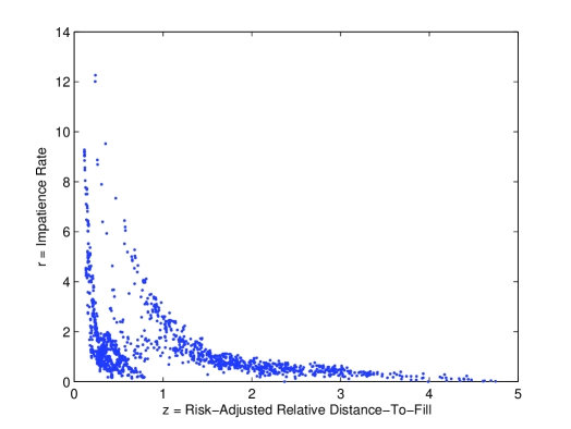
Figure 1: Impatience rate ($r$, y-axis) against risk-adjusted relative distance-to-fill ($z$, x-axis) for the sell side of the book. The fitting procedure reveals a power law for $r$, which is driven by both - the estimated volatility $s$ and the absolute distance-to-fill $D$. (FDAX, August 20, 2010)

The relationship demonstrated in Figure 1 provides evidence, that the impatience rate is primarily a function of the estimated volatility and the distance-to-fill $D$. A first conclusion is that in the GBM model the impatience rate is not constant across different levels. In particular it cannot extract solely the information content about the trade-off between a better fill price and a longer expected waiting time, but much rather it still contains information about the volatility and the distance-to-fill. Next, in Figure 2 we show a log-log plot which suppresses the power law relationship between $r$ and $z$ and reveals the different strains of this relationship for different levels of expected utility. The relative level of expected can be interpreted as indicative of prevailing market sentiment and therefore different levels of expected utility represent different market modes, and sharp changes in the absolute value of utility point to a sentiment shift.

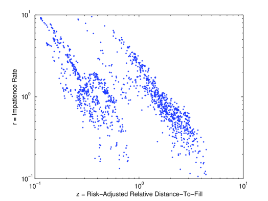
Figure 2: $\log_{10}$ of the impatience rate ($r$, y-axis) against $\log_{10}$ of the risk-adjusted relative distance-to-fill ($z$, x-axis) for the sell side of the book. Notice the different linear (exponential on a linear scale) strains, which indicate the same power relationship between $r$ and $z$ for different levels of the expected utility. (FDAX, August 20, 2010)

In figure 3 we present the expected utility compared to the mid-price through time. Changes in the direction of the expected utility, indicate numerical instability and can be interpreted as an indication, that a shift in sentiment of the respective market participants (here - the sellers), is taking place. A more detailed analysis showed that while indeed price direction and expected utility changes are concurrent, the latter is not a reliable predictor of the former.

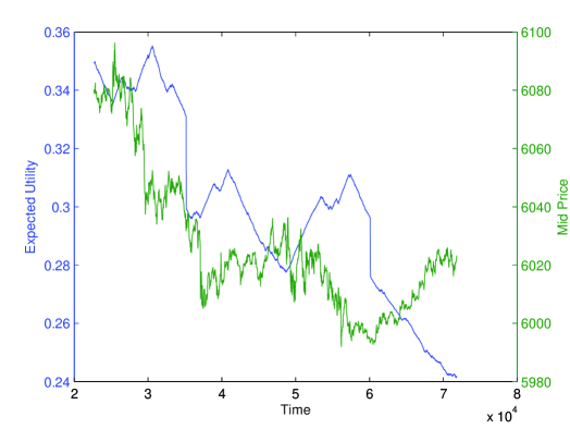
Figure 3: The expected seller utility $U$ (left axis) and the mid-price (right axis) through time (x-axis) on a single trading day. Notice the initial drop from the initial estimate to a level which is reflecting the actual expected utility given the impatience rate $r$, and the subsequent smoothness of the evolution of the utility. Jumps indicate a change in the utility level and correspond to a different linear strain in the relationship between $r$ and $z$, as demonstrated in the previous figure. (FDAX, August 20, 2010)

In Figure 4 a comparison of the impatience rate and the mid-price is given. One of the objectives of this research is to conclude whether the impatience rate is somehow indicative of future price movement, or if it contains any other piece of useful information. The intuition is that on, per example, the sell side of the book, an increasing impatience rate $r$ indicates, that sellers are becoming eager to get out of their holdings, so a price deterioration can be anticipated.

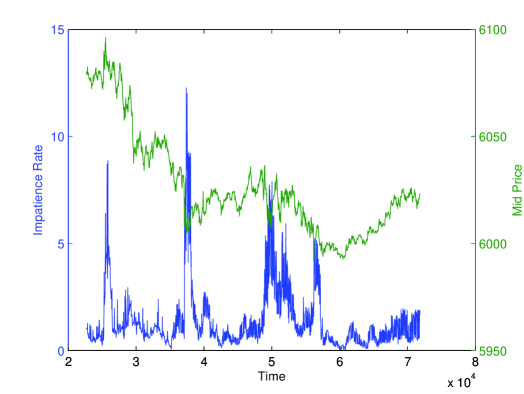
Figure 4: The seller impatience rate $r$ (left axis) and the mid-price (right axis) through time (x-axis) on a single trading day. Intuitively a rise in the seller impatience rate should precede or accompany a fall in the price. (FDAX, August 20, 2010)

While testing has revealed, that sharp changes in the mid-price are accompanied a shift in the opposite direction of the sell-side impatience rate, the direction of $r$ is not a reliable indicator of future price movements, since there are false outbreaks. Also price changes, which have not occurred abruptly enough, may not be captured by a significant change in $r$ and thus missed. Notice also how the impatience tends to fluctuate, around a stable state, when the price is trending sideways. This is a particular consequence of the fact that the impatience rate is a function of the distance-to-fill - the fluctuations indicate that the impatience rate needs to assume a different value for new values of $D$, in order to keep the expected seller utility smooth. As a result regression analysis has showed no significant relationship between the estimated impatience rate and future mid-price returns. The results for the buy-side of the LOB are similar and a side-by-side comparison of sell and buy side results can be seen in the appendix.

5 Volatility Smile

The results reveal that the impatience rate is not constant across LOB levels and in this model framework cannot be used as a consistent quantifier of the trade-off between a better fill price a longer expected time-to-execution. Further analysis suggested that the impatience rate in a GBM model is a function of the distance-to-fill and of the estimated volatility. Intuitively the market participants, who place their orders further out in the LOB, imply a much higher volatility than the observed. It seems as if traders who place orders at higher levels in the LOB are betting on a sharp price change in the desired direction. In order to analyse this further, we take a look at the LOB implied volatility, which we define to be the volatility $\sigma$ for which

$$U_{D}(r)=U_{D}(r,\sigma)=c$$ (14)

for some positive constant $c$. As we have already established, the impatience rate depends on $D$, and on $\sigma$, so we would like to separate and measure the two effects. To this end we choose an arbitrary, but reasonable, constant $c$ for the utility level and also fix the impatience $r$ at some constant level. Both are held constant throughout a whole trading day, and we fit for $\sigma$, to derive the implied volatility which keeps the impatience rate constant at $r$ and the expected utility level $U_{D}(r,\sigma)$ constant at a level $c$ for the entire trading day. What we discover is a volatility smile, being implied by the LOB, as is demonstrated in Figure 5. Essential this shows, that the GBM underweights limit orders at higher levels - the process’ volatility is insufficient for it to reach these limits in due time, so the volatility has to be tuned up to account for the dynamic equilibrium, and for market efficiency to hold.

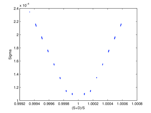
Figure 5: The volatility smile, as implied by the LOB. A scatter plot of the implied volatility $\sigma$ (y-axis) and the relative distance-to-fill $(S+D)/S$ (x-axis) form what resembles a volatility smile as known from equity options pricing. The plot reveals a whole day’s worth of data. $\sigma$ values to the left of one are derived from the bid-side of the LOB, and to the right - from the ask-side. This instance of the smile was derived for $U=0.2355$ and $r=0.5$ (FDAX, August 20, 2010)

The empirical work conclusively shows, that in a GBM setting, there is no unifying impatience rate across the different levels in the LOB. It has turned out that it is a function of both - the volatility term $\sigma$ of the stochastic process, and of $|D|$ - the distance-to-fill. It is inversely related to the volatility, i.e. the higher the volatility, the lower the impatience rate, on either side of the book. It means that it becomes “easier” for the process to reach an order, which is at a higher level in the book, which is in turn necessary due the assumption that the expected utility is the same at all levels of the book, and evolves smoothly through time.

In the same way, the impatience rate is a function of the distance-to-fill. It plays the role of a “volatility-compensator”, keeping the expected utility $U$ constant across levels for different values of $|D|$ . The impatience rate needs to be very small for large $|D|$ in order to compensate for the decrease in utility, as $\tau$ becomes too big. Since the volatility is fixed by empirical observations, and $\mathbb{E}[\tau]$ is known to grow exponentially with rising distance, it is a direct consequence of the GBM framework, that $r$ follows an exponential decay law for an increasing $|D|$ and a falling $\sigma$.

The inverse power-law between the impatience rate and the observed volatility is especially clearly observable in the volatility smile. This surprising discovery highlights the fact that in order to achieve utility equilibrium one has to tune up the process’ volatility, so that limit orders placed further away from the mid-price have a higher chance of execution. Intuitively one may argue, that market participants place limit orders further out in the LOB, because they anticipate a large block of orders being placed at once, so that lower level limit orders get immediately filled, leaving the agent’s order as the best or even filling it.

A critical argument for jump augmentation is based on the observed “volatility smile”, a phenomenon well known from option pricing. There are already many models in options theory which account for the smile. Regarding the principle idea of the solution, there are two broad classes of approaches to incorporate this phenomenon in the price process. One is to assume a stochastic process for the volatility term in front of the Brownian motion. The other is to add a jump process to the Brownian motion. While it might seem somewhat natural that the volatility itself should also be a process rather than a constant term, the dynamics that are usually used to model the evolution of the volatility through time are not necessarily intuitive. On the other hand, the idea, that price processes have jumps is considered characteristic of financial time series and is readily observable. In combination with the intuition, that limit order traders position themselves at the outer levels in anticipation of a block-trade, or a sharp price movement, we are lead to extend the GBM to a jump-diffusion by incorporating a jump process, i.e. a process of the form:

$$\text{d}S_{t}=\mu S_{t}\text{d}t+\sigma S_{t}\text{d}B_{t}+S_{t}\text{d}J_{t},\quad J_{t}=\sum_{i=i}^{N_{t}}Y_{i}$$

where $J_{t}$ is a time-homogeneous compound Poisson process, whose jump sizes $(Y_{i})_{i\in\mathbb{N}}$ are a family of independently and identically distributed (iid) random variables.

6 A Jump-Diffusion Setting

Lead by the observation of a volatility smile and the intuition that far-off limit orders are underweighted, in the sense that in the geometric Brownian motion (GBM) framework high-level orders are too difficult to hit, we extend our asset price model to include jumps. In this way we will be able to account for the observed empirical phenomena and serve intuition. Due to the increased flexibility of the models we are also certain to obtain a better fit of a period-wise constant impatience rate to the market data.

Since the success of the Black-Scholes-Merton formula for equity option valuation, which underlies a geometric Brownian motion, a number of jump-diffusion models have been proposed as an extension to the original model. We are going to use the Double Exponential Jump Diffusion (DEJD) model, as proposed by Kou in [Kou02] and extensively studied by Kou and Wang in [KW03]. Our choice is lead by our specific interest of the Laplace transform of the first passage time of the asset price. As is demonstrated in [KW03], the model offers a closed-form solution (up to finding the zeros of a rational function) for the Laplace transform.

The DEJD model of the asset mid-price $(S_{t})_{t\geq 0}$ is specified by the stochastic differential equation

$$\text{d}S_{t}=S_{t}\mu\text{d}t+S_{t}\sigma\text{d}B_{t}+S_{t}\text{d}\left(\sum_{i=1}^{N_{t}}(V_{i}-1)\right)$$ (15)

where $N_{t}\sim\textsf{Poi(}\lambda t\textsf{)}$ is a Poisson process with intensity $\lambda$, and

$$Y:=\log(V_{1})\sim\textsf{dexp}(p,q,\eta_{1},\eta_{2}\textsf{)}$$ (16)

iid random variables, distributed according to the asymmetric double-exponential law with the density

$$f_{Y}(t)=p\eta_{1}\exp(-\eta_{1}t)\textbf{1}_{\{t\geq 0\}}+q\eta_{2}\exp(-\eta_{2}t)\textbf{1}_{\{t<0\}}$$ (17)

$$\eta_{1}>2,\;\eta_{2}>2,$$

$$p,\;q>0,\quad p+q=1$$

The model parameters can be understood as follows: at any time $p$ is the probability of an upward jump, and $q=1-p$ is the probability of a downward jump. The mean jump-sizes are $1/\eta_{1}$ and $1/\eta_{2}$ for an up-jump and a down-jump respectively. At each point in time only one jump can occur, and the occurrence of jumps is modelled by a homogeneous Poisson process with a constant intensity rate of $\lambda$, meaning that the mean number of jumps up to time $t$ is $\lambda t$. All driving process of the model price, $N(t)$, $B_{t}$ and $(V_{i})_{i\in\mathbb{N}}$ are assumed to be independent, although in [Kou02] it is suggested that this assumption can be relaxed. For the purposes of this paper this possibility will not be further investigated.

Theorem 6.1.

The solution of the SDE (15) is given by the process

$$S_{t}=S\exp\left(\left(\mu-\dfrac{\sigma^{2}}{2}\right)t+\sigma B_{t}\right)\prod_{i=1}^{N(t)}V_{i}$$ (18)

Proof.

See the appendix. ∎

For convenience we adopt the following representation of $Y$:

$$Y\stackrel{{\scriptstyle\mathcal{D}}}{{=}}U\xi^{+}-(1-U)\xi^{-}$$ (19)

where $U\sim\textsf{Ber(}p\textsf{)}$ is a Bernoulli random variable, indicating that an up-jump occurs with probability $p$, $\xi^{+}$ and $\xi^{-}$ are both exponential random variables with means $1/\eta_{1}$ and $1/\eta_{2}$ respectively, corresponding to the mean up-jump and mean down-jump sizes. All three random variables are assumed to be independent.

Theorem 6.2.

The asset mid-price model specified by (18) and (19) where $Y=\log(V_{1})$ has the following properties

• $\mathbb{E}Y=\frac{p}{\eta_{1}}-\frac{q}{\eta_{2}}$ and $\mathbb{V}Y=pq\left(\frac{1}{\eta_{1}}+\frac{1}{\eta_{2}}\right)^{2}+\left(\frac{p}{\eta_{1}^{2}}+\frac{q}{\eta_{2}^{2}}\right)$;

• $\mathbb{E}[V]=q\frac{\eta_{2}}{\eta_{2}+1}+p\frac{\eta_{1}}{\eta_{1}-1},$ and
  $\mathbb{V}[V]=p\dfrac{\eta_{1}}{\eta_{1}-2}+q\dfrac{\eta_{2}}{\eta_{2}+2}-\left(p\dfrac{\eta_{1}}{\eta_{1}-1}+q\dfrac{\eta_{2}}{\eta_{2}+1}\right)^{2}$, $\eta_{1},\eta_{2}>2$;

• The first two moments of the “Poisson product” $P_{t}:=\prod_{i=1}^{N_{t}}V_{i}$ are:

  • $\mathbb{E}[P_{t}]=\exp(t\lambda(\mathbb{E}[V]-1))$ and

  • $\mathbb{E}[P_{t}^{2}]=\exp(t\lambda(\mathbb{E}[V^{2}]-1))$;

• $\mathbb{E}S_{t}=S\exp(\mu t)\mathbb{E}[P_{t}]$ and $\mathbb{V}S_{t}=S^{2}e^{2\mu t}\left(e^{\sigma^{2}t}\mathbb{E}[P_{t}^{2}]-\mathbb{E}[P_{t}]^{2}\right)$

• For $l(\Delta t)$, the log-returns over a period $\Delta t$, we have:

  • $\mathbb{E}[l(\Delta t)]=\left(\mu-\frac{\sigma^{2}}{2}\right)\Delta t+\lambda\left(\frac{p}{\eta_{1}}-\frac{q}{\eta_{2}}\right)\Delta t\quad$ and

  • $\mathbb{V}[l(\Delta t)]=\sigma^{2}\Delta t+\lambda\Delta t\left(\frac{2p}{\eta_{1}^{2}}+\frac{2q}{\eta_{2}^{2}}\right)$.

Proof.

See the appendix. ∎

Observing that $\mathbb{V}[V]=\infty$ for $\eta_{1}\leq 2$, as shown in the proof of b), we are lead to impose this constraint when modelling the asset price. Since there is no intuitive reason to prefer a priori any price direction we make the same assumption for $\eta_{2}$ in (17). It essentially means, that mean jump sizes cannot exceed 50%.

6.1 First Passage Time Results

Here we present the results of Kou/Wang for the first passages times of a double exponential jump diffusion process, as given in [KW03]. Consider the DEJD proces

$$X_{t}=\sigma B_{t}+\mu t+\sum_{i=1}^{N_{t}}Y_{i};\quad X_{0}:=0$$ (20)

where $(B_{t})_{t\geq 0}$ is a standard Brownian motion, $(N_{t})_{t\geq 0}$ is a Poisson process with intensity rate $\lambda$, $\mu$ and $\sigma>0$ are respectively the constant drift and the volatility of the diffusion part of the process. The family of the jump-sizes $(Y_{i})_{i\in\mathbb{N}}$ is independent and identically distributed according to a a double-exponential distribution with density $f_{Y}$ as given in (17). We are interested in the Laplace transform of $\tau_{b}$, the random variable specified by the first passage time of a boundary $b$:

$$\tau_{b}:=\inf_{t\geq 0}\{X_{t}\geq b\},\quad b>0$$ (21)

The infinitesimal generator of the jump diffusion process (20) is given by

$$\mathcal{L}u(x)=\dfrac{1}{2}\sigma^{2}u^{\prime\prime}(x)+\mu u^{\prime}(x)+\lambda\int_{-\infty}^{\infty}\big{(}u(x+y)-u(x)\big{)}f_{Y}(y)\text{d}y$$ (22)

for all twice continuously differentiable functions $u(x)$. Further, suppose $\theta\in]-\eta_{2},\eta_{1}[$. The moment generating function of the jump size $Y$ is given by:

$$\mathbb{E}[\exp(\theta Y)]=\dfrac{p\eta_{1}}{\eta_{1}-\theta}+\dfrac{q\eta_{2}}{\eta_{2}+\theta},$$ (23)

from which the moment generating function of $X_{t}$ can be obtained as

$$\varphi(\theta,t):=\mathbb{E}[\exp(\theta X_{t})]=\exp(G(\theta)t),$$

where the function $G(\cdot)$ is defined as

$$G(x):=x\mu+\dfrac{1}{2}x^{2}\sigma^{2}+\lambda\left(\dfrac{p\eta_{1}}{\eta_{1}-x}+\dfrac{q\eta_{2}}{\eta_{2}+x}-1\right)$$ (24)

Lemma 6.1.

The equation

$$G(x)=\alpha\;\text{ for all }\;\alpha>0$$ (25)

has exactly four roots: $\beta_{1,\alpha}$, $\beta_{2,\alpha}$, $-\beta_{3,\alpha}$, $-\beta_{4,\alpha}$ where

$$0<\beta_{1,\alpha}<\eta_{1}<\beta_{2,\alpha}<\infty,\quad 0<\beta_{3,\alpha}<\eta_{2}<\beta_{4,\alpha}<\infty$$

Proof.

Cf. [KW03] (page 507, Lemma 2.1). ∎

Theorem 6.3.

For any $\alpha\in]0,+\infty[$, leta $\beta_{1,\alpha}$ and $\beta_{2,\alpha}$ be the only positive roots of the equation

$$\alpha=G(x),$$

where $0<\beta_{1,\alpha}<\eta_{1}<\beta_{2,\alpha}<+\infty$. Then the Laplace transform of $\tau_{b}$ is given by:

$$\mathbb{E}\left[e^{-\alpha\tau_{b}}\right]=\dfrac{\eta_{1}-\beta_{1,\alpha}}{\eta_{1}}\dfrac{\beta_{2,\alpha}}{\beta_{2,\alpha}-\beta_{1,\alpha}}e^{-b\beta_{1,\alpha}}+\dfrac{\beta_{2,\alpha}-\eta_{1}}{\eta_{1}}\dfrac{\beta_{1,\alpha}}{\beta_{2,\alpha}-\beta_{1,\alpha}}e^{-b\beta_{2,\alpha}}$$ (26)

Proof.

Cf. [KW03] (page 509, Theorem 3.1). ∎

Again, a simple transform is needed in order to apply the result from the previous theorem to our process given by (18). For $D>0$ consider:

$$\tau_{S+D}^{\text{exp}} =\inf_{t\geq 0}\{S_{t}\geq S+D\}$$

$$=\inf_{t\geq 0}\left\{S\exp\left(\left(\mu-\dfrac{\sigma^{2}}{2}\right)t+\sigma B_{t}+\sum_{i=1}^{N_{t}}Y_{i}\right)\geq S+D\right\}$$

$$=\inf_{t\geq 0}\Big{\{}\underbrace{\left(\mu-\dfrac{\sigma^{2}}{2}\right)}_{\hat{\mu}}t+\sigma B_{t}+\sum_{i=1}^{N_{t}}Y_{i}\geq\underbrace{\log\left(\dfrac{S+D}{S}\right)}_{z}\Big{\}}$$

$$=\hat{\tau}_{z}$$ (27)

So the expected utility for the ask side of the LOB (i.e. for the sellers) is given by substituting $z$ for $b$ in (26), and calculating $\beta_{1,r}$ and $\beta_{2,r}$ by solving (25) with $\hat{\mu}$ and $z$:

$$G(\beta_{i})=r,\quad i\in\{1,2\}$$

$$\beta_{i}\hat{\mu}+\dfrac{1}{2}\beta_{i}^{2}\sigma^{2}+\lambda\left(\dfrac{p\eta_{1}}{\eta_{1}-\beta_{i}}+\dfrac{q\eta_{2}}{\eta_{2}+\beta_{i}}-1\right)=r$$

where the two roots $$\beta_{1} \beta_{2}$$ and are in the following intervals:

$$0<\beta_{1,\alpha}<\eta_{1}<\beta_{2,\alpha}<\infty$$

Observe, that while in the GBM setting, we had direct access to a formula for the first hitting time regardless of whether the boundary was above, or below the starting point of the process, Theorem 6.3 only provides a formula for higher boundaries. So we need to make a distinct transform for the bid (i.e. buy) side of the LOB. Now, consider for $D>0$ the following:

$$\tau_{S-D} =\inf_{t\geq 0}\{S_{t}\leq S-D\}$$

$$=\inf_{t\geq 0}\Bigg{\{}\underbrace{-\left(\mu-\dfrac{\sigma^{2}}{2}\right)}_{\hat{\mu}}t-\sigma B_{t}-\sum_{i=1}^{N_{t}}Y_{i}\geq\underbrace{-\log\left(\dfrac{S-D}{S}\right)}_{z}\Bigg{\}}$$

$$\stackrel{{\scriptstyle\mathcal{D}}}{{=}}\inf_{t\geq 0}\left\{\hat{\mu}t+\sigma B_{t}-\sum_{i=1}^{N_{t}}Y_{i}\geq z\right\}$$

$$\stackrel{{\scriptstyle\mathcal{D}}}{{=}}\inf_{t\geq 0}\left\{\hat{\mu}t+\sigma B_{t}+\sum_{i=1}^{N_{t}}\hat{Y_{i}}\geq z\right\}$$

$$=\hat{\tau}_{z}$$ (28)

where the first transform in probability is due to the reflection principle, and the second due to

$$Y=U\xi^{+}-(1-U)\xi^{-}\Rightarrow-Y=-(1-U)\xi^{-}-U\xi^{+}$$ (29)

where $$Y\sim\textsf{dexp(}p,q,\eta_{1},\eta_{2} \hat{Y}\sim\textsf{dexp(}q,p,\eta_{2},\eta_{1}$$), so that for )

$$\hat{Y}\stackrel{{\scriptstyle\mathcal{D}}}{{=}}-Y.$$ (30)

Obviously in the DEJD model there are significantly more parameters to be either estimated, or fitted. While in the GBM setting we could extract the impatience rate and expected utility by estimating the drift and volatility of log-returns, and imposing constraints such as keeping $r$ and $U_{D}(r)$ constant, a similar strategy would have only limited success in the DEJD framework. A fundamental trade-off between keeping the model as flexible as possible and imposing new constraints is at hand, because the former carries a significant risk of overfitting, and the latter might not converge for a large class of pre-set parameters. Next we show how to separate the diffusive volatility from the jump-part contribution to total process volatility, which reduces the number of parameters needed to fit.

6.2 Parameter Calibration to Market Data

The main difference in this process, compared to a diffusion, is that a point estimate of $\mathbb{V}[l(\Delta)t]$ from observed data is an estimate for the sum of the diffusive and the jump-part variances, as is shown in Theorem 6.1. We will therefore make use of the bipower variation introduced by Brandorff-Nielsen and Shephard in [BNS04]. Consider the realized variance over a period $N\Delta t$:

$$RV_{N\Delta t}\left(\frac{1}{N}\right):=\sum_{j=1}^{N}R_{j,\Delta t}^{2}(N)$$

where $N$ is the sampling frequency and $R_{j,\Delta t}^{2}(N)$ is the log return in the time span from $(j-1)\Delta t$ to $j\Delta t$. Notice that $RV_{N\Delta t}$ is an estimate of the total process variance over the whole sampling period $N\Delta$. It can be shown, that

$$\text{for }\;m\to\infty\;RV_{m\cdot\frac{\Delta tN}{m}}\left(\frac{1}{m}\right)\to\mathbb{V}[l(N\Delta t)],$$

i.e. by increasing the sampling frequency over the same interval $N\Delta t$, the realized variance converges to the the process’ total variance over the period $N\Delta t$. Consider further the bipower variation:

$$BV_{N\Delta t}\left(\frac{1}{N}\right)=\dfrac{\pi}{(1-2/N)2}\sum_{j=3}^{N}\left|R_{j,\Delta t}^{2}(N)\right|\left|R_{j-2,\Delta t}^{2}(N)\right|,$$

which is shown to converge for an increasing sampling frequency to the diffusive part of the total variance of the process over the whole sampling period $N\Delta t$, i.e.

$$\text{for }\;m\to\infty\;BV_{m\cdot\frac{\Delta tN}{m}}\left(\frac{1}{m}\right)\to\sigma^{2}N\Delta t$$

So from the log-returns $l(\Delta t)$ we can estimate the diffusive $\sigma^{2}$ by:

$$\sigma^{2}\Delta t=\dfrac{BV_{N\Delta t}\left(\frac{1}{N}\right)}{N}$$ (31)

and for the jump part we can use:

$$\mathbb{V}[l(\Delta t)]-\sigma^{2}\Delta t=\dfrac{RV_{N\Delta t}\left(\frac{1}{N}\right)-BV_{N\Delta t}\left(\frac{1}{N}\right)}{N},$$

which in combination with the estimate for $$\sigma^{2}$$ and with Theorem 6.1 e) leads to

$$\lambda\Delta t\left(\frac{2p}{\eta_{1}^{2}}+\dfrac{2q}{\eta_{2}^{2}}\right)=\dfrac{RV_{N\Delta t}\left(\frac{1}{N}\right)-BV_{N\Delta t}\left(\frac{1}{N}\right)}{N},$$ (32)

quantifying the jump-part contribution to the process’ total variance. Due to sampling errors however, this expression may take a negative value, so in order to avoid this in our empirical work we cap the bipower variation by the realized variance:

$$\widehat{BV}_{N\Delta t\left(\frac{1}{N}\right)}:=\min\left\{BV_{N\Delta t}\left(\frac{1}{N}\right),RV_{N\Delta t}\left(\frac{1}{N}\right)\right\}$$ (33)

Again, as in the GBM setting, we choose $N=30$ and base our rolling estimates at $t$ on observed log-returns from $t-N-1$ to $t-1$. Still, including the diffusive drift $\mu$, we have a total of five parameters (as $q=1-p$) to estimate from a single constraint. For this reason we assume, that the process has no drift, arguing that price level changes come about jump-wise, and that price movement between jumps is driven only by Brownian motion scaled by its diffusive $\sigma$. We can also add another constraint from the observed rolling mean of the log-returns:

$$\overline{m}=-\dfrac{BV_{N\Delta t}\left(\frac{1}{N}\right)}{2N}+\lambda\Delta t\left(\frac{p}{\eta_{1}}-\dfrac{q}{\eta_{2}}\right)$$ (34)

Now there are four free parameters and two constraints. Additional assumptions and constraints may include either, or all of the following (superscripts indicate the time of the data point):

• $\eta_{1}^{j}=\eta_{2}^{j}$, or $\left(\eta_{1}^{j}-\eta_{2}^{j}\right)^{2}\leq\epsilon$, which amounts to assuming that mean jump-sizes are essentially the same for up-jumps and down-jumps. The only source of asymmetry in the model derives from the probability $p$ that an up-jump occurs, given that the price process jumps at all.

• $\left(\lambda^{j}-\lambda^{j-1}\right)^{2}\leq\epsilon$;

• $\left(p^{j}-p^{j-1}\right)^{2}\leq\epsilon$

• $\left(\eta_{i}^{j}-\eta_{i}^{j-1}\right)^{2}\leq\epsilon$ for $i=1,2$.

All of these constraints make sense, and especially the first one would be the most stringent and effective, as the estimation problem would then be to derive three parameters from two constraints. However, readily available optimization procedures would not converge when this constraint is introduced for reasons explained in the next paragraph.

Another feature of the fitting is that we now need to fit the impatience rate and expected utility for the bid and for the ask side simultaneously. While in the GBM setting the process parameters for the bid and the ask side were the same and did not need fitting, which allowed us to solve for the impatience rate and the expected utility on each side of the book consecutively, in the DEJD setting we must assume that sellers and buyers have the same view of the underlying process, so we need to fit two impatience parameters $r^{\text{ask}}$ and $r^{\text{bid}}$ in parallel, while still under the assumption that either of the expected utilities $U^{\text{bid}}$ and $U^{\text{ask}}$ is step-wise approximately constant and evolves smoothly. This of course makes the fitting procedure much more difficult and potentially unstable with off-the-shelf optimization techniques. In fact, this is the reason why with the introduction of more stringent constraints from the above list, the optimization fails to converge - we have found that for a target function similar to the one from GBM framework minimizing the error for one side of the book only, an optimization algorithm with all of the above constraints introduced would converge.

On one hand, fitting both sides simultaneously restrains available optimization techniques from introducing constraints. On the other hand fitting the stochastic process’ driving parameters on two separate and independent sets of data in parallel is of and in itself an additional constraint, which should discipline the optimization algorithm and provide insurance against parameter redundancy. Since we can optimize one side of the book imposing all of the constraints, we suppose a more careful analysis of the parameter domain for the optimization problem should lead to an algorithm which converges. This, however, is beyond the scope of this paper, as it is a numerically challenging problem, which departs from the research of price dynamics implications of the LOB. Furthermore, with only the last constraint from the list above, we achieve reasonable results.

Following is a pseudo-code representation of Algorithm 2 for the estimation of the impatience rate in a DEJD setting. The inputs are starting utilities and impatience rates for both sides of the book, and a vector of process starting parameters $P$, which cannot be directly estimated and need fitting, that is $\lambda$, $\eta_{1}$, $\eta_{2}$ and $p$. The outputs are two vectors of utilities, two vectors of impatience rates and a set of price process parameters derived by our fitting procedure.

Algorithm 2 Estimation of the impatience rate in a DEJD setting

Inputs: N, steps, $U_{0}^{\text{ask}}$, $r_{0}^{\text{ask}}$, $U_{0}^{\text{bid}}$, $r_{0}^{\text{bid}}$, $s^{2}$, $m$

1:  $r_{0}:=\big{(}r^{\text{ask}}_{0},r_{0}^{\text{bid}}\big{)}\in\mathbb{R}^{2}_{+}$

2:  $U_{0}:=\big{(}U^{\text{ask}}_{0},U_{0}^{\text{bid}}\big{)}\in\mathbb{R}^{2}_{+}$

3:  for i=1:N  do

4:     while $\text{error(r)}>\epsilon\;\&\;\text{Tolerance}>\delta$ do

5:        $r_{i}:=\min_{r>0.01}\{\text{error(r)}\}$

6:        s.t. constraints (31),(32),(33), (34) & $\left(\eta_{i}^{j}-\eta_{i}^{j-1}\right)^{2}\leq\epsilon$ for $i=1,2$

7:        WHERE error(r) is

8:        calculate $U_{j}^{\text{ask}}$ according to (2), (27), using $P$, $r^{\text{ask}}$

9:        calculate $U_{j}^{\text{bid}}$ according to (2), (28), using $P$, $r^{\text{bid}}$

10:        error(r) = $\left(\dfrac{(U^{\text{ask}}_{j}-U^{\text{ask}}_{j-1})}{0.5(U^{\text{ask}}_{j}+U^{\text{ask}}_{j-1})}\right)^{2}+\left(\dfrac{(U^{\text{bid}}_{j}-U^{\text{bid}}_{j-1})}{0.5(U^{\text{bid}}_{j}+U^{\text{bid}}_{j-1})}\right)^{2}$

11:        error(r) = $\left(\dfrac{(r^{\text{ask}}_{j}-r^{\text{ask}}_{j-1})}{0.5(r^{\text{ask}}_{j}+r^{\text{ask}}_{j-1})}\right)^{2}+\left(\dfrac{(r^{\text{bid}}_{j}-r^{\text{bid}}_{j-1})}{0.5(r^{\text{bid}}_{j}+r^{\text{bid}}_{j-1})}\right)^{2}$

12:        error(r) =error(r)/4

13:     end while

14:  end for

Outputs: $U=\big{(}U^{\text{ask}},U^{\text{bid}}\big{)}\in\mathbb{R}^{2\times N}_{+}$, $r=\big{(}r^{\text{ask}},r^{\text{bid}}\big{)}\in\mathbb{R}^{2\times N}_{+}$, $P\in\mathbb{R}^{4\times N}$

As already noted, this problem is numerically challenging. Very sensible tuning of optimization parameters concerning convergence tolerance is needed. The problem is further complicated, by the fact that the function $G$ (cf. Theorem 6.3) is so poorly conditioned, that finding its roots in the specified intervals (where the function is differentiable) becomes very hard. For this reason we must use an efficient implementation of the very robust but time-consuming bisection algorithm. Note that in order to apply bisection the function $G$ needs to be monotonic and continuous over the specified interval, and its values at the interval boundaries to have different signs. This is verified in Lemma 6.1.

7 Results For a Jump-Diffusion

The double-exponential jump-diffusion (DEJD) proves to be much better suited to model an equilibrium in the LOB under the assumption of a constant impatience rate across levels, given an established market regime (see Figure 8). The induced fat-tailed distribution of log-returns makes orders further out in the book more accessible, than in a GBM setting. We further establish, that in order to achieve an equilibrium of the LOB, as reflected by the consistency of the impatience rate, the underlying process cannot be e GBM.

We illustrate our findings by showing a representative day, again August 20, 2010, and again only showing results for the sell-side of the LOB. Figure 6 shows the expected utility in the DEJD setting. While still essentially flat for established market regimes, its choppiness is indicative of partial numerical instability, a problem outlined in the previous section. Nonetheless, the success of the DEJD over the GBM is clearly demonstrated in Figure 7, where the evolution of the impatience rate is shown. It is very stable for established market modes and changes spike-wise to indicate that a new market regime has been established. Regression analysis has however showed, that as in the GBM case, the impatience rate is not indicative of future price movements. It serves very much as an anchor which allows for consistent comparison of limit orders at different levels in the LOB, as long as market sentiment remains unchanged.

Figure 8 clearly shows, that in a DEJD setting, an approximately constant impatience rate can be derived. It shows the impatience rate as a function of the distance-to-fill in the course of a whole day. Highlighted are the values for two periods when market regime was unchanged, and the expected utility was constant in each period. Since the implied impatience rates form a flat line across all distances for a given level of utility, they are not dependent on the limit order level. This means that $r$ can be used as reliable and well-defined quantifier of the trade-off between waiting longer for a better price against waiting less for a worse price.

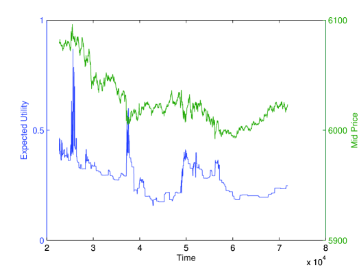
Figure 6: Expected utility (left axis) and mid-price (right axis) for the sell side of the book in the DEJD setting. The utility is not as smooth as in the GBM setting, but still a very good fit. (FDAX, August 20, 2010)

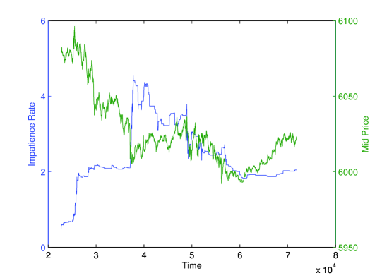
Figure 7: Impatience rate (left axis) and mid-price (right axis). The DEJD framework provides for a smooth, level-independent $r$, where the GBM setting fails. (FDAX, August 20, 2010)

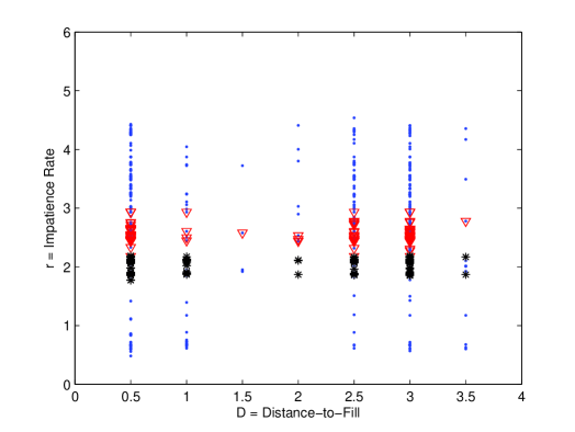
Figure 8: $r$ against $D$. Apparently much less noisy than the GBM framework, but at first sight still very scattered. Notice, however the black stars ($r$ from $t=$3 to $t=$3.75) and the red triangles ($r$ from $t=$5.25 to $t=$5.75), as a function of $D$ in two different market modes. In the absence of market sentiment shifts $r$ is nearly constant. Changes in $r$ could indicate shift in sentiment. It is also apparent that in contrast to the GBM setting, the in the DEJD model impatience rate is a function of neither the distance-to-fill, nor the volatility.

8 Conclusion

We have shown that the assumption of an equilibrium in the limit order book (LOB) is not consistent with the price dynamics given by a geometric Brownian motion (GBM). Instead, in equilibrium, the LOB implies a volatility smile that is reminiscent of, but unrelated to, the one known from option-pricing. This observation necessarily leads to a fat-tailed distribution of log-returns. The most natural explanation of this phenomenon is the occurrence of jump processes in the price dynamics.

We further demonstrate how an impatience rate is implied from empirical observations, so that it is consistent with the assumption of market efficiency.

There are several directions for further research of the proposed framework. A natural extension would be the study of different jump-diffusion models, which provide greater parameter stability. In addition one could investigate stochastic volatility models as an alternative to incorporating the volatility smile. Furthermore it would be instructive to compare the jump parameters presented in this paper with the results from standard techniques that are based on a direct analysis of the time-series.

9 Acknowledgement

We would like to thank Gregor Svindland for constructive comments on this paper.

Appendix A Additional Plots

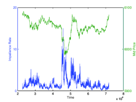
(a) GBM Buyer

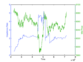
(b) DEJD Buyer

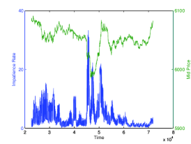
(c) GBM Seller

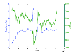
(d) DEJD Seller

Figure 9: Impatience rates and mid-price.

(a) GBM Buyer

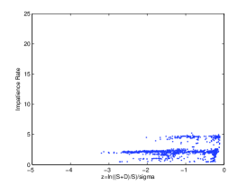
(b) DEJD Buyer

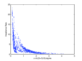
(c) GBM Seller

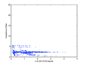
(d) DEJD Seller

Figure 10: Impatience rates against the risk-adjusted realtive distance-to-fill $z=\frac{\log(S+D)/S}{\sigma}$.

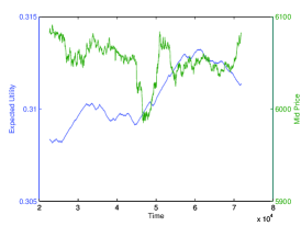
(a) GBM Buyer

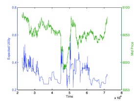
(b) DEJD Buyer

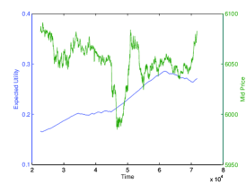
(c) GBM Seller

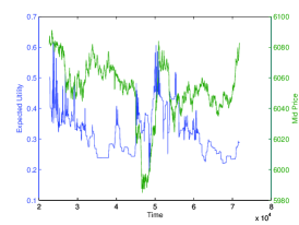
(d) DEJD Seller

Figure 11: Expected utilities and mid-price.

Appendix B Proof of Theorem 6.1

A number of preliminary results are due, in order to prove the statement. We begin by formulating the It$\hat{\text{o}}$ lemma for semi-martingales, (eg. jump-diffusions), and then apply it to our process to obtain the solution.

Lemma B.1 (It$\hat{\text{o}}$’s Lemma for Semi-Martingales).

Let $X$ be a semi martingale, and let $f$ be real $C^{2,1}$ function. Then $f(X,t)$ is again a semi-martingale, and the following formula holds:

$$df(X_{t},t-) =f_{t}(X_{t},t-)\text{d}t+f_{x}(X_{t-},t-)\text{d}X_{t}+\dfrac{1}{2}f_{xx}(X_{t-},t-)\text{d}\langle X\rangle^{c}_{t}$$

$$+\Delta f(X_{t},t-)-f_{x}(X_{t-},t-)\Delta X_{t}$$ (35)

with the following notations:

$$f_{x}(X,t) :=\dfrac{\partial f}{\partial X}(X,t),\quad f_{t}(X,t):=\dfrac{\partial f}{\partial t}(X,t),\quad f_{xx}(X,t):=\dfrac{\partial^{2}f}{\partial X^{2}}(X,t),$$

$$t- :=\lim_{\epsilon\downarrow 0}t-\epsilon,\quad\Delta X_{t}:=X_{t}-X_{t-},$$

$$\quad\Delta f(X_{t},t-) :=f(X_{t},t-)-f(X_{t-},t-).$$

Also $\text{d}\langle X\rangle_{t}^{c}$ is the differential of the quadratic variation process of the continuous part of $X_{t}$.

Proof.

A proof is given in [Pro90], p. 78. ∎

As a consequence the following corollary for the Dol$\acute{\text{e}}$ans-Dade stochastic exponential for semi-martingales can be formulated:

Corollary B.1 (Stochastic Exponential for Semi-martingales).

Let $X_{t}$ be a semi-martingale, $X_{0}=0$. Then there exists a unique semi-martingale $Z_{t}$ satisfying $\text{d}Z_{t}=Z_{t-}\text{d}X_{t}$ with $Z_{0}=1$. $Z_{t}$ is given by:

$$Z_{t}=\exp\left(X_{t}-\dfrac{1}{2}\langle X\rangle_{t}^{c}\right)\prod_{s\leq t}\Big{(}(1+\Delta X_{s})\exp(-\Delta X_{s})\Big{)}$$ (36)

Proof.

Cf. [Pro90], p.84. ∎

Proof of Theorem 6.1 .

Consider the following function

$$f(x,t):=xe^{\mu t},\;f_{x}(x,t)=e^{\mu t},\;f_{xx}(x,t)=0,\;f_{t}(x,t)=\mu xe^{\mu t}=\mu f(x,t).$$

We look for a solution of the form;

$$X_{t}=C_{t}e^{\mu t}$$

for some semi-martingale $C_{t}$. Applying the It$\hat{\text{o}}$-formula for semi-martingales we obtain:

$$\text{d}X_{t}=df(C_{t},t)=e^{\mu t}\text{d}C_{t}+\mu C_{t}e^{\mu t}\text{d}t$$

Notice that under the assumption $X_{t}=C_{t}e^{\mu t}$ the SDE can be rewritten as:

$$\text{d}X_{t}=C_{t}e^{\mu t}(\sigma\text{d}B_{t}+\text{d}J_{t}+\mu\text{d}t)$$

Comparing the last two equations, we conclude that:

$$\text{d}C_{t}=C_{t}(\sigma\text{d}B_{t}+\text{d}J_{t}),$$

and by virtue of the previous corollary, we know that the unique solution for $C_{t}$ is given by:

$$C_{t} =S\exp\left(\sigma B_{t}+\sum_{i=1}^{N_{t}}(V_{i}-1)-\dfrac{1}{2}\sigma^{2}t\right)\prod_{i=1}^{N_{t}}V_{i}\exp\big{(}-(V_{i}-1)\big{)}$$

$$=S\exp\left(\sigma B_{t}-\dfrac{1}{2}\sigma^{2}t\right)\prod_{i=1}^{N_{t}}V_{i},$$

which yields

$$X_{t} =C_{t}e^{\mu t}=\exp\left(\left(\mu-\dfrac{\sigma^{2}}{2}\right)t+\sigma B_{t}\right)\prod_{i=1}^{N_{t}}V_{i},$$

concluding the proof. ∎

Note that (18) is the same as:

$$S_{t}=S\exp\left(\left(\mu-\dfrac{\sigma^{2}}{2}\right)t+\sigma B_{t}+\sum_{i=1}^{N(t)}Y_{i}\right)$$ (37)

Appendix C Proof of Theorem 6.2

Definition C.1 (Poisson Process).

A right-continuous process $(N_{t})_{t\geq 0}$ with state space $\mathbb{N}_{0}$ is a time homogeneous Poisson process with intensity rate $\lambda$ iff the following is true:

• $N_{0}=0$ a.s.;

• the process has stationary, independent increments, which are Poisson distributed, i.e. for all $s,t\geq 0$ $N_{s+t}-N_{s}\sim\text{Poi(}\lambda t\text{)}$.

Definition C.2 (Compound Poisson Process).

Let $(N_{t})_{t\geq 0}$ be a time homogeneous Poisson process with intensity rate $\lambda$ and $(Y_{n})_{n\in\mathbb{N}}$ a family of iid random variables, and let the family further be independent of $(N_{t})_{t\geq 0}$. The process $(C_{t})_{t\geq 0}$, defined by

$$C_{t}:=\sum_{i=1}^{N_{t}}Y_{i},\quad t\geq 0$$

is called a compound Poisson process.

Lemma C.1.

For a time homogeneous compound Poisson process $(C_{t})_{t\geq 0}$ with intensity rate $\lambda$ and square-integrable $Y_{1}$ the following holds:

$$\mathbb{E}[C_{t}]=\lambda t\mathbb{E}[Y_{1}]\text{ and }\mathbb{V}[C_{t}]=\lambda t\mathbb{E}\left[Y_{1}^{2}\right].$$

Proof.

Cf. [MS05], Theorem 10.24, iii). ∎

We will also need a slight variation of this Lemma concerning the moments of a “Poisson product” of iid random variables, which we will prove:

Lemma C.2.

Let $(N_{t})_{t\geq 0}$ be a time homogeneous Poisson process with intensity rate $\lambda$ and let $t\geq 0$ be fixed. Further let $(Y_{i})_{i\in\mathbb{N}}$ be a family of iid random variables, which is also independent of the Poisson process. Then for the “Poisson product”:

$$P_{t}:=\prod_{i=1}^{N_{t}}V_{i}$$ (38)

the following holds:

$$\mathbb{E}[P_{t}] =\exp\left(t\lambda(\mathbb{E}[V_{1}]-1)\right)$$ (39)

and

$$\mathbb{V}[P_{t}] =\exp\left(t\lambda(\mathbb{E}[V_{1}^{2}]-1)\right)-\exp\left(2t\lambda(\mathbb{E}[Y_{1}]-1)\right)$$ (40)

Proof.

We employ the iid property of the family $(V_{i})_{i\in\mathbb{N}}$, and its independence of $N$. We also make use of the density function of a Poisson random variable and a representation of the exponential function:

$$\mathbb{E}[P_{t}] =\mathbb{E}\left[\prod_{i=1}^{N_{t}}V_{i}\right]=\sum_{k=0}^{\infty}\mathbb{E}[V_{1}]^{k}\mathbb{P}(N_{t}=k)=\sum_{k=0}^{\infty}\mathbb{E}[V_{1}]^{k}\cdot\dfrac{e^{-t\lambda}(t\lambda)^{k}}{k!}$$

$$=e^{-t\lambda}\sum_{k=0}^{\infty}\dfrac{\left(\mathbb{E}[V_{1}]t\lambda\right)^{k}}{k!}=e^{-t\lambda}e^{\mathbb{E}[V_{1}]t\lambda}=\exp\left(t\lambda(\mathbb{E}[V_{1}]-1)\right)$$

For the variance we will need the following:

$$\mathbb{E}[P_{t}^{2}] =\mathbb{E}\left[\left(\prod_{i=1}^{N_{t}}V_{i}\right)^{2}\right]=\mathbb{E}\left[\prod_{i=1}^{N_{t}}V_{i}^{2}\right]=\sum_{k=0}^{\infty}\mathbb{E}[V_{1}^{2}]^{k}\mathbb{P}(N_{t}=k)$$

$$=\exp\left(t\lambda(\mathbb{E}[V_{1}^{2}]-1)\right)$$

so the variance is

$$\mathbb{V}[P_{t}] =\mathbb{E}[P_{t}^{2}]-\mathbb{E}[P_{t}]^{2}=\exp\left(t\lambda(\mathbb{E}[V_{1}^{2}]-1)\right)-\exp\left(2t\lambda(\mathbb{E}[V_{1}]-1)\right)$$

∎

Proof of Theorem 6.2 .

• First we show how the first two moments of a double-exponential random variable are calculated:

  $$\mathbb{E}[Y]=\mathbb{E}\left[U\xi^{+}-(1-U)\xi^{-}\right]=\dfrac{p}{\eta_{1}}-\dfrac{q}{\eta_{2}};$$

  For the variance we have:

  $$\mathbb{V}[Y] =\mathbb{E}[(U\xi^{+})^{2}]-2\mathbb{E}[U(1-U)\xi^{+}\xi^{-}]+\mathbb{E}[((1-U)\xi^{-})^{2}]-\mathbb{E}[Y]^{2}$$

  $$=\dfrac{2p}{\eta_{1}^{2}}+\dfrac{2q}{\eta_{2}^{2}}-\dfrac{p^{2}}{\eta_{1}^{2}}+2\dfrac{pq}{\eta_{1}\eta_{2}}-\dfrac{q^{2}}{\eta_{2}^{2}}$$

  $$=\dfrac{2p}{\eta_{1}^{2}}+\dfrac{2q}{\eta_{2}^{2}}-\dfrac{p(1-q)}{\eta_{1}^{2}}+2\dfrac{pq}{\eta_{1}\eta_{2}}-\dfrac{q(1-p)}{\eta_{2}^{2}}$$

  $$=\left(\dfrac{p}{\eta_{1}^{2}}+\dfrac{q}{\eta_{2}^{2}}\right)+pq\left(\dfrac{1}{\eta_{1}}+\dfrac{1}{\eta_{2}}\right)^{2}$$

• Now we turn to the first two moments of $V=\exp(Y)$ from Theorem 6.1.

  $$\mathbb{E}[V] =\mathbb{E}[\exp(Y)]=\mathbb{E}[\exp(U\xi^{+}-(1-U)\xi^{-})]$$

  $$=p\mathbb{E}[\exp(\xi^{+})]+q\mathbb{E}[\exp(-\xi^{-})]=p\dfrac{\eta_{1}}{\eta_{1}-1}+q\dfrac{\eta_{2}}{\eta_{2}+1}$$

  where in the last step we used the moment generating function of the exponential distribution (cf. [MS05], p. 102). Note that for the first moment of $V$ to to be finite, $\eta_{1}>1$ is required, and for $\mathbb{E}[V^{2}]<\infty$, $\eta_{1}>2$ is needed (cf. [MS05], p. 103). Note that we have explicitly imposed those constraints in our model. Now we turn to the variance. First we obtain:

  $$\mathbb{E}[V^{2}] =\mathbb{E}[\exp(2Y)]=\mathbb{E}[\exp(U2\xi^{+}-(1-U)2\xi^{-})]$$

  $$=p\mathbb{E}[\exp(2\xi^{+})]+q\mathbb{E}[\exp(-2\xi^{-})]=p\dfrac{\eta_{1}}{\eta_{1}-2}+q\dfrac{\eta_{2}}{\eta_{2}+2},$$

  and again, the last step was produced by using the moment generating function of an exponential distribution. So, in summary, the variance of $V$ is given by:

  $$\mathbb{V}[V] =\mathbb{E}[V^{2}]-\mathbb{E}[V]^{2}$$

  $$=p\dfrac{\eta_{1}}{\eta_{1}-2}+q\dfrac{\eta_{2}}{\eta_{2}+2}-\left(p\dfrac{\eta_{1}}{\eta_{1}-1}+q\dfrac{\eta_{2}}{\eta_{2}+1}\right)^{2}$$

• This has been considered in the previous lemma.

• Next we turn to the moments of the stochastic process itself:

  $$\mathbb{E}[S_{t}] =\mathbb{E}\left[S\exp\left(\left(\mu-\dfrac{\sigma^{2}}{2}\right)t+\sigma B_{t}\right)\prod_{i=^{1}}^{N(t)}V_{i}\right]$$

  $$=S\mathbb{E}\left[\exp\left(\left(\mu-\dfrac{\sigma^{2}}{2}\right)t+\sigma B_{t}\right)\right]\mathbb{E}\left[\prod_{i=^{1}}^{N(t)}V_{i}\right]$$

  $$=S\exp(\mu t)\mathbb{E}[P_{t}]$$

  where $P_{t}$ is the “Poisson product” from (38), and the term $e^{\mu t}$ was obtained as the first moment of a log-normally distributed random variable, which corresponds to distribution of the GBM process in time. Next, we look at the second moment of the DEJD:

  $$\mathbb{E}[S_{t}^{2}] =\mathbb{E}\left[S^{2}\exp\left(2\left(\mu-\dfrac{\sigma^{2}}{2}\right)t+2\sigma B_{t}\right)\prod_{i=^{1}}^{N(t)}V_{i}^{2}\right]$$

  $$=S^{2}\exp(2\mu t+\sigma^{2}t)\mathbb{E}[P_{t}^{2}],$$

  so in summary the variance is given by:

  $$\mathbb{V}[S_{t}] =\mathbb{E}[S_{t}^{2}]-\mathbb{E}[S_{t}]^{2}=S^{2}e^{2\mu t}\left(e^{\sigma^{2}t}\mathbb{E}[P_{t}^{2}]-\mathbb{E}[P_{t}]^{2}\right)$$

• Finally, after characterizing the process itself, we take a look at the log-returns $l(\Delta t)$, which are of particular importance for our empirical work, as we calibrate our model parameters, so as to match the rolling volatility and mean of the observed log-returns in the market:

  $$\mathbb{E}[l(\Delta)] =\mathbb{E}\left[\log\left(\dfrac{S\exp\left(\left(\mu-\dfrac{\sigma^{2}}{2}\right)(t+\Delta t)+\sigma B_{t+\Delta t}+\sum_{i=1}^{N_{t+\Delta t}}Y_{i}\right)}{S\exp\left(\left(\mu-\dfrac{\sigma^{2}}{2}\right)t)+\sigma B_{t}+\sum_{i=1}^{N_{t}}Y_{i}\right)}\right)\right]$$

  $$=\mathbb{E}\left[\left(\mu-\dfrac{\sigma^{2}}{2}\right)\Delta t+\sigma B_{\Delta t}+\sum_{i=1}^{N_{\Delta t}}Y_{i}\right]$$

  $$=\left(\mu-\dfrac{\sigma^{2}}{2}\right)\Delta t+\lambda\Delta t\mathbb{E}[Y]$$

  $$=\left(\mu-\dfrac{\sigma^{2}}{2}\right)\Delta t+\lambda\Delta t\left(\dfrac{p}{\eta_{1}}-\dfrac{q}{\eta_{2}}\right)$$

  where the penultimate step was achieved by observing that $\sum_{i=1}^{N_{\Delta t}}Y_{i}$ is a compound Poisson process and together with Lemma C.1.

  We obtain the variance as the sum of two independent random variables, namely a scaled Brownian motion with drift and a compound Poisson process:

  $$\mathbb{V}\left[l(\Delta t)\right] =\mathbb{V}\left[\left(\mu-\dfrac{\sigma^{2}}{2}\right)\Delta t+\sigma B_{\Delta t}+\sum_{i=1}^{N_{\Delta t}}Y_{i}\right]$$

  $$=\mathbb{V}\left[\left(\mu-\dfrac{\sigma^{2}}{2}\right)\Delta t+\sigma B_{\Delta t}\right]+\mathbb{V}\left[\sum_{i=1}^{N_{\Delta t}}Y_{i}\right]$$

  $$=\sigma^{2}\Delta t+\lambda\Delta t\left(\dfrac{2p}{\eta_{1}^{2}}+\dfrac{2q}{\eta_{2}^{2}}\right)$$

∎

Appendix D Descriptive Statistics

	GBM								DEJD
	Bid				Ask				Bid				Ask
Date	$\overline{r}$	$\sigma_{r}$	$\overline{U}$	$\sigma_{U}$	$\overline{r}$	$\sigma_{r}$	$\overline{U}$	$\sigma_{U}$	$\overline{r}$	$\sigma_{r}$	$\overline{U}$	$\sigma_{U}$	$\overline{r}$	$\sigma_{r}$	$\overline{U}$	$\sigma_{U}$
6/7/2010	1.6697	1.5638	0.3343	0.0534	1.2232	0.961	0.3791	0.0348	2.5968	0.4754	0.3106	0.0668	2.7041	0.4278	0.3114	0.0742
6/8/2010	1.7938	1.5542	0.3516	0.0011	1.9258	1.8318	0.3742	0.0197	2.5922	1.6858	0.3807	0.0553	2.4968	1.6743	0.3953	0.0573
6/9/2010	1.4389	1.2	0.3492	0.0012	1.4433	1.0755	0.3534	0.0149	0.4052	0.0078	0.2457	0.0134	0.3832	0.0047	0.217	0.0069
6/10/2010	0.8532	0.8239	0.3963	0.0462	1.8643	1.7271	0.3165	0.0465	2.0466	0.9349	0.3361	0.0583	2.1711	1.0722	0.3354	0.0534
6/11/2010	1.8339	1.6336	0.3107	0.0015	4.2609	4.8068	0.2276	0.0378	2.3427	0.9756	0.3203	0.0615	2.3329	0.8856	0.3259	0.0737
6/14/2010	6.6012	7.2139	0.1279	0.0013	1.2499	0.9366	0.3096	0.0219	0.3846	0.0061	0.2303	0.0102	0.3762	0.0063	0.2266	0.0113
6/15/2010	1.052	0.8965	0.3239	0.0371	2.3865	2.6579	0.2521	0.0176	0.4021	0.0025	0.2508	0.0042	0.4021	0.0025	0.2509	0.0041
6/16/2010	11.5236	14.185	0.072	0.0009	1.3205	1.025	0.2986	0.0145	1.6776	0.426	0.3123	0.0589	2.1813	0.7166	0.2892	0.0686
6/17/2010	4.262	5.6016	0.1753	0.0012	1.5435	1.6336	0.3001	0.0153	1.7524	1.1442	0.3314	0.0675	1.9127	1.3945	0.3243	0.0646
6/18/2010	22.2285	28.0068	0.0175	0.0093	8.8825	13.3641	0.1291	0.1044	1.5505	0.6049	0.3945	0.0918	1.1383	0.4843	0.44	0.1014
6/22/2010	1.4545	0.8066	0.345	0.0002	13.7943	13.4171	0.0854	0.0032	1.3359	0.4592	0.3831	0.0483	1.3734	0.4972	0.3819	0.0419
6/23/2010	1.3237	1.7857	0.3549	0.0451	2.9182	3.4364	0.2497	0.0179	0.4014	0.0132	0.2477	0.0222	0.4068	0.014	0.265	0.025
6/24/2010	16.0602	26.9084	0.101	0.0736	13.8511	19.5797	0.0912	0.0305	0.3802	0.0095	0.231	0.0161	0.3785	0.0101	0.2302	0.019
6/25/2010	4.6223	4.7647	0.211	0.0016	3.4199	3.4273	0.2549	0.0348	2.857	0.7843	0.2998	0.0671	2.5293	0.5724	0.3112	0.0625
6/28/2010	1.7127	1.5893	0.2786	0.0007	3.7916	3.8808	0.1966	0.0235	2.1239	0.44	0.2915	0.0527	2.0837	0.4705	0.294	0.0548
6/29/2010	1.2483	2.1697	0.3852	0.0123	1.4386	1.9251	0.356	0.0263	2.5392	1.9022	0.3322	0.0867	2.6234	1.9291	0.3251	0.0742
6/30/2010	26.0247	50.6983	0.0548	0.0136	3.0267	5.1741	0.2782	0.0227	2.5383	2.0542	0.3331	0.1372	2.5013	2.0531	0.3295	0.0993
7/1/2010	2.1873	2.3846	0.31	0.001	1.4374	1.1859	0.3586	0.0159	0.4077	0.006	0.2618	0.0121	0.3763	0.0037	0.2151	0.0056
7/2/2010	6.3956	17.3426	0.2048	0.0017	3.862	9.8311	0.2759	0.0259	3.2363	2.5481	0.3152	0.1132	3.1933	2.6095	0.3152	0.0985
7/5/2010	1.1382	1.5598	0.17	0.002	10.2659	19.6048	0.0237	0.0072	0.395	0.0159	0.2358	0.0368	0.3885	0.011	0.2233	0.0234
7/6/2010	34.3653	43.3035	0.0191	0.0013	6.8719	7.5546	0.1344	0.0144	1.7868	0.7025	0.3126	0.0542	1.7482	0.6176	0.3141	0.0554
7/7/2010	1.965	1.3795	0.2742	0.0217	6.6386	7.1599	0.1634	0.0323	2.2267	0.4787	0.3021	0.0498	2.5558	0.5673	0.2914	0.0527
7/8/2010	2.0677	1.8456	0.222	0.0005	7.5357	8.391	0.1011	0.017	1.4505	0.3396	0.3087	0.0523	1.5376	0.4038	0.2987	0.0517
7/9/2010	0.703	0.4733	0.3216	0.0046	1.8586	1.4371	0.2203	0.0399	1.4362	0.2944	0.2874	0.0516	1.3547	0.2469	0.2978	0.0487
7/12/2010	6.0655	7.8103	0.1004	0.0502	1.1233	0.8429	0.2722	0.0285	1.505	0.32	0.2861	0.0567	1.4453	0.2839	0.2841	0.0543

Figure 12: Descriptive statistics per day: $\overline{r}$ is the mean impatience rate, $\sigma_{r}$ is its standard deviation, $\overline{U}$ is the expected utility and $\sigma_{U}$ is its standard deviation. Notice that $\sigma_{r}$ is much more lower for the DEJD.

	GBM								DEJD
	Bid				Ask				Bid				Ask
Date	$\overline{r}$	$\sigma_{r}$	$\overline{U}$	$\sigma_{U}$	$\overline{r}$	$\sigma_{r}$	$\overline{U}$	$\sigma_{U}$	$\overline{r}$	$\sigma_{r}$	$\overline{U}$	$\sigma_{U}$	$\overline{r}$	$\sigma_{r}$	$\overline{U}$	$\sigma_{U}$
7/13/2010	2.5726	4.5379	0.227	0.0393	11.6462	30.8123	0.0989	0.0173	1.3068	0.7884	0.3331	0.0811	1.4829	0.9567	0.3193	0.0671
7/14/2010	66.3458	83.8717	0.0032	0.002	2.6034	2.9797	0.2073	0.0333	0.3939	0.013	0.2296	0.0244	0.3958	0.0115	0.248	0.02
7/15/2010	1.7529	1.8065	0.2833	0.0445	24.0865	35.2304	0.0425	0.0097	0.3987	0.0107	0.2469	0.0158	0.3987	0.0107	0.247	0.0157
7/16/2010	8.1558	13.0939	0.1375	0.0016	1.5682	1.619	0.3109	0.0165	0.413	0.0138	0.2527	0.0276	0.4033	0.0123	0.2473	0.0202
7/19/2010	1.6708	2.1856	0.2986	0.0826	2.4383	2.9992	0.2468	0.0384	0.418	0.0337	0.2371	0.0263	0.384	0.013	0.2203	0.024
7/21/2010	5.5933	10.7429	0.2368	0.1321	7.1283	8.1209	0.148	0.027	0.4117	0.0143	0.2535	0.0254	0.3862	0.0101	0.2228	0.0161
7/22/2010	0.7802	0.666	0.3541	0.0206	4.61	6.0582	0.1822	0.0246	0.3815	0.0089	0.227	0.016	0.383	0.0089	0.2312	0.0168
7/23/2010	6.9123	8.6572	0.1398	0.0012	3.4125	4.049	0.2419	0.0248	2.2171	0.7722	0.3184	0.0929	2.3033	0.8736	0.3115	0.0798
7/26/2010	0.6593	0.642	0.3751	0.0202	4.4491	5.443	0.1689	0.021	2.1006	0.4758	0.2792	0.0697	1.9081	0.4389	0.2903	0.0679
7/27/2010	7.7934	13.9949	0.1185	0.0841	6.6015	16.2536	0.174	0.102	0.3842	0.0092	0.229	0.0166	0.381	0.0075	0.2289	0.0123
7/28/2010	8.2239	9.3875	0.0901	0.0008	2.3513	2.2435	0.2132	0.0112	1.8266	0.3681	0.2875	0.0544	1.8567	0.383	0.2822	0.0519
7/29/2010	15.1407	22.151	0.0632	0.0007	2.551	2.6095	0.2452	0.017	1.6739	0.8145	0.3183	0.0613	1.8035	1.0716	0.3153	0.0592
8/3/2010	4.4311	6.3508	0.1277	0.0006	14.0899	30.2006	0.1576	0.1154	1.9171	0.843	0.2684	0.0686	1.916	0.7999	0.2687	0.0693
8/4/2010	23.3697	41.5286	0.0327	0.0004	28.1208	57.8002	0.0324	0.0062	1.5608	0.8342	0.3474	0.133	1.4836	0.7579	0.3518	0.1102
8/5/2010	7.3107	10.2559	0.0777	0.0194	1.9764	2.0087	0.2044	0.0081	0.4424	0.1187	0.2247	0.0164	0.3816	0.0123	0.2073	0.0484
8/6/2010	3.5688	8.4808	0.2822	0.1811	5.8963	23.0231	0.2299	0.0527	0.4194	0.0037	0.2666	0.0097	0.4194	0.0037	0.2666	0.0097
8/9/2010	0.8401	0.8582	0.261	0.0069	0.9572	1.1474	0.2637	0.0604	1.1236	0.225	0.2818	0.0529	1.1571	0.2477	0.2807	0.0578
8/10/2010	4.3673	10.5804	0.1972	0.0593	3.3188	5.7592	0.2232	0.0387	2.0107	0.7966	0.2951	0.0722	2.0289	0.7885	0.2953	0.0699
8/11/2010	1.3226	1.9279	0.3206	0.1137	1.2163	0.961	0.2964	0.0256	0.4032	0.0066	0.2551	0.0143	0.4155	0.0074	0.2665	0.0143
8/12/2010	1.7891	2.0906	0.2748	0.0346	3.9149	6.4365	0.2044	0.0273	0.4017	0.0083	0.2489	0.0151	0.398	0.0098	0.2452	0.0201
8/16/2010	1.0649	0.9926	0.3472	0.016	2.6688	3.0557	0.2455	0.0239	0.3825	0.008	0.236	0.014	0.3918	0.0077	0.2337	0.0126
8/17/2010	15.4901	23.2717	0.0447	0.013	2.0762	2.1442	0.2349	0.0961	0.3995	0.0062	0.2381	0.0115	0.3785	0.0032	0.2129	0.0051
8/18/2010	2.1794	2.4913	0.2218	0.0113	9.6789	13.3676	0.0875	0.0139	0.4078	0	0.2606	0	0.4079	0	0.2607	0.0001
8/19/2010	11.8686	23.3092	0.1226	0.0011	44.7998	88.3008	0.0664	0.084	2.9749	2.7303	0.3225	0.0813	3.0228	2.6258	0.3226	0.0794
8/20/2010	1.8464	1.7797	0.2703	0.0414	1.4503	1.5248	0.3003	0.0312	2.1296	0.8265	0.2908	0.0713	2.4249	0.8283	0.2785	0.0801
Mean	7.3128	10.6631	0.2144	0.0262	6.0309	9.8203	0.2166	0.0319	1.3374	0.5272	0.2858	0.0483	1.3501	0.537	0.2829	0.0462

Figure 13: Continued - descriptive statistics per day: $\overline{r}$ is the mean impatience rate, $\sigma_{r}$ is its standard deviation, $\overline{U}$ is the expected utility and $\sigma_{U}$ is its standard deviation. Notice that $\sigma_{r}$ is much more lower for the DEJD.

Appendix E Limit Order Book

The limit order book at a point in time

Figure 14: A stylized snapshot of the LOB with three levels of information at an arbitrary point in time. The mid-price is 3.75, and is the mid-point between the highest bid and the lowest ask offer, which are in this case 3.50 and 4.00 respectively. The block sizes represent the total number of orders at each level in the book. Block sizes below the abscissa represent bid-order sizes, while above - ask-order sizes.

The limit order book (LOB) is the collection of buy and sell orders at any point in time. We will explain how it works from the perspective of a buyer. Consider the example of a stylized LOB given in Figure 14. There are six buy orders at a price of 2.50, two buy orders at a price of 3.00, and three orders to buy at 3.50. Note that we do not know if at each level, the order sizes represent order submission by a single participant, or are simply aggregated by the exchange by their limit price. For our purposes it is not important who exactly places which orders at which level, so we can safely assume that all orders at each level are placed by a single trader. Currently the best buy order is the one at 3.50 for three shares. Assume a new buyer wants to enter the market. They could place a limit order at 3.50 or less, but will have to wait before the current orders at 3.50 are matched by a seller, or are cancelled by the respective buyer. They could alternatively place a limit order between 3.50 and 4.00, thus narrowing the bid-ask spread, but declaring that they are willing to pay more than the current best bid offer. This would move the indicative mid-price up. Or, lastly, they could place a market order. Assume they place a market order for four shares. In this scenario the two limit sell orders at four, and the two limit sell orders at 4.50 will be executed, and the order be fully filled. The outermost ask level at 5.00 will become the best ask offer, and the mid-price will move from 3.75 to 4.25. At last, consider the following strategy for our hypothetical buyer, who wants to buy four shares at a price of four. They could place a market order for two shares, which will immediately be matched by the best ask price at 4.00, and also place a limit buy order at 4.00 for another two shares, thus becoming the best bidder at 4.00. Notice also that in the last scenario, the limit buy order at 2.50 will become invisible to a market participant who only has access to the best three offers on each side of the mid-price. In exchange, potentially a new limit sell order at above 5.00 will be illuminated as the best sell order got filled and the participant is entitled to only see the best three sell orders.

Appendix F Empirical Fitting

In this section we first give the reader an idea of what the raw LOB data looks like, what particular type of data we have had at our avail, and what is an efficient way to organize it for further analysis. Next, we will present our method of calibration of the model parameters to market data and finally we describe the specificities of our fitting procedure, with which the impatience rate is estimated.

An excerpt of raw LOB data for August 20, 2010 is given in Figure 15:

Time (ms)	Level	Bid Limit	Ask Limit	Bid size	Ask size
$\cdots$	$\cdots$	$\cdots$	$\cdots$	$\cdots$	$\cdots$
13:59:32:367;	3;	6022;	6025.5;	25;	32
13:59:32:367;	4;	6021.5;	6026;	34;	43
13:59:32:367;	0;	6023.5;	6024;	4;	2
13:59:32:383;	1;	6023;	6024.5;	14;	12
13:59:32:383;	2;	6022.5;	6025;	14;	23
13:59:32:383;	3;	6022;	6025.5;	25;	30
13:59:32:397;	4;	6021.5;	6026;	34;	21
13:59:32:397;	0;	6024;	6024;	1;	2
13:59:32:413;	1;	6023.5;	6024.5;	8;	12
13:59:32:413;	2;	6023;	6025;	15;	23
13:59:32:413;	3;	6022.5;	6025.5;	15;	30
13:59:32:430;	4;	6022;	6026;	25;	21
13:59:32:430;	0;	6024;	6024.5;	1;	14
13:59:32:430;	1;	6023.5;	6025;	8;	23
13:59:32:430;	2;	6023;	6025.5;	15;	30
13:59:32:430;	3;	6022.5;	6026;	15;	21
13:59:32:443;	4;	6022;	6026.5;	25;	15
13:59:32:443;	3;	6022.5;	6026;	16;	21
13:59:32:460;	4;	6022;	6026.5;	26;	15
13:59:32:460;	0;	6024;	6024.5;	1;	13
13:59:32:460;	1;	6023.5;	6025;	8;	22
13:59:32:460;	3;	6022.5;	6026;	16;	22
13:59:32:460;	4;	6022;	6026.5;	26;	16
13:59:32:477;	0;	6024;	6024.5;	2;	13
13:59:32:477;	1;	6023.5;	6025;	10;	22
13:59:32:477;	4;	6022;	6026.5;	32;	16
13:59:32:490;	0;	6024;	6024.5;	2;	11
13:59:32:490;	2;	6023;	6025.5;	15;	28
13:59:32:490;	3;	6022.5;	6026;	16;	17
13:59:32:490;	4;	6022;	6026.5;	32;	17
13:59:32:490;	0;	6024;	6024.5;	3;	11
$\cdots$	$\cdots$	$\cdots$	$\cdots$	$\cdots$	$\cdots$

Figure 15: Raw data of the nearest DAX future (FDAX) of August 20, 2010 with a depth of six levels - zero to five - on each side of the book.

The data consists of a time stamp in milliseconds, the level at which a change in the LOB has occurred, followed by the updated bid limit price, ask limit price, bid order size and ask order size. Notice that the data simply gives an update at each level if something changes and is in itself not the LOB. Much rather it is our task to reconstruct from this data set the actual snapshot of the LOB at each point in time. In the example of Figure 15, the first three orders timestamped 13:59:32:367 update the order at levels three, four and zero. Notice that level zero is designated to be the level at which the best bid and the best ask orders are given. Thus, the spread at the beginning of this excerpt is 0.5 - the difference between 6023.5 and 6024 - which is also the tick-size, i.e. the minimal price increment, of the DAX future. Then, at time 13:59:32:383 updates to the levels one and two are seen (previous values not given in this excerpt), and an update to the ask size in level three - it has gone down from 32 to 30. Of particular interest is the event of order execution. In our example we see an order being executed at level zero at 13:59:32:397, which is indicated by a price matching of, in this case, 6024, which was the previous best ask offer. The transaction size is the lesser of the two order sizes at that level, which is one in the given example. We don’t know if it is the agent with the previous best bid offer of 6023.5 who has cancelled all or part of their orders and placed a market order, or a limit buy order at 6024, which was immediately executed. What would seem more plausible in this case is that a new agent has come to the market, placing a market order for one futures contract, as we can see in the follow-up update at 13:59:32:413 that there are now even more orders at 6023.5, which are now on level one (previously zero) on the bid side, i.e. this price is no longer the best bid offer. Notice also how in the time immediately after the order execution, an automatic update of levels takes place on the ask side - what was previously at level three, is now at level two, what was previously at level four, is now at level three and so forth. It is unfortunate that our data does not contain order flags, which explain exactly what has happened in each time-step, i.e. containing explicit information whether an order has been executed, or more interestingly since it cannot be reliably reconstructed from this data, if an order has been cancelled. However, using interpretation techniques as demonstrated in the previous paragraph, one can reconstruct the LOB at each time step and have a complete picture of what the LOB looks like at each point in time. This is also the way we organize our data for further analysis. In order to have a better understanding of how exactly we have reconstructed the LOB from the raw data, please see Appendix C, where the data from Figure 15 has been composed in a more convenient way for further analysis.

Appendix G Formatted LOB Snapshots

	Level 0				Level 1				Level 2				Level 3				Level 4
T	BP	AP	BS	AS	BP	AP	BS	AS	BP	AP	BS	AS	BP	AP	BS	AS	BP	AP	BS	AS
13:59:32:367	6023.5	6024	4	2	0	0	0	0	0	0	0	0	6022	6025.5	25	32	6021.5	6026	34	43
13:59:32:383	6023.5	6024	4	2	6023	6024.5	14	12	6022.5	6025	14	23	6022	6025.5	25	30	6021.5	6026	34	43
13:59:32:397	6024	6024	1	2	6023	6024.5	14	12	6022.5	6025	14	23	6022	6025.5	25	30	6021.5	6026	34	21
13:59:32:413	0	0	0	0	6023.5	6024.5	8	12	6023	6025	15	23	6022.5	6025.5	15	30	6021.5	6026	34	21
13:59:32:430	6024	6024.5	1	14	6023.5	6025	8	23	6023	6025.5	15	30	6022.5	6026	15	21	6022	6026	25	21
13:59:32:443	6024	6024.5	1	14	6023.5	6025	8	23	6023	6025.5	15	30	6022.5	6026	16	21	6022	6026.5	25	15
13:59:32:460	6024	6024.5	1	13	6023.5	6025	8	22	6023	6025.5	15	30	6022.5	6026	16	22	6022	6026.5	26	16
13:59:32:477	6024	6024.5	2	13	6023.5	6025	10	22	6023	6025.5	15	30	6022.5	6026	16	22	6022	6026.5	32	16
13:59:32:490	6024	6024.5	3	11	6023.5	6025	10	22	6023	6025.5	15	28	6022.5	6026	16	17	6022	6026.5	32	17

Figure 16: Consecutive LOB state snapshots, based on the example of Figure 15. FDAX 20 August, 2010. T is the time-stamp, BP and AP are respectively the bid and ask limit order prices, BS and AS are respectively the bid and ask sizes at the given level.

This is an example of how LOB is organized for further use. It is based on data from Figure 15 and shows the state of the LOB at each point in time, whenever the LOB has been updated. It is assumed that the LOB was blank before the first time-stamp from the excerpt in Figure 15. What follows is simply a horizontal collection of all orders with the same time-stamp. If nothing has changed at a given level, then simply the state from the previous time step is copied. A cancellation would not be explicitly given, but would result in orders from higher levels in the LOB taking up the place of the cancelled order. If there are no orders at higher levels, then the cancelled order would be filled with zeros. Notice that several updates per time step are possible, including changes of the level of existing orders, incoming new orders, cancellation of previous orders, changes in the price or the order size of orders at a given level, and also execution of orders by matching, or submission of a market order by a new market participant. Observe the order execution at 13:59:32:397 and how in the next period the exchange does not quote a next best offer. Also look at how the orders from upper ask levels assume lower levels immediately after the execution of what appears to have been a market order at 13:59:32:397, as now the previous best bid offer of 6023.5 reappears at level one, instead of level zero as the second best bid offer.

References

- [AM10] Thierry Ané and Carole Métais, Jump Distribution Characteristics: Evidence from European Stock Markets, International Journal of Business and Economics 9 (2010), no. 1, 1–22.
- [AS06] Marco Avellaneda and Sasha Stoikov, High-Frequency Trading In a Limit Order Book, 2006.
- [Bar10] M. Bartolozzi, A Multi Agent Model For the Limit Order Book Dynamics, The European Physical Journal B - Condensed Matter and Complex Systems 78 (2010), 265–273.
- [BD89] Peter J. Brockwell and Richard A. Davis, Time Series: Theory And Methods, Springer, 1989.
- [BD02] , Introduction to Time Series and Forecasting, 2 ed., Springer, 2002.
- [Bel05] Anatoliy Belaygorod, Solving Continuous Time Affine Jump-Diffusion Models for Econometric Inference, 2005.
- [BF10] Richard L. Burden and J. Douglas Faires, Numerical Analysis, 9 ed., Brooks Cole, 2010.
- [BMP02] Jean-Philippe Bouchaud, Marc Mezard, and Marc Potters, Statistical Properties of Stock Order Books: Empirical Results And Models, Science & Finance (CFM) working paper archive 0203511, Science & Finance, Capital Fund Management, 2002.
- [BNS04] Ole E. Barndorff-Nielsen and Neil Shephard, Power and Bipower Variation with Stochastic Volatility and Jumps, Journal of Financial Econometrics (2004).
- [Bro09] Peter J. Brockwell, An Overview of Asset-Price Models, Handbook of Financial Time Series, Springer, 2009, pp. 403–419.
- [BS96] Andrei N. Borodin and Paavo Salminen, Handbook of Brownian Motion - Facts and Formulae, Birkhäuser Verlag, 1996.
- [CKS10] Rama Cont, Arseniy Kukanov, and Sasha Stoikov, The Price Impact of Order Book Events, SSRN eLibrary (2010).
- [CST08] Rama Cont, Sasha Stoikov, and Rishi Talreja, A Stochastic Model for Order Book Dynamics, SSRN eLibrary (2008).
- [Der03] Emanuel Derman, Laughter in the Dark - the Problem of the Volatility Smile, 2003.
- [EKL07] Zoltan Eisler, Janos Kertesz, and Fabrizio Lillo, The Limit Order Book on Different Time Scales, Quantitative finance papers, arXiv.org, 2007.
- [Gat10] Jim Gatheral, Jump-Diffusion Models, Encyclopedia of Quantitative Finance (Rama Cont, ed.), Wiley, 2010.
- [GPW+10] Martin D. Gould, Mason A. Porter, Stacy Williams, Mark McDonald, Daniel J. Fenn, and Sam D. Howison, The Limit Order Book: A Survey, arXiv:1012.0349v1 (2010).
- [Jai03] Pankaj K. Jain, Institutional Design and Liquidity at Stock Exchanges around the World, SSRN eLibrary (2003).
- [JKZ09] Ken Jackson, Alexander Kreinin, and Wanhe Zhang, Randomization in the First Hitting Time Problem, Statistics & Probability Letters 79 (2009), no. 23, 2422–2428.
- [JYC09] Monique Jeanblanc, Marc Yor, and Marc Chesney, Matehmatical Methods for Financial Markets, Springer, 2009.
- [Kle06] Achim Klenke, Wahrscheinlichkeitstheorie, Springer, 2006.
- [Kou02] S. G. Kou, A Jump-Diffusion Model for Option Pricing, Management Science 48 (2002), no. 8, 1086–1101.
- [KS89] I. Karatzas and St. E. Shreve, Brownian motion and stochastic calculus, Springer, 1989.
- [KW03] S. G. Kou and Hui Wang, First Passage Times of a Jump Diffusion Process, Advanced Applied Probability 35 (2003), 504–531.
- [MFE05] Alexander J. McNeil, R’́udiger Frey, and Paul Embrechts, Quantitative Risk Management: Concepts, Techniques and Tools, Princeton University Press, 2005.
- [MLMK08] Koichi Maekawaa, Sangyeol Leeb, Takayuki Morimotoc, and Ken-ichi Kawaid, Jump Diffusion Model With Application to the Japanese Stock Market, Mathematics and Computers in Simulation 78 (2008), no. 2-3, 223 – 236.
- [MS05] David Meintrup and Stefan Schäffler, Stochastik - Theorie und Anwendungen, Statistik und Ihre Anwendungen, Springer, 2005.
- [Øks03] Bernt Øksendal, Stochastic Differential Equations. An Introduction with Applications, Springer, 2003.
- [Pol06] Mathew Pollard, Stat 251 Paper Review: ”A Jump Diffusion Model for Option Pricing” by S.G. Kou, 2006.
- [Pro90] Philip E. Protter, Stochastic Integration and Differential Equations: a New Approach, Springer, 1990.
- [PV08] Roberto Pascual and David Veredas, What Pieces of Limit Order Book Information Matter in Explaining Order Choice by Patient and Impatient Traders?, SSRN eLibrary (2008) (English).
- [Ran04] Angelo Ranaldo, Order Aggressiveness in Limit Order Book Markets.
- [Ros08] Ioanid Rosu, A Dynamic Model of the Limit Order Book, Review of Financial Studies 22 (2008), 4601–4641.
- [Ros10] , Liquidity and Information in Order Driven Markets, SSRN eLibrary (2010).
- [RZ04] Cyrus A. Ramezani and Yong Zeng, An Empirical Assessment of the Double Exponential Jump-Diffusion Process, SSRN eLibrary (2004).
- [Shr04] Steven Shreve, Stochastic Calculus for Finance II: Continuous-Time Models, Springer, 2004.
- [SP99] K. Ronnie Sircar and George C. Papanicolaou, Stochastic Volatility, Smile & Asymptotics, Applied Mathematical Finance 6 (1999), no. 2, 107–145.
- [TB94] Peter Ter Berg, Deductibles and the Inverse Gaussian Distribution, ASTIN Bulletin 24 (1994), no. 2, 319–323.
- [TKF09] B. Toth, J. Kertesz, and J. D. Farmer, Studies of the limit order book around large price changes, The European Physical Journal B - Condensed Matter and Complex Systems 71 (2009), 499–510.