Abstract

In this paper, we study the field dynamics in Tortoise coordinate where the equation of motion of a scalar can be written as Schrodinger-like form. We obtain a general form for effective potential by finding the Schrodinger equation for scalar and spinor fields and study its global behavior in some black hole backgrounds in three dimension such as BTZ black holes, new type black holes and black holes with no horizon.

Especially, we study the asymptotic behavior of potential at infinity, horizons and origin and find that its asymptotic in BTZ and new type solution is completely different from that of vanishing horizon solution. In fact, potential for vanishing horizon goes to a fixed quantity at infinity, while in BTZ and new type black hole we have an infinite barrier.

1 Introduction

After finding the first black solution of the general relativity, an enormous effort has been done for understanding the various physical properties of such solutions. Some interesting and extra ordinary results, such as its singularity, its connection to thermodynamics, … and recently its holographic nature were found albeit some big puzzles such as black hole information paradox have not been solved up to now [1]. It is believed that finding the physics laws in its fundamental level needs the full understanding of black hole physics.

One of such interesting and fundamental properties is that the general relativity is diffeomorphism invariant and so, frames which are related with such diffeomorphism transformations have similar physical properties.

One of the important coordinate system is the Tortoise coordinate. This coordinate system is defined such that one be able to write down the equation of motion of a scalar field, for example, like Schrodinger equation [2]. Finding and studying physics in this coordinate system has several advantage. For example, after obtaining that, one may be able, by solving the Schrodinger equation, to quantize the system exactly and find the spectrum and Hilbert space of the theory. Instead of this, because of the effects of the boundary conditions on the dynamics of the fields, one may interest in the asymptotic behavior of the field dynamics, i.e at far infinity and near the horizon[2, 3]. In Tortoise coordinate, this feature can also be addressed by evaluating the effective potential at boundary of space-time.

Due to the above reasons, we are interested to study some aspects of the effective potential seen by a Tortoise observer. After a general discussion on the way for finding the potential in the next section, we will focus our attention to the three dimensional black hole solutions and find the global behavior of the potential for an scalar field. We will present some examples such as BTZ solution with some details. At the end, we will demonstrate some comments on the spinor field potential.

Before starting the next section, a few words about three dimensional gravity may be useful. It has long been known that usual three dimensional Einstein-Hilbert gravity has no propagating degrees of freedom, but the situation is different when higher curvature terms added to the action[4]. Such terms may be added differently and leads to various gravity theory in three dimensions. Interestingly, in these new extensions of gravity in three dimension, one may find massive propagating graviton modes[4]. Because of such properties, Topologically Massive Gravity(TMG), New Massive Gravity(NMG) and Extended New Massive Gravity[4, 5] are theories which are interested in recently and studied extensively from various point of view such as unitarity, linearization, supersymmetric extension, black hole solutions, dual conformal field theory descriptions, new type black holes, quasi normal modes and etc[3, 4, 5, 6]. In this paper, our goal is to study the potential behaviour seen by a field in three dimensional black hole background in Tortoise coordinate.

2 Tortoise Coordinate and Effective Potential

In this section, we study some general properties of effective potential seen by a Tortoise observer. First of all, suppose that the equation of a general field $\Phi(t,r;k_{i})=e^{-i\omega t}\phi(r;k_{i})$ in a spherically symmetric space has been written as

$$\frac{d^{2}}{dr^{2}}\phi(r)+A(m,\omega,k_{i};r)\frac{d}{dr}\phi(r)+\left(F^{2}(r)\omega^{2}+B(m,\omega,k_{i};r)\right)\phi(r)=0$$ (1)

where $\omega$ is oscillating mode of $\Phi$ and $k_{i}$ are some quantum numbers(such as angular momentum). $A(r),B(r)$ and $F(r)$ are some functions appeared in various fields(scalar, spinor, etc) equations of motion. Tortoise coordinate is defined by new variable $r^{*}$ and new field $\phi^{*}$ as

$$\phi^{*}(r^{*})=\theta(r)\phi(r),\;\;\;\;\;\;\;\;\;\;r^{*}=f(r),$$ (2)

where the functions $f(r)$ and $\theta(r)$ are uniquely determined such that one be able to bring the equation of motion of $\phi$ field in Schrodinger-like form[2]

$$(-\frac{d^{2}}{dr^{*2}}+U(r^{*}))\phi^{*}(r^{*})=\omega^{2}\phi^{*}(r^{*})$$ (3)

Applying Tortoise change of coordinate and demanding the coefficient of $\omega$ be equal to one and noting that the coefficient of $\frac{d}{dr^{*}}\phi(r^{*})$ should be zero, one can obtain following conditions on $f(r)$ and $\theta(r)$

$$f^{\prime} = \pm F,$$ (4)

$$\frac{f^{\prime\prime}}{f^{\prime}} = 2\frac{\theta^{\prime}}{\theta}-A.$$ (5)

where the prime denotes derivative respect to $r$. Using these equations one can find the general form of effective potential in spherically symmetric space as

$$U(r)=\frac{1}{2F^{2}}\left(\frac{F^{\prime\prime}}{F}-\frac{3}{2}(\frac{F^{\prime}}{F})^{2}+A^{\prime}+\frac{A^{2}}{2}-2B\right)$$ (6)

Using $A(r)$ and $B(r)$ one can obtain the potential for scalar or other types of fields. Here, we should note that this formula for effective potential is a function of $r$ instead of $r^{*}$. So, for completing the calculation, one should solve the equation $f^{\prime}=\pm F$ to find the $r$ dependency of $r^{*}$ and then finds the inverse function $r=f^{-1}(r^{*})$. This procedure, however, can not be done analytically for all cases, although there are some examples in which one can obtain the inverse function exactly such as BTZ black hole. But, our aim is not finding exact inverse function $f^{-1}(r^{*})$. In fact, we want to analyze the global behavior of the effective potential, by some simple calculations such as finding the extremums of potential, without using the exact coordinate relation $r=f^{-1}(r^{*})$. we will do this in next section with more details.

Note also that, as we can see easily, there is a freedom in choosing the sign of $f^{\prime}(r)=\pm F$. In fact, the form of the potential does not depend on this sign but, if one demands the continuity of potential functions inside and outside of the horizon at the horizon one should usually choose different signs for these two regions. We will come back to this later.

3 Scalar in 3-D Black Hole Background

In this section, we drive the equation of motion of scalar fields in a general three dimensional spherically symmetric black hole background. We consider the following form for the metric

$$ds^{2}=-N^{2}(r)dt^{2}+R^{2}(r)\left(d\theta^{2}+N_{\theta}(r)\right)^{2}+P^{2}(r)dr^{2},$$ (7)

The $N(r),R(r),N_{\theta}(r)$ and $R(r)$ are functions of $r$ and are specified with the specific solution of equation of motion in three dimensional gravity. It is easy to see that $\Delta=\sqrt{-g}=NRP$.
The equation of motion of a massive scalar field in curved background is given by

$$\left(\frac{1}{\sqrt{-g}}\partial_{\mu}(\sqrt{-g}\partial_{\mu}-m^{2})\right)\Phi(t,\theta,r)=0,$$ (8)

Note that we do not consider the back reaction of the scalar field on the metric. Using (7), (8) and considering $\Phi(t,\theta,r)=e^{-i(\omega t-k\theta)}\phi(r)$, one finds

$$\frac{\partial^{2}\phi}{\partial r^{2}}+\left(\frac{\Delta^{\prime}}{\Delta}-2\frac{P^{\prime}}{P}\right)\frac{\partial\phi}{\partial r}+\left(\frac{P^{2}}{N^{2}}(\omega+kN_{\theta})^{2}+\frac{P^{2}}{R^{2}}(m^{2}R^{2}-k^{2})\right)\phi=0$$ (9)

From this equation one may define effective mode $\tilde{\omega}=\omega+kN_{\theta}$ and effective mass square $\tilde{m}^{2}=m^{2}-k^{2}/R^{2}$ and for a constant solution one finds dispersion relation $\tilde{\omega}=\frac{N}{R}\tilde{m}$.

Let us write down the form of the function $U(r)$ for scalar field using $A$ and $B$ in (9)

$$A(m,\omega,k;r)=\frac{\Delta^{\prime}}{\Delta}-2\frac{P^{\prime}}{P}$$ (10)

$$B(m,\omega,k;r)=\frac{P^{2}}{N^{2}}(2\omega kN_{\theta}+k^{2}N^{2}_{\theta})+\frac{P^{2}}{R^{2}}(m^{2}R^{2}-k^{2}).$$ (11)

So we obtain

$$U(r)=\frac{N^{2}}{2P^{2}}\left(\frac{R^{\prime\prime}}{R}-\frac{R^{\prime}}{R}\left(\frac{1}{2}\frac{R^{\prime}}{R}+\frac{P^{\prime}}{P}-\frac{N^{\prime}}{N}\right)-2B\right)$$ (12)

Using the general equation of motion of components of the metric field one may rewrite this formula in a more compact form but, we do not proceed further and only will use the specified form of $R,P$ and $N$. In the next part of this section we will bring some examples, BTZ black hole, new type black hole and black hole with vanishing horizon.

3.1 BTZ Black Hole

The BTZ black hole solution is given by[7]

$$N^{2}(r)=\frac{(r^{2}-r_{+}^{2})(r^{2}-r_{-}^{2})}{r^{2}},\;\;\;\;\;\;\;\;\;\;\;\;\;\;R^{2}(r)=r^{2}$$ (13)

$$P^{2}(r)=\frac{r^{2}}{(r^{2}-r_{+}^{2})(r^{2}-r_{-}^{2})},\;\;\;\;\;\;\;\;\;\;\;\;\;\;N_{\theta}=\frac{r_{+}r_{-}}{r^{2}}$$ (14)

where $r_{+}$ and $r_{-}$ are the horizons of the BTZ black hole. We also choose the $AdS$ length $L=1$.

For studying the effective potential, for simplicity and getting insight on the problem, we firstly consider the extremal BTZ black hole although, the results of extremal BTZ can be obtained from non-extremal case .

Extremal BTZ: First of all, we calculate $r^{*}=f(r)$ as

$$r^{*}=\pm\int{\frac{P}{N}dr}=\pm\int{\frac{r^{2}}{(r^{2}-r_{0}^{2})^{2}}dr}$$ (15)

where $r_{+}=r_{-}=r_{0}$. As we mentioned before, appropriate choosing of the sign in front of $P/N$ helps us to find $r^{*}$ in which has a nice behavior. In fact, by choosing $-$ for $r>r_{0}$ and $+$ for $r<r_{0}$ regions and setting the integration constant to zero we obtain the following range of changes for $r^{*}$

$$r=[0,r_{0})\;\;\;\;\;\;\;\;\;\;\Leftrightarrow\;\;\;\;\;r^{*}=[0,+\infty),$$ (16)

$$r=(r_{0},+\infty)\;\;\;\;\;\Leftrightarrow\;\;\;\;\;r^{*}=(+\infty,0].$$ (17)

By this notification, we have

$$r^{*}=\pm\frac{r}{2(r_{0}^{2}-r^{2})}\pm\frac{1}{4r_{0}^{2}}\ln{\left(\pm\frac{r_{0}-r}{r_{0}+r}\right)}$$ (18)

where $+$ and $-$ are understood for interior and exterior regions of black hole respectively. Unfortunately, we can not find the inverse function $r=f^{-1}(r^{*})$. So, we write the effective potential in term of $r$ and study the general behavior of that.

It is important to note that the asymptotic behavior of $U$ as a function of $r^{*}$ is similar to that of $U(r)$. Using (12) one may obtain

$$U(r)=\frac{(r^{2}-r_{0}^{2})^{2}}{4r^{6}}\left((3-4m^{2})r^{4}+2r_{0}^{2}r^{2}-5r_{0}^{4}\right).$$ (19)

Noting that $\frac{d}{dr^{*}}U(r^{*})=\frac{1}{f^{\prime}(r)}\frac{d}{dr}U(r)$, one can also obtain derivative of potential and set it zero to find extremums of $U(r^{*})$.

$$\frac{d}{dr^{*}}U(r^{*})=\hskip 256.0748pt$$ (20)

$$\frac{(r^{2}-r_{0}^{2})^{2}}{2r^{9}}\left((3-4m^{2})r^{8}+(6+4m^{2})r_{0}^{4}r^{4}-24r_{0}^{6}r^{2}+15r_{0}^{8}\right)=0$$ (21)

As we can see, the asymptotic behavior of $U(r)$ and the extremums of $U(r)$ depend on the range of $m^{2}$.

1. $m^{2}=0$:

   $$U(r\mapsto 0)\mapsto-\infty,\;\;\;\;U(r=r_{0})=0,\;\;\;\;U(r\mapsto+\infty)\mapsto+\infty.$$ (22)

   From (15) we see $U(r)$ has only one real positive extremum in $r=r_{0}$. In fact, the $r=r_{0}$ also is an inflection point of $U(r)$(Figure(1)).

2. $0\leq m^{2}\leq\frac{3}{4}:$

   $$U(r\mapsto 0)\mapsto-\infty,\;\;\;\;U(r=r_{0},r_{2})=0,\;\;\;\;U(r\mapsto+\infty)\mapsto+\infty.$$ (23)

   and potential has two extremums one in $r_{1}=r_{0}$ and the other in $r_{2}>r_{0}$(Figure(2)).

3. $\frac{3}{4}<m^{2}\leq\frac{3.33}{4}$:

   $$U(r\mapsto 0)\mapsto-\infty,\;\;\;\;U(r=r_{0},r_{2},r_{3})=0,\;\;\;\;U(r\mapsto+\infty)\mapsto-\infty.$$ (24)

   and potential has three extremums one in $r_{1}=r_{0}$ and two others are in $r_{2},r_{3}>r_{0}$(Figure(3)).

   

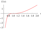
   Figure 1: Potential for massless scalar, $m^{2}=0$, in extremal BTZ: $r_{0}=1$

   

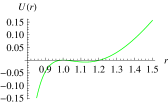
   Figure 2: Potential for massive scalar $0\leq m^{2}=0.5\leq\frac{3}{4}$ in extremal BTZ: $r_{0}=1$

   .

   

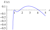
   Figure 3: Potential for massive scalar $\frac{3}{4}<m^{2}=\frac{3.1}{4}\leq\frac{3.33}{4}$ in extremal BTZ: $r_{0}=1$

4. $\frac{3.33}{4}<m^{2}$:

   $$U(r\mapsto 0)\mapsto-\infty,\;\;\;\;U(r=r_{0})=0,\;\;\;\;U(r\mapsto+\infty)\mapsto-\infty.$$ (25)

   and potential has only one extremun in $r_{1}=r_{0}$(Figure(4)).

   

   Figure 4: Potential for massive scalar $\frac{3.33}{4}<m^{2}=1$ in extremal BTZ: $r_{0}=1$

non-Extremal BTZ: In this case, by appropriate choose of the sign of $+$ and $-$ for different regions and solving (4), one finds the ranges of $r^{*}$ as

$$r=[0,r_{-})\;\;\;\;\;\;\;\;\;\;\Leftrightarrow\;\;\;\;\;r^{*}=[0,+\infty),$$ (26)

$$r=(r_{-},r_{+})\;\;\;\;\;\;\;\;\Leftrightarrow\;\;\;\;\;r^{*}=(+\infty,-\infty),$$ (27)

$$r=r_{+},\infty)\;\;\;\;\;\;\;\;\;\Leftrightarrow\;\;\;\;\;r^{*}=(-\infty,0],$$ (28)

The effective potential also reads as

$$U(r)=\frac{(r^{2}-r_{+}^{2})(r^{2}-r_{-}^{2})}{r^{6}}\left((3-4m^{2})r^{4}+(r_{+}^{2}+r_{-}^{2})r^{2}-5r_{+}^{2}r_{-}^{2}\right).$$ (29)

Let us consider only the massless case. It is obvious that $U(r)$, in massless case, has three real positive zeros at $r_{\pm}$ and

$$r_{0}=-\frac{1}{6}(r_{+}^{2}+r_{-}^{2}-\sqrt{r_{+}^{4}+r_{-}^{4}+62r_{+}^{2}r_{-}^{2}}).$$

It is also easy to show that $r_{-}<r_{0}<r_{+}$. We observe that the asymptotic behavior of $U$ is such that $U\rightarrow-\infty$ as $r\rightarrow 0$ and $U\rightarrow+\infty$ as $r\rightarrow+\infty$. Then, we obtain the extremums of $U(r^{*})$ by solving

$$\frac{d}{dr^{*}}U(r^{*})=\frac{(r^{2}-r_{+}^{2})(r^{2}-r_{-}^{2})}{2r^{9}}\times\hskip 170.71652pt$$ (30)

$$\times\left(3r^{8}+(r_{+}^{4}+r_{-}^{4}+4r_{+}^{2}r_{-}^{2})r^{4}-12r_{+}^{2}r_{-}^{2}(r_{+}^{2}+r_{-}^{2})r^{2}+15r_{+}^{4}r_{-}^{4}\right)=0.$$ (31)

Again $r_{+}$ and $r_{-}$ are extremums of $U(r^{*})$. Defining $x=r^{2}$ and considering the general properties of quartic equations, one can prove that there are exactly two other real positive extremas for effective potential. In fact, if $x_{1},x_{2},x_{3}$ and $x_{4}$ be the zeros of

$$3x^{4}+(r_{+}^{4}+r_{-}^{4}+4r_{+}^{2}r_{-}^{2})x^{2}-12r_{+}^{2}r_{-}^{2}(r_{+}^{2}+r_{-}^{2})x+15r_{+}^{4}r_{-}^{4}=0.$$ (32)

they should satisfy

$$x_{1}x_{2}x_{3}x_{4}=15r_{+}^{4}r_{-}^{4}>0$$ (33)

$$\Sigma x_{i}x_{j}x_{k}=12r_{+}^{2}r_{-}^{2}(r_{+}^{2}+r_{-}^{2})>0$$ (34)

$$\Sigma x_{i}x_{j}=r_{+}^{4}+r_{-}^{4}+4r_{+}^{2}r_{-}^{2}>0$$ (35)

$$\Sigma x_{i}=0$$ (36)

For proving the statement, one should recall that if a complex number $z$ be a solution of a polynomial equation then the $\bar{z}$ also is a solution. After all, we can plot the $U(r)$ qualitatively as(Figure(5)).

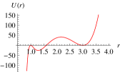
Figure 5: Potential for massless scalar in non-extremal BTZ: $r_{-}=1,r_{+}=3$.

3.2 New Type Black Hole

New Type black hole solution is[4] given by

$$N^{2}(r)=r^{2}+br+c,\;\;\;\;\;\;\;\;\;\;\;R^{2}(r)=r^{2}$$ (37)

$$P^{2}(r)=\frac{1}{r^{2}+br+c}\;\;\;\;\;\;\;\;\;\;\;\;N_{\theta}=0$$ (38)

For non-extremal new type black hole($b^{2}-4ac\neq 0$), one can find

$$r^{*}=\pm\frac{1}{\sqrt{b^{2}-4ac}}\ln{\left(\frac{2ar+b-\sqrt{b2-4ac}}{2ar+b+\sqrt{b2-4ac}}\right)}$$ (39)

and

$$U(r)=\frac{1}{2r^{2}}(ar^{2}+br+c)\left((3a-2m^{2})r^{2}+br-c\right)$$ (40)

Let us consider the extremal case where $b^{2}-4ac=0$ and $r_{+}=r_{-}=r_{0}=-\frac{b}{2a}$. In this case we can find the inverse function $r=f^{-1}(r^{*})$ exactly. In fact, we have

$$r^{*}=\pm\int{\frac{1}{(r-r_{0})^{2}}}=\mp\frac{1}{r-r_{0}}+c_{0},$$ (41)

where $c_{0}$ is an integration constant and $+/-$, in front of the integral, are for interior and exterior regions of horizon respectively. Here, we set $c_{0}=\frac{1}{r_{0}}(1-\theta(r-r_{0}))$ where $\theta(r-r_{0})$ is step function. So, we obtain the domain of changes of $r^{*}$ as

$$r=[0,r_{0})\;\;\;\;\;\;\;\;\;\;\Leftrightarrow\;\;\;\;\;r^{*}=[0,+\infty),$$ (42)

$$r=(r_{0},+\infty)\;\;\;\;\;\Leftrightarrow\;\;\;\;\;r^{*}=(+\infty,0].$$ (43)

Also, we can easily find

$$r=\mp\frac{1}{r^{*}-c_{0}}+r_{0}.$$ (44)

Putting (44) in (40), one obtains $U(r^{*})$. Let us study the asymptotic of $U$, again, in $r$ coordinate. We have different regions due to mass parameter as

1. $3a-2m^{2}\leq 0$:

   $$U(r\mapsto 0)\mapsto-\infty,\;\;\;\;U(r=r_{0})=0,\;\;\;\;U(r\mapsto+\infty)\mapsto-\infty.$$ (45)

   $U(r)$ has only one real positive extremum in $r=r_{0}$(Figure(6)).

   

   Figure 6: Potential for massive scalar in extremal new type B.H: $r_{0}=1,3a-2m^{2}=-1$

2. $0<3a-2m^{2}\leq 3:$

   $$U(r\mapsto 0)\mapsto-\infty,\;\;\;\;U(r=r_{0})=0,\;\;\;\;U(r\mapsto+\infty)\mapsto+\infty.$$ (46)

   and potential has two extremums one in $r_{1}=r_{0}$ and the other in $r_{2}>r_{0}$(Figure(7)).

   

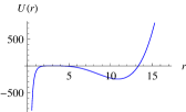
   Figure 7: Potential for massive scalar in extremal new type B.H: $r_{0}=1,3a-2m^{2}=0.5$

3. $3<3a-2m^{2}$:

   $$U(r\mapsto 0)\mapsto-\infty,\;\;\;\;U(r=r_{0})=0,\;\;\;\;U(r\mapsto+\infty)\mapsto+\infty.$$ (47)

   and potential has two extremums one in $r_{1}=r_{0}$ and the other is in $r_{2}<r_{0}$(Figure(8)).

   

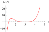
   Figure 8: Potential for massive scalar in extremal new type B.H: $r_{0}=1,3a-2m^{2}=10$ in extremal BTZ: $r_{0}=1$

3.3 Black Hole with Vanishing Horizon

In this section, we study black holes with vanishing horizon in three dimensions. We consider following case where the solution has a null Killing vector[8]. As we will see, the global behavior of this solution, in general, is different from the BTZ and new type solutions. In fact, the effective potential, with a certain condition, has two extremum(one in origin and the other out of origin), otherwise, has only one extremum at origin and so is a monotonic function. A class of such solutions in three dimensional massive gravity is given by[8]

$$R^{2}(r)=l^{2}a_{+}r^{2}+2r+l^{2}d,\;\;\;\;\;\;\;\;\;\;\;N^{2}=\frac{4r^{2}}{l^{2}R^{2}}$$ (48)

$$P^{2}(r)=\frac{l^{2}}{4r^{2}}\;\;\;\;\;\;\;\;\;\;\;\;\;\;\;N_{\theta}=\frac{2r}{lR^{2}}$$ (49)

where $l,m$ are parameters in three dimensional massive gravity and are related to cosmological constant and mass parameter of the action and $a_{+},d$ are some integration constants. Having regular solution forces us $m^{2}l^{2}=17/2$ and $a_{+}>0,d>0$. Defining $l^{2}a_{+}r=x$ and $l^{4}da_{+}=s$ one obtains for $r^{*}$ as

$$r^{*}=+\frac{l^{5}a_{+}^{\frac{3}{2}}}{4}\int{\frac{\sqrt{x^{2}+2x+s}}{x^{2}}dx}$$ (50)

Here one can find the exact result of the integral (50). By the above choosing of $+$ in front of the integral we will have

$$r=[0,+\infty)\;\;\;\;\;\;\;\;\;\;\Leftrightarrow\;\;\;\;\;r^{*}=(-\infty,+\infty).$$ (51)

Then, we obtain the potential for massless scalar as

$$U(r)=\frac{4x^{3}}{a_{+}l^{6}(x^{2}+2x+s)^{3}}\left(x^{3}+6x^{2}+(6s+3)x+4s\right)$$ (52)

It is easy to see that $U(r)\geq 0$ for $r\geq 0$ and

$$U(r\rightarrow 0)\rightarrow 0,\;\;\;\;\;\;\;\;U(r\rightarrow+\infty)\rightarrow\frac{4}{a_{+}l^{6}}$$ (53)

Also, for derivative of potential $\frac{d}{dr^{*}}U(r^{*})$, one can obtain

$$\frac{d}{dr^{*}}U(r^{*})\varpropto\frac{x^{4}}{R^{9}}\left((3-s)x^{3}+(5s+1)x^{2}+2s(2s+1)x+2s^{2}\right)$$ (54)

As we can see $x=0$ and roots of

$$(3-s)x^{3}+(5s+1)x^{2}+2s(2s+1)x+2s^{2}=0$$ (55)

are the extremum of $U$. Here there are two regions in term of $s$.

• $0\leq s\leq 3$: In this case, one can easily see that equation (55) has no real positive solution because all terms are positive. So the general behavior of $U$ can be plotted as blue curve in(Figure(9)).

• $3<s$: Here, by considering the general properties of cubic equations

  $$x_{1}x_{2}x_{3}=-\frac{2s^{2}}{3-s}>0$$ (56)

  $$\Sigma x_{i}x_{j}=\frac{2s(2s+1)}{3-s}<0$$ (57)

  $$\Sigma x_{i}=-\frac{5s+1}{3-s}>0$$ (58)

  one can prove that (55) has only one real positive solution. So, one may plot the effective potential as red curve in(Figure(9)).

  

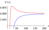
  Figure 9: Potential for massless scalar in black hole with no horizon: the blue curve is for $0<s\leq 3$ and the red curve is for $s>3$.

4 Fermions in $3-$D Black Hole Background

In this section, we study the potential seen by a Tortoise observer for a spinor field. Spinor field representation in three dimension has two components and the coupled equation of motion for these fields is given by Dirac equation in curved background as[2]

$$(-i\gamma^{a}e_{a}^{\mu}D_{\mu}+m)\Psi(t,\theta,r)=0,$$ (59)

where the covariant derivative is $D_{\mu}=\partial_{\mu}-\frac{i}{4}\eta_{ac}\omega^{c}_{b\mu}\sigma^{ab}$ and $\sigma^{ab}=\frac{i}{2}[\gamma^{a},\gamma^{b}]$. $\omega^{c}_{b\mu}$ are spin connection and are defined by veilbeins and Christoffel coefficients as $\omega^{c}_{b\mu}=e^{c}_{\nu}\partial_{\mu}e^{\nu}_{b}+e^{c}_{\nu}e^{\sigma}_{b}\Gamma^{\nu}_{\sigma\mu}$. For the background (7), one can obtain non-zero veilbains as

$$e^{t}_{0}=-\frac{1}{N},\;\;\;\;\;e^{\theta}_{0}=\frac{N_{\theta}}{N},\;\;\;\;\;e^{r}_{1}=\frac{1}{P},\;\;\;\;\;e^{\theta}_{2}=\frac{1}{R},$$ (60)

and so the covariant derivatives take the following forms

$$D_{t}=\partial_{t},\;\;\;\;\;\;D_{\theta}=\partial_{\theta},$$ (61)

$$D_{r}=\partial_{r}-\frac{i}{8NR}\partial_{r}(R^{2}N_{\theta})\sigma_{1}$$ (62)

By rewriting two dimensional spinor field $\Psi(t,\theta,r)$ as

$$\Psi(t,\theta,r)=e^{-i(\omega t-k\theta)}\begin{pmatrix}\phi^{+}\\ \phi^{-}\end{pmatrix}$$ (63)

one finds

$${\cal{M}}\phi^{+}+{\cal{N}}\phi^{-}+\partial_{r}\phi^{-}=0$$ (64)

$$\bar{\cal{M}}\phi^{-}+\bar{\cal{N}}\phi^{+}+\partial_{r}\phi^{+}=0$$ (65)

where

$${\cal{N}}=i\frac{P}{N}(\omega+kN_{\theta})$$ (66)

$${\cal{M}}=\frac{1}{8NR}\partial_{r}(R^{2}N_{\theta})+P(m+i\frac{k}{R}),$$ (67)

and one may obtain following tow decoupled equations for $\phi^{+}$ and $\phi^{-}$

$$\partial^{2}_{r}\phi^{+}+(-\frac{\partial_{r}{\bar{\cal{M}}}}{\bar{\cal{M}}})\partial_{r}\phi^{+}+(|{\cal{N}}|^{2}-|{\cal{M}}|^{2}+\bar{\cal{M}}\partial_{r}(\frac{\bar{\cal{N}}}{\bar{\cal{M}}}))\phi^{+}=0,$$ (68)

$$\partial^{2}_{r}\phi^{-}+(-\frac{\partial_{r}{{\cal{M}}}}{{\cal{M}}})\partial_{r}\phi^{-}+(|{\cal{N}}|^{2}-|{\cal{M}}|^{2}+{\cal{M}}\partial_{r}(\frac{{\cal{N}}}{{\cal{M}}}))\phi^{-}=0$$ (69)

Note that the coefficient of $\omega^{2}$ again is $\frac{P^{2}}{N^{2}}$. This is just from the fact that spinor equation is a linearization of Schrodinger equation. So, for evaluating the effective potential of spinors we have for $\phi^{+}$

$$A^{+}(m,\omega,k;r)=-\frac{\partial_{r}{\bar{\cal{M}}}}{\bar{\cal{M}}}$$ (70)

$$B^{+}(m,\omega,k;r)=\frac{P^{2}}{N^{2}}(2\omega kN_{\theta}+k^{2}N^{2}_{\theta})-|{\cal{M}}|^{2}+\bar{\cal{M}}\partial_{r}(\frac{\bar{\cal{N}}}{\bar{\cal{M}}})$$ (71)

and simply $A^{-}=\bar{A}^{+},B^{-}=\bar{B}^{+}$ for $\phi^{-}$. Thus, we obtain

$$U(r)=\hskip 540.60236pt$$ (72)

$$\frac{N^{2}}{2P^{2}}\left(\frac{P^{\prime\prime}}{P}-\frac{N^{\prime\prime}}{N}-\frac{\bar{\cal{M^{\prime\prime}}}}{\bar{\cal{M}}}-\frac{3}{2}(\frac{P^{\prime}}{P})^{2}+\frac{1}{2}(\frac{N^{\prime}}{N})^{2}+\frac{3}{2}(\frac{\bar{\cal{M^{\prime}}}}{\bar{\cal{M}}})^{2}+(\frac{P^{\prime}}{P})(\frac{N^{\prime}}{N})-2B\right)(21)\hskip 170.71652pt$$ (73)

for $\phi^{+}$ and $\bar{U}$ for $\phi^{-}$. Here, we do not want to study the potential with details and only present some comments for two cases.

• BTZ and New type Black Holes: We see that for BTZ and new type black holes $\partial_{r}(R^{2}N_{\theta})=0$. Then, massless spinors components $\phi^{+}$ and $\phi^{-}$ have the same potential but only the zero of them have decoupled dynamics from each other. Beside of these, for massless zero mode we obtain a harmonic oscillator-like potential for two components.

  In massive case, two components always have coupled dynamics and only stationary zero modes they have the same potential.

• Black Holes with No Horizon: But, in black hole with no horizon where we have $\partial_{r}(R^{2}N_{\theta})=2/l\neq 0$, even the stationary massless zero modes do not have decoupled dynamics. They also do not have the same potential due to the fact that ${\cal{N}}$ is imaginary unless for stationary zero mode where. Especially for stationary massless zero mode they have an oscillator-like potential.

5 Conclusion

In this note, we study the fields dynamics in Tortoise frame. In this frame, by defining new coordinate $r^{*}(r)$ and an unknown auxiliary field $\theta(r)$ the equation of motion of a scalar field can be written as Schrodinger-like form. Using this change of variables we can obtain two conditions for $r^{*}$ and $\theta$ and then obtain a general form for effective potential. Then, we apply this formula for scalar and fermionic fields in some black hole backgrounds in three dimension such as BTZ black holes, new type black holes and black holes with no horizon and find the potential. Although, in general, we can not find the inverse function $r(r^{*})$ but by some simple calculations, We study the asymptotic behavior of potential at infinity, horizons and origin and also find the extremum of that.

Interestingly, we find that the asymptotic of potential in BTZ and new type solution is completely different from that of vanishing horizon solution. In fact, potential for vanishing horizon goes to a fixed number at infinity but for BTZ and new type black hole background we have an infinite barrier at infinity.

References

- [1] J. M. Maldacena, “The Large N limit of superconformal field theories and supergravity,” Adv. Theor. Math. Phys. 2, 231 (1998) [Int. J. Theor. Phys. 38, 1113 (1999)] [arXiv:hep-th/9711200].
- [2] C. M. Harris and P. Kanti, JHEP 0310, 014 (2003) [arXiv:hep-ph/0309054]. E. Jung, S. Kim and D. K. Park, JHEP 0409, 005 (2004) [arXiv:hep-th/0406117]. J. J. Oh and W. Kim, JHEP 0901, 067 (2009) [arXiv:0811.2632 [hep-th]]. H. C. Kao and W. Y. Wen, JHEP 0909, 102 (2009) [arXiv:0907.5555 [hep-th]]. S. K. Chakrabarti, P. R. Giri and K. S. Gupta, Phys. Lett. B 680, 500 (2009) [arXiv:0903.1537 [hep-th]].
- [3] J. J. Oh and W. Kim, Eur. Phys. J. C 65, 275 (2010) [arXiv:0904.0085 [hep-th]]. C. Campuzano, P. Gonzalez, E. Rojas and J. Saavedra, JHEP 1006, 103 (2010) [arXiv:1003.2753 [gr-qc]]. JHEP 1008, 081 (2010) [arXiv:1006.4468 [hep-th]]. R. Li and J. R. Ren, Phys. Rev. D 83, 064024 (2011) [arXiv:1008.3239 [hep-th]]. C. Campuzano, P. Gonzalez, E. Rojas and J. Saavedra, JHEP 1006, 103 (2010) [arXiv:1003.2753 [gr-qc]]. R. Li, S. Li and J. R. Ren, Class. Quant. Grav. 27, 155011 (2010) [arXiv:1005.3615 [hep-th]]. R. Fareghbal, Phys. Lett. B 694, 138 (2010) [arXiv:1006.4034 [hep-th]]. Y. Kwon, S. Nam, J. D. Park and S. H. Yi, arXiv:1102.0138 [hep-th]. W. Yao, S. Chen and J. Jing, arXiv:1101.0042 [gr-qc]. R. A. Konoplya and A. Zhidenko, arXiv:1102.4014 [gr-qc].
- [4] E. A. Bergshoeff, O. Hohm and P. K. Townsend, Phys. Rev. Lett. 102, 201301 (2009) [arXiv:0901.1766 [hep-th]]. E. A. Bergshoeff, O. Hohm and P. K. Townsend, Phys. Rev. D 79, 124042 (2009) [arXiv:0905.1259 [hep-th]]. E. A. Bergshoeff, O. Hohm and P. K. Townsend, Annals Phys. 325, 1118 (2010) [arXiv:0911.3061 [hep-th]]. R. Andringa, E. A. Bergshoeff, M. de Roo, O. Hohm, E. Sezgin and P. K. Townsend, Class. Quant. Grav. 27, 025010 (2010) [arXiv:0907.4658 [hep-th]]. E. Bergshoeff, O. Hohm and P. Townsend, J. Phys. Conf. Ser. 229, 012005 (2010) [arXiv:0912.2944 [hep-th]]. H. R. Afshar, M. Alishahiha and A. Naseh, Phys. Rev. D 81, 044029 (2010) [arXiv:0910.4350 [hep-th]].
- [5] K. A. Moussa, G. Clement and C. Leygnac, Class. Quant. Grav. 20, L277 (2003) [arXiv:gr-qc/0303042]. A. Garbarz, G. Giribet and Y. Vasquez, Phys. Rev. D 79, 044036 (2009) [arXiv:0811.4464 [hep-th]]. K. Skenderis, M. Taylor and B. C. van Rees, JHEP 0909, 045 (2009) [arXiv:0906.4926 [hep-th]]. G. Clement, Class. Quant. Grav. 26, 105015 (2009) [arXiv:0902.4634 [hep-th]]. A. Sinha, JHEP 1006, 061 (2010) [arXiv:1003.0683 [hep-th]]. I. Gullu, T. Cagri Sisman and B. Tekin, Class. Quant. Grav. 27, 162001 (2010) [arXiv:1003.3935 [hep-th]]. M. Alishahiha, A. Naseh and H. Soltanpanahi, Phys. Rev. D 82, 024042 (2010) [arXiv:1006.1757 [hep-th]]. A. Ghodsi and M. Moghadassi, Phys. Lett. B 695, 359 (2011) [arXiv:1007.4323 [hep-th]]. S. Nam, J. D. Park and S. H. Yi, JHEP 1007, 058 (2010) [arXiv:1005.1619 [hep-th]].
- [6] D. Anninos, W. Li, M. Padi, W. Song and A. Strominger, JHEP 0903, 130 (2009) [arXiv:0807.3040 [hep-th]]. B. Chen and B. Ning, Phys. Rev. D 82, 124027 (2010) [arXiv:1005.4175 [hep-th]]. E. Tonni, JHEP 1008, 070 (2010) [arXiv:1006.3489 [hep-th]].
- [7] M. Banados, C. Teitelboim and J. Zanelli, “The Black hole in three-dimensional space-time,” Phys. Rev. Lett. 69, 1849 (1992) [arXiv:hep-th/9204099].
- [8] G. Clement, “Black holes with a null Killing vector in new massive gravity in three dimensions,” Class. Quant. Grav. 26, 165002 (2009) [arXiv:0905.0553 [hep-th]].