Fast, large volume, GPU enabled simulations for the $\mn@boldsymbol{\mathrm{Ly}\alpha{}}$ forest: power spectrum forecasts for baryon acoustic oscillation experiments

Abstract

High redshift measurements of the baryonic acoustic oscillation scale (BAO) from large Ly$\alpha$ forest surveys represent the next frontier of dark energy studies. As part of this effort, efficient simulations of the BAO signature from the Ly$\alpha$ forest will be required. We construct a model for producing fast, large volume simulations of the Ly$\alpha$ forest for this purpose. Utilising a calibrated semi-analytic approach, we are able to run very large simulations in 1 Gpc³ volumes which fully resolve the Jeans scale in less than a day on a desktop PC using a GPU enabled version of our code. The Ly$\alpha$ forest spectra extracted from our semi-analytical simulations are in excellent agreement with those obtained from a fully hydrodynamical reference simulation. Furthermore, we find our simulated data are in broad agreement with observational measurements of the flux probability distribution and 1D flux power spectrum. We are able to correctly recover the input BAO scale from the 3D Ly$\alpha$ flux power spectrum measured from our simulated data, and estimate that a BOSS-like $10^{4}\rm~{}deg^{2}$ survey with $\sim 15$ background sources per square degree and a signal-to-noise of $\sim 5$ per pixel should achieve a measurement of the BAO scale to within $\sim$1.4 per cent. We also use our simulations to provide simple power-law expressions for estimating the fractional error on the BAO scale on varying the signal-to-noise and the number density of background sources. The speed and flexibility of our approach is well suited for exploring parameter space and the impact of observational and astrophysical systematics on the recovery of the BAO signature from forthcoming large scale spectroscopic surveys.

1 Introduction

The Ly$\alpha$ forest is the series of absorption lines arising from the resonant scattering of redshifted Ly$\alpha$ photons emitted from a background source by the intervening neutral hydrogen in the intergalactic medium (Rauch, 1998). The neutral hydrogen is in photo-ionisation equilibrium with the ionising background produced by the integrated emission from galaxies and quasars (e.g. Meiksin, 2009). Numerical simulations and semi-analytical models have demonstrated that the Ly$\alpha$ forest is a valuable probe of the underlying matter density field in the intergalactic medium (IGM), tracing the so-called “cosmic web” of large scale structure (Cen et al., 1994; Hernquist et al., 1996; Bi & Davidsen, 1997; Theuns et al., 1998). The measurement of fluctuations in the transmitted Ly$\alpha$ flux in samples of quasar spectra (McDonald et al., 2000; Croft et al., 2002; Kim et al., 2004), combined with a suitable model to connect the observed flux to the underlying matter distribution, thus enable the matter power spectrum (PS) to be inferred on small scales along the line-of-sight (Croft et al., 2002; Viel et al., 2004; McDonald et al., 2005).

In recent years, it has been proposed that the Ly$\alpha$ forest of absorption lines may also be used to detect the signature of baryonic acoustic oscillations (BAO) in the large scale structure of the IGM (e.g. McDonald & Eisenstein, 2007). BAOs provide a standard ruler which may be used to examine the geometry of the Universe and the nature of dark energy, and are already observed in the Cosmic Microwave Background (CMB) at $z\sim 1100$ and the clustering of galaxies at low redshift (Eisenstein et al., 2005; Cole et al., 2005; Hütsi, 2006; Blake et al., 2007; Padmanabhan et al., 2007; Percival et al., 2007, 2010; Beutler et al., 2011; Blake et al., 2011). The characteristic BAO signal is spatially correlated on scales of order $\sim 150$ comoving Mpc; large survey volumes are therefore required to provide adequate statistics for the detection of this scale. Existing low redshift studies are subject to a degeneracy between the space-time curvature $\Omega_{k}$ and an evolving dark energy equation of state (Zhan et al., 2005). Studying BAO at higher redshift can help alleviate this difficulty. However, the extension of galaxy surveys to higher redshifts becomes increasingly expensive because of the significant telescope resources required to observe a sufficient number of (fainter) galaxies.

An alternate measurement of large scale structure at $z\simeq 2-3$ is provided by the Ly$\alpha$ forest. There are several advantages to using the Ly$\alpha$ forest as a probe of BAO. At higher redshifts the evolution of $\Omega_{k}$ and dark energy differ ($\Omega_{k}$ evolves as $\propto(1+z)^{2}$, whereas dark energy is expected to evolve more slowly with redshift) allowing one to break this degeneracy and to obtain constraints on the dark energy equation of state at this epoch. Furthermore, the detection of suitable background sources becomes significantly easier due to the peak in quasar number density observed at $z\simeq 2.2$ (Richards et al., 2006). McDonald & Eisenstein (2007) demonstrated that low to medium signal-to-noise (S/N) spectra of a large number of quasars with sufficient density per square degree could be used to detect the BAO signal with the Ly$\alpha$ forest. As an example, these authors estimated that the BAO scale could be measured in a 2000 square degree survey with 40 quasars per square degree. The BAO signal may then be statistically extracted from such a sample via either the correlation function (measured as a characteristic peak) or the power spectrum (measured as a characteristic oscillation period). More recently McQuinn & White (2011) demonstrated the sensitivity of future Ly$\alpha$ forest surveys to the flux correlation function, and investigated the optimal survey configuration for estimating the Ly$\alpha$ forest correlations including the use of galaxies as background sources to boost the Ly$\alpha$ forest survey sensitivity. These authors also estimate the sensitivity of a future BAO measurement to the systematics associated with Ly$\alpha$ forest surveys.

In anticipation of the necessary large volume Ly$\alpha$ forest surveys such as the Baryon Oscillation Spectroscopic Survey (BOSS; Schlegel et al., 2009; Slosar et al., 2011), simulation work has also been carried out to construct synthetic Ly$\alpha$ forest spectra for use in constructing mock surveys. Recently, large volume, high resolution dark matter (DM) N-body simulations have been performed by White et al. (2010) and Slosar et al. (2009), while Norman et al. (2009) have presented fully hydrodynamical simulations in slightly smaller volumes for this purpose. In this work we outline a method for producing fast (i.e. less than one day), similarly large volume, high resolution simulations using a single desktop PC with a graphics processing unit (GPU). Our approach, which is based on widely used semi-analytical models for the Ly$\alpha$ forest (Bi, 1993; Reisenegger & Miralda-Escude, 1995; Gnedin & Hui, 1996; Bi & Davidsen, 1997; Hui et al., 1997; Gnedin & Hui, 1998; Choudhury et al., 2001; Matarrese & Mohayaee, 2002; Viel et al., 2002a, b), does not capture the mildly non-linear effects of the Ly$\alpha$ forest modelled in the N-body and hydrodynamical simulations. Nevertheless, this method is well suited for studying the statistics of Ly$\alpha$ forest absorption on large scales, where the assumption of linear evolution is a reasonable approximation. Our approach is therefore complimentary to more accurate but very expensive numerical simulations. We note another semi-analytical approach for studying the BAO in the Ly$\alpha$ forest has also been recently presented by Kitaura et al. (2010).

This paper is organised as follows. In Section 2, we provide a summary of the semi-analytical model and the method used for generating our synthetic Ly$\alpha$ forest spectra. In Section 3 we compare the semi-analytical density and velocity fields to a fully hydrodynamical simulation. In Section 4 we describe the simulations used in this work in more detail. In Section 5 we test our model by comparison to a fully hydrodynamical simulation and a selection of observational data, and in Section 6 we extract the BAO signature from a mock Ly$\alpha$ BAO survey and compare our approach to other recently published work. In Section 7 we provide scaling relations for the fractional error on the recovery of the BAO scale for Ly$\alpha$ forest BAO surveys. Finally, in Section 8 we finish with our closing remarks. An appendix detailing the performance and implementation of our GPU enabled code is included at the end of the paper.

2 Semi-Analytical Model for the IGM

Many approximate techniques have been proposed for modelling the mildly non-linear, low column density IGM from an initial dark matter distribution. Approaches taken include the lognormal method (Coles & Jones, 1991) applied to the linear DM distribution to mimic non-linear behaviour (Bi, 1993; Bi & Davidsen, 1997; Choudhury et al., 2001), the rank-ordered mapping of linear to non-linear densities using a calibration hydrodynamical simulation (Viel et al., 2002b) or using the Zel’dovich approximation (Zel’Dovich, 1970) to generate the DM distribution. Many of these models also subsequently smooth the initial DM density field on a scale related to the Jeans length in the low density IGM, accounting for the effect of gas pressure on the baryon distribution on small scales (Reisenegger & Miralda-Escude, 1995; Gnedin & Hui, 1996, 1998; Hui et al., 1997; Matarrese & Mohayaee, 2002; Viel et al., 2002a).

In this work we follow Viel et al. (2002b), who investigated various approaches for producing more accurate models for the gas density distribution using semi-analytical models. These authors found they could better mimic the non-linear DM distribution by taking the DM density probability distribution function (PDF) from a linear simulation and performing a rank-ordered mapping to the corresponding distribution obtained from a hydrodynamical simulation. We adopt a similar approach here, and use a hydrodynamical simulation to calibrate the one point distribution for the density field. This ensures we obtain accurate one and two point statistics for most of the absorption in the resulting Ly$\alpha$ spectra. However, as noted by Viel et al. (2002b) the two point statistics for regions of strong absorption with $F=e^{-\tau}<0.1$, where non-linear effects are important, will not be properly captured by this model. In this paper, we demonstrate this limitation will not present a serious impediment to extracting the BAO signal on large scales from our simulated data. We stress, however, that our semi-analytical simulations are based on linear theory and they do not include large scale non-linear evolution and BAO damping as described in the detailed N-body work of Seo & Eisenstein (2007). Rather, our models can be used to address the non-gravitational issues associated with the Ly$\alpha$ forest, and will need to be coupled with N-body studies of the gravitational evolution of the BAO in order to make detailed comparisons with real data.

We use model L3 of Bolton et al. (2010) as our calibration hydrodynamical simulation, with a snapshot at $z=2.976$ generated using the parallel Tree-SPH code GADGET-3 (Springel, 2005). This simulation assumes a $\Lambda$CDM cosmology with, $h=0.72$, $\Omega_{\rm{m}}=0.26$, $\Omega_{\Lambda}=0.74$, $\Omega_{\rm{b}}=0.0444$, $n_{\rm{s}}=0.96$ and $\sigma_{8}=0.8$. The calibration simulation has a box size of 40 $h^{-1}$ Mpc and contains $2\times 512^{3}$ gas and DM particles, yielding a gas particle mass resolution of $5.9\times 10^{6}h^{-1}M_{\odot}$. Importantly, this particular box size and mass resolution is sufficient for resolving the gas densities responsible for the Ly$\alpha$ forest at $z\simeq 3$ (Bolton & Becker, 2009). We note that in this work we assume a constant redshift of $z=3$ for our simulations. The accuracy to which the BAO scale can be recovered is redshift dependent and as such we would expect our results to differ slightly across the redshift range of $z=2-3$.

2.1 Generation of the density field

We begin by generating a linear DM density field in Fourier space within a cubic simulation volume according to the transfer function of Eisenstein & Hu (1998). The density field is then linearly evolved using the linear growth factor $D_{+}(z)$ to the redshift of interest. Following Bi & Davidsen (1997), we account for the effect of gas pressure on the baryons by smoothing the linear DM density field with the kernel

$$\delta_{\rm{b}}(\mn@boldsymbol{k},z)=\frac{\delta_{\rm{DM}}(\mn@boldsymbol{k},z)}{1+k^{2}/k^{2}_{F}(z)},$$ (1)

where $k_{F}$ is the filtering scale, which is related to the comoving Jeans scale $k_{J}$ via $k_{F}=\epsilon k_{J}$. The comoving Jeans scale is given by

$$k_{J}=H_{0}\left[\frac{3\mu m_{\rm{p}}\Omega_{\rm{m}}(1+z)}{2\gamma k_{\rm{B}}T(z)}\right]^{1/2},$$ (2)

where $\mu$ is the reduced mass and $T(z)$ is the gas temperature. The smoothing scale $k_{F}$ is a free parameter in the simulations, and effectively accounts for the finite delay between heating and the subsequent pressure response of the gas, which is dependent on the specific reionisation history (Gnedin & Hui, 1998; Desjacques & Nusser, 2005). In this work we choose $k_{F}=6.5$ Mpc^-1, which we find provides good agreement with spectra extracted from our calibration hydrodynamical simulation and the observational data (see Section 5). In Section 3 we compare the generated linear density field and the corresponding non-linear rank-ordered density field to the calibration hydrodynamical simulation using the three dimensional matter power spectrum.

2.2 Generation of the velocity field

In addition to the density field, the Ly$\alpha$ forest is also sensitive to the peculiar velocity field. We generate the linear peculiar velocity field, based on our linear DM density field, using the following expression,

$$\mn@boldsymbol{v}_{IGM}(\mn@boldsymbol{k},z)=E_{+}(z)i\mn@boldsymbol{k}/k^{2}\delta_{\rm{DM}}(\mn@boldsymbol{k}),$$ (3)

where $\mn@boldsymbol{v}_{IGM}$ is expressed relative to the comoving wavenumber $\mn@boldsymbol{k}$, $E_{+}(z)=H(z)f(\Omega_{\rm{m}},\Omega_{\rm{\Lambda}})D_{+}(z)/(1+z)$ and $f(\Omega_{\rm{m}},\Omega_{\rm{\Lambda}})=-\rm{dln}D_{+}(z)/\rm{dln}(1+z)$. We compare the linear peculiar velocities generated from Equation 3 with the peculiar velocities in the calibration hydrodynamical simulation in more detail Section 3.

2.3 Generation of $\mn@boldsymbol{\mathrm{Ly}\alpha{}}$ forest spectra

The calibrated baryonic density and peculiar velocity fields are next used to generate the synthetic Ly$\alpha$ forest spectra. We use the approach outlined in Hui et al. (1997), assuming that the neutral hydrogen in the ionised IGM is in photo-ionisation equilibrium; this should be a reasonable approximation at $z\simeq 3$. The proper number density of neutral hydrogen in the IGM is

$$n_{\rm{HI}}(\mn@boldsymbol{x},z) = 7.24\times 10^{-6}\bar{n}_{\rm{H}}(z)\left(\frac{T}{10^{4}K}\right)^{-0.7}\left(\frac{\Omega_{\rm{b}}h^{2}}{0.024}\right)$$ (4)

$$\times\left(\frac{1}{\Gamma_{-12}}\right)[1+\delta_{\rm{b}}(\mn@boldsymbol{x},z)]^{2}\left(\frac{1+z}{4}\right)^{3},$$

where $\bar{n}_{\rm{H}}$ is the proper mean density of neutral hydrogen, $\Gamma_{-12}$ is the hydrogen photo-ionisation rate in units of $10^{-12}\rm\,s^{-1}$ and $\delta_{\rm{b}}$ is the baryonic overdensity and is a function of the comoving position $\mn@boldsymbol{x}$. We take the case-A recombination rate of neutral hydrogen to be $4.17\times 10^{-13}\left(\frac{T}{10^{4}K}\right)^{-0.7}\rm\,cm{{}^{3}}\,s^{-1}$. The temperature of the low density IGM, $\delta+1\leq 10$, is then modelled assuming a power-law temperature-density relation

$$T=T_{0}(1+\delta_{\rm{b}})^{\gamma-1},$$ (5)

where $\gamma$ is the polytropic index describing the slope of the temperature-density relation. This relation is expected to arise following reionisation due to the interplay between photo-heating and adiabatic cooling, where typically $1<\gamma<1.6$ (Hui et al., 1997; Valageas et al., 2002). However, at densities $\delta+1>10$, radiative cooling becomes more efficient and the power-law temperature density relation is no longer a good approximation. We therefore employ a pivot point at $\delta+1=10$, below which the typical temperature-density relation still holds, but above which we set the temperature to be constant, such that $T(\delta+1>10)=T(\delta+1=10)$. Note, however, shock heating will introduce some scatter into this relation. Furthermore, HeII reionisation, which is expected to end around $z\simeq 3$, may also produce a relationship between temperature and density which is more complicated than this tight power-law (Bolton et al., 2009; McQuinn et al., 2009). There is also some observational evidence for $\gamma<1$ (i.e. an inverted temperature-density relation, Viel et al. 2009), although it appears difficult to achieve this via heating during HeII reionisation alone (Bolton et al., 2009; McQuinn et al., 2009). However, we defer the discussion of such possible systematic uncertainties to a future study.

We next generate the transmitted Ly$\alpha$ flux along the line-of-sight for our synthetic Ly$\alpha$ forest spectra using the relation $F=e^{-\tau}$, where $\tau$ is the Ly$\alpha$ optical depth. The optical depth of the synthetic Ly$\alpha$ spectra is computed using (e.g. Theuns et al., 1998)

$$\tau_{\rm{\alpha}}(i)=\frac{c\sigma_{\alpha}\delta R}{\pi^{1/2}}\sum_{j=1}^{N}\frac{n_{\rm{HI}}}{b_{\rm{HI}}(j)}\exp\left[-\left(\frac{v_{\rm{H}}(i)-u(j)}{b_{\rm{HI}}(j)}\right)^{2}\right],$$ (6)

where $i$ and $j$ denote pixels along the line of sight through the simulation volume, $\delta R$ is the pixel width in proper coordinates, $\sigma_{\alpha}=4.48\times 10^{-18}\,\rm{cm}^{2}$ is the scattering cross-section for $\mathrm{Ly}\alpha$ photons, $b_{\rm{HI}}=\left(\frac{2k_{\rm{B}}T}{m_{\rm{H}}}\right)^{1/2}$ is the Doppler parameter describing the thermal width of the line profiles, $v_{H}$ is the Hubble velocity and $u(j)$ is the total velocity given by the summation of the Hubble flow and the peculiar velocity along the line of sight, $u(j)=v_{\rm{H}}(j)+v_{\rm{pec}}(j)$.

Finally, once we have our optical depth along the line of sight, we renormalise the optical depths of all of our spectra to match the observed mean flux of the Ly$\alpha$ forest at $z\simeq 3$. We define the transmitted flux as $\langle{F}\rangle=\langle e^{-A\tau}\rangle$, where $A$ is a normalisation constant to be solved for. This modification is equivalent to rescaling the HI photo-ionisation rate produced by the UV background. We solve for $A$ by summation over all generated spectra and iterate $A$ until the mean transmitted flux from the simulated spectra matches the observationally measured value. We match our mean transmitted flux to that observed by Kim et al. (2007), corresponding to a mean transmitted flux of $\langle{F}\rangle=0.72$ or an effective optical depth of $\tau_{\rm{eff}}=0.329$ at $z=3$. Lastly, we note that in the generation of our Ly$\alpha$ spectra, we do not include the redshift evolution of the effective optical depth along individual lines-of-sight. The effect of metal absorption lines and the damping wings originating from high column density absorption systems are also excluded.

3 Semi-Analytic model performance

Before comparing the Ly$\alpha$ forest simulations used in this work with observations, we first verify the performance of our rank-ordered semi-analytic model. Firstly we investigate the effect that rank-ordered mapping of the linear density field has on the matter power spectrum, and secondly, we check that our linear peculiar velocity field produces a reasonable description of the peculiar velocity field when compared to hydrodynamical simulations.

Figure 1: The dimensionless dark matter PS of our 40 $h^{-1}$ Mpc, 512³ semi-analytical simulation before (dot-dashed) and after (dotted) the rank-ordered mapping of the linear density field with our calibration hydrodynamical simulation. For comparison we also show the theoretical linear input PS (solid) and the dark matter PS of the calibration hydrodynamical simulation (dashed).

3.1 Matter power spectrum

In Figure 1, we illustrate the effect of the rank-ordering procedure on the linear dark matter density field by comparing the dimensionless dark matter PS from our semi-analytic simulations to the dark matter PS from the calibration hydrodynamical simulation. We find that the rank-ordered linear matter power spectrum correctly recovers the large scale behaviour when compared to the non-linear dark matter PS from the hydrodynamical simulations. For smaller spatial scales, the non-linear density from the rank-ordered method underpredicts the correct non-linear behaviour. However underproducing the small-scale power will have no significant effect on the BAO scale. Thus, provided we are able to maintain roughly the same spatial resolution in our large-scale simulations as in our calibration simulation, the rank-ordered mapping procedure will perform well at reproducing the correct large-scale behaviour required for accurately simulating the recovery of the BAO scale.

Figure 2: The linear peculiar velocity PDF’s of our 40 $h^{-1}$ Mpc, 512³ semi-analytical simulation. From left to right are the peculiar velocity PDF’s in the x, y and z directions of our simulation (dashed) and the calibration hydrodynamical simulation (solid). The linear peculiar velocity field matches reasonably well in the low density regions which have smaller peculiar velocities. However, the semi-analytical model does not produce the larger (rarer) peculiar velocities expected in non-linear, overdense regions.

3.2 Peculiar velocities

As discussed in the previous section, we also produce the linear peculiar velocity field prior to the rank-ordered mapping of the density field. In Figure 2 we compare the resulting linear peculiar velocity PDFs to those from the hydrodynamical simulation. We find the linear peculiar velocity field to be isotropic, and that the velocities from our simulations match quite well in the low density regions. However as expected, higher density regions with larger (but rarer) peculiar velocities (which correspond to regions of infall in the hydrodynamical simulation) are not correctly captured in this model.

Figure 3: Example synthetic Ly$\alpha$ forest spectrum generated from our $1\rm\,Gpc^{3}$ simulation with 4096³ pixels. Upper panel: The transmitted flux along the line-of-sight predicted by the simulation. Middle panel: The same spectrum after convolution with a Gaussian instrument profile with FWHM$=224\rm\,km\,s^{-1}$. Lower panel: The fully processed spectrum, resampled onto pixels of width $\sim 1\,$Å with Gaussian distributed noise corresponding to a signal-to-noise of $5$ per pixel. This spectrum is representative of the mock data set we use to recover the BAO signal from the Ly$\alpha$ forest. Note that the redshift evolution of the effective optical depth along the line-of-sight is not included in this model.

4 $\mn@boldsymbol{\mathrm{Ly}\alpha{}}$ forest simulations

We construct two different Ly$\alpha$ forest simulations in this work; a high resolution simulation for comparison to our reference hydrodynamical simulation, and a low resolution, large volume simulation for recovery of the BAO signature. Both models are compared to published measurements of the Ly$\alpha$ flux probability distribution function (PDF) and the 1D flux power spectrum (PS). In both simulations we assume a temperature-density relation with $\gamma=1.3$ and we set the temperature $T_{0}=1.7\times 10^{4}~{}$K, broadly consistent with the observational constraints on the IGM thermal state at $z=3$ (Schaye et al., 2000; Lidz et al., 2010; Becker et al., 2011).

4.1 High resolution simulations

In our high resolution model, we simulate a 40 $h^{-1}$ Mpc simulation box, containing $512^{3}$ pixels. The box size and resolution are chosen to mimic our calibration GADGET-3 hydrodynamical simulation, although we note that the resolution comparison will not be exact due to the spatially adaptive resolution of GADGET-3. In order to compare our simulated Ly$\alpha$ forest spectra to observed high resolution data, we must also process our simulated spectra to mimic the properties of the data. We convolve the spectra with a Gaussian with a FWHM $=7\rm~{}km~{}s^{-1}$, and resample our spectra onto 0.05 Å bins. We finally add Gaussian distributed noise assuming S/N $\sim$ 50 per pixel. The same procedure is also performed on the Ly$\alpha$ spectra generated from the hydrodynamical simulation.

4.2 Low resolution, large volume simulations

Recovery of the BAO signal from our simulation requires that we also simulate two large volume simulations at lower resolution. One simulation is generated using a matter PS containing baryon oscillations, and the other has the baryon oscillations suppressed. We use the transfer functions of Eisenstein & Hu (1998) for this purpose. Each simulation is generated in a $1\rm\,Gpc^{3}$ comoving box, containing 4096³ pixels (chosen to be comparable with the 4000 pixels per spectra computed using the roadrunner supercomputer by White et al., 2010). Each pixel is therefore $\sim 244$ comoving kpc. In comparison, the comoving Jeans smoothing scale (given by equation 2) at $z=3$ is $\sim 760\rm\,kpc$ (and our filtering scale $k_{F}=6.5~{}\rm{Mpc}^{-1}$ corresponds to a comoving scale of $\sim 966\rm\,kpc$). Importantly, this implies our large volume simulations adequately resolve the Jeans scale at mean density.

In order to mimic the low resolution Ly$\alpha$ forest data expected in forthcoming BAO surveys we also convolve our spectra with a Gaussian with a FWHM of $\sim 3.63$ Å ( $\sim 224\rm\,km\,s^{-1}$) and resample the spectra onto 1.0375 Å bins. These values are representative of BOSS spectra (Eisenstein et al., 2011). We also add Gaussian distributed noise, ${\rm S/N}=5$ per pixel. Finally we ensure each synthetic line of sight corresponds to the pathlength between the quasar rest frame Ly$\alpha$ and Ly$\beta$ transitions only, minus the $3000$ km s^-1 blueward of Ly$\alpha$ in the quasar rest frame. The latter accounts for the quasar proximity effect in the observational data. An example Ly$\alpha$ forest sightline drawn from our simulation is displayed in Figure 3. It is these spectra which will be used in the BAO recovery described in Section 6. Before this, however, we now proceed to perform consistency checks on our simulation output by comparing the synthetic Ly$\alpha$ forest spectra to measurements of Ly$\alpha$ flux statistics.

5 Flux Statistics

5.1 Available data

We shall compare our simulations to the measured flux PDF (McDonald et al., 2000; Kim et al., 2007; Desjacques et al., 2007) and the 1D line-of-sight flux PS (McDonald et al., 2000; Croft et al., 2002). The Kim et al. (2007) sample contains 18 high resolution quasar spectra obtained with the VLT/Ultraviolet and Visual Echelle Spectrograph (UVES), specifically chosen to have a signal-to-noise of at least $30-50$ and to fully sample the Ly$\alpha$ forest region. In comparison, the McDonald et al. (2000) sample contains 8 high resolution quasar spectra obtained using the High Resolution Echelle Spectrometer (HIRES) at the Keck telescope. However, the Croft et al. (2002) sample contains both high resolution spectra from Keck HIRES and 23 low resolution spectra obtained with the Low Resolution Imaging Spectrometer (LRIS). The Desjacques et al. (2007) sample contains 3492 low resolution quasar spectra from the Sloan Digital Sky Survey (SDSS) data release three (DR3).

5.2 The flux probability distribution function

We first compare the flux PDF constructed from our synthetic Ly$\alpha$ forest spectra to measurements at $z\simeq 3$ obtained from high resolution data in Figure 4. The data points correspond to the measurements presented by Kim et al. (2007) and McDonald et al. (2000). Note that Kim et al. (2007) and McDonald et al. (2000) use different prescriptions for the removal of the metal lines. The flux PDF measurement performed by Kim et al. (2007) removes suspected metal lines by Voigt profile fitting, whereas the McDonald et al. (2000) sample instead excises regions which are suspected of being contaminated by metal lines.

Following the observational measurements, we compute the flux PDF from our simulations by separating the transmitted flux into $21$ equally spaced flux bins of width $\Delta F=0.05$, from $F=0$ to $F=1$ (i.e. at $F=0$, the first data point contains flux from $-0.025\leq F<0.025$). The solid and dashed curves in Figure 4 correspond to the flux PDF computed from the synthetic Ly$\alpha$ spectra extracted from our high resolution semi-analytical simulation and the full hydrodynamical simulation, respectively. These spectra have been processed to resemble the observational data, as described in Section 4.1. The dot-dashed curve instead shows the flux PDF computed from the spectra extracted from the $1\rm~{}Gpc^{3}$ simulation box before the data are processed to resemble the low resolution data.

The PDF generated by our high resolution semi-analytical simulation matches remarkably well with the hydrodynamical simulation, with only a small difference observed in the PDF at $F=0.8$–$1$. Furthermore, the simulations are also in broad agreement with the McDonald et al. (2000) data, although they do not agree so well with the more recent observations of Kim et al. (2007). On the other hand it has been shown by Bolton et al. (2008) that a better match to the observational data of Kim et al. (2007) may be achieved when an inverted temperature-density relation ($\gamma<1$) is assumed; we have instead adopted $\gamma=1.3$ in this work. The lower resolution, large volume simulation also matches the high resolution simulations reasonably well.

Figure 4: The flux PDF generated from our 40 $h^{-1}$ Mpc, 512³ semi-analytical simulation (solid curve) and our calibration hydrodynamical simulation (dashed curve), compared to observational measurements made using high resolution quasar spectra by Kim et al. (2007) (closed circles) and McDonald et al. (2000) (open circles) at $z\simeq 3$. The simulated data has been processed to resemble the resolution and S/N of the observational data. For comparison, the flux PDF from our large volume (1 Gpc, 4096³) semi-analytical simulation is also displayed (dot-dashed curve). The spectra have not been processed to resemble observational data in this latter instance.

Figure 5: The Ly$\alpha$ forest flux PDF measured from the low resolution SDSS DR3 data at $z=3$ (Desjacques et al., 2007) is shown by the dashed curve with data points. The solid curve compares the flux PDF generated from our 1 Gpc semi-analytical simulation after the spectra have been modified to match the resolution and noise properties of the data. Note that the level of disagreement between the simulations and observational data is similar to that found by Desjacques et al. (2007). These authors noted that altering the continuum level on the synthetic spectra can significantly improve agreement with the data.

As an additional consistency check, in Figure 5 we also compare the flux PDF constructed from our large, low resolution simulation to the flux PDF measured from low resolution data by Desjacques et al. (2007). In order to compare our simulated spectra to the Desjacques et al. (2007) flux PDF, we process our simulated spectra to mimic the SDSS DR3 data by convolving the flux by a Gaussian with FWHM of 170 km s^-1, resampled onto $\sim 1$Å bins and adding Gaussian distributed noise with $\rm S/N=3.8$ per pixel. In contrast to the high resolution PDF, the agreement between our simulated low resolution spectra and the observed flux PDF from the low resolution data is rather poor. However, Desjacques et al. (2007) found a very similar disagreement between their simulations and the flux PDF. These authors attributed this difference to the single power law approximation used for the quasar continuum level in the observational data. Desjacques et al. (2007) found they could improve the agreement between their observations and simulation by introducing a break in the continuum slope, with a decrease in the mean quasar continuum ($\sim 10-15$ per cent) and introducing residual scatter ($\sim 20$ per cent) into the continuum level.

Finally, we note that the flux PDF is sensitive to the free parameters which are inputs to our simulation model. Changes to either the smoothing scale, $k_{\rm F}$, or the slope of the temperature-density relation, $\gamma$, in particular will alter the shape of the PDF, although the flux PDF is relatively insensitive to the assumed temperature at mean density $T_{0}$ for fixed $\tau_{\rm eff}$ (Bolton et al., 2008). For example, we could match the data of Kim et al. (2007) more closely if we allowed the free parameters in our model such as $\gamma$ or $k_{F}$ to vary.

5.3 The 1D flux power spectrum

A more stringent test of the simulated data is the comparison of the synthetic spectra to higher order flux statistics such as the line-of-sight flux PS. Figure 6 displays the measurements of the 1D flux PS made by McDonald et al. (2000) and Croft et al. (2002) at $z=3$. We generate the 1D flux PS along the line-of-sight for both the high resolution semi-analytical simulation (solid curve) and the hydrodynamical simulations (dashed curve) for comparison to the data. The simulated results are again in excellent agreement, and for our choice of $\gamma$, $T_{0}$ and $k_{F}$ (1.3, $1.7\times 10^{4}$ K, 6.5 Mpc^-1) the semi-analytical and hydrodynamical simulations both match well with the observations of Croft et al. (2002).

We also compare the 1D flux PS computed from the lower resolution, large volume simulation to the data. The dot-dashed curve in Figure 6 displays the 1D PS computed from the unprocessed spectra, which agrees well with the observational data and smaller box simulations. Note, however, the PS in this case extends to much larger spatial scales. The 1D flux PS for the Ly$\alpha$ forest spectra that has been processed to resemble low resolution data is shown by the dotted curve in Figure 6. On larger scales this matches the power of the high resolution spectra from the 1 Gpc simulation well, demonstrating that lower resolution leaves the large spatial scales largely unaltered, as is required for measurements of the BAO scale. Note, however, the low resolution PS exhibits less power at smaller scales as expected, and also flattens out at $k>0.01$ s km^-1 due to noise.

As in the case of the flux PDF, the flux PS is sensitive to our choice of free parameters. In particular, the shape of the flux PDF is highly sensitive to the smoothing scale $k_{F}$ (for $k>0.01$ s km^-1). For a smaller $k_{F}$, the power on small scales decreases as the underlying density field becomes smoother. The flux PS is also sensitive to both the slope of the temperature-density relation $\gamma$ and the temperature $T_{0}$, and the power decreases on small scales for both an increasing $\gamma$ and temperature $T_{0}$ at $z=3$ (see also Viel et al., 2004). However, in this work our main goal is to demonstrate that our simulations provide a model of the Ly$\alpha$ forest which is adequate for extracting the BAO signature. The broad agreement with the observational data and previous modelling suggests this is indeed the case.

Figure 6: The 1D line-of-sight flux power spectrum generated from our high resolution semi-analytical simulation model (solid curve) compared to the result from our reference hydrodynamical simulation (dashed curve). Observational measurements by McDonald et al. (2000) and Croft et al. (2002) at $z=3$ are shown by the open and closed circles, respectively. The 1D flux PS from our large 1 Gpc simulation box before (dot-dashed curve) and after (dotted curve) the spectra are degraded to resemble low resolution Ly$\alpha$ forest spectra are also displayed. The degraded spectra resemble the line-of-sight displayed in the lower panel of Figure 3.

6 Extracting the BAO signal from the $\mn@boldsymbol{\mathrm{Ly}\alpha{}}$ forest

The broad agreement between our semi-analytic simulations and the data, as well as the excellent agreement of our models with our reference hydrodynamical simulation, gives us confidence that our semi-analytical simulations provide a good representation of the Ly$\alpha$ forest on large scales. We therefore now proceed to extract the BAO scale from our large scale simulations of the $z\sim 3$ Ly$\alpha$ forest.

6.1 Mock data set

We generate mock data sets using spectra sub-samples selected at random from a total sample of 100,000 lines of sight drawn parallel to the box boundaries of our 1 Gpc simulation volume. The total simulation volume of 1 Gpc³ corresponds to a survey area of $\sim 79\rm~{}deg^{2}$ at $z=3$. We make the approximation that all background sources are at the redshift of the simulation (i.e. $z=3$), the sight-lines are parallel, and that the spectra all have the same usable pathlength (i.e. the distance between the quasar rest frame Ly$\alpha$ and Ly$\beta$ transitions minus $3000$ km s^-1 to account for the proximity effect). Note that because our method allows us to generate many simulations using different realisations for the density field at various redshifts quickly and efficiently, we may easily extend the volume of a mock survey data set as required. Indeed much larger survey volumes will be required in practice to extract the BAO signature from observational data (e.g. McDonald & Eisenstein 2007).

6.2 Reconstructing the 3D PS from $\mn@boldsymbol{\mathrm{Ly}\alpha{}}$ spectra

In practice, as there are only ever a limited number of skewers (quasar sight-lines) drawn through a survey volume, we cannot directly measure the full 3D Ly$\alpha$ flux PS from the data. In order to estimate the full 3D Ly$\alpha$ flux PS from our simulations we must therefore reconstruct the true 3D Ly$\alpha$ flux PS from the 3D Ly$\alpha$ PS computed from the individual sight-lines, minus a weighted term which introduces aliasing-like noise to the analysis. We adopt the approach of McDonald & Eisenstein (2007) and use the following expression for the reconstruction:

$$P_{F,\rm{true}}(\mn@boldsymbol{k})=P_{F,\rm{box}}(\mn@boldsymbol{k})-P_{F,\rm{1D}}(\mn@boldsymbol{k}_{\parallel})P_{2D,\rm{w}}(\mn@boldsymbol{k}_{\perp})-P_{\rm{N}}.$$ (7)

Here we measure the full 3D PS, $P_{F,\rm{bo}x}(\mn@boldsymbol{k})$, of our simulation volume using only the information given by the individual lines-of-sight in the mock survey. We then subtract off a ‘3D’ PS generated by the multiplication of a 2D weighting PS, $P_{2D,\rm{w}}(\mn@boldsymbol{k}_{\perp})$, indicating the positions of the Ly$\alpha$ spectra and the 1D Ly$\alpha$ flux PS, $P_{F,\rm{1D}}(\mn@boldsymbol{k}_{\parallel})$, measured from the synthetic Ly$\alpha$ spectra along the line-of-sight. Finally, we also subtract off the noise PS, $P_{\rm{N}}$, which is generated from the noise along the line-of-sight multiplied by the 2D weighting PS. After completion of this reconstruction process we then spherically average the resulting PS. We bin the spherically averaged 3D PS using concentric spheres of radii equal to multiples of the Nyquist frequency. Since the Fourier modes are discrete the position of each $k$-bin is calculated by taking the average of all $k$ values which fall in each concentric sphere. This binning strategy is to ensure we do not introduce a shift in the BAO signal that can affect the recovered value of the BAO scale.

We complete the reconstruction step defined by equation (7) on our mock data sets from two simulations; one using the matter PS including baryonic oscillations and another with the smoothed reference PS. By taking the ratio of these two reconstructed 3D Ly$\alpha$ flux PS, we extract the resulting BAO signature. Note that in this work we have simply given each individual line-of-sight the same weighting in the reconstruction (i.e. one for each Ly$\alpha$ spectrum and zero for no Ly$\alpha$ spectrum). Realistically, each weighting will vary according to the quality of the Ly$\alpha$ forest spectra (McDonald & Eisenstein, 2007; McQuinn & White, 2011).

Figure 7: Comparison of the measured cosmic variance from nine different $1\rm\,Gpc^{3}$ volume simulations (dashed curves) to the theoretical expression given by equation (8) (solid curves). Left panel: The fractional error on the measurement for the matter power spectrum. Right panel: The fractional error on the Ly$\alpha$ flux power spectrum.

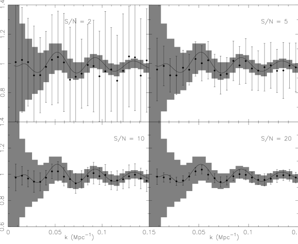
Figure 8: The data points with 1-$\sigma$ error bars display the BAO signature recovered from the 3D Ly$\alpha$ flux PS generated from a mock Ly$\alpha$ dataset containing 1200 (at $\sim 15$ per square degree) lines of sight for a $79\rm~{}deg^{2}$ survey (see text for details). Clockwise from the top left, the recovered BAO signature is extracted from spectra constructed with S/N ratios of 2, 5, 20 and 10. The error bars for varying S/N are generated using the Monte-Carlo approach described in Section 6.3.2. For comparison, the solid curve in each panel is the expected BAO signature generated from the ratio of the input linear dark matter power spectra with and without the baryon oscillation features. The shaded region, which is the same in each panel, displays an estimate of the cosmic variance error using equation (8) for our mock survey volume of $1\rm\,Gpc^{3}$.

Figure 9: Comparison of the Monte-Carlo generated shot noise errors (error bars) and the cosmic variance errors (shaded region) for varying background source density and a fixed S/N of $5$ per pixel. The Monte-Carlo shot noise errors are generated following the outline in Section 6.3.2. Clockwise from the top left, the recovered BAO signature is extracted from sight-line densities of $15$, $30$, $60$ and $45\rm~{}deg^{-2}$.

6.3 Measurement uncertainties

There are two contributions to the uncertainty on the reconstructed BAO signal we consider here; cosmic variance and shot noise. We shall estimate the former by using eight further $1\rm\,Gpc^{3}$ simulations using different random seeds to generate the initial conditions. For the latter we shall adopt a Monte-Carlo error bar estimate.

6.3.1 Cosmic variance

In Figure 7 we estimate the fractional error on the power spectrum measurement due to cosmic variance. We use nine different $1\rm\,Gpc^{3}$ simulations to generate the 3D matter (left panel) and Ly$\alpha$ forest power spectra (right panel) for each realisation. The Ly$\alpha$ power spectra from each simulation box is reconstructed using $20,000$ noiseless spectra at a density of $\sim 250\rm\,deg^{-2}$. The shot noise error due to under-sampling becomes negligible for this artificially high background source density. Using these simulations we then estimate the cosmic variance error by measuring the 1-$\sigma$ variations in the power spectra across the 9 different boxes, shown as the dashed curves in Figure 7. These are compared to the theoretical expression, displayed as the solid curves in each panel, given by equation (2) in Blake & Glazebrook (2003),

$$\left(\frac{\sigma_{P}}{P}\right)^{2}=2\frac{(2\pi)^{3}}{V}\frac{1}{4\pi k^{2}\Delta k},$$ (8)

which gives the error on a power spectrum measurement averaged over spherical $k$-bins of width $\Delta k$. For both the matter and Ly$\alpha$ forest power spectra the theoretical expression is in good agreement with our estimated cosmic variance errors except at the largest scales, $k\la 0.015$ Mpc^-1. Hence we choose to use equation (8) for cosmic variance in the remainder of this work.

6.3.2 Shot noise

We adopt a Monte-Carlo approach for estimating the shot noise on our extracted power spectrum. We randomly sample our 1 Gpc³ Ly$\alpha$ simulation (containing 100,000 lines-of-sight over $\sim 79\rm~{}deg^{2}$) and generate subsamples of 1200 spectra, yielding $\sim 15$ spectra per square degree. For each randomly generated subsample, we complete the PS reconstruction process outlined in Section 6.2. We perform this procedure 100 times using spectra which have four different signal-to-noise ratios (S/N=$2,\,5,\,10$ and $20$), and estimate the full covariance matrix and 1-$\sigma$ error for each $k$-bin.

6.3.3 Error bar estimates

In Figure 8 we compare the reconstructed BAO signature generated from our mock Ly$\alpha$ forest data to the input BAO signature generated from the matter PS for different assumptions regarding the S/N ratio of the data. The spectra have been sampled at a density of $15$ quasars per square degree (corresponding to the planned density of BOSS targets). We also compare our Monte-Carlo error bars to the expected cosmic variance error due to survey volume (shaded region) computed using equation (8).

For S/N ratios of 2 and 5 per pixel the Monte-Carlo estimates of the errors are larger than the expected cosmic variance error for a $\sim 79\rm~{}deg^{2}$ survey area. As the S/N is increased to $>10$ the recovery of the BAO signature becomes limited by cosmic variance. We reiterate that the simulations used a volume of 1 Gpc³ and that the error bars are proportional to the inverse square root of the survey area. We use a volume much smaller than a survey would require in order to illustrate the size of the error bars.

In Figure 9, we instead compare the Monte-Carlo shot noise errors to the cosmic variance error estimates while varying the background source density and assuming a fixed S/N ratio of $5$ per pixel. The line-of-sight densities are 15, 30, 45 and finally 60 quasars per square degree; background source densities larger than 45 per square degree are cosmic variance limited for our mock survey area of $79\rm~{}deg^{2}$.

6.4 Recovery of the BAO scale

We now quantify the recovery of the BAO signature from our simulations by fitting the recovered 3D Ly$\alpha$ flux PS with a function dependent on the characteristic BAO scale length. Following the approach of Blake & Glazebrook (2003), we assume a simple two parameter decaying sinusoidal model for the ratio of the 3D PS with baryonic oscillations and the smooth reference PS. The functional form of the assumed fitting function is:

$$\frac{P_{F}(k)}{P_{F,\rm{r}}(k)} = 1.0+Ak\rm{exp}\left[-\left(\frac{\it{k}}{0.1\>\it{h}\>\rm{Mpc}^{-1}}\right)^{1.4}\right]$$ (9)

$$\times\>\rm{sin}\left(\frac{2\pi\it{k}}{\it{k_{A}}}\right),$$

where $P_{F,\rm{r}}$ is the smoothed reference PS with no baryon oscillations, $A$ is an arbitrary normalisation constant and $k_{A}$ is the characteristic BAO scale in Fourier space (where the characteristic BAO scale $s_{A}=2\pi/k_{A}$). To determine the two unknown parameters we perform a $\chi^{2}$ minimisation for the ratio of the PS obtained from our simulation to the function in equation (9), such that:

$$\chi^{2}(\mn@boldsymbol{p}) = \sum_{i=1}^{n_{k}}\sum_{j=1}^{n_{k}}{\textbf{{C}}_{ij}}^{-1}[P_{\rm{ratio}}(k_{i})-P_{\rm{ratio,fit}}(\mn@boldsymbol{p},k_{i})]$$ (10)

$$\times[P_{\rm{ratio}}(k_{j})-P_{\rm{ratio,fit}}(\mn@boldsymbol{p},k_{j})],$$

where $\mn@boldsymbol{p}$ contains the parameters for the fitting formula ($A$ and $k_{A}$), and ${\textbf{{C}}_{ij}}^{-1}$ is the inverse of the covariance matrix generated from our Monte-Carlo procedure. Here $P_{\rm{ratio}}(k)$ is the ratio of the two simulated PS (with and without the baryon oscillations) and $P_{\rm{ratio,fit}}(\mn@boldsymbol{p},k)$ is given by equation (9). We restrict the range of our $\chi^{2}$ minimisation to wavenumbers below $k=0.25$ Mpc^-1, where the summation index denotes the summation over $k$ space bins in our simulated PS.

Number Density	S/N	$s_{A}$ ($2\pi/k_{A}$)	$\Delta s_{A}$	$\Delta s_{A}$ (2000 deg2)
(deg-2)		(comoving Mpc)	(per cent)	(per cent)
15	5	150.7	12.70	2.53
	10	157.4	8.51	1.70
	20	154.2	2.64	0.52
	Noiseless	153.1	0.63	0.13
45	5	155.7	5.73	1.14
	10	152.0	2.41	0.48
	20	151.9	1.23	0.24
	Noiseless	152.4	0.30	0.06

Table 1: The recovered best fitting values for the BAO scale, $s_{A}$, along with the fractional 1-$\sigma$ errors obtained by applying the $\chi^{2}$ minimisation described by equation (10) to the simulated data displayed in Figure 8. Results are shown for a background source density of $15$ and $45\rm~{}deg^{-2}$ and for S/N ratios of $5$, $10$ and $20$. The $\chi^{2}$ minimisation is performed using only the Monte-Carlo shot noise error estimates. The final row also provides the parameters recovered from noiseless data. For comparison, the input value is $s_{A}=152.5$ comoving Mpc. The final column contains the fractional error on the BAO scale after scaling our simulation result to a 2000 square degree survey area (McDonald & Eisenstein 2007).

Number Density	S/N	$s_{A}$ ($2\pi/k_{A}$ Mpc)	$\Delta s_{A}$	$\Delta s_{A}$ ($10^{4}$ deg2)
(deg-2)		(comoving Mpc)	(per cent)	(per cent)
15	5	150.7	15.51	1.38
	10	152.3	14.59	1.30
	20	152.0	6.28	0.56
	Noiseless	153.5	3.75	0.33
45	5	155.6	9.12	0.81
	10	152.6	5.66	0.50
	20	151.3	4.46	0.40
	Noiseless	151.1	4.24	0.38

Table 2: As for as Table 1, except now showing the recovered best fitting parameters for the BAO scale, $s_{A}$, using both the Monte-Carlo shot noise errors and the cosmic variance summed in quadrature. The final column contains the fractional error on the BAO scale after scaling our simulation result to a $10^{4}$ square degree survey area.

The best fit values for $s_{A}=2\pi/k_{A}$ are summarised in Table 1 for various S/N ratios (including the idealised case of noiseless data) assuming a background source density of either $15$ or $45\rm~{}deg^{-2}$. The 1-$\sigma$ relative errors on $s_{A}$ are again estimated by using 100 Monte-Carlo subsamples of mock $\mathrm{Ly}\alpha{}$ data. For each subsample we performed the $\chi^{2}$ minimisation and used the distribution of recovered values to estimate the 1-$\sigma$ relative error, $\Delta s_{A}$. The results are shown for a 1 Gpc³ volume with an area of $79\rm~{}deg^{2}$, and are also shown after scaling to $2000\rm~{}deg^{2}$ (assuming $\Delta s_{\rm A}$ is proportional to the inverse square root of the survey area). We do not quote the best fit parameters and their associated errors for S/N$=2$, as we could not recover the characteristic BAO scale at all for our small simulated volume. Even for S/N$=5$, the recovery of the BAO signal is fairly poor. However, this is to be expected for the small survey area used here, and an increase in the survey area or S/N would improve the fractional error on the recovered BAO scale considerably (McDonald & Eisenstein 2007). We nevertheless find that we are able to recover the BAO scale from our 1 Gpc³ simulations to within a few percent for S/N$>5$.

In Table 2 we again provide the best fit values for $s_{\rm A}$, but we instead perform the $\chi^{2}$ minimisation using the Monte-Carlo shot noise errors added in quadrature with the cosmic variance errors from equation (8). We find that for 15 quasars per square degree, increasing the signal to noise continues to reduce the fractional error on the BAO scale. However for 45 quasars per square degree the fractional error saturates for S/N $>$ 10, indicating the mock survey is cosmic variance limited for these parameters.

As a consistency check, we also obtain the recovered BAO signal from noiseless spectra. We performed the same 100 subsample estimation of the error bars both ignoring the estimated sample variance (Table 1) and including the sample variance (Table 2). We recover a BAO scale of 152.4 comoving Mpc (shot noise error only, 45 $\deg^{-2}$), compared with the BAO scale of the input PS which was 152.5 comoving Mpc. This confirms that our semi-analytical simulations provide a reasonable description of correlations in the density field on large scales.

We note that the two parameter fitting formula used in equation (9) does not provide a perfect description of our simulated data. There is a small reduction in the amplitude of the power spectrum toward small scales which arises following the mapping and smoothing of the initial linear density field described in Section 2. This means the oscillations do not occur exactly around one mean value as expected in the fitting formula, and this affects the recovery of the arbitrary constant, $A$, in equation (9). Importantly, however, this does not affect the recovery of the BAO scale from our simulations.

6.5 Comparison to other work

Several other authors have recently described simulations designed to recover the BAO signature from the Ly$\alpha$ forest. It is therefore constructive to compare the results presented in this work to the approaches taken by other studies using our results from Table 1. Firstly, McDonald & Eisenstein (2007) used analytical arguments to predict that one should be able measure the radial and transverse distance scales used for BAO measurements to within a fractional error of $\sim$1.4 per cent for ${\rm S/N}=1.8$ per pixel, $\sim$40 quasars per square degree and a survey area of 2000 square degrees. For a S/N of 5 per pixel over $\sim$79 square degrees for $\sim$45 quasars per square degree, we obtain a fractional error on the BAO scale of $\sim$5.7 per cent. Scaling our survey area to 2000 square degrees (assuming the error scales as the inverse square root of the survey area) we would expect a fractional error of $\sim$1.1 per cent (final column Table 1), consistent with the results of McDonald & Eisenstein (2007).

Large N-body simulations were used by Slosar et al. (2009) to measure the correlation function and also the cross-PS, rather than the 3D PS. Each dark matter N-body simulation used by Slosar et al. (2009) contained $3000^{3}$ particles in a box of size 1500 $h^{-1}$Mpc, which does not fully resolve the Jeans scale. However, the authors argue this should not affect the power on the acoustic scale. They conclude that the correlation function provides a better method for recovery of the BAO signal compared to both the 3D flux PS and the cross-PS, which is consistent with the approach taken by White et al. (2010). Slosar et al. (2009) fit for the BAO peak at $z=2.5$ using $\sim$56 quasars per square degree over a total area of $\sim 400$ square degrees. For noiseless spectra we find a fractional error on the BAO scale of 0.30 per cent compared to 0.53 per cent from Slosar et al. (2009). The survey area of Slosar et al. (2009) is $\sim$5 times larger than ours, implying an error that should be $\sim$2.2 times smaller than our error. The origin of this difference is unclear, but may be in part due to the use of the diagonal covariance by Slosar et al. (2009), as opposed to the full covariance matrix we use in our best-fit parameter estimation.

Finally, we compare our results to those of McQuinn & White (2011) who provide sensitivity estimates for large Ly$\alpha$ forest surveys. Although a direct comparison here is less straightforward, using their table 4, a background source density of $\sim 15\rm~{}deg^{-2}$ corresponds to an $\bar{n}_{eff}=1.4\times 10^{-3}$ Mpc^-2 at $z=2.5$. However, at $z=2.5$ for S/N = 2, the effective number density varies from the true number density by roughly 0.59 (their table 3) and so $\bar{n}_{eff}\sim 0.8\times 10^{-3}$ Mpc^-2. From figure 8 in McQuinn & White (2011), this gives the fractional precision in the angular diameter distance and Hubble expansion of $\sim 2-3$ per cent for a $\sim 10^{4}$ square degree survey volume at $z=2.5$. Scaling our $z=3$ results for the fractional precision of the BAO scale assuming S/N of 2 (Section 7), a survey area of $10^{4}\rm\,deg^{2}$ and 15 quasars per square degree, we find a fractional precision of $\sim 2.5$ per cent on the BAO scale. McQuinn & White (2011) also find that the amount of information obtained from a quasar is maximised for S/N $\sim$5-10, consistent with our findings in Figure 8.

7 Approximate scaling relations for the fractional error

To summarise our results we provide approximate scaling relations for the expected recovered fractional error on the BAO scale as a function of both survey S/N and quasar number density. We approximate this using a simple power law expression,

$$\rm{fractional~{}error~{}(per~{}cent)}=ax^{b}\left(\frac{\textrm{Survey area}}{79~{}\textrm{deg${}^{2}$}}\right)^{-1/2},$$ (11)

where x is either S/N (Table 3) or quasar number density (Table 4) and perform a least squares fit on our simulation results. We provide the best fit parameters $a$ and $b$ for the fractional error fit for the shot noise errors alone, as well as the shot noise added in quadrature with the cosmic variance. The fractional error also scales as the inverse square root of the survey area.

7.1 Scaling constraints to a BOSS-like survey

Using the best fit parameters from our model for the BAO scale from Table 2, we can estimate the accuracy of forthcoming large volume BAO Ly$\alpha$ forest surveys. BOSS anticipates the detection of 150,000 quasars in a total survey area of $10^{4}\rm~{}deg^{2}$, with S/N = 5 and a source number density of $15\rm~{}deg^{-2}$. Scaling our simulation results from Table 2, we anticipate a detection of the BAO scale to within $\sim$1.4 per cent including cosmic variance.

Error	Number Density	$a$	$b$
	(sq. deg.)
Shot noise	15	52.85	-0.91
	45	26.50	-1.04
Shot noise	15	41.34	-0.54
$+$cosmic variance	45	27.55	-0.66

Table 3: Best fit parameters for $a$ and $b$ in equation (11) for the fractional error on $s_{A}$ for varying S/N (the models used to obtain the scaling fit have S/N=2, 3.5, 5, 7.5, 10, 15 and 20). Scalings are given for background source densities of both 15 and 45 quasars per square degree, and a total survey area of $79\rm~{}deg^{2}$. Top row: Fit parameters for Monte-Carlo shot noise error bars only. Bottom row: Fit parameters for shot noise and cosmic variance errors added in quadrature.

Error	S/N	$a$	$b$
Shot noise	5	99.12	-0.78
	10	140.39	-1.14
Shot noise	5	76.16	-0.61
$+$cosmic variance	10	53.35	-0.55

Table 4: Best fit parameters for $a$ and $b$ in equation (11) for the fractional error on $s_{A}$ for varying quasar sightline density (the models used to obtain the scaling fit have 5, 10, 15, 22.5, 30, 45 and 60 $\rm deg^{-2}$). Scalings are given for both S/N = 5 and 10, and a total survey area of $79\rm~{}deg^{2}$. Top row: Fit parameters for Monte-Carlo shot noise error bars only. Bottom row: Fit parameters for shot noise and cosmic variance errors added in quadrature.

8 Conclusion

A series of recent studies have used large volume, high resolution N-body and hydrodynamical simulations to study the detection of BAO in forthcoming large volume Ly$\alpha$ forest surveys (such as BOSS). One limitation of these simulations is the large computational cost required for a simulation of sufficient volume. On the other hand, in order to study the systematics involved in the detection of the BAO signal, it will be critical to run many simulations to fully probe parameter space. In this work we have demonstrated that a semi-analytical model utilising a density field calibrated against a hydrodynamical simulation can be used to produce very large volume, high resolution simulations at a fraction of time and computational cost, and at a reasonable level of accuracy. We find good quantitative agreement between the semi-analytical model and the hydrodynamical simulation for a range of observables. In particular, we are able to reproduce one and two-point statistics (the flux PDF and PS), which are in reasonable agreement with observational data. We stress that in this work we assume a constant redshift, $z=3$, whereas one expects that the accuracy of the recovered BAO scale with be redshift dependant, and hence our results will differ slightly for different redshifts.

We used our model to generate mock Ly$\alpha$ forest data sets drawn from a 4096³ 1 Gpc³ simulation volume. We demonstrated we are able to recover the BAO signal through reconstruction of the 3D Ly$\alpha$ PS (McDonald & Eisenstein, 2007). We also recover the characteristic BAO scale length by applying a $\chi^{2}$ minimisation with a simple two parameter fitting function (Blake & Glazebrook, 2003). We used Monte-Carlo realisations of the Ly$\alpha$ forest data to estimate the $1-\sigma$ uncertainties on the PS due to shot noise for varying S/N and background source densities, and include an estimate of cosmic variance error from our nine 1 Gpc³ simulations. Our mock surveys of $\sim$ 15 quasars per square degree over $\sim$ 79 square degrees with S/N = (5, 10, 20, $\infty$) yield relative errors of (12.7, 8.51, 2.64, 0.63) per cent and for $\sim$ 45 quasars per square degree (5.73, 2.41, 1.23, 0.30) per cent on the recovered BAO scale. The accuracy to which we can recover the BAO scale with square root of the inverse volume, and are consistent with the predictions presented by McDonald & Eisenstein (2007), Slosar et al. (2009) and McQuinn & White (2011).

Using the results of our mock Ly$\alpha$ analysis, we anticipate that for a S/N = 5 with 15 quasars per square degree for a BOSS-like survey of $10^{4}\rm~{}deg^{2}$, one should expect a fractional error of $\sim$ 1.4 per cent on the BAO scale. We also provide simple scaling relations for estimating the expected fractional error on the BAO scale given the number density of quasars and the signal to noise.

The method presented here enables generation of large scale realisations of the IGM density field and Ly$\alpha$ forest quickly and efficiently. It is therefore ideal for investigating the key systematics which will impact on BAO detection, such as errors in the continuum shape and the effect of non-gravitational fluctuations on the Ly$\alpha$ forest, including large-scale temperature and ionisation variations in the IGM at $z=3$.

Appendix A GPGPU

In this appendix we describe the use of GPGPU (General Purpose computing on Graphics Processing Units) programming in our simulations. Our code has been implemented in three formats, single core, parallelised multicore and a mix of parallel multicore and GPU programming. The larger simulations used in this paper are performed using both a parallel multicore and a single GPU. For all simulations we use an Intel Xeon 2.00Ghz quad core CPU and a nVidia FX580 CUDA enabled graphics card.

Over the last few years major steps have been taken in the implementation of GPU programming into many astrophysical applications. Implementations of current astrophysical simulations with GPUs can report upward of a 10-100 factor speed up in computational time (see Fluke et al., 2010, and references therein). One of the major problems for GPU programmers is how to take full advantage of a GPU for solving computational problems. One must maximise usage of on-chip resources, while allowing as much of the calculation to be run without intervention from the host CPU. One must also avoid data dependency, where a result at one point in the data can impact on the outcome of a separate piece of data (i.e. data must be as independent as possible). The transfer of data from the CPU and GPU can also limit the effectiveness of the GPU programming application, and is dependent on the details of the individual’s computer.

The goal of our simulations is to provide a model that can be used to investigate the $\mathrm{Ly}\alpha$ forest. To accomplish this we only generate a limited number of sightlines per simulation rather than the entire density field (i.e. we generate our density field in Fourier space, and only Fourier transform the number of sightlines required). Our semi-analytical model is perfectly suited for implementation on a GPU, allowing us to quickly run mock survey simulations in less than a day.

In Figures 10 and 11, we show the increase in performance gained by using a GPU for certain functions in our simulation, relative to single and parallelised quad core implementations. Figures 10 and 11 show the total runtime of the individual section of the code used to generate the Fourier space density field and for calculating the spherically averaged 3D PS. We scale up the number of pixels along the length of the simulation cube in powers of two, from 256 to 4096. We include in the timing all required overhead, such as data transfer from CPU to GPU and memory allocation.

For calculation of the Fourier space density field we observe a reduction in runtime by roughly a factor of 4 on moving from the single to quad core implementation, with a further factor of 4 from quad core to GPU. For the 3D PS, we observe a factor 3 decrease in runtime from single to quad core, and a factor of 8 decrease from quad to GPU. Although our the decrease in runtime is only a factor of $\sim$4-8 (relative to the parallelised CPU) for our two chosen processes, this is mainly due to the specific GPU used. Our GPU contains only 1.12Ghz clock speed, with a maximum of 32 cores, whereas top of the line GPGPUs allow up to as many as 440 cores with clock speeds of 1.3Ghz. Implementation of our GPU enabled code onto one of the newest devices would facilitate the 10-100 factor increase in computational speed.

A considerable amount of computational time is taken up by Fourier transformation of our simulated data. Although not implemented in the current version of our code, initial testing of the inbuilt FFT libraries provided show an expected additional factor of $\sim$10 reduction in computation time, which would further reduce our total computation time.

Figure 10: Computation time for the generation of the density field in Fourier space as a function of the pixel number per side of a simulation cube. The solid curve shows the timings for a single core calculation, the dashed for quad core, and the dot-dashed curve is obtained using the GPU. The timing takes into account all required overhead such as data transfer between devices and memory allocation.

Figure 11: Computation time for the generation of the 3D PS as a function of the pixel number per side of a simulation cube. The curves are as described for Figure 10.

Appendix B Memory limitations when generating large simulation boxes

In this work we have used our code to generate 4096³ simulation boxes on a desktop PC. However on a desktop PC we are memory limited and cannot store the entire box in memory at once. We circumvent this problem by using the natural symmetry of the density field in Fourier space to break up our large simulation volume into 8 smaller simulation volumes. However, even these 8 smaller simulation volumes cannot be fully read into memory at one time, and hence we only read into memory a small section of the volume at any one time. The advantage of such an approach is that our code can be performed easily on any desktop computer.

Instead of computing the 3D FFTs (Fast Fourier Transform) which would require the full simulation to be read into memory, we again use the symmetry of the density field and Fourier transform in 2D slices across our large simulation volume (reading in the necessary 4 smaller simulation volumes for each 2D slice). We then only Fourier transform out the final 1D lines of sight that we have randomly generated throughout the full simulation volume. This final step of only Fourier transforming the final 1D line of sight is well suited for generating mock Ly$\alpha$ forest surveys.

References

- Becker et al. (2011) Becker G. D., Bolton J. S., Haehnelt M. G., Sargent W. L. W., 2011, Monthly Notices of the Royal Astronomical Society, 410, 1096
- Beutler et al. (2011) Beutler F., et al., 2011, eprint arXiv, 1106, 3366, 18 pages, 17 figures, 3 tables
- Bi (1993) Bi H., 1993, Astrophysical Journal, 405, 479
- Bi & Davidsen (1997) Bi H., Davidsen A. F., 1997, Astrophysical Journal v.479, 479, 523
- Blake et al. (2007) Blake C., Collister A., Bridle S., Lahav O., 2007, Monthly Notices of the Royal Astronomical Society, 374, 1527
- Blake & Glazebrook (2003) Blake C., Glazebrook K., 2003, The Astrophysical Journal, 594, 665
- Blake et al. (2011) Blake C., et al., 2011, Monthly Notices of the Royal Astronomical Society, 951
- Bolton & Becker (2009) Bolton J. S., Becker G. D., 2009, Monthly Notices of the Royal Astronomical Society: Letters, 398, L26
- Bolton et al. (2010) Bolton J. S., Becker G. D., Wyithe J. S. B., Haehnelt M. G., Sargent W. L. W., 2010, Monthly Notices of the Royal Astronomical Society, 406, 612, (c) Journal compilation © 2010 RAS
- Bolton et al. (2009) Bolton J. S., Oh S. P., Furlanetto S. R., 2009, Monthly Notices of the Royal Astronomical Society, 395, 736
- Bolton et al. (2008) Bolton J. S., Viel M., Kim T.-S., Haehnelt M. G., Carswell R. F., 2008, Monthly Notices of the Royal Astronomical Society, 386, 1131
- Cen et al. (1994) Cen R., Miralda-Escudé J., Ostriker J. P., Rauch M., 1994, Astrophysical Journal, 437, L9
- Choudhury et al. (2001) Choudhury T. R., Srianand R., Padmanabhan T., 2001, The Astrophysical Journal, 559, 29
- Cole et al. (2005) Cole S., et al., 2005, Monthly Notices of the Royal Astronomical Society, 362, 505
- Coles & Jones (1991) Coles P., Jones B., 1991, Royal Astronomical Society, 248, 1
- Croft et al. (2002) Croft R. A. C., Weinberg D. H., Bolte M., Burles S., Hernquist L., Katz N., Kirkman D., Tytler D., 2002, The Astrophysical Journal, 581, 20
- Desjacques & Nusser (2005) Desjacques V., Nusser A., 2005, Monthly Notices of the Royal Astronomical Society, 361, 1257
- Desjacques et al. (2007) Desjacques V., Nusser A., Sheth R. K., 2007, Monthly Notices of the Royal Astronomical Society, 374, 206
- Eisenstein & Hu (1998) Eisenstein D. J., Hu W., 1998, Astrophysical Journal v.496, 496, 605, (c) 1998: The American Astronomical Society
- Eisenstein et al. (2005) Eisenstein D. J., et al., 2005, The Astrophysical Journal, 633, 560
- Eisenstein et al. (2011) —, 2011, eprint arXiv, 1101, 1529, submitted to the Astronomical Journal
- Fluke et al. (2010) Fluke C. J., Barnes D. G., Barsdell B. R., Hassan A. H., 2010, arXiv, astro-ph.IM
- Gnedin & Hui (1996) Gnedin N. Y., Hui L., 1996, Astrophysical Journal Letters v.472, 472, L73, (c) 1996: The American Astronomical Society
- Gnedin & Hui (1998) —, 1998, Monthly Notices of the Royal Astronomical Society, 296, 44
- Hernquist et al. (1996) Hernquist L., Katz N., Weinberg D. H., Miralda-Escudé J., 1996, Astrophysical Journal Letters v.457, 457, L51
- Hui et al. (1997) Hui L., Gnedin N. Y., Zhang Y., 1997, Astrophysical Journal v.486, 486, 599
- Hütsi (2006) Hütsi G., 2006, Astronomy and Astrophysics, 449, 891
- Kim et al. (2007) Kim T.-S., Bolton J. S., Viel M., Haehnelt M. G., Carswell R. F., 2007, Monthly Notices of the Royal Astronomical Society, 382, 1657
- Kim et al. (2004) Kim T.-S., Viel M., Haehnelt M. G., Carswell R. F., Cristiani S., 2004, Monthly Notices of the Royal Astronomical Society, 347, 355
- Kitaura et al. (2010) Kitaura F.-S., Gallerani S., Ferrara A., 2010, arXiv, astro-ph.CO
- Lidz et al. (2010) Lidz A., Faucher-Giguère C.-A., Dall’Aglio A., McQuinn M., Fechner C., Zaldarriaga M., Hernquist L., Dutta S., 2010, The Astrophysical Journal, 718, 199
- Matarrese & Mohayaee (2002) Matarrese S., Mohayaee R., 2002, Monthly Notices of the Royal Astronomical Society, 329, 37
- McDonald & Eisenstein (2007) McDonald P., Eisenstein D. J., 2007, Physical Review D, 76, 63009
- McDonald et al. (2000) McDonald P., Miralda-Escudé J., Rauch M., Sargent W. L. W., Barlow T. A., Cen R., Ostriker J. P., 2000, The Astrophysical Journal, 543, 1
- McDonald et al. (2005) McDonald P., et al., 2005, The Astrophysical Journal, 635, 761, (c) 2005: The American Astronomical Society
- McQuinn et al. (2009) McQuinn M., Lidz A., Zaldarriaga M., Hernquist L., Hopkins P. F., Dutta S., Faucher-Giguère C.-A., 2009, The Astrophysical Journal, 694, 842
- McQuinn & White (2011) McQuinn M., White M., 2011, Monthly Notices of the Royal Astronomical Society, 727
- Meiksin (2009) Meiksin A. A., 2009, Reviews of Modern Physics, 81, 1405
- Norman et al. (2009) Norman M. L., Paschos P., Harkness R., 2009, Journal of Physics: Conference Series, 180, 2021
- Padmanabhan et al. (2007) Padmanabhan N., et al., 2007, Monthly Notices of the Royal Astronomical Society, 378, 852
- Percival et al. (2007) Percival W. J., Cole S., Eisenstein D. J., Nichol R. C., Peacock J. A., Pope A. C., Szalay A. S., 2007, Monthly Notices of the Royal Astronomical Society, 381, 1053
- Percival et al. (2010) Percival W. J., et al., 2010, Monthly Notices of the Royal Astronomical Society, 401, 2148
- Rauch (1998) Rauch M., 1998, Annual Review of Astronomy and Astrophysics, 36, 267
- Reisenegger & Miralda-Escude (1995) Reisenegger A., Miralda-Escude J., 1995, Astrophysical Journal v.449, 449, 476
- Richards et al. (2006) Richards G. T., et al., 2006, The Astronomical Journal, 131, 2766
- Schaye et al. (2000) Schaye J., Theuns T., Rauch M., Efstathiou G., Sargent W. L. W., 2000, Monthly Notices of the Royal Astronomical Society, 318, 817
- Schlegel et al. (2009) Schlegel D., White M., Eisenstein D., 2009, Astro2010: The Astronomy and Astrophysics Decadal Survey, 2010, 314
- Seo & Eisenstein (2007) Seo H.-J., Eisenstein D. J., 2007, The Astrophysical Journal, 665, 14
- Slosar et al. (2009) Slosar A., Ho S., White M., Louis T., 2009, Journal of Cosmology and Astroparticle Physics, 10, 019
- Slosar et al. (2011) Slosar A., et al., 2011, arXiv, astro-ph.CO
- Springel (2005) Springel V., 2005, Monthly Notices of the Royal Astronomical Society, 364, 1105
- Theuns et al. (1998) Theuns T., Leonard A., Efstathiou G., Pearce F. R., Thomas P. A., 1998, Monthly Notices of the Royal Astronomical Society, 301, 478
- Valageas et al. (2002) Valageas P., Schaeffer R., Silk J., 2002, Astronomy and Astrophysics, 388, 741
- Viel et al. (2009) Viel M., Bolton J. S., Haehnelt M. G., 2009, Monthly Notices of the Royal Astronomical Society: Letters, 399, L39
- Viel et al. (2004) Viel M., Haehnelt M. G., Springel V., 2004, Monthly Notices of the Royal Astronomical Society, 354, 684
- Viel et al. (2002a) Viel M., Matarrese S., Mo H. J., Haehnelt M. G., Theuns T., 2002a, Monthly Notices of the Royal Astronomical Society, 329, 848
- Viel et al. (2002b) Viel M., Matarrese S., Mo H. J., Theuns T., Haehnelt M. G., 2002b, MNRAS, 336, 685
- White et al. (2010) White M., Pope A., Carlson J., Heitmann K., Habib S., Fasel P., Daniel D., Lukic Z., 2010, The Astrophysical Journal, 713, 383
- Zel’Dovich (1970) Zel’Dovich Y. B., 1970, Astron. Astrophys., 5, 84, a&AA ID. AAA003.061.016
- Zhan et al. (2005) Zhan H., Knox L., Tyson J. A., Margoniner V., 2005, in Bulletin of the American Astronomical Society, Vol. 37, American Astronomical Society Meeting Abstracts, pp. 1202–+