Model of bound interface dynamics for coupled magnetic domain walls

Abstract

A domain wall in a ferromagnetic system will move under the action of an external magnetic field. Ultrathin Co layers sandwiched between Pt have been shown to be a suitable experimental realization of a weakly disordered 2D medium in which to study the dynamics of 1D interfaces (magnetic domain walls). The behavior of these systems is encapsulated in the velocity-field response $v(H)$ of the domain walls. In a recent paper [P.J. Metaxas et al., Phys. Rev. Lett. 104, 237206 (2010)] we studied the effect of ferromagnetic coupling between two such ultrathin layers, each exhibiting different $v(H)$ characteristics. The main result was the existence of bound states over finite-width field ranges, wherein walls in the two layers moved together at the same speed. Here, we discuss in detail the theory of domain wall dynamics in coupled systems. In particular, we show that a bound creep state is expected for vanishing $H$ and we give the analytical, parameter free expression for its velocity which agrees well with experimental results.

I Introduction

A number of physical phenomena involve elastic interfaces moving through disordered media. These phenomena range from domain wall motion in ferromagnets Lemerle et al. (1998); Repain et al. (2004); Metaxas et al. (2007); Kim et al. (2009), ferroelectrics Paruch et al. (2006) and multiferroics Catalan et al. (2008) to wetting Balankin et al. (2000) as well as vortex motion in high-T${}_{\hbox{\tiny C}}$ superconductors Blatter et al. (1994). The theoretical frameworks Blatter et al. (1994); Chauve et al. (2000); Kolton et al. (2009) developed to model elastic interface dynamics are therefore highly relevant for a number of real world processes which are of interest both for their fundamental properties and eventual applications. Indeed, theoretical studies of single interface dynamics and statics have revealed a lot of interesting physics with predictions of universality, in-depth studies of dynamic and static critical exponents Huse and Henley (1985); Huse et al. (1985); Kardar (1985); Chauve et al. (2000); Kolton et al. (2009) and the development of now well-known interface growth equations Barabasi and Stanley (1995). Magnetic systems in particular have been an ideal testing ground for these theories Lemerle et al. (1998); Krusin-Elbaum et al. (2001); Repain et al. (2004); Metaxas et al. (2007); Kim et al. (2009) since these systems can be easily probed and manipulated.

A relatively recent theoretical, and more recently, experimental, playground has been developing concerning the physics of interacting interfaces in 2D systems. Theoretically, this problem has been studied via modified growth equations Barabási (1992); Majumdar and Das (2005), Monte Carlo modeling of repulsive or non-interacting interfaces Juntunen et al. (2007); Juntunen and Merikoski (2010) and scaling arguments Bauer et al. (2005). Quasi-2D experimental realizations of systems containing coupled interfaces have also been conceived, ranging from interacting fluid fronts Balankin et al. (2006) to repulsive Bauer et al. (2005) and attractive Metaxas et al. (2010); SanEmeterioAlvarez2010 magnetic domain walls.

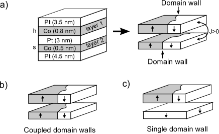
Figure 1: (a) Using magnetic layers coupled via an interlayer interaction energy, $J$, to create a model system for studying bound domain walls. Measurements of domain wall motion in this system consisted either of (b) coupled domain walls (boundaries of domains which are statically aligned in zero field) or (c) single domain walls (boundaries of domains existing in the hard layer only).

Our work on field-driven, attractively coupled domain walls Metaxas et al. (2010) has been carried out on a system consisting of two physically separate, but magnetically coupledMoritz et al. (2004), ultrathin ferromagnetic Co layers [Fig. 1(a)]. The ferromagnetic coupling tends to align the magnetization in the two layers. Therefore, if a domain wall is present in each Co layer [eg. Fig. 1(b)], the ferromagnetic coupling will tend to align them, acting as an attractive interaction between the walls. This attraction not only favors a static domain wall alignment in zero-field, but can also stabilize the aligned state dynamically under an applied fieldMetaxas et al. (2010). In this case, walls in the two layers are dynamically bound and move together at a common, unique velocity, despite each wall having different intrinsic velocity-field responses. These differing velocity-field responses however do mean that dynamic domain wall binding can occur only over field ranges in which wall velocities in each layer are sufficiently close, placing a limit on the fields for which bound motion can occur. Until this work, studies of pairs of interacting interfaces in quasi-2D systems had been mostly carried out in single media. While it was already thought that domain walls in strongly coupled layers moved together Wiebel et al. (2005, 2006); Metaxas et al. (2009), this was the first study wherein both dynamically bound domain walls and transitions between bound and unbound dynamics were directly evidenced.

In this article, we discuss in detail a theoretical description of bound domain wall motion. The paper is outlined as follows. In Sec II we briefly give some details about the model system. In Sec. III we analyze how domain wall speed is affected by interlayer coupling and in Sec. IV we study analytically the bound state regimes and discuss the agreement between theory and experiment. A short conclusion follows.

II Coupled ultrathin magnetic layers

The experimental system shown in Fig. 1(a) is a magnetic multilayer consisting of two ultrathin Co layers: a magnetically hard 0.8 nm layer (layer 1) and a softer 0.5 nm layer (layer 2). The layers are ferromagnetically coupled Moritz et al. (2004) (coupling energy $J>0$) across a 3 nm thick Pt spacer. Seed and capping Pt layers ensure an out-of-plane magnetic anisotropy within the Co layers. Pt/Co-based films are now considered good experimental realizations of a weakly disordered, ferromagnetic 2D Ising system, due to their anisotropy-induced out-of-plane magnetization, narrow domain walls and intrinsic structural disorder Lemerle et al. (1998); Metaxas et al. (2007). This disorder has a major role in determining the velocity response $v(H)$ of a domain wall to an external field $H$, applied perpendicular to the film plane.

Two types of domain wall velocity measurements were carried out based upon the two domain (wall) types which could be nucleated within the multilayer. Both types of wall could be propagated under field to determine their velocity-field responses using a quasi-static magneto-optical method Metaxas et al. (2007, 2010). (1) Coupled domain walls are the boundaries of domains existing in both layers which, in zero field, are aligned spatially with their magnetizations pointing in the same direction, as shown in Fig. 1(b). Under field, and depending on the field amplitude, they can move together, in a dynamically bound state, or separately. (2) Single domain walls are the boundaries of domains existing in the hard layer only, as illustrated in Fig. 1(c). Measurements of these domain walls yield a reference velocity and a determination of the interlayer coupling.

III From isolated to coupled and bound domain wall dynamics

Here we analyze field-velocity responses of: i) a single domain wall in an isolated magnetic layer, ii) a single domain wall in one magnetic layer coupled to a second, saturated magnetic layer, and iii) two coupled domain walls, one in the hard layer and the other in the soft layer. Domain walls will be approximated as straight lines, whose position is given by a single number. We begin with a single wall located at $x=x_{w}$ in an isolated ultrathin Co layer [see Fig. 2(a)]. The Co layer is positively magnetized for $x<x_{w}$ and negatively magnetized for $x>x_{w}$. The application of an external field $H>0$ drives the wall to the right, with the wall acquiring a positive velocity $v(H)=dx_{w}/dt$. Experimental resultsMetaxas et al. (2007) obtained for domain wall motion in Pt/Co(0.5-0.8 nm)/Pt films show that $v(H)$ is characterized by two distinct regimes at room temperature (creep and flow) which were theoretically predictedBlatter et al. (1994); Chauve et al. (2000) and are sketched in the schematic of Fig. 2(b). Domain walls exhibit flow motion at high fields for which $v\propto H$. However, below a layer-dependent critical depinning field $H_{\hbox{\tiny dep}}$ (generally on the order of a few hundred OerstedMetaxas et al. (2007)), disorder-induced pinning effects become significant and the walls exhibit thermally activated creepLemerle et al. (1998). Within this latter regime, $v(H)$ has the form

$$v(H)=v_{0}\exp\left[-{U_{C}\over k_{B}T}\left({H_{\hbox{\tiny dep}}\over H}\right)^{1/4}\right],$$ (1)

where the exponential factor $U_{C}/k_{B}T$ is the ratio between the typical pinning energy and the thermal energy. The exponent $1/4$ is a universal exponent, characteristic of the dynamics of a one dimensional interface in a 2D weakly disordered medium.

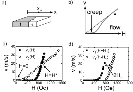
Figure 2: (a) The average domain wall position is denoted $x_{w}$. (b) At finite temperature, walls exhibit a low field, thermally activated creep regime and a high field, dissipation-limited, linear flow regime. The two are separated by a thermally smeared depinning transitionBustingorry et al. (2008) (not labeled). (c) Experimentally obtained domain wall dynamics in layers 1 and 2 in the absence of coupling. The two curves cross at $H=0$ and $H=H^{*}$. (d) Domain wall dynamics in layer 1 for a coupling field, $H_{1}$, which reinforces the applied field $H$, ($v_{1}(H+H_{1})$) or works against it ($v_{1}(H-H_{1})$).

Films with different thicknesses have different microscopic parameters and disorder strengths. As a result, they have different $v(H)$ characteristicsMetaxas et al. (2007), as attested by the experimental velocity-field curves for domain walls in the two layers in the absence of coupling [Fig. 2(c)]. However, pairs of such curves often intersect at two points: $H=0$ and $H=H^{*}$ ($H^{*}\simeq 860$ Oe for our system). The first crossing point is universal, because the velocity $v(f)$ of any isolated interface in response to a generalized force $f$ (here, $f=H$) is always expected to vanish for vanishing $f$. The second crossing point is less trivial and arises because domain walls in thicker Co layers generally have a lower creep velocity but a higher flow velocity than walls in thinner layers.

In the remainder of this article, we shall use $v_{1}(H)$ to refer to the domain wall velocity in the hard layer and $v_{2}(H)$ to that in the soft layer. If the two films are not coupled, it is clear that walls will propagate independently, with $v_{2}>v_{1}$ for $H<H^{*}$ and $v_{1}>v_{2}$ for $H>H^{*}$ [Fig. 2(c)]. The question we are now going to consider is the following: What is the effect of interlayer coupling on domain wall velocities $v_{1,2}(H)$ and domain wall binding phenomena?

Before considering coupling between domain walls, let us consider the simpler case of a single domain wall in layer $i=1,2$, interacting with a uniformly magnetized layer $k=2,1$ (see, for example, Fig. 1(c)). The interlayer coupling $J$ induces an effective coupling field $h_{i}$, given by Grolier et al. (1993)

$$h_{i}=m_{k}\frac{J}{M_{\hbox{\tiny S}}^{i}t_{i}}\equiv m_{k}H_{i},$$ (2)

where $M_{\hbox{\tiny S}}$ is the saturation magnetization, $t$ is the layer thickness, and $m=\pm 1$ is the magnetization orientation. $h_{i}$ adds to the external field $H$ and also drives the domain wallFukumoto2005 ; Metaxas et al. (2008), in turn allowing for a simple experimental determination of $H_{i}$. To determine $H_{1}$, domain wall velocities in the hard layer were measured while keeping the soft layer magnetically saturated. Through control of $m_{2}$ and/or $H$, it was possible to determine wall velocities with $h_{1}$ either opposing or reinforcing the applied field. We denote these data sets $v_{1}(H-H_{1})$ and $v_{1}(H+H_{1})$ respectively. Plotted in Fig. 2(d), the two data sets are separated by $2H_{1}$, allowing a determination of $H_{1}=120$ Oe and $v_{1}(H)$ [ie. no coupling, see Fig. 2(c)].

The corresponding coupling field and isolated wall dynamics for layer 2 were determined in a different manner. $H_{2}=220$ Oe could be easily found using Eq. (2), which gives $H_{1}M_{\hbox{\tiny S}}^{1}t_{1}=H_{2}M_{\hbox{\tiny S}}^{2}t_{2}$ ($M_{\hbox{\tiny S}}^{1,2}$ are known Metaxas et al. (2010)). Unfortunately, we were not able to nucleate a domain in the soft layer while keeping the hard layer in a single domain state and so $v_{2}(H)$ had to be measured using a Co(0.5 nm) layer in a less strongly coupled Pt/Co(0.5 nm)/Pt(4 nm)/Co(0.8 nm)/Pt film Metaxas et al. (2008).

Now, let’s turn to dynamics of coupled walls [Fig. 1(b)]. The experimental determination of the coupled walls is as follows. (i) Two aligned domain walls, at a common position $x_{1}(0)=x_{2}(0)$, are nucleated. (ii) A magnetic field pulse, $H$, is applied for a time $T$, under which walls move to positions $x_{1}(T),x_{2}(T)$. (iii) The new wall positions are quasi-statically determinedMetaxas et al. (2007, 2010) from Kerr microscopy images.

While $x_{1}(T)=x_{2}(T)$ for dynamically bound walls, $x_{1}(T)\neq x_{2}(T)$ for unbound walls since the walls separate during their motion. However, the time interval between steps (ii) and (iii) is large enough to allow the separated walls to relax back to an aligned state under the action of effective coupling fields ($H=0$ for $t>T$). Since $v_{2}(H_{2})/v_{1}(H_{1})\approx 10^{10}$, if $x_{1}(T)\neq x_{2}(T)$, pre-imaging relaxation of the soft layer wall gives: $x_{2}^{\hbox{\tiny imaged}}=x_{1}(T)$. Therefore, the experimental technique yields either the true bound wall displacement (and subsequently the bound velocity) or the hard wall displacement (and therefore the hard layer wall velocity) when the walls are unbound.

In the unbound state, the hard layer velocity (and therefore the experimentally determined velocity of the coupled walls), will be that observed for hard layer walls under a field $H\pm H_{1}$ [Fig. 2(d)] since the walls in the two layers are not aligned: $+H_{1}$ if the hard layer wall trails the soft layer wall and $-H_{1}$ if the hard layer wall leads the soft layer wall [Eq. (2)]. This is an important point, as it allows us to identify the field ranges over which $v_{\hbox{\tiny C}}(H)$ (the experimentally obtained coupled wall velocity) corresponds to unbound motion. The unbound (U) and bound (B) regions are labeled in Fig. 3(a) in which $v_{\hbox{\tiny C}}(H)$ is plotted together with $v_{1}(H\pm H_{1})$ to allow a direct comparison. This allows us to easily locate the three critical fields, $H_{c1,2,3}$, which separate bound and unbound states [see vertical lines in Figs. 3(a,b)]: $H_{c1}\approx 250$Oe, $H_{c2}\approx 750$Oe, and $H_{c3}\approx 1150$Oe.

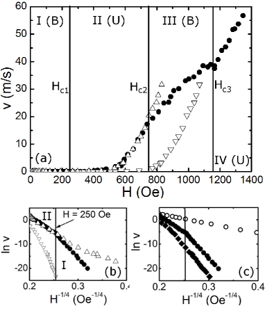
Figure 3: (a and b) Experimentally obtained coupled wall velocity, $v_{\hbox{\tiny C}}(H)$ ($\bullet$) plotted with hard domain velocities in the presence of a positively saturated soft layer, $v_{1}(H+H_{1})$ ($\bigtriangleup$) and a negatively saturated soft layer, $v_{1}(H-H_{1})$ ($\bigtriangledown$). Field regions in which bound (B) and unbound (U) coupled wall dynamics are labeled with roman numerals. Vertical solid lines represent the region limits ($H_{c(1,2,3)}$). (c) $v_{\hbox{\tiny C}}(H)$ ($\bullet$) compared to hard and soft layer domain wall creep velocities in the absence of coupling, $v_{1}(H)$ ($\blacklozenge$) and $v_{2}(H)$ ($\circ$) respectively.

We first consider the unbound field ranges. In region II, $H_{c1}<H<H_{c2}$ of Fig. 3(a), $v_{2}(H)\gg v_{1}(H)$ [see Fig. 2(c)], so that the soft domain wall leads and the distance $(x_{2}-x_{1})$ between walls is positive and large. The soft wall is so far ahead of the hard wall that the latter moves under the action of a positively saturated soft layer. When $H>H_{c3}$, the situation is reversed: $v_{1}(H)\gg v_{2}(H)$ [see Fig. 2(c) again]. The hard domain wall leads and the soft wall is so far behind it that the hard wall moves under the action of a negatively saturated soft layer. A schematic of these regimes is shown in Fig. 4.

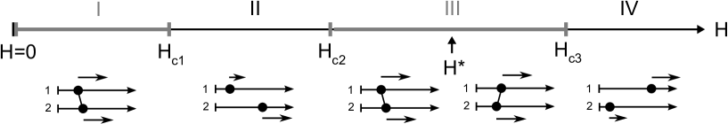
Figure 4: This figure shows the different field regimes. In the unbound states (thin, black lines), walls in layer 1 and 2 move at different speeds, the leading wall at a higher velocity. In the bound states (thick, grey lines), walls move at the same speed. The distance between walls is therefore constant. The leading wall is the wall with the higher velocity, in the absence of coupling.

While we can compare $v_{\hbox{\tiny C}}(H)$ to $v_{1}(H\pm H_{1})$ to obtain values for the region limits $H_{cj}$ ($j=1,2,3$), these values can also be evaluated from the experimentally obtained velocity data in Fig. 2(c) and the $H_{1,2}$ values. Before moving on to analytical and numerical modeling results, we explain how this is done using a simple graphical method.

In regime II, the walls in each layer move separately with the soft wall leading. This can be sustained only if

$$v_{2}(H-H_{2})>v_{1}(H+H_{1}).$$ (3)

Therefore, it is straightforward to define the critical fields $H_{c1}$ and $H_{c2}$ through the equation

$$v_{2}(H-H_{2})=v_{1}(H+H_{1}).$$ (4)

This equation can be solved graphically using the data in Fig. 2(c) to give $H_{c1}^{\hbox{\tiny{sf}}}\approx 260$Oe and $H_{c2}^{\hbox{\tiny{sf}}}\approx 600$Oe, where the superscript means that critical field values have been determined by the single, isolated, film velocities $v_{1,2}(H)$. Similarly, in regime IV, the walls are unbound again but with the hard wall leading. This can be sustained only if

$$v_{1}(H-H_{1})>v_{2}(H+H_{2}).$$ (5)

The equation

$$v_{2}(H+H_{2})=v_{3}(H-H_{1})$$ (6)

now has only one solution, which gives the lower limit of regime IV: $H_{c3}^{\hbox{\tiny{sf}}}\approx 1050$Oe. The value $H_{c1}^{\hbox{\tiny{sf}}}$ compares quite well with $H_{c1}$, obtained from a visual inspection of the $v_{\hbox{\tiny C}}(H)$ and $v_{1}(H\pm H_{1})$ data above. The bounds $H_{c2}^{\hbox{\tiny{sf}}},H_{c3}^{\hbox{\tiny{sf}}}$ of region III do not compare so well with $H_{c2},H_{c3}$. We will comment on that in Sec. IV.3.

Having considered regions II and IV, we can now turn to the remaining regions, regions I and III, which are located around the crossing fields, $H=0$ (region I) and $H=H^{*}$ (region III). In these field regions, the two walls cannot move separately at different speeds, because neither Eq. (3) nor Eq. (5) is satisfied. In the following Section we argue that in this case a bound state arises, for which the common domain wall speed depends on $v_{i}(H)$ in a non-trivial way.

IV Numerical and analytical results for bound states

IV.1 One-dimensional model for wall dynamics and numerical results

In the following we want to introduce a minimal, one-dimensional model, which can explain the rising of dynamically bound states and gives quantitative expressions for the common speed of two coupled walls. Each domain wall is approximated by its average position $x_{i}(t)$, $i=1,2$ [Fig. 2(a)]. A total field $(H+\bar{H}_{i}(x))$ acts on the $i-$th wall. It is the sum of the external field $H$ and the coupling field $\bar{H}_{i}(x)$, which depends on the distance $x=x_{2}-x_{1}$ between walls. We expect that the coupling field $\bar{H}_{i}$ is equal to $\pm H_{i}$, if the two walls are well separated, with the plus (minus) sign applying for the trailing (leading) wall. It is useful to make the following general assumption for the coupling fields:

$$\bar{H}_{1}(x)=H_{1}f(x)~{}~{}~{}~{}\bar{H}_{2}(x)=-H_{2}f(x),$$ (7)

where $f(x)$ is an unspecified odd function, interpolating between $-1$ and $+1$, as $x$ varies from negative to positive values. Each wall moves with the velocity $v_{i}(H+\bar{H}_{i}(x))$. A bound state corresponds to motion with

$$v_{1}(H-H_{1}f(x))=v_{2}(H+H_{2}f(x))$$ (8)

for some value $x$, corresponding to the constant distance between walls. If Eq. (8) has no solution, it means that the walls are unbounded (and therefore separated) either with the wall in the hard layer leading ($v_{1}(H-H_{1})>v_{2}(H+H_{2})$) or with the wall in the soft layer leading ($v_{2}(H-H_{2})>v_{1}(H+H_{1})$).

If we define the ratio $\alpha=H_{2}/H_{1}$ between coupling fields, we easily find that the solution $x=x_{0}$ of Eq. (8),

$$v_{1}(H-H_{1}f(x_{0}))=v_{2}(H+\alpha H_{1}f(x_{0}))$$ (9)

has the form

$$H_{1}f(x_{0})=G(H,\alpha)$$ (10)

and the common speed $v_{b}(H)$ of bound motion is

$$v_{b}(H)=v_{1}(H-G(H,\alpha))=v_{2}(H+\alpha G(H,\alpha)).$$ (11)

Therefore, the specific form of the function $f(x)$ is irrelevant to determine the velocity of bound motion: the speed depends only on the external field $H$ and the ratio $\alpha$ between coupling fields. Different forms of $f(x)$ give different equilibrium distances $x_{0}$, but the same common velocity Note1 .

We can now solve Eq. (8) using experimental data for single wall motion ($v_{1}(H)$ and $v_{2}(H)$, Fig. 2(c)). This way, our theory provides the velocity of bound states without free parameters. Results are shown in Fig. 5. Comparison with experimental data is very satisfying for the low field bound state regime, with modest quantitative agreement in the high field bound state regime. In the next Sections we are going to discuss both regimes in more detail and derive analytical expressions describing the bound dynamics.

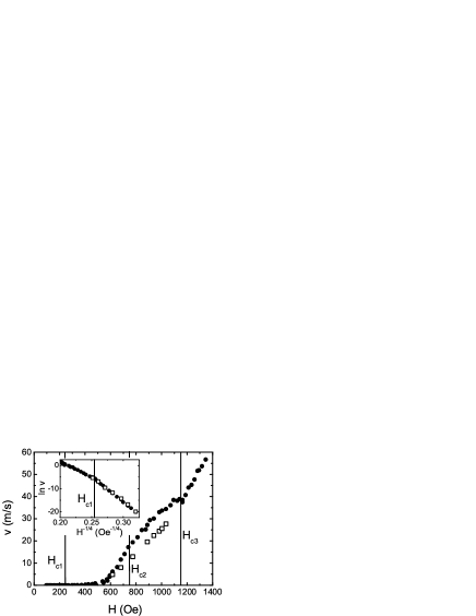
Figure 5: Comparison between experimentally obtained coupled wall dynamics, $v_{\hbox{\tiny C}}(H)$ ($\bullet$), and the theoretically calculated bound state velocity, $v_{b}(H)$ ($\square$).

IV.2 The low field bound state regime

In the creep regime, analytical expressions are available for the wall velocities in the uncoupled case [see Eq. (1)],

$$v_{1}(H)=v_{1}^{0}\exp\left[-\left({a_{1}\over H}\right)^{1\over 4}\right]$$ (12a)

$$v_{2}(H)=v_{2}^{0}\exp\left[-\left({a_{2}\over H}\right)^{1\over 4}\right],$$ (12b)

where experimental values for $v_{i}^{0}$ and $a_{i}$ are given in Table 1.

	Coupling field	exponent	prefactor
	(Oe)	(Oe1/4)	$\ln$(m/s)
Hard (1) layer	$H_{1}=120$	$a_{1}^{1\over 4}=225.2$	$\ln v_{1}^{0}=45.3$
Soft (2) layer	$H_{2}=220$	$a_{2}^{1\over 4}=40.1$	$\ln v_{2}^{0}=10.8$
Bound creep	$-$	$a_{b}^{1\over 4}\approx 202$	$\ln v_{b}^{0}\approx\ln v_{1}^{0}$

Table 1: Experimental values for the coupling field magnitudes and parameters for uncoupled domain wall creep dynamics [Eqs. (12)] as well as bound creep [Eq. (13)].

We are now going to prove that, in the limit $H\to 0$, Eq. (8) has a solution which describes a bound creep motion such that the common domain wall velocity is given by

$$v_{b}(H)=v_{b}^{0}\exp\left[-\left({a_{b}\over H}\right)^{1\over 4}\right].$$ (13)

In order to reduce the notation, let us introduce the quantity $c=f(x)$, which varies in the interval $(-1,+1)$. We have to solve Eq. (8), which using Eqs. (12), can be written as

$$v_{1}^{0}\exp\left[-\left({a_{1}\over H-cH_{1}}\right)^{1\over 4}\right]=v_{2}^{0}\exp\left[-\left({a_{2}\over H+cH_{2}}\right)^{1\over 4}\right].$$ (14)

It is clear that walls must move with a positive velocity, if the external field $H$ is positive. This requires the sign of the total driving fields $H\pm cH_{i}$ to be the same as the sign of $H$, which demands that $c$ vanishes in the limit $H\to 0$. Therefore, we use a small $H$ expansion

$$c=c_{0}H+c_{1}H^{1+\gamma},$$ (15)

where the value of $\gamma$ will be found below, while it is straightforward that the leading term is linear. In fact, if $c$ vanishes faster than linearly, the coupling would not have effect in the limit $H\to 0$ and a bound state would be impossible for small $H$. On the other hand, if $c$ vanishes slower than linearly, $H\pm cH_{i}$ cannot both have the same sign as $H$. In conclusion, using (15) we can rewrite Eq. (14) as

$$v_{1}^{0}\exp\left\{-\left({a_{1}\over H[1-H_{1}(c_{0}+c_{1}H^{\gamma})]}\right)^{1\over 4}\right\}=v_{2}^{0}\exp\left\{-\left({a_{2}\over H[1+H_{2}(c_{0}+c_{1}H^{\gamma})]}\right)^{1\over 4}\right\}\equiv v_{b}^{0}\exp\left[-\left({a_{b}\over H}\right)^{1\over 4}\right],$$ (16)

where we have used the fact that the common speed must have the form (13). Equation (16) can be rewritten as

$$v_{1}^{0}\exp\left[-\left({a_{1}\over H(1-c_{0}H_{1})}\right)^{1\over 4}\left(1-{c_{1}H_{1}\over 1-c_{0}H_{1}}H^{\gamma}\right)^{-1/4}\right]=v_{2}^{0}\exp\left[-\left({a_{2}\over H(1+c_{0}H_{2})}\right)^{1\over 4}\left(1+{c_{1}H_{2}\over 1+c_{0}H_{2}}H^{\gamma}\right)^{-1/4}\right],$$ (17)

which can be approximated, in the limit of vanishing $H$, as

$$v_{1}^{0}\exp\left[-\left({a_{1}\over H(1-c_{0}H_{1})}\right)^{1\over 4}\left(1+{{1\over 4}c_{1}H_{1}\over 1-c_{0}H_{1}}H^{\gamma}\right)\right]=v_{2}^{0}\exp\left[-\left({a_{2}\over H(1+c_{0}H_{2})}\right)^{1\over 4}\left(1-{{1\over 4}c_{1}H_{2}\over 1+c_{0}H_{2}}H^{\gamma}\right)\right].$$ (18)

If we take the logarithm of both sides, we get

$$\ln v_{1}^{0}-\left({a_{1}\over H(1-c_{0}H_{1})}\right)^{1\over 4}\left(1+{{1\over 4}c_{1}H_{1}\over 1-c_{0}H_{1}}H^{\gamma}\right)=\ln v_{2}^{0}-\left({a_{2}\over H(1+c_{0}H_{2})}\right)^{1\over 4}\left(1-{{1\over 4}c_{1}H_{2}\over 1+c_{0}H_{2}}H^{\gamma}\right)\equiv\ln v_{b}^{0}-\left({a_{b}\over H}\right)^{1/4},$$ (19)

which is put in the form of Eq. (13).

The equality in Eq. (19) requires, to leading order in $H$, that

$$\left({a_{1}\over H(1-c_{0}H_{1})}\right)^{1\over 4}=\left({a_{2}\over H(1+c_{0}H_{2})}\right)^{1\over 4}\equiv\left({a_{b}\over H}\right)^{1/4},$$ (20)

that is to say

$${a_{1}\over 1-c_{0}H_{1}}={a_{2}\over 1+c_{0}H_{2}}\equiv a_{b},$$ (21)

which gives

$$c_{0}={a_{2}-a_{1}\over a_{1}H_{2}+a_{2}H_{1}}.$$ (22)

If we replace Eq. (21) in Eq. (19), we get

$$\ln v_{1}^{0}-{{1\over 4}a_{b}^{1/4}c_{1}H_{1}\over 1-c_{0}H_{1}}H^{\gamma-{1\over 4}}=\ln v_{2}^{0}+{{1\over 4}a_{b}^{1/4}c_{1}H_{2}\over 1+c_{0}H_{2}}H^{\gamma-{1\over 4}}\equiv\ln v_{b}^{0}$$ (23)

which has a solution for $c_{1}$ only if $\gamma={1\over 4}$:

$$c_{1}=\frac{\ln\left({v_{1}^{0}\over v_{2}^{0}}\right)}{{1\over 4}a_{b}^{5/4}\left({H_{1}\over a_{1}}+{H_{2}\over a_{2}}\right)}.$$ (24)

Replacing $c_{1}$ in the left or middle expression of (23), we get

$$\ln v_{b}^{0}=\ln v_{1}^{0}-{a_{2}c_{0}H_{1}\over a_{2}-a_{1}}\ln\left({v_{1}^{0}\over v_{2}^{0}}\right).$$ (25)

Using experimental values for separated domain wall velocities, see Tab. 1, we find that $a_{2}/a_{1}\simeq 10^{-3}$ and $H_{1}<H_{2}$, so that (see Eq. (22)), $c_{0}\approx-1/H_{2}$. A negative $c_{0}$ means that walls move at the same speed as a bound state, with the soft wall leading (see Fig. 4). This is expected, because in the uncoupled case, $v_{2}(H)>v_{1}(H)$ for small $H$. Finally, we get

$$a_{b}^{1/4}\simeq 202\hbox{Oe${}^{1/4}$~{}~{}~{}~{}~{}~{}~{}}\ln v_{b}^{0}\simeq\ln v_{1}^{0}.$$ (26)

$a_{b}^{1/4}$ is closer to $a_{1}^{1/4}$ than $a_{2}^{1/4}$ as previously notedMetaxas et al. (2010) and seen in Fig. 3(c). Notably, we can substitute the above creep parameters into Eq. (13) to have a complete analytic expression for the bound state velocity which compares well to the low field $v_{\hbox{\tiny C}}(H)$ data below $H_{c2}$ [see Fig. 6(a)].

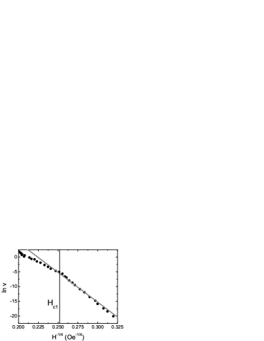
Figure 6: Comparison between experimentally obtained $v_{\hbox{\tiny C}}(H)$ ($\bullet$) and analytical bound state velocity (full line) [Eq. (13) using creep parameters given in Eq. (26)].

IV.3 High field bound state regime

Let us now consider the high field bound state around $H^{*}$. In this regime, comparison between the one-dimensional model and experimental results show only modest agreement. Even if our theory correctly anticipates the existence of a bound state regime around $H=H^{*}$, the agreement between observed ($H_{c2,3}$) and predicted ($H_{c2,3}^{\hbox{\tiny{sf}}}$) limit field values is not perfect. Furthermore, the theory ($v_{b}(H)$) underestimates the experimental ($v_{\hbox{\tiny C}}(H)$) bound state velocity, $v_{b}(H)<v_{\hbox{\tiny C}}(H)$, for $H_{c2}<H<H_{c3}$. Below, we discuss these details and, in particular, why the experimental bound state velocity at $H^{*}$, $v_{\hbox{\tiny C}}(H^{*})\simeq 24.5$m/s, is significantly larger than $v_{1}(H^{*})=v_{2}(H^{*})=v^{*}\simeq 18$m/s. In Appendix B we also give an analytical approximation for the bound state velocity in the high field regime. Finally, it is worth mentioning that the constant distance $x_{0}=x_{2}-x_{1}$ between the soft and the hard walls in the bound regime, is positive for $H<H^{*}$ and negative for $H>H^{*}$ (see Fig. 4), because the leading wall in the bound regime is the wall with the highest speed in the absence of coupling.

Now, let us discuss the disagreement between our theory and experimental results in the high field bound regime. There are three main possibilities to explain this: (1) our coupling model is inadequate, (2) the data used for $v_{2}(H)$ is not representative of the true $v_{2}(H)$ in this system or (3) the use of the experimental $v_{1,2}(H)$ data is not valid for the high field limit.

(1) In Appendix A, we discuss two modifications to the coupling: a dipolar coupling (additional $g(x)$ term in Eqs. (7): see Eqs. (27)) due to strong stray fields at the domain edgesBaruth et al. (2006) and the use of differing $f_{1}(x)$ and $f_{2}(x)$ functions in Eqs. (7) (see Eqs. (28)). However, both modifications still lead to $v_{b}(H^{*})=v^{*}$. Furthermore, since the low field bound regime is well reproduced using only the exchange field, it is questionable to make Eqs. (7) more complicated. One might also consider the case in which $f(x)$ is not continuous. For example, we might have a step function, $f(x)=-1$ for $x<0$ and $f(x)=+1$ for $x>0$. This implies that the bound state is not characterized by a constant distance between walls, but by a continuous interchange between the walls. However, this neither solves the issue surrounding $v_{b}(H^{*})\neq v^{*}$, nor the discrepancy between $H_{c2,3}$ and $H_{c2,3}^{\hbox{\tiny{sf}}}$.

(2) As explained earlier, $v_{2}(H)$ was not measured in this multilayer but rather in a similar one with an equivalent Co(0.5 nm) layer. Using this data, we see that in the vicinity of $H^{*}$, walls in layer 2 exhibit flow motion wherein $v_{2}=mH$ with $m\approx 0.022$ ms^-1Oe^-1. There can be some sample to sample variability however and previous measurements on a single layer Pt/Co(0.5 nm)/Pt filmMetaxas et al. (2007) yielded $m\approx 0.027$ ms^-1Oe^-1. Using this $m$ value to model dynamics in layer 2 for the purpose of determining $v_{b}(H)$ at high field changes $H^{*}$, which is now equal to $H^{*}=910$Oe. The new $m$ value improves the consistency between our calculated $H_{c2}^{\hbox{\tiny{sf}}}$ and $H_{c3}^{\hbox{\tiny{sf}}}$ values (700 Oe and 1070 Oe, respectively) as compared to the experimental values, $H_{c2}$ and $H_{c3}$ (750 Oe and 1150 Oe, respectively). However, the newly calculated value of $v_{b}^{*}$ (24.5 m/s) remains too low with respect to the experimental value $v_{\hbox{\tiny C}}(H^{*}=910\;\hbox{Oe})\simeq 29$m/s Note2 . Note that the film measured in Ref. Metaxas et al., 2007 also had a slightly lower $a^{1/4}$ value (35.1) as compared to $a_{2}^{1/4}$ (40.1, see Table 1), however this has little effect on the predicted bound dynamics since they are dominated by the larger $a_{1}^{1/4}$ value.

(3) Finally, our approach, which works well at low field, may not actually be appropriate at high field where wall dynamics are intrinsically different. At low field, wall motion is thermally activated over field-dependent energy barriers. In contrast, at high field, wall motion is, to a large extent, determined by the internal structure of the wall (and associated internal dynamics) Schryer and Walker (1974); Mougin et al. (2007) which can actually be modified by interlayer coupling Bellec et al. (2010). As such, experimentally obtained, isolated single wall velocities $v_{1}(H)$ and $v_{2}(H)$ may not be the appropriate building blocks to be combined to calculate $v_{b}(H)$, as we did in Eq. (11).

V Conclusion

Exchange coupled Pt/Co layers represent an ideal model experimental system in which to study the interesting problem of coupled interfaces moving through physically separate, but coupled, media. Here we have detailed the principles behind this system and presented both numerical and analytical models of bound domain wall motion which compare well with experimentMetaxas et al. (2010). Most notably, we derive an analytical model with no free parameters which describes bound creep. While we have concentrated on a one dimensional model we hope out results will inspire others to apply micromagneticMartinez et al. (2007); Bellec et al. (2010) or interface modelsKolton et al. (2005, 2009) to this problem.

Appendix A Additional and modified coupling

A more general expression of Eqs. (7) which includes dipolar interactions might be

$$\bar{H}_{1}=H_{1}f(x)+D_{1}g(x)~{}~{}~{}~{}\bar{H}_{2}=-H_{2}f(x)-D_{2}g(x)$$ (27)

where $g(x)=\ln[(d^{2}+x^{2})/d^{2}]$ accounts for dipolar coupling, $d=3$ nm being the separation between the hard and the soft layer. A simple calculationBaruth et al. (2006) can show that in the vicinity of the domain walls, dipolar fields can potentially be larger than $H_{1,2}$. However, as discussed in Sec. IV.3, the good agreement between theoretical and experimental results at low field suggests that it is $H_{1,2}$ which determine the bound state’s stability.

An alternative generalization of Eqs. (7) is to make $f(x)$ different for the two films,

$$\bar{H}_{1}=H_{1}f_{1}(x)~{}~{}~{}~{}\bar{H}_{2}=-H_{2}f_{2}(x).$$ (28)

This might mean, e.g., writing

$$f_{i}(x)=\tanh\left({x\over\Delta_{i}}\right),$$ (29)

with $\Delta_{1}\neq\Delta_{2}$, as is expected for layers with differing thicknessesMetaxas et al. (2007).

However, both of these approaches yield $v_{b}(H^{*})=v^{*}$ since $g(0)=0$ and $f_{1}(0)=f_{2}(0)=0$.

Appendix B Analytical approximation for the high field bound state

In the high field regime, the walls are no longer in the creep regime and Eqs. (12) cannot be used. Instead, we can assume a simple linear approximationLemerle et al. (1998); Metaxas et al. (2007) in the proximity of $H=H^{*}$,

$$v_{i}(H)=v^{*}+\hbox{$\bar{a}_{i}$}(H-H^{*}),$$ (30)

where $v^{*}=v_{i}(H^{*})$ and $\hbox{$\bar{a}_{i}$}\equiv dv_{i}/dH|_{H=H^{*}}$. It can be easily shown that the solution $x=x_{0}$ of Eq. (8) satisfies the relation

$$f(x_{0})=-{(\hbox{$\bar{a}_{1}$}-\hbox{$\bar{a}_{2}$})(H-H^{*})\over\hbox{$\bar{a}_{1}$}H_{1}+\hbox{$\bar{a}_{2}$}H_{2}},$$ (31)

so that

$$v_{b}(H)=v^{*}+\hbox{$\bar{a}_{b}$}(H-H^{*})$$ (32)

with

$$\hbox{$\bar{a}_{b}$}={\hbox{$\bar{a}_{1}$}\hbox{$\bar{a}_{2}$}(H_{1}+H_{2})\over\hbox{$\bar{a}_{1}$}H_{1}+\hbox{$\bar{a}_{2}$}H_{2}}.$$ (33)

Therefore, in the proximity of $H=H^{*}$, the common speed in the high field bound regime is linear, with a slope $\bar{a}_{b}$ which is in between $\bar{a}_{1}$ and $\bar{a}_{2}$:

$$\hbox{$\bar{a}_{2}$}<\hbox{$\bar{a}_{b}$}<\hbox{$\bar{a}_{1}$}.$$ (34)

Using the fitting values $\hbox{$\bar{a}_{1}$}\simeq 0.025$ and $\hbox{$\bar{a}_{2}$}\simeq 0.12$, we find $\hbox{$\bar{a}_{b}$}\simeq 0.035$, so that

$$v_{b}(H)\simeq 18+0.035(H-850),$$ (35)

with $H$ expressed in Oersted and the speed in meters per second.

References

- Lemerle et al. (1998) S. Lemerle, J. Ferré, C. Chappert, V. Mathet, T. Giamarchi, and P. Le Doussal, Phys. Rev. Lett. 80, 849 (1998).
- Repain et al. (2004) V. Repain, M. Bauer, J. P. Jamet, J. Ferré, A. Mougin, C. Chappert, and H. Bernas, Europhys. Lett. 68, 460 (2004).
- Metaxas et al. (2007) P. J. Metaxas, J. P. Jamet, A. Mougin, M. Cormier, J. Ferré, V. Baltz, B. Rodmacq, B. Dieny, and R. L. Stamps, Phys. Rev. Lett. 99, 217208 (2007).
- Kim et al. (2009) K. Kim, J. Lee, S. Ahn, K. Lee, C. Lee, Y. J. Cho, S. Seo, K. Shin, S. Choe, and H. Lee, Nature 458, 740 (2009).
- Paruch et al. (2006) P. Paruch, T. Giamarchi, T. Tybell, and J. M. Triscone, J. Appl. Phys. 100, 051608 (2006).
- Catalan et al. (2008) G. Catalan, H. Béa, S. Fusil, M. Bibes, P. Paruch, A. Barthélémy, and J. F. Scott, Phys. Rev. Lett. 100, 027602 (2008).
- Balankin et al. (2000) A. S. Balankin, A. Bravo-Ortega, and D. M. Matamoros, Phil. Mag. Lett. 80, 503 (2000).
- Blatter et al. (1994) G. Blatter, M. V. Feigel’man, V. B. Geshkenbien, A. I. Larkin, and V. M. Vinokur, Rev. Mod. Phys. 66, 1125 (1994).
- Chauve et al. (2000) P. Chauve, T. Giamarchi, and P. Le Doussal, Phys. Rev. B 62, 6241 (2000).
- Kolton et al. (2009) A. B. Kolton, A. Rosso, T. Giamarchi, and W. Krauth, Phys. Rev. B 79, 184207 (2009).
- Huse and Henley (1985) D. A. Huse and C. L. Henley, Phys. Rev. Lett. 54, 2708 (1985).
- Huse et al. (1985) D. A. Huse, C. L. Henley, and D. S. Fisher, Phys. Rev. Lett. 55, 2924 (1985).
- Kardar (1985) M. Kardar, Phys. Rev. Lett. 55, 2923 (1985).
- Barabasi and Stanley (1995) A. L. Barabasi and H. E. Stanley, Fractal concepts in surface growth (Cambridge University Press, Cambridge, Great Britain, 1995).
- Krusin-Elbaum et al. (2001) L. Krusin-Elbaum, T. Shibauchi, B. Argyle, L. Gignac, and D. Weller, Nature 410, 444 (2001).
- Barabási (1992) A. L. Barabási, Phys. Rev. A 46, R2977 (1992).
- Majumdar and Das (2005) S. N. Majumdar and D. Das, Phys. Rev. E 71, 036129 (2005).
- Juntunen et al. (2007) J. Juntunen, O. Pulkkinen, and J. Merikoski, Phys. Rev. E 76, 041607 (2007).
- Juntunen and Merikoski (2010) J. Juntunen and J. Merikoski, J. Phys.: Condens. Matter 22, 465402 (2010).
- Bauer et al. (2005) M. Bauer, A. Mougin, J. P. Jamet, V. Repain, J. Ferré, R. L. Stamps, H. Bernas, and C. Chappert, Phys. Rev. Lett. 94, 207211 (2005).
- Balankin et al. (2006) A. S. Balankin, R. G. Paredes, O. Susarrey, D. Morales, and F. C. Vacio, Phys. Rev. Lett. 96, 056101 (2006).
- Metaxas et al. (2010) P. J. Metaxas, R. L. Stamps, J.-P. Jamet, J. Ferré, V. Baltz, B. Rodmacq, and P. Politi, Phys. Rev. Lett. 104, 237206 (2010).
- Moritz et al. (2004) J. Moritz, F. Garcia, J. C. Toussaint, B. Dieny, and J. P. Nozières, Europhys. Lett. 65, 123 (2004).
- Wiebel et al. (2005) S. Wiebel, J. P. Jamet, N. Vernier, A. Mougin, J. F. andV. Baltz, B. Rodmacq, and B. Dieny, Appl. Phys. Lett. 86, 142502 (2005).
- Wiebel et al. (2006) S. Wiebel, J. P. Jamet, N. Vernier, A. Mougin, J. Ferré, V. B. B. Rodmacq, and B. Dieny, J. Appl. Phys. 100, 043912 (2006).
- Metaxas et al. (2009) P. J. Metaxas, P. J. Zermatten, J. P. Jamet, J. Ferré, G. Gaudin, B. Rodmacq, A. Schuhl, and R. L. Stamps, Appl. Phys. Lett. 94, 132504 (2009).
- Bustingorry et al. (2008) S. Bustingorry, A. B. Kolton, and T. Giamarchi, Europhys. Lett. 81, 26005 (2008).
- Grolier et al. (1993) V. Grolier, D. Renard, B. Bartenlian, P. Beauvillain, C. Chappert, C. Dupas, J. Ferré, M. Galtier, E. Kolb, M. Mulloy, et al., Phys. Rev. Lett. 71, 3023 (1993).
- (29) K. Fukumoto, W. Kucha, J. Vogel, J. Camarero, S. Pizzini, F. Offi, Y. Pennec, M. Bonfim, A. Fontaine, and J. Kirschner, J. Magn. Magn. Mater. 293, 863 (2005).
- Metaxas et al. (2008) P. J. Metaxas, J. P. Jamet, J. Ferré, B. Rodmacq, B. Dieny, and R. L. Stamps, J. Magn. Magn. Mater 320, 2571 (2008).
- (31) L. San Emeterio Alvarez, K.-Y. Wang, C.H. Marrows, J. Magn. Magn. Mater. 322, 2529 (2010).
- (32) It is easy to prove that the solution and is stable. Otherwise, it would be irrelevant for real dynamics.
- Baruth et al. (2006) A. Baruth, L. Yuan, J. D. Burton, K. Janicka, E. Y. Tsymbal, S. H. Liou, and S. Adenwalla, Appl. Phys. Lett. 89, 202505 (2006).
- (34) Using a different expression for the soft wall velocity implies that the value of the crossing field changes. In our case, Oe for the curves given in Fig. 2(c), while Oe, if m/s.
- Schryer and Walker (1974) N. L. Schryer and L. R. Walker, J. Appl. Phys. 45, 5406 (1974).
- Mougin et al. (2007) A. Mougin, M. Cormier, J. P. Adam, P. J. Metaxas, and J. Ferré, Europhys. Lett. 78, 57007 (2007).
- Bellec et al. (2010) A. Bellec, S. Rohart, M. Labrune, J. Miltat, and A. Thiaville, Europhys. Lett. 91, 17009 (2010).
- Martinez et al. (2007) E. Martinez, L. Lopez-Diaz, O. Alejos, L. Torres, and C. Tristan, Phys. Rev. Lett. 98, 267202 (2007).
- Kolton et al. (2005) A. B. Kolton, A. Rosso, and T. Giamarchi, Phys. Rev. Lett. 94, 047002 (2005).