Effects of Polydispersity and Anisotropy in Colloidal and Protein Solutions: an Integral Equation Approach

Abstract

Application of integral equation theory to complex fluids is reviewed, with particular emphasis to the effects of polydispersity and anisotropy on their structural and thermodynamic properties. Both analytical and numerical solutions of integral equations are discussed within the context of a set of minimal potential models that have been widely used in the literature. While other popular theoretical tools, such as numerical simulations and density functional theory, are superior for quantitative and accurate predictions, we argue that integral equation theory still provides, as in simple fluids, an invaluable technique that is able to capture the main essential features of a complex system, at a much lower computational cost. In addition, it can provide a detailed description of the angular dependence in arbitrary frame, unlike numerical simulations where this information is frequently hampered by insufficient statistics. Applications to colloidal mixtures, globular proteins and patchy colloids are discussed, within a unified framework.

I Introduction

Colloids are dispersions of mesoscopic particles (of the order of 1-500 nm in diameters) suspended in an atomistic fluid. The fact that the typical energy scales involved in their interactions are of the order of the thermal energy, constitutes one of the main differences with respect to simple fluids. An additional important advantage arises from the fact that they allow for an almost arbitrary tunability of interactions (unlike their atomistic counterpart fixed by elementary chemistry), thus opening the possibility of engineering colloidal systems and synthesizing particles with specific properties.

One of the typical difficulties that one has to cope with in the investigation of colloidal suspensions is associated with their polydispersity. As a matter of fact, colloids can hardly be synthetized identical to one another, and they often present a range of different chemical properties, such as size or charge. This fact makes the theoretical analysis of their thermophysical properties rather problematic, a feature that it has been well recognized only in the last decade.

When the distribution of these components is wide, one often approximate it with a continous distribution density, and this is referred to as polydispersity. Physically, the effect of polydispersity is to allow different molecules to pack more closely, thus effectively inhibiting the formation of an ordered structure. As a matter of fact, even within the simple hard-sphere description, there are interesting results, such as, for instance, the disappeareance of a fluid-solid transition for sufficiently large polydispersity. Within simple approximations, (e.g. the Percus-Yevick or the mean-spherical approximations), exact solutions of the Ornstein-Zernike equations are possible for a number of simple but relevant potential models, including hard-spheres, sticky hard-spheres, Coulomb and Yukawa potentials.

Another important fact that has to be taken into account, when dealing with complex fluids, is the possibility of anisotropic interactions.

Isotropic potentials, i.e. potentials that are independent of the relative orientations of the interacting particles, are often exploited in colloidal physics as effective potentials, where the microscopic degrees of freedom are traced out, and thus provide mediated interactions between the larger degrees of freedom. On the other hand, there exists a number of systems where this simplifying approximation is certainly not justified, even at the minimal level. A paramount example of this is given by globular proteins. A protein is physiologically active when the polypeptide chain forming the primary sequence folds into a three-dimensional structure. In spite of the fact that different combinations of the 20 amino acids can, in principle, give rise to a gigantic number of possible different three-dimensional structures, only a few thousand folds have been observed, thus suggesting that a number of strong constraints are drastically limiting the number of possible three-dimensional architectures. Although the globular shape of many proteins could roughly be approximated to a sphere, the presence of different surface groups gives rise to strong anisotropies in the protein-protein interactions.

Another more recent example of anisotropic colloids is given by patchy colloids, which constitutes one recent and very active research topic, in view of the remarkable applications that they might have in the engineering of future materials. Once again, some of the paradigmatic models used in simple fluids can be modified and adapted to the new physical situation. Due to the angular dependence included in the potentials, some of the techniques to be used can be borrowed from the context of associating (molecular) fluids, although important modifications are required in view of the discontinuos nature of the angular dependance that typically occurs in patchy colloids and globular proteins.

This paper aims to review some recent efforts in both directions – polydispersity and anisotropy – that have been carried out in the last few years. While the choice of the topics and the methodologies are mainly dictated by the authors’ interests, it will be shown that in both cases they originated from the landmark studies by Prof. Lesser Blum, that – directly or indirectly — influenced all past, present and future work in the field.

II From Simple to Complex Fluids

For spherically symmetric potentials, thermophysical properties of a system of density $\rho$ can be obtained from the Ornstein-Zernike (OZ) equation

$$h\left(r\right)=c\left(r\right)+\rho\int d\mathbf{r}^{\prime}~{}c\left(r^{\prime}\right)~{}h\left(|\mathbf{r-r}^{\prime}|\right)$$ (1)

but its solution can be accomplished only in the presence of an additional approximation (closure) to the exact relation between the direct correlation function (DCF) $c\left(r\right)$, the potential $\phi(r)$, and the total correlation function $h\left(r\right)$ that has the general form

$$c\left(r\right) = \exp{\left[-\beta\phi\left(r\right)+\gamma\left(r\right)+B\left(r\right)\right]}-1-\gamma\left(r\right)$$ (2)

where $\gamma\left(r\right)=h\left(r\right)-c\left(r\right)$. Here $\beta\equiv\left(k_{\mathrm{B}}T\right)^{-1}$, $k_{\mathrm{B}}$ is Boltzmann’s constant, and $T$ the absolute temperature. The closure may be regarded as an approximation to the bridge function $B(r)$, that is known only as an infinite power series in density whose coefficients cannot be readily calculated (Hansen and McDonald 2006). All practical closures approximate $B\left(r\right)$ in some way.

As a consequence, different routes to achieve structural and thermodynamic quantities yield in general different results, the most well known being the compressibility, the virial (or pressure) and the energy routes (Hansen and McDonald 2006).

Clearly, the goodness of the results depends upon the accuracy of the approximation chosen for the bridge function $B(r)$. Among the most popular approximations are the Mean Spherical Approximation (MSA), with the DCF being related only to the potential outside the core by

$$c\left(r\right)=-\beta\phi\left(r\right)\qquad r\geq\sigma,$$ (3)

complemented by the condition of excluded volume, $h(r)=-1$ inside the hard core of size $\sigma$ (the diameter of a particle); the Percus-Yevick (PY) closure

$$c\left(r\right)=\left[e^{-\beta\phi\left(r\right)}-1\right]\left[1+\gamma\left(r\right)\right],$$ (4)

and the Hypernetted Chain (HNC) closure

$$c\left(r\right)=e^{-\beta\phi\left(r\right)+\gamma\left(r\right)}-1-\gamma\left(r\right)$$ (5)

In the latter the bridge function is set to zero, with the remarkable advantage of having automatically enforced the equality of the virial and the energy routes (Morita 1960). An additional improvement is given by the so-called Reference Hypernetted Chain (RHNC), where the bridge function is taken to be that of the hard-spheres potential with tunable diameter (Lado 1982, 1982a, 1982b). This is selected to reintegrate the energy-virial consistency, lost with the introduction of the bridge function.

In this respect, here we also mention the self-consistent Ornstein-Zernike approximation (SCOZA), a microscopical liquid-state theory that was proposed by Stell and collaborators (Høye and Stell 1977, Pini et al 1998, Kahl et al 2002, Schöll-Paschinger et al 2005, ), that has been shown to be able to predict critical points and lines of the fluid-fluid coexistence with remarkable accuracy. As in the RHNC case, this is a consequence of the enforcing thermodynamic consistency between the different routes.

Unlike simple fluids, complex fluids are typically formed by more than one species and hence the above equations have to be extended to mixtures. As a first example, the case of ionic fluids will be discussed next.

III Long-ranged electrostatic interactions: primitive model for electrolytes

Historically, the first successful theory of ionic solutions was the classic work by Debye and Hückel (1923), based on the solution of the differential Poisson-Boltzmann equation. In the modern work, based upon the statistical mechanics of liquids, ionic fluids are studied by using computer simulations (both Monte Carlo and Molecular Dynamics) or solving some approximate integral equation (IE) for correlation functions, derived from the OZ equation.

The simplest model for electrolyte solutions is the so-called primitive model (PM), in which the ions of species $i$ are depicted as charged hard spheres, with hard sphere (HS) diameter $\sigma_{i}$ and charge $z_{i}e$ ($e$ is the elementary charge, and $z_{i\text{ }}$the electrovalence), embedded in a solvent represented as a continuum with dielectric constant $\varepsilon$. The corresponding interaction potential reads as

$$\phi_{ij}^{\mathrm{PM}}(r)=\left\{\begin{array}[c]{cc}+\infty&r<\sigma_{ij}\equiv(\sigma_{i}+\sigma_{j})/2\\ z_{i}z_{j}e^{2}/\left(\varepsilon r\right)&r\geq\sigma_{ij}\end{array}\right.$$ (6)

and is long-ranged, due to its Coulombic tail added to the HS repulsion term ($i$ and $j$ are species indexes).

The OZ integral equation (1) can then be extended to multicomponent mixtures,

$$h_{ij}(r)=c_{ij}(r)+\sum_{l}\rho_{l}\int d\mathbf{r}^{\prime}\ h_{il}(r^{\prime})c_{lj}(\left|\mathbf{r-r}^{\prime}\right|)$$ (7)

and defines the direct correlation functions $c_{ij}(r)$ in terms of the total correlation functions $h_{ij}(r)\equiv g_{ij}(r)-1$, with $\rho_{l}$ and $g_{ij}(r)$ being respectively the number density of species $l$ and the radial distribution functions (RDF). As in simple fluids, the presence of the HS exclusion between ionic spherical volumes leads to the exact core condition

$$h_{ij}(r)=-1\text{ \ \ \ \ when \ }r<\sigma_{ij}\text{.\ }$$ (8)

Once more, in order to determine both $c_{ij}(r)$ and $h_{ij}(r)$, a second approximate relationship among $h_{ij}(r)$, $c_{ij}(r)$ and $\phi_{ij}(r)$ (a closure) is then required.

The simplest closure useful for ionic fluids is the extension to mixtures of the MSA closure defined in Eq.(3). Although the HNC closure is typically more accurate for ionic fluids, it can be solved only numerically. The main advantage of the MSA is that the OZ-MSA equations can instead be solved analytically.

In the general case of a mixture of charged spheres with arbitrary HS diameters, the analytical MSA solution was obtained by Blum long time ago (Blum, 1975). Such a theory yields both pair correlation functions and thermodynamics in terms of a single parameter $2\Gamma$, which reduces to Debye’s inverse length $\kappa_{\mathrm{D}}$ for dilute ionic solutions. In the MSA the thermodynamic properties are formally similar to those of the Debye-Hückel (DH) theory, but with $\kappa_{\mathrm{D}}$ replaced by $2\Gamma$ (in the MSA theory, the excluded volume effects are more accurately taken into account). In particular, the result for the mean activity coefficient is

$$\ln\gamma_{\pm}=-\frac{\beta e^{2}}{\varepsilon}\ \Gamma\sum_{i}\frac{x_{i}z_{i}^{2}}{1+\sigma_{i}\Gamma}$$ (9)

where $x_{i}$ is the molar fraction of species $i$. The MSA expression for $\ln\gamma_{\pm}$ was used to fit real activity coefficients of some simple electrolytes (Triolo et al., 1977, 1978). Such experimental data were also reproduced by using more refined potentials, different from the PM one. Among these, a model which assumes that solvated ions behave as rigid polarizable charged spheres (Ciccariello, Gazzillo, and Dejak, 1982) and another one where the granular structure of the solvent can also be included to some extent (Ciccariello and Gazzillo, 1982, 1985).

Within the PM potential for ionic fluids, results comparable with the HNC ones can also be obtained by simpler methods. The first one takes into account the first-order perturbative correction in the renormalized cluster expansion of the RDF, while the second approach is based upon an approximation to the Helmholtz free energy coupled with a variational optimization procedure (Ciccariello and Gazzillo, 1983). Remarkably, the DH approximation has been shown to provide consistent energy and virial routes for any potential in any dimensionality (Santos et al, 2009).

Unfortunately, the MSA and all the above-mentioned theories work well only for ions with very small values of the valence $\left|z_{i}\right|$. In real solutions of mesoscopic particles – with sizes within the range $10-10^{4\text{ }}$Å – such as colloids, micelles, and globular proteins, the main difficulties are due to the possible presence of high electric charges and large charge-asymmetries, as well as to the large difference between solute and solvent molecular sizes, thus hampering the utility of these studies within this new context. On the other hand, quite commonly the presence of both the solvent and other electrolytes in the solution can produce a significant screning of all long-ranged electrostatic interactions. Furthermore, due to the large size of the mesoscopic (or macroscopic) suspended molecules, most of the forces acting among them are usually short-ranged, with ranges of only a small fraction of the molecular diameters. Typical examples for nonionic interactions in such fluids are van der Waals attractions, hard-sphere-depletion forces, repulsions among polymer-coated colloids, and solvation effects, including, in particular, hydrophobic bonding and attractions between reverse micelles of water-in-oil microemulsions (Gazzillo et al., 2006a).

In the next section, we then review some results obtained by our group for models of mesoscopic fluids with only short-ranged – both ionic and nonionic – interactions, illustrating also some of their possible biological applications.

IV Short-ranged interactions in fluid systems

From the experimental point of view, several biophysical techniques can be employed for obtaining quantitative data on protein-protein interactions in solution. However, x-ray or neutron small-angle scattering (SAS) stands out for its reliability for studying the whole structure of the solutions and under very different experimental conditions (pH, ionic strength, temperature, etc.).

The SAS intensity divided by the average form factor yields the measurable structure factor (Hansen and McDonald 2006)

$$S_{\mathrm{M}}(q)=\sum_{i,j}\left(x_{i}x_{j}\right)^{1/2}w_{i}(q)w_{j}(q)\ S_{ij}(q),$$ (10)

with

$$w_{i}(q)=\frac{F_{i}(q)}{\sqrt{\sum_{k}x_{k}F_{h}^{2}(q)}},$$ (11)

and where $q$ is the magnitude of the scattering vector, $F_{i}(q)$ the angular average of the form factor of species $i$, and the Ashcroft-Langreth partial structure factors (for spherically-symmetric intermolecular potentials) are given by

$$S_{ij}(q)=\delta_{ij}+4\pi\left(\rho_{i}\rho_{j}\right)^{1/2}\int_{0}^{\infty}dr\,r^{2}h_{ij}(r)\frac{\sin\left(qr\right)}{qr}$$ (12)

in terms of the three-dimensional Fourier transform of $h_{ij}(r)$ ($\delta_{ij}$ being the Kronecker delta).

Theoretical protocols envisage the inverse procedure of the choice of an appropriate potential model to compute correlation functions $h_{ij}(r)$, that can then be used to fit the experimental data with the theoretical scattering intensity via equations (10) and (12).

IV.1 Screened ionic interactions: Yukawa model

In the case of charged protein molecules interacting via screened Coulomb forces, a simple model can be obtained by adding to a HS repulsion term a tail (for $r\geq\sigma_{ij}$) given by the Yukawa potential

$$\phi_{ij}^{\text{Y}}(r)=\frac{z_{i}z_{j}e^{2}}{\varepsilon(1+\kappa_{D}\sigma_{i}/2)(1+\kappa_{D}\sigma_{j}/2)}\ \frac{\exp[-\kappa_{D}(r-\sigma_{ij})]}{r},$$ (13)

which represents an effective interaction between two isolated macroions in a sea of microions. The functional form is the same as in the DH theory of electrolytes, but the coupling coefficients are of the well-known DLVO (Derjaguin-Landau-Vervey-Overbeek) type (Vervey and Overbeek 1948). Here, the inverse Debye screening length $\kappa_{D}$ is due only to microions, i.e.

$$\kappa_{D}=\sqrt{\frac{8\pi\beta e^{2}}{\varepsilon}\frac{N_{A}}{1000}\left(I_{c}+I_{s}\right)},$$ (14)

where $N_{A}$ is the Avogadro number, and $I_{c}=(1/2)c_{c}z_{c}^{2}$ denotes the ionic strength of the counterions originated from the ionization of the protein macromolecules ($c_{c}$ being the molar concentration of these counterions), while $I_{s}=(1/2)\sum_{i}c_{i}^{\mathrm{micro}}\left(z_{i}^{\mathrm{micro}}\right)^{2}$ is the ionic strength of all microions (cations and anions) generated by added salts. Clearly, $\kappa_{D}^{-1}$ is temperature-dependent and indicates the range of the screened Coulomb interactions: $\kappa_{D}\rightarrow 0$ corresponds to pure Coulomb potentials, while $\kappa_{D}\rightarrow\infty$ yields the opposite HS limit.

For a general HS-Yukawa (HSY) model

$$\phi_{ij}^{\mathrm{HSY}}(r)=\left\{\begin{array}[c]{cc}+\infty&r<\sigma_{ij}\\ A_{i}A_{j}\exp[-z(r-\sigma_{ij})]/r\text{ \ \ }&r\geq\sigma_{ij}\end{array}\right.,$$ (15)

Blum et al. (Blum and Høye, 1978; Ginoza, 1990) found an analytical solution of the OZ equations, again within the MSA closure. Nevertheless, under common experimental regimes corresponding to low density and strong electrostatic repulsions (weak screening), the MSA displays a serious drawback, since RDFs may assume unphysical negative values close to the contact distance $\sigma_{ij}$, for particles $i$ and $j$ which repel each other. To overcome this shortcoming for repulsive Yukawa models, one has to resort to different closures. In general then, only numerical solutions are feasible, and thus IE algorithms can hardly be included into best-fit programs for the analysis of SAS results. The use of analytical solutions, or simple approximations requiring only a minor computational effort, is clearly much more advantageous when fitting experimental data.

The HSY model was employed for instance in the interpretation of Small-Angle-X-ray Scattering (SAXS) measurements on structural properties of a particular globular protein, the $\beta$-lactoglobulin ($\beta$LG), in acidic solutions (pH = 2.3) at several values of ionic strength in the range 7-507 mM (Baldini et al 1999, Spinozzi et al 2002). In particular, this protein clearly exhibits a monomer-dimer equilibrium, affected by the ionic strength of the solution. A “two-component macroion model”, with repulsive HSY interactions between two species with charges of the same sign (mimicking both monomers and dimers of $\beta$LG), was shown to provide a remarkable good description of the above-mentioned SAXS data (Spinozzi et al 2002). The crucial feature of that study was the proposal of a relatively simple approximation to the RDFs, requiring a little computational effort and thus suitable for best-fit programs, and applicable to other spherically-symmetric potentials. We review here the main idea.

The RDF can be expressed exactly in terms of the potential of mean force $W_{ij}(r)$ as

$$g_{ij}(r)=\exp\left[-\beta W_{ij}(r)\right].$$ (16)

In the zero-density limit $\rho\rightarrow 0$, $W_{ij}(r)$ reduces to the potential and $g_{ij}\left(r\right)$ thus becomes the Boltzmann factor $g_{ij}\left(r\right)=\exp\left[-\beta\phi_{ij}\left(r\right)\right]$. This zeroth-order (W0) approximation was frequently used in the analysis of experimental scattering data, since it avoids the problem of solving the OZ equations, but is largely inaccurate except, perhaps, at extremely low densities. Its first-order perturbative correction (W1-approximation) reads (Spinozzi et al 2002)

$$g_{ij}\left(r\right)=\exp\left[-\beta\phi_{ij}\left(r\right)+\omega_{ij}^{(1)}(r)\rho\right],$$ (17)

with $\omega_{ij}^{(1)}(r)$ given by

$$\omega_{ij}^{(1)}(r)=\sum_{l}{x_{l}}\int\mathrm{d}\mathbf{r}^{\prime}~{}f_{il}\left(r^{\prime}\right)~{}f_{lj}\left(|\mathbf{r-r}^{\prime}|\right).$$ (18)

These convolution integrals of the Mayer functions

$$f_{ij}\left(r\right)=\exp\left[-\beta\phi_{ij}\left(r\right)\right]-1$$ (19)

can be easily calculated in bipolar coordinates. It is worth noting that this W1-expression for $g_{ij}\left(r\right)$ is never negative, thus overcoming the major drawback of MSA (the monomer effective charge resulting from the fit falls near $20e$). As expected, the W1-approximation largely improves the fit with respect to the W0-one (Spinozzi et al., 2002).

A test of W1 against MC simulations confirmed that the first-order approximation W1 is valid for the considered system even at strong Coulomb coupling, provided that the screening is not too weak, i.e. for Debye length smaller than monomer radius (Giacometti et al., 2005).

An example of these results (Giacometti et al., 2005) is depicted in Figure 1 where the three components $g_{ij}(r)$ are computed from numerical simulations under the experimetal conditions studied in (Spinozzi et al 2002), and compared with integral equation theory (PY and HNC) and W1 approximation.

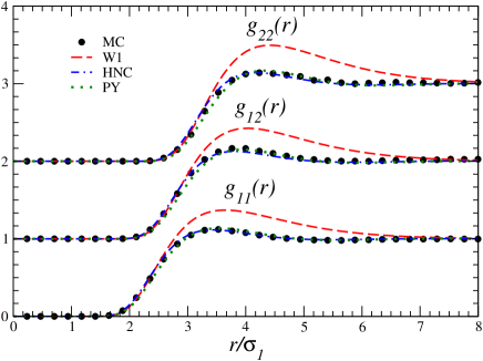
Figure 1: (Color online) Plot of the $g_{11}(r)$, $g_{12}(r)$, $g_{22}(r)$ for a Yukawa potential. Points refer to MC simulations carried out under relevant experimental conditions Spinozzi02 , and compared with integral equations (PY dotted line, HNC dash-dotted line) and with the first-order W1 expansion (dashed line).

IV.2 Nonionic surface interactions: adhesive hard sphere model

In colloidal suspensions of neutral mesoscopic molecules, attractive forces working at very short distances are quite common. These interactions may stem from van der Waals (or dispersion) attractions between induced dipoles, depletion forces in colloid-polymer mixtures, solvation effects, hydrophobic bonding, and so on (Gazzillo et al., 2006a).

The simplest model mimicking these very short-ranged attractive interactions is the “adhesive” or “sticky” hard spheres (SHS), which adds to a HS interparticle repulsion an infinitely strong attraction when the molecular surfaces come to contact. Baxter proposed the one-component version of this model, solved the OZ equation with the PY closure, and found that such a system presents a liquid-gas phase transition (Baxter, 1968). The adhesive surface contribution is defined by a particular limiting case of a square-well (SW) tail, in which the depth goes to infinity as the width goes to zero, in such a way that the contribution to the second virial coefficient $B_{2}$ remains finite and different from zero (Baxter’s “sticky limit”). More explicitly, in the one-component case, one starts from the particular SW potential

$$\phi^{\mathrm{Baxter}\text{ }\mathrm{SW}}(r)=\left\{\begin{array}[c]{cc}+\infty&r<\sigma\\ -\epsilon\equiv-\beta^{-1}\ln\left(1+\frac{t}{\Delta}\right)\text{ \ \ \ \ \ }&\sigma\leq r<R\equiv\left(1+\Delta\right)\sigma\\ 0&r\geq R\end{array}\right.$$ (20)

where $\epsilon>0$ and $w\equiv R-\sigma=\Delta\cdot\sigma$ denote the depth and the width of the SW, respectively, while $t$ is simply related to Baxter’s original parameter $\tau$ by

$$t=\frac{1}{12\tau}$$ (21)

Here, $t$ measures the strength of surface adhesiveness or “stickiness” between particles, and is an unspecified decreasing function of $T.$ In fact, as $T\rightarrow\infty$ one must get $\tau\rightarrow\infty$, in order to recover the correct limit corresponding to a HS fluid.

For this SW potential, the Mayer function and the second virial coefficient become

$$f^{\ \mathrm{Baxter}\text{ }\mathrm{SW}}(r)=\left\{\begin{array}[c]{ll}-1&\qquad 0<r<\sigma\\ t\ \Delta^{-1}&\qquad\sigma\leq r\leq R\\ 0&\qquad r\geq R\end{array}\right.,$$ (22)

$$B_{2}^{\ \mathrm{Baxter}\text{ }\mathrm{SW}}=-2\pi\int_{0}^{\infty}dr\ r^{2}f(r)=\frac{2\pi}{3}\sigma^{3}\left\{1-\frac{t}{\Delta}\left[\left(1+\Delta\right)^{3}-1\right]\right\},$$ (23)

respectively. Taking the “sticky limit” $\Delta\rightarrow 0$, the Mayer function becomes

$$f^{\ \mathrm{SHS}}(r)=\left[\Theta\left(r-\sigma\right)-1\right]+t\ \sigma\ \delta\left(r-\sigma\right)$$ (24)

with $\Theta(x)$ being the Heaviside function ($=0$ when $x<0$, and $=1$ when $x>0$) and $\delta(x)$ the Dirac delta function, while the SHS second virial coefficient is simply

$$B_{2}^{\mathrm{SHS}}=B_{2}^{\mathrm{HS}}\left(1-3t\right)=\frac{2\pi}{3}\sigma^{3}\left(1-\frac{1}{4\tau}\right).$$ (25)

Here $B_{2}^{\mathrm{HS}}=2\pi\sigma^{3}/3$ is the second virial coefficient of hard-spheres. The surface adhesion corresponds to the term $t\ \sigma\ \delta\left(r-\sigma\right)$, where the Dirac $\delta$ ensures that the interaction occurs only at contact, i.e. when $r=\sigma.$

Although it is known that SHSs of equal diameter, when treated exactly rather than in the PY approximation, are not thermodynamically stable (Stell 1991), the SHS-PY solution, both for the one-component case and for mixtures, has nevertheless received a continuously growing interest in the last decades as a useful model for colloidal suspensions, micelles, microemulsions and globular protein solutions, mainly because of its capability to exhibit a gas-liquid phase transition.

In addition to Baxter’s model and its PY solution (that hereafter will be referred to as SHS1 model and SHS1-PY solution, respectively), more than two decades ago some authors proposed an alternative definition of adhesive-hard-sphere model, starting from the particular HSY potential

$$\beta\phi^{\mathrm{HSY}}(r)=\left\{\begin{array}[c]{cc}+\infty&r<\sigma\\ -zK_{0}\exp[-z(r-\sigma)]/r\text{ \ \ }&r\geq\sigma\end{array}\right.$$ (26)

and performing a “sticky limit”, which in this case amounts to taking $z\rightarrow+\infty$. The resulting model (denoted as SHS2) admits an analytic solution within the MSA closure, and this SHS2-MSA solution is somehow simpler than the original SHS1-PY one. Consequently, several authors utilized the SHS2-MSA solution, under the – implicit or explicit – assumption that both the SHS1 and SHS2 model were different but equivalent representations of a unique SHS potential. Unfortunately, this turns out not to be the case, and the usage of both the above-mentioned models has generated some confusion in the past. The problem is not simply that the SHS2-MSA is a different solution, but – more drastically – that, unlike SHS1, the SHS2 model itself is not well defined (Gazzillo and Giacometti, 2003a), as the exact second virial coefficient of the HSY potential diverges in the sticky limit $z\rightarrow+\infty$.

Within the MSA, this pathology of the SHS2 model is masked by the closure, at least in the SHS2-MSA compressibility equation of state (EOS), whereas both the virial and the energy MSA pressures of the HSY fluid diverge in the sticky limit (Gazzillo and Giacometti, 2003a).

Gazzillo and Giacometti (2003a) introduced a simple alternative model (SHS3), in such a way that the exact $B_{2}$ remains finite in the sticky limit, and yet the OZ equations can still be analytically solved within a new closure (the modified MSA, or mMSA). Rather interestingly, the SHS3-mMSA solution has exactly the same formal expression as the SHS2-MSA one and this remarkable equivalence allows to recover all previous results for structure factors and compressibility EOS based upon the SHS2-MSA solution, after an appropriate re-interpretation.

V Polydispersity

Polydispersity is a rather common feature in both ionic and nonionic suspensions of colloids and micelles. It means that mesoscopic suspended particles of a same chemical species are not necessarily identical, but some molecular properties (size, charge, etc.) may exhibit a discrete or continuous distribution of values. Thus, even when all macroparticles belong to a unique chemical species, a polydisperse fluid is practically a multicomponent mixture, with a very large number $p$ of components – of order $10^{1}\div 10^{3}$ or more (discrete polydispersity) – or with $p\rightarrow\infty$ (continuous polydispersity).

In a fluid of spherical molecules with polydispersity only in size, each component of the mixture is characterized by a different diameter. In the case of discrete polydispersity, one can specify a large set of possible diameters $\left\{\sigma_{i}\right\}$ (with $i=1,\ldots,p$) and the molar fractions $\left\{x_{i}\right\}$ of the corresponding components. In the continuous case, all diameters $\sigma\geq 0$ must be included and the discrete molar fractions must be replaced by a continuous distribution, according to the following substitution rules

$$\begin{array}[c]{c}x_{i}\rightarrow dx=f\left(\sigma\right)d\sigma\\ \sum_{i}x_{i}\ \ldots\rightarrow\int d\sigma\ f\left(\sigma\right)\ \ldots\end{array}$$ (27)

where $f\left(\sigma\right)d\sigma$ is the probability of finding a particle with diameter in the range $\left(\sigma,\sigma+d\sigma\right)$, and the distribution function $f\left(\sigma\right)$ (molar fraction density function) is normalized.

A common, but not unique, choice for $f\left(\sigma\right)$ is the Schulz (or gamma) distribution (see Fig. 2)

$$f\left(\sigma\right)=\frac{b^{a}}{\Gamma\left(a\right)}\ \sigma^{a-1}e^{-b\sigma}\text{ \ \ (}a>1\text{),}$$ (28)

where $\Gamma$ is the gamma function, and the two parameters $a$ and $b$ can be expressed as $a=1/s^{2}$ and $b=a/\left\langle\sigma\right\rangle$, in terms of the mean value $\left\langle\sigma\right\rangle$ and the relative standard deviation $s\equiv\sqrt{\left\langle\sigma^{2}\right\rangle-\left\langle\sigma\right\rangle^{2}}/\left\langle\sigma\right\rangle$. The dispersion parameter $s$, varying in the range $(0,1)$, measures the degree of polydispersity (typical experimental values of $s$ lie in the range $0\div 0.3$). When $s\rightarrow 0$ the Schulz distribution reduces to a Dirac $\delta$ centered at $\left\langle\sigma\right\rangle$ (monodisperse limit), for small $s$ values $f\left(\sigma\right)$ is very similar to a Gaussian distribution (without its drawback of unphysically negative diameters) and finally, for $s$ closer to $1$, $f\left(\sigma\right)$ becomes asymmetric, with a long tail at large diameters.

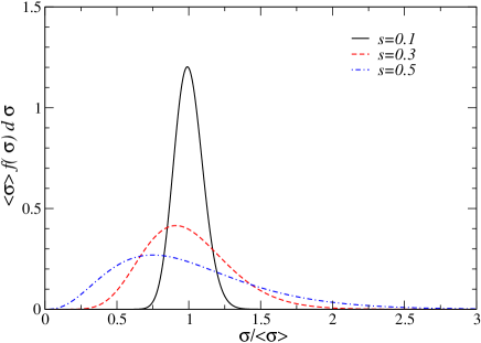
Figure 2: (Color online) Plot of the Schultz distribution for different values of the polydispersity parameter $s$.

In the presence of polydispersity the interpretation of experimental measurements is a hard task, as polydispersity can significantly affect the microscopic structure of mesoscopic fluids, and must thus be taken into account in the analysis of their SAS or thermodynamic data. Unfortunately, polydispersity and large size and/or charge asymmetries represent a serious challenge to the available theoretical tools, such as MC or molecular dynamics simulations as well as to integral equations.

V.1 Effects on the structure factor

If one is interested in the static structural properties of polydisperse fluids, then the measurable structure factor $S_{\mathrm{M}}(q)$ for x-ray, neutron or light SAS is usually considered, as already remarked.

Blum pionieered the first theoretical attempts in this context, by obtaining a closed analytical expression for the scattering intensity from a HS mixture, valid for any number $p$ of components and even in the case of continuous size polydispersity (Vrij, 1978; Blum and Stell, 1979).

Building upon these fundamental contributions, an extension of these calculations to ionic fluids was subsequently proposed (Gazzillo et al., 1997). Approximate scattering functions for polydisperse ionic colloidal fluids were also obtained by a corresponding-states approach, originally proposed for non-ionic polydisperse mixtures (Gazzillo et al., 1999a, 1999b; Carsughi et al., 2000). For simplicity, the charge polydispersity of the macroions was assumed to be fully correlated to their size polydispersity, as the charge (or valence) of each macroion was set to be proportional to its surface area, i.e.

$$z\left(\sigma\right)=z_{\left\langle\sigma\right\rangle}\left(\frac{\sigma}{\left\langle\sigma\right\rangle}\right)^{2},$$ (29)

where $z_{\left\langle\sigma\right\rangle}$ denotes the valence of the macroions having diameter $\left\langle\sigma\right\rangle$.

Ginoza and Yasutomi (1998a, 1998b) obtained analytical expressions for the structure factor of colloidal dispersions with screened Coulomb interactions, in the presence of both size and charge polydispersities. They utilized the MSA solution for multicomponent HSY fluids, and analyzed experimental data for a salt-free acqueous suspension of highly charged polystyrene spheres ($z\approx 273e$). These authors also studied the equation of state and other thermodynamic properties of polydisperse colloidal suspensions, again with the HSY model (Ginoza and Yasutomi, 1997, 1998c).

Additional studies by our group unraveled the structure of polydisperse sticky hard spheres in some details (Gazzillo and Giacometti, 2000, 2002, 2003b, 2004).

From a general qualitative point of view, the effect of polydispersity on the structure factor of a mixture is threefold, both for ionic and nonionic fluids. As $s$ is increased at fixed packing fraction $\eta$, i) the value of $S_{\mathrm{M}}(q=0)$ is increased, since highly dispersed particles can be more efficiently packed; ii) the first peak is lowered, broadened and shifted to smaller $q$ values, corresponding to a larger distance between nearest-neighbour molecules; iii) the oscillations on the tail of the curves, and thus the range of microscopic ordering, are greatly reduced, as a consequence of the destructive interference stemming from the several length scales involved (see Figure 3).

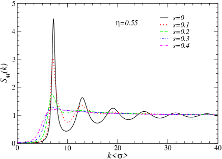
Figure 3: (Color online) Plot of the effective structure factor $S_{M}(k)$ as a function of $k\langle\sigma\rangle$ for hard sphere potential and different polydispersity degrees.

V.2 Effects on phase behaviour

Our group also addressed the phase behaviour of polydisperse (or even binary) SHS fluids extensively, focusing on stability boundaries, percolation threshold (related to flocculation) gas-liquid coexistence with its cloud and shadow curves, and size fractionation effects (Fantoni et al., 2005a, 2005b, 2006; Gazzillo et al., 2006b). We considered several different cases of polydispersity, so that for a complete description of the results we refer to the original papers. As a general rule, the main findings are that i) polydispersity inhibits instabilities, i.e. the mixture becomes more stable with respect to concentration fluctuations; ii) polydispersity increases the region of the phase diagram where the fluid is not percolating, and iii) it diminishes the size of the two-phase coexistence region.

VI Anisotropy effects

VI.1 Failure of isotropic models for globular proteins

Until few years ago, it was widely accepted that the crucial problem to be addressed in the framework of colloidal solutions was, as remarked, the effect of polydispersity. This view has however been challenged recently, as a significant leap forward has been performed in the chemical syntesis of colloidal particles (Hong et al 2008). Today there exist a number of well defined experimental protocols to produce a wide variety of colloidal particles with diverse anisotropies in shape, chemical composition, functionality, and surface make-up (Walther and Müller 2000, Pawar and Kretzschmar 2010).

Even on the protein side, however, the use of spherically symmetric potentials to describe protein-protein interactions at the tertiary level, has long ago been proven to be inadequate. This holds true both for numerical simulations (such as Monte Carlo or molecular dynamic simulations) and integral equation theories. While difficulties in the extension of the former to anisotropic potentials is mainly due to the enormous increase of computational time that requires the use of clever techniques to maintain it within an affordable range, in the latter case a significant extension of the theoretical formalism is also necessary. As it will be further elaborated below, some of these models can be also tackled with standard analytical tools, although the success of these attempts has been so-far limited to qualitative agreements. These models and techniques are typically adapted from those devised for molecular fluids (Gray and Gubbins 1984, Hansen and McDonald 2006).

There are two additional pieces of information that can be given at this point. Firstly, that RHNC provides a rather precise description of both structural and thermodynamical properties arising from typical isotropic potentials such as, for instance, the square-well (SW), as it appears from a detailed comparison with MC simulations. This was illustrated recently by a detailed analysis that addressed specifically the derivation of the gas-liquid coexistence curve (binodal) using integral equations (Giacometti et al 2009a). Rather surprisingly, in spite of the large number of studies applying integral equation theory to SW, only two other examples of these calculations, both very recent and with different closures, are known in the literature, to the best of our knowledge (White and Lipson 2007, El Mendoub et al 2008).

Secondly, none of the isotropic potentials can capture some of the essential features of globular proteins in solutions. as illustrated by a comparison with small-angle-scattering experiments. This second point was inferred through a dedicated study that compared experimental results stemming from small-angle-scattering to MC simulations and integral equations (PY and HNC) for Yukawa potentials (Giacometti et al 2005).

VI.2 Patchy and dipolar-like models

We now analyse some of the theoretical models that have been recently discussed in this framework. The selection is only meant to be representative and largely influenced by the interests of the authors in the field.

Let us focus on one of the experimental techniques, called templating, that has proven to be one of the most efficient to directly access to the surface of a colloidal particle and modify its functionality in a controlled and heterogeneous way (Hong et al 2008). In this paper, the authors exploited the so-called Pickering technique, that is an efficient way of trapping colloidal particles at an emulsion interface, combined with epifluorescence microscopy, that is a useful tool to visualize them, to obtain a set of amphiphilic colloidal particles where one of the two hemispherical surfaces is hydrophobic and the other is charged. If the division is even ($50\%$ hydrophobic and $50\%$ charged), these spheres are a nice example of the so-called Janus particles. When Janus particles are inserted into pure water, they tend to form isolated monomers irrespective of their orientation, because of the strong repulsions. One the other hand, one can screen the repulsion by adding suitable salt, so that clusters with complex morphologies can be obtained depending on the salt concentration.

An interesting minimal model to tackle this problem was proposed by Kern and Frenkel (2003) patterned after a similar model introduced by Chapman, Jackson and Gubbins (Chapman et al 1988) in the framework of molecular fluids.

The Kern-Frenkel potential reads

$$\Phi\left(12\right) = \phi\left(r_{12}\right)\Psi\left(\hat{\mathbf{n}}_{1},\hat{\mathbf{n}}_{2},\hat{\mathbf{r}}_{12}\right),$$ (30)

where the radial part is a SW potential

$$\phi\left(r\right)=\left\{\begin{array}[]{ccc}\infty,&&0<r<\sigma\\ -\epsilon,&&\sigma<r<\lambda\sigma\\ 0,&&\lambda\sigma<r\end{array}\right.$$ (31)

and the angular part is given by

$$\Psi\left(12\right)\equiv\Psi\left(\hat{\mathbf{n}}_{1},\hat{\mathbf{n}}_{2},\hat{\mathbf{r}}_{12}\right)=\left\{\begin{array}[]{ccccc}1,&\text{if}&\hat{\mathbf{n}}_{1}\cdot\hat{\mathbf{r}}_{12}\geq\cos\theta_{0}&\text{and}&-\hat{\mathbf{n}}_{2}\cdot\hat{\mathbf{r}}_{12}\geq\cos\theta_{0},\\ 0,&&&\text{otherwise},&\end{array}\right.$$ (32)

$\theta_{0}$ being the angular semi-amplitude of the patch. Here $\hat{\mathbf{n}}_{1}(\omega_{1})$ and $\hat{\mathbf{n}}_{2}(\omega_{2})$ are unit vectors giving the directions of the center of the patch in spheres 1 and 2, respectively, with $\omega_{1}=(\theta_{1},\varphi_{1})$ and $\omega_{2}=(\theta_{2},\varphi_{2})$ being their corresponding spherical angles in an arbitrarily oriented coordinate frame. Similarly, $\hat{\mathbf{r}}_{12}(\Omega)$ is the unit vector of the separation $\mathbf{r}_{12}$ between the centers of mass of the two spheres, and is defined by the spherical angle $\Omega$. As usual, we have denoted with $\sigma$ and $(\lambda-1)\sigma$ the hard core diameter and the width of the well.

The coverage $\chi$ is defined by the fraction of attractive surface, that is

$$\chi = \left\langle\Psi\left(\hat{\mathbf{n}}_{1},\hat{\mathbf{n}}_{2},\hat{\mathbf{r}}_{12}\right)\right\rangle_{\omega_{1}\omega_{2}}^{1/2}=\sin^{2}\left(\frac{\theta_{0}}{2}\right).$$ (33)

where we have defined $\langle\ldots\rangle_{\omega}=(4\pi)^{-1}\int d\omega\ldots$ as the angular average over the solid angle $\omega$.

The three most relevant configurations for the Janus case ($\chi=0.5$) are depicted in Figure 4. The color coding in this figure is that green (light gray) corresponds to the SW part, whereas red (dark grey) to the HS part. The left panel depicts the head-to-head configuration, where the two patches are perfectly facing one another, and hence attraction is identical to the SW counterpart. The central panel, corresponds to the perperdicular case, where there is a partial overlapping, whereas the right panel displays the head-to-tail configuration, where there is no binding even at contact.

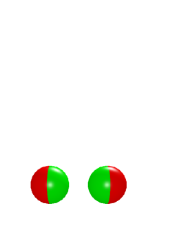
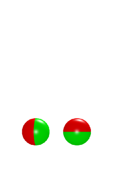
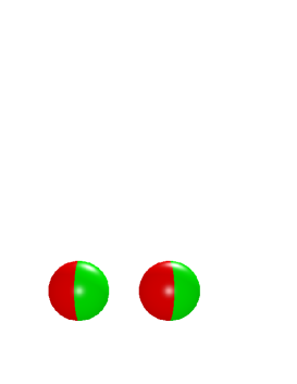
Figure 4: (Color online) Typical configurations for the Kern-Frenkel potentials under $50\%$ coverage (Janus particle $\chi=0.5$). From left to right: head-to-head, perpendicular and head-to-tail alignment. The color coding is the following: light grey (green), attractive part; dark grey (red) repulsive part.

Hinging upon the SW radial counterpart, this model cannot be easily tackled by analytical means. A more convenient model for analytical treatment was suggested by Fantoni et al (2007) and is an extension of the SHS to angular dependent interactions where the Boltzmann factor has the following expression

$$e\left(12\right) = \Theta(r_{12}-\sigma)+\frac{\Psi\left(12\right)}{12\tau}\sigma\delta(r_{12}-\sigma)~{}.$$ (34)

When $\Psi(12)=1$ we recover the usual Baxter SHS model (see Eq.(24)) and hence the only orientational dependence is included into the definition of $\Psi(12)$. In very much the same way as it happens to the Kern-Frenkel potential, this reduces to the usual SW interaction in the limit $\Psi(12)=1$, obtained whenever the fraction of surface pertaining to the SW attractive potential (i.e. the coverage) tends to $1$, and hence $\theta_{0}\to\pi$. The physical meaning of the above equations is rather clear. In both cases the original spherical model has been extended to include an angular dependence that reduces the overall attraction. As we shall see, this has far reaching consequences for the resulting gas-liquid phase diagram.

Another possibility is to include continuous modulation, as opposite to reduction, of the attraction. Within the SHS framework, this can be done, for instance, by the following Boltzmann factor (Gazzillo et al 2008, 2009, Gazzillo 2010, 2011)

$$e(12)=e_{\mathrm{HS}}(r)+t\ \epsilon(1,2)\ \sigma\delta\left(r_{12}-\sigma\right),$$ (35)

$$\epsilon(1,2)=1+\alpha D(1,2),$$ (36)

where $\alpha$ is a tunable parameter, and where we have defined the dipolar function

$$D(12)=D\left(\hat{\mathbf{r}}_{12},\hat{\mathbf{n}}_{1},\hat{\mathbf{n}}_{2}\right)=3(\hat{\mathbf{r}}_{12}\cdot\hat{\mathbf{n}}_{1})(\hat{\mathbf{r}}_{12}\cdot\hat{\mathbf{n}}_{2})-\hat{\mathbf{n}}_{1}\cdot\hat{\mathbf{n}}_{2}$$ (37)

Note that this potential can be reckoned as the analog of the dipolar potential without its radial dependence, which is here of the SHS type. As such, the attractive part in this potential is not reduced, but only redistributed in an asymmetric way along the various directions.

VII Analytical approaches and integral equation theories

As anticipated, the case of angular dependent potentials turns out to be far more challenging for theoretical approaches as compared with their symmetrical counterparts, so that only very highly simplified models are actually accessible. We now review some of them into a unified perspective.

VII.1 Virial expansion

The virial expansion has the following general form

$$\frac{\beta P}{\rho} = 1+B_{2}\left(T\right)\rho+B_{3}\left(T\right)\rho^{2}+\ldots$$ (38)

For the variation of the Kern-Frenkel potential, given in Eq.(34), the first two virial coefficients are (Fantoni et al, 2007)

$$B_{2} = \left(\frac{\pi\sigma^{3}}{6}\right)\left[4-12\frac{\chi_{1}}{12\tau}\right]~{},$$ (39)

$$B_{3} = \left(\frac{\pi\sigma^{3}}{6}\right)^{2}\left[10-60\frac{\chi_{1}}{12\tau}+144\frac{\chi_{2}}{(12\tau)^{2}}-96\frac{\chi_{3}}{(12\tau)^{3}}\right]~{},$$ (40)

where $\chi_{1}$, $\chi_{2}$ and $\chi_{3}$ are terms accounting for the actual reduction of the coverage angle $\theta_{0}$ and are thus related to it. Explicit expressions of them, as a function of $\theta_{0}$, can be found in Fantoni et al (2007).

It is worth emphasizing that if one limits the expansion to the second virial coefficient, a law of corresponding states based on the rescaling $\tau\rightarrow\tau/\chi_{1}$ between the patchy and the isotropic SHS models holds true, and this could also be connected with the SW counterpart by computing the corresponding second virial coefficient. However, this correspondence breaks down even at the level of the third virial coefficient, as shown in equations (40). This clearly holds true even more for the SW case, where the second virial coefficient is not linearly related with temperature.

As in spherical potentials, the most reliable approach hinges upon integral equation theories that will be discussed next.

VII.2 Angular-dependent Ornstein-Zernike equation and closure

The more general case of SW potential for the radial part cannot be tackled analytically so one has to resort to either numerical simulations or integral equation theories. The implementation of both turns out to be not an easy task in the case of angular dependent potentials.

Let us here focus on the latter, where the OZ equation in terms of $\gamma(12)=h(12)-c(12)$ is the generalization of Eq.(1) to angular dependent potentials

$$\gamma\left(12\right) = \frac{\rho}{4\pi}\int d\mathbf{r}_{3}d\omega_{3}\left[\gamma\left(13\right)+c\left(13\right)\right]c\left(32\right),$$ (41)

while the general form of a closure is again a generalization of Eq.(2)

$$c\left(12\right) = \exp\left[-\beta\Phi\left(12\right)+\gamma\left(12\right)+B\left(12\right)\right]-1-\gamma\left(12\right).$$ (42)

The additional procedure for implementing integral equations for angular dependent potentials is constituted by an expansion in spherical harmonics and by rotations among different frames through Clebsh-Gordan transformations (Gray and Gubbins 1984).

The great advantage of integral equation theory with respect to numerical simulations is that a complete description of any correlation functions can be given in any frame, within the chosen closure. This allows to uncover some nuances that are not easily seen in numerical simulations, in view of the fact that some sort of angular averages have to be performed in order to achieve a reasonable statistics.

VIII Effects on the thermodynamics and structural properties

The Kern-Frenkel potential described in Eqs.(30)-(32) can be regarded as an intermediate case, bracketed by a fully isotropic SW potential (corresponding to $\theta_{0}=\pi$, or $\chi=1$) and a hard-sphere potential ($\theta_{0}=0$, or $\chi=0$). Hence this anisotropic model smoothly interpolates between two well known and studied isotropic fluids that can then be used as benchmarks. The main effect of the anisotropy is the reduction of the global attractive intensity along some specific directions. As a consequence, the overall energy scale is then reduced, but this reduction occurs in a non-trivial way, and is not predictable from a corresponding-like principle (Giacometti et al 2009, 2010), as remarked.

VIII.1 Thermodynamics and pair correlation functions

In order to have an idea of the effect of decreasing coverage $\chi$ on thermodynamics, we plot the reduced internal energy $U/N\epsilon$, excess free energy $\beta F_{ex}/N$, chemical potential $\beta\mu$ and virial pressure $\beta P/\rho$ for a high density state point $T^{*}=1.0$ and $\rho^{*}=0.68$ above the critical temperature. Here $T^{*}=k_{B}T/\epsilon$ and $\rho^{*}=\rho\sigma^{3}$ are the reduced temperatures and densities, respectively. These results were obtained by integral equation methods within the RHNC approximation (Giacometti et al 2009b, 2010), and are depicted in Fig.5.

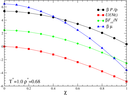
Figure 5: (Color online) Plot of the thermodynamic quantities $\beta P/\rho$, $U/N\epsilon$,$\beta F_{ex}/N$, $\beta\mu$ as a function of $\chi$ for $T^{*}=1.0$ and $\rho^{*}=0.68$ corresponding to a high density point in the gas phase, above the critical temperature.

As one might have predicted at the outset, as $\chi$ decreases all thermodynamic quantities display a tendency toward a decrease of the importance of attractions with respect to repulsions, that become the only interactions in the hard-sphere limit $\chi=0$. The internal energy $U/N\epsilon$, for instance, tends to increase from negative values and vanishes as the HS limit $\chi=0$ is reached. Similar features occur for the other thermodynamic variables.

In these results, we note that there is a monotonic dependence on the coverage $\chi$ of all thermodynamical quantities reported in Fig.5. This is due to the fact that, in their derivation, an orientational average is always present (see e.g. Eqs.(38) and (39)). This is however not mirrored by the $\chi$ dependence of the pair correlation functions $g(12)$ that, as remarked, keeps track of the detailed orientational dependence with respect to the relative angular position $\hat{\mathbf{r}}_{12}(\Omega)$ of the two particles, and with respect to the relative orientation of the two unit vectors $\hat{\mathbf{n}}_{1}(\omega)_{1}$ and $\hat{\mathbf{n}}_{2}(\omega_{2})$ associated with the patch orientations, in addition to the relative distance $r_{12}$.

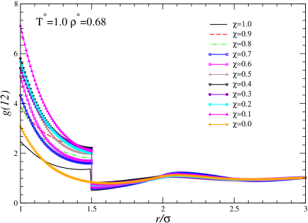
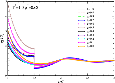
Figure 6: (Color online) Plot of the pair correlation function $g(12)$ as a function of $r$ for the same state point as before $T^{*}=1.0$ and $\rho^{*}=0.68$ and different coverages $\chi$. Top panel refers to the head-to-head configuration, bottom panel to the perpendicular counterpart (see Fig.4). Different curves are distinguished by the same sequences of symbols (and colors in the on-line version) in both cases.

This is shown in Fig.6 where the $g(12)$ is plotted as a function of $r\equiv r_{12}$ for different coverages, in the molecular frame where $\hat{\mathbf{r}}_{12}=\hat{\mathbf{z}}$. The head-to-head configuration (top panel) represents the case where the attractive patches are facing one another, that is $\hat{\mathbf{n}}_{2}\cdot\hat{\mathbf{n}}_{1}=1$, whereas the other interesting case (bottom panel) the patches are perpendicular one another, that is $\hat{\mathbf{n}}_{2}\cdot\hat{\mathbf{n}}_{1}=0$. In all cases, a herratic coverage dependence can be clearly observed. Consider for instance the head-to-head case (top panel). As $\chi$ is reduced from the isotropic SW value $\chi=1.0$ to $\chi=0.9$, the contact value at $r=\sigma^{+}$ increases, a clear indication of the increased probability for this configuration as compared, for instance, with the perpendicular configuration (bottom panel), where the contact value decreases. This is confirmed by a parallel increase in the discontinuity at $r=\lambda\sigma$ and mirrored by a corresponding reduction of the same discontinuity in the perpendicular configuration. As $\chi$ is further decreased to $\chi=0.8$, there is a clear reduction of the discontinuity at $r=\lambda\sigma$ accompained by only a negligible variation of the contact value, and there is no clear trend within the well width $\sigma<r<\lambda\sigma$ in both configurations, until the half coverage value ($\chi=0.5$) is reached. Interestingly, this value corresponds to the Janus limit of even philicities, and clearly plays a particular role, as already suggested by numerical simulations of the corresponding phase diagram (Sciortino et al 2009, 2010). For lower coverages, the contact values again increase for the head-to-head configurations, and decrease for the perpendicular configurations, indicating a marked tendency to form micelles, as already observed in numerical simulations. This region of the phase diagram is inherently interesting. As a matter of fact, at $\chi=0.5$ (Janus limit) numerical simulations show (Sciortino et al 2009) that, at sufficiently low temperatures and high densities, these double-face spheres tend spontaneously to aggregate into single or multiple layer clusters, to maximize all favourable contacts. These clusters have the attractive parts (that mimic the hydrophobic nature of the original experiments) buried inside and the hard-sphere parts externally exposed. Upon further cooling, this micellization tendency destabilizes more and more the liquid-gas transition that eventualy get almost completed inhibited (Sciortino et al 2009). This is a peculiar feature of the Janus case and it is not shared by any higher value of coverage that display a conventional gas-liquid transition, albeit with significantly reduced critical temperatures and densities. No simulations have been able so far to probe the region below the Janus limit (i.e. for $\chi<0.5$), due to the extremely low temperatures involved, but it is reasonable to expect again an absence of gas-liquid transition in view of the impossibility for the system to form clusters sufficiently large to yield a percolating network. This case strongly contrasts with the low $\chi$ counterpart of the two-patches case, where the attractive surface is spread on the two opposite poles of each sphere. In that case it has been shown (Giacometti et al 2010) that the value $\chi=0.5$ does not play any peculiar role, and the gas-liquid transition persists for coverages as low as $30\%$. Below that value the gas-liquid transition becomes metastable against crystalization, in very much the same way of what happens in the framework of spherical potentials of sufficiently short ranges.

Although the above pair correlations have been displayed in the molecular frame, where the $\hat{\mathbf{z}}$ axis is taken along the $\hat{\mathbf{r}}_{12}$ direction, integral equation theory is able to provide $g(12)$ in any arbitrary frame by performing an appropriate Clebsh-Gordan transformation (Gray and Gubbins 1984). This constitutes one of the two main advantages of this technique (the other being the limited computational cost) as compared to numerical simulations, where such details are virtually unaccessible. A simple way to obtain from $g(12)$ an isotropic quantity is to perform an angular integration over all three spherical angles $\omega_{1}$, $\omega_{2}$ and $\Omega_{12}$. The result is the projection along the spherical invariant with all three indices vanishing, that is $g_{000}(r)$ (Giacometti et al 2010). Likewise, the structure factor $S_{000}(k)$ can also be regarded as an isotropic angular average of anisotropic original dependence. This is also shown in Figure 7, where again the coverage dependence appears to be more regular, as discussed.

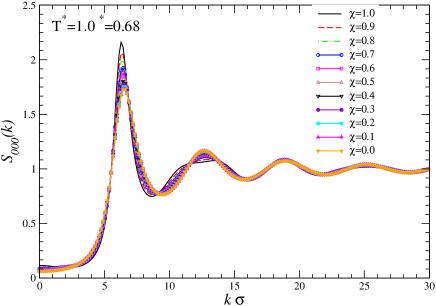
Figure 7: (Color online) Plot of the structure factor $S_{000}(k)$ for the Kern-Frenkel model as a function of $k\sigma$ for the same state point as before $T^{*}=1.0$ and $\rho^{*}=0.68$ and different coverages $\chi$. Different curves are distinguished by the same sequences of symbols (and colors in the on-line version) as in Fig.6.

IX Conclusions

In this paper we have reviewed some of the main difficulties encountered in the application of the OZ integral equation theory in the passage from simple to complex fluids. Two novel main features appear. On the one hand, colloidal suspensions are typically a multi-component system, and this requires the introduction of new techniques to cope with the difficulties arising with the mixture, some of which are an extension of those originally devised for ionic fluids. As a representative example, we have discussed the case of mixtures formed by species of different sizes and interacting via short-range attractive forces of the Baxter type, that combines the hard-sphere potential with an adhesive force acting only at contact. In the limit when the number of components of the mixture becomes very large, the distribution can be replaced by a continuous description (polydispersity), that is frequently represented by a Schultz distribution. We have assessed the effect of polydispersity on the structural and thermodynamical properties of the fluids, and how this can be accounted for in the framework of integral equation theory, both analytically and numerically. This is one of the fields where the work by Prof. Lesser Blum has made a remarkable impact.

We have additionally discussed how there exist a number of systems where surface inhomogeneities cannot be neglected, even to a first approximation. These include, globular proteins and – more recently – patchy colloids. In both cases, the potentials are no longer isotropic, and orientational effects play an important role. The implementation of integral equation calculations mirrors that devised for molecular fluids, with the important difference that the angular dependence typically displays step-wise discontinuities, mimicking either the presence of different surface groups in globular proteins, or different functionalities in patchy colloids. Two cases were discussed, as representative examples. In the Kern-Frenkel model, the potential is factorized into a part depending only on the distance and an angular part, tuning the interactions in the form of an on-off form. Depending on the form chosen for the radial dependence, the OZ integral equation theory can be tackled either analytically or purely numerically. We have discussed both cases and displayed representative examples of the results. In the first case, the radial dependence is again considered of the Baxter type, and this allows the use of the same approximations exploited in the isotropic counterpart, at the minimal cost of a slightly more complicate formalism. A major adantage of the integral equation theory is however displayed in the cases where numerical solutions are exploited with rather accurate closures, such as RHNC. Here, the numerical solution typically requires only few minutes of computational effort, as compared to several weeks of numerical simulations, and yet the obtained predictions are frequently rather accurate. Furthermore, the details of information that can be obtained from the analysis of pair correlation functions from integral equations is independent of the chosen frame and is unparalleled by any numerical simulations, where some form of orientational averages are always involved in order to have a reasonable statistics.

We believe that the potentialities of integral equation theory in complex fluids has still not be fully exploited so far, and that this methodology may become, in the next few years, the first and most reliable tool to tackle new challenging problems, before resorting to more computational demanding methods.

- (1) Baldini, G., Beretta S., Chirico G., Franz H., Maccioni E., Mariani P., and Spinozzi F., 1999. Salt induced association of -lactoglobulin studied by salt light and X-ray scattering. Macromolecules 32, 6128-6138.
- (2) R. J. Baxter, 1978. Percus-Yevick equation for hard spheres with surface adhesion. J Chem Phys 49, 2770-2774.
- (3) Blum L. 1975. Mean spherical model for asymmetric electrolytes. I. Method of solution. Mol Phys 30, 1529-1535.
- (4) Blum, L., and Høye J.S., 1978. Solution of the Ornstein-Zernike equation with Yukawa closure for a mixture. J. Stat. Phys. 19, 317-324.
- (5) Blum L., and Stell G., 1979. Polydisperse systems. I. Scattering function for polydisperse fluids of hard or permeable spheres. J Chem Phys 71, 42-46.
- (6) Carsughi F., Giacometti A., and Gazzillo D., 2000. Small Angle Scattering data analysis for dense polydisperse systems: the FLAC program. Computer Physics Communications 133, 66-75.
- (7) Ciccariello S., Gazzillo D., and Dejak C., 1982. ”Effective” dipolar forces in electrolytic solutions of structure-breaking salts. J Phys Chem 86, 2986-2994.
- (8) Ciccariello S., and Gazzillo D., 1982. A new form of the correction to the Coulombic contribution in the McMillan-Mayer ion-ion potential. Chem Phys Letts 93, 31-34.
- (9) Ciccariello S., and Gazzillo D., 1983. Thermodynamical behaviour and radial distribution functions of dilute systems of charged rigid spheres. Mol Phys 48, 1369-1381.
- (10) Ciccariello S., and Gazzillo D., 1985. A reasonable candidate for the McMillan-Mayer ion-ion potential of strong 1-1 electrolytes. J Chem Soc, Faraday Trans 2, 81, 1163-1177.
- (11) Debye, P., Hückel, E. 1923. Zur Theorie der Elektrolyten. I. Gefrierpunktserniedrigung und verwandte Erscheinungen (On the Theory of Electrolytes. I. Freezing Point Depression and Related Phenomena). Physicalische Zeit 24, 185-206.
- (12) El Mendoub E. B., Wax J. F., Charpentier I., and Jakse N.2008. Integral equation study of the square-well fluid for varying attraction range. Mol. Phys. 106, 2667–2675.
- (13) Fantoni R., Gazzillo D., and Giacometti A., 2005a. Stability boundaries, percolation threshold, and two-phase coexistence for polydisperse fluids of adhesive colloidal particles. J Chem Phys 122, 034901–1-15.
- (14) Fantoni R., Gazzillo D., and Giacometti A., 2005b. Thermodynamic instabilities of a binary mixture of sticky hard spheres. Phys Rev E 72, 011503–1-15.
- (15) Fantoni R., Gazzillo D., Giacometti A., and Sollich P., 2006. Phase behaviour of weakly polydisperse sticky hard spheres. Perturbation theory for the Percus-Yevick solution. J Chem Phys 125, 164504–1-16.
- (16) Fantoni R., Gazzillo D., Giacometti A., Miller M. A., and Pastore G. 2007. Patchy sticky hard spheres: Analytical study and Monte Carlo simulations. J. Chem. Phys. 127, 234507–1-16.
- (17) Gazzillo D., Giacometti A., and Carsughi F., 1997. Scattering functions for multicomponent mixtures of charged hard spheres, including the polydisperse limit. Analytic expressions in the Mean Spherical Approximation. J Chem Phys 107, 10141-10153.
- (18) Gazzillo D., Giacometti A., Della Valle R. G., Venuti E.; and Carsughi F., 1999a. A scaling approximation for structure factors in the integral equation theory of polydisperse nonionic colloidal fluids, J Chem Phys 111, 7636-7645.
- (19) Gazzillo D., Giacometti A., and Carsughi F., 1999b. Corresponding-states approach to small-angle scattering from polydisperse ionic colloidal fluids. Phys Rev E 60, 6722-6733.
- (20) Gazzillo D., and Giacometti A., 2000. Structure factors for the simplest solvable model of polydisperse colloidal fluids with surface adhesion. J Chem Phys 113, 9837-9848.
- (21) Gazzillo D., and Giacometti A., 2002. Polydisperse fluid mixtures of adhesive colloidal particles, Physica A 304, 202-210.
- (22) Gazzillo D., and Giacometti A., 2003. Pathologies in the sticky limit of hard sphere Yukawa models for colloidal fluids: a possible correction. Mol Phys 101, 2171-2179.
- (23) Gazzillo D., and Giacometti A., 2003. Structure factor for polydisperse fluids of particles with surface adhesion. J Appl Cryst 36, 832-835.
- (24) Gazzillo D., and Giacometti A., 2004. Analytic solutions for Baxter’s model of sticky hard sphere fluids within closures different from the Percus-Yevick approximation. J Chem Phys 120, 4742-4754.
- (25) Gazzillo D., Giacometti A., Fantoni R., and Sollich P., 2006. Multicomponent adhesive hard sphere models and short-ranged attractive interactions in colloidal or micellar solutions. Phys Rev E 74, 051407–1-14.
- (26) Gazzillo D., Giacometti A., and Fantoni R., 2006. Phase behaviour of polydisperse sticky-hard-sphere fluids: analytical solutions and perturbation theory. Mol Phys 104, 3451 – 3459.
- (27) Gazzillo D., Fantoni R., and Giacometti A. 2008. Fluids of spherical molecules with dipolarlike nonuniform adhesion: An analyitically solvable anisotropic model. Phys. Rev. E 78, 0212010-1–20.
- (28) Gazzillo D., Fantoni R., and Giacometti A. 2009. Local orientational ordering in fluids of spherical molecules with dipolarlike anisotropic adhesion. Phys. Rev. E 80, 061207-1–7.
- (29) Gazzillo D. 2010. Dipolar sticky hard spheres within the Percus-Yevick approximation plus orientational linearization. J. Chem. Phys. 133, 034511-1–13.
- (30) Gazzillo D. 2011. Fluids of hard spheres with dipolar-like patch interactions and effect of adding an isotropic adhesion, Mol. Phys. 109, 55-64.
- (31) Giacometti A., Gazzillo D., Pastore G., and Kanti Das T., 2005. Numerical study of a binary Yukawa model in regimes characteristic of globular proteins in solutions. Phys Rev E 71, 031108–1-10.
- (32) Giacometti A., Pastore G., and Lado F. 2009. Liquid-vapor coexistence in square-well fluids: a RHNC study. Mol. Phys. 107, 555–562.
- (33) Giacometti A., Lado F., Largo J., Pastore G., and Sciortino F. 2009. Phase diagram and structural properties for one-patch particles. J. Chem. Phys. 131 , 174114–1-14.
- (34) Giacometti A., Lado F., Largo J., Pastore G., and Sciortino F. 2010. Effect of patch size and number within a simple model of patchy particles. J. Chem. Phys. 132 , 174110–1-15.
- (35) Ginoza, M., 1990. Simple MSA solution and thermodynamic theory in a hard-sphere Yukawa system. Mol. Phys. 71,145-156.
- (36) Ginoza M., and Yasutomi M., 1997. Analytical model of the equation of state of the hard sphere Yukawa polydisperse fluid: interaction polydispersity effect. Mol Phys 91, 59-63.
- (37) Ginoza M., and Yasutomi M., 1998a. Analytical model of the static structure factor of a colloidal dispersion: interaction polydispersity effect. Mol Phys 93, 399-404.
- (38) Ginoza M., and Yasutomi M., 1998b. Analytical structure factors for colloidal fluids with size and interaction polydispersities. Phys Rev E 58, 3329-3333.
- (39) Ginoza M., and Yasutomi M., 1998c. Analytical model for the thermodynamic properties of a colloidal dispersion with size and ’charge’ polidispersities. Mol Phys 95, 163-167.
- (40) Gray C. G., and Gubbins K. E. 1984. Theory of molecular fluids, Vol. I (Clarendon Press, Oxford).
- (41) Hansen J.P., and McDonald I. R. 2006. Theory of Simple Liquids, 3rd Ed. (Academic Press, Amsterdam).
- (42) Hong L., Cacciuto A., Luijten E., and Granick S. 2008. Cluster of Amphiphilic Colloidal Spheres. Langmuir 24, 621–625.
- (43) Høye J. S., and Stell G., 1977. New self-consistent approximations for ionic and polar fluids, J. Chem. Phys. 67, 524-529
- (44) Jackson G., Chapman W.G., and Gubbins K.E. 1988. Phase equilibra of associating fluids: chain molecules with multiple bonding sites. Mol. Phys. 65, 1057–1079 (1988).
- (45) Kahl G., Schöll-Paschinger E., and Stell G., 2002. Phase Transition and critical behavior of simple fluids and their mixtures. J. of Phys.: Condens. Mat. 14, 9153-9169
- (46) Kern N., and Frenkel D., 2003. Fluid-fluid coexistence in colloidal systems with short-ranged strongly directional attractions. J. Chem. Phys. 118, 9882–9889.
- (47) Lado F. 1982. A local thermodynamic criterion for the Reference-Hypernetted Chain equation. Phys. Lett. A 89, 196–198.
- (48) Lado F. 1982. Integral equations for fluids of linear molecules. I. General formulation. Mol. Phys. 47, 283–298.
- (49) Lado F. 1982. Integral equations for fluids of linear molecules. II. Hard dumbell solution. Mol. Phys. 47, 299–312 299 (1982).
- (50) Morita T.1960. Theory of classical fluids: hyper-netted chain approximation III. Prog. Theor. Phys. 23, 829–845
- (51) Pawar A. B. and Kretzchmar I. 2010. Fabrication, Assembly, and Application of Patchy Particles. Macromol. Rapid Commun, 31, 150–168.
- (52) Pini D., Stell G., and Wilding N. B., 1998. A liquid-state theory that remains successful in the critical region. Mol. Phys.95, 483-494
- (53) Santos A., Fantoni R., and Giacometti A. 2009. Thermodynamic consistency of energy and virial routes: An exact proof within the linearized Debye-Hückel theory. J. Chem. Phys. 131, 181105–1-3.
- (54) Schöll-Paschinger E., Levesque D., Weiss J.J. and Kahl G., 2005. Phase diagram of a binary symmetric hard-core Yukawa mixtures, J. Chem. Phys. 122, 024507–1-7.
- (55) Sciortino F., Giacometti A., Pastore G. 2009. Phase diagram of Janus Particles. Phys. Rev. Lett. 103, 237801–1-4.
- (56) Sciortino F., Giacometti A., and Pastore G. 2010. A numerical study of one-patch colloidal particles: from square-well to Janus. Phys. Chem. Chem. Phys. 12, 11869–11877.
- (57) Spinozzi F., Gazzillo D., Giacometti A., Mariani P., and Carsughi F., 2002. Interaction of proteins in solution from small-angle scattering: a perturbative approach. Biophys J 82, 2165-2175.
- (58) Stell G. 1991. Sticky spheres and related systems. J. Stat. Phys. 63, 1203–1221.
- (59) Triolo R., Blum L., and Floriano M. A., 1977, Simple electrolytes in the Mean Spherical Approximation. III. A workable model for aqueous solutions. J Chem Phys 67, 5956-5959.
- (60) Triolo R, Blum L. and Floriano M.A., 1978. Simple electrolytes in the Mean Spherical Approximation. 2. Study of a refined model. J. Phys. Chem. 82, 1368-1370.
- (61) Vervey E. J., and Overbeek J. Th. G., 1948. Theory of the Stability of Lyophobic Colloids, (Elsevier, Amsterdam).
- (62) Vrij A., 1978. Light scattering of a concentrated multicomponent system of hard spheres in the Percus-Yevick approximation. J Chem Phys 69, 1742-1747.
- (63) Walther A. and Müller A. H. 2008. Janus particles. Soft Matter 4, 663–668.
- (64) White R. P. and Lipson J. E. G. 2007. Square-well mixtures: a study of their coexistence using theory and simulations. Mol. Phys. 105, 1983–1997.