Ergodic Mirror Descent

Abstract

We generalize stochastic subgradient descent methods to situations in which we do not receive independent samples from the distribution over which we optimize, instead receiving samples coupled over time. We show that as long as the source of randomness is suitably ergodic—it converges quickly enough to a stationary distribution—the method enjoys strong convergence guarantees, both in expectation and with high probability. This result has implications for stochastic optimization in high-dimensional spaces, peer-to-peer distributed optimization schemes, decision problems with dependent data, and stochastic optimization problems over combinatorial spaces.

1 Introduction

In this paper, we analyze a new algorithm, Ergodic Mirror Descent, for solving a class of stochastic optimization problems. We begin with a statement of the problem. Let $\{F(\cdot;\xi),\xi\in\Xi\}$ be a collection of closed convex functions whose domains contain the common closed convex set $\mathcal{X}\subseteq\mathbb{R}^{d}$. Let $\Pi$ be a probability distribution over the statistical sample space $\Xi$ and consider the convex function $f:\mathcal{X}\rightarrow\mathbb{R}$ defined by the expectation

$$f(x):=\mathbb{E}_{\Pi}[F(x;\xi)]=\int_{\Xi}F(x;\xi)d\Pi(\xi).$$ (1)

We study algorithms for solving the following problem:

$$\mathop{\rm minimize}_{x}~{}f(x)~{}~{}~{}\mbox{subject to}~{}~{}~{}x\in\mathcal{X}.$$ (2)

A wide variety of stochastic optimization methods for solving the problem (2) have been explored in an extensive literature [35, 32, 29, 22, 30]. We study procedures that do not assume it is possible to receive samples from the distribution $\Pi$, instead receiving samples $\xi$ from a stochastic process $P$ indexed by time $t$, where the stochastic process $P$ converges to the stationary distribution $\Pi$. This is a natural relaxation, because in many circumstances the distribution $\Pi$ is not even known—for example in statistical applications—and we cannot receive independent samples. In other scenarios, it may be hard to even draw samples from $\Pi$ efficiently, such as when $\Xi$ is a high-dimensional or combinatorial space, but it is possible [19] to design Markov chains that converge to the distribution $\Pi$. Further, in computational applications, it is often unrealistic to assume that one actually has access to a source of independent randomness, so studying the effect of correlation is natural and important [17].

Our approach to solving the problem (2) is related to classical stochastic gradient descent algorithms [35, 32], where one assumes access to samples $\xi$ from the distribution $\Pi$ and performs gradient updates using $\nabla F(x;\xi)$. When $\Pi$ is concentrated on a set of $n$ points and the functions $F$ are not necessarily differentiable, the incremental subgradient method of Nedić and Bertsekas [29] applies, and the objective is of the form $f(x)=\frac{1}{n}\sum_{i=1}^{n}f_{i}(x)$. More generally, our problem belongs to the family of stochastic problems with exogenous correlated noise [22] where the goal is to minimize $\mathbb{E}_{\Pi}[F(x;\xi)]$ as in the objective (2), but we have access only to samples $\xi$ that are not independent over time. Certainly a number of researchers in control, optimization, stochastic approximation, and statistics have studied settings where stochastic data is not i.i.d. (see, for example, the books [22, 38] and the numerous references therein). Nonetheless, classical results in this setting are asymptotic in nature and generally do not provide finite sample or high-probability convergence guarantees; our work provides such results.

Our method borrows from standard stochastic subgradient and stochastic mirror descent methodology [31, 30], but we generalize this work in that we receive samples not from the distribution $\Pi$ but from an ergodic process $\xi_{1},\xi_{2},\ldots$ converging to the stationary distribution $\Pi$. In spite of the new setting, we do not modify standard stochastic subgradient algorithms; our algorithm receives samples $\xi_{t}$ and takes mirror descent steps with respect to the subgradients of $F(x;\xi_{t})$. Consequently, our approach generalizes several recent works on stochastic and non-stochastic optimization, including the randomized incremental subgradient method [29] as well as the Markov incremental subgradient method [20, 34]. There are a number of applications of this work: in control problems, data is often coupled over time or may come from an autoregressive process [22]; in distributed sensor networks [23], a set of wireless sensors attempt to minimize an objective corresponding to a sequence of correlated measurements; and in statistical problems, data comes from an unknown distribution and may be dependent [42]. See our examples and experiments in § 4 and § 5, as well as the examples in the paper by Ram et al. [34], for other motivating applications.

The main result of this paper is that performing stochastic gradient or mirror descent steps as described in the previous paragraph is a provably convergent optimization procedure. The convergence is governed by problem-dependent quantities (namely the radius of $\mathcal{X}$ and the Lipschitz constant of the functions $F$) familiar from previous results on stochastic methods [29, 43, 30] and also depends on the rate at which the stochastic process $\xi_{1},\xi_{2},\ldots$ converges to its stationary distribution. Our three main convergence theorems characterize the convergence rate of Ergodic Mirror Descent in terms of the mixing time $\tau_{\rm mix}$ (the time it takes the process $\xi_{t}$ to converge to the stationary distribution $\Pi$, in a sense we make precise later) in expectation, with high probability, and when the mixing times of the process are themselves random. In particular, we show that this rate is $\mathcal{O}\left(\sqrt{\frac{\tau_{\rm mix}}{T}}\right)$ for a large class of ergodic processes, both in expectation and with high probability. We also give a lower bound that shows that our results are tight: they cannot (in general) be improved by more than numerical constants.

The remainder of the paper is organized as follows. Section 2 contains our main assumptions and a description of the algorithm. Following that, we collect our main technical results in § 3. We expand on these results in example corollaries throughout § 4 and give numerical simulations exploring our algorithms in § 5. We provide complete proofs of all our results in § 6 and the appendices.

Notation

For the reader’s convenience, we collect our (standard) notation here. A function $f$ is $G$-Lipschitz with respect to a norm $\left\|\cdot\right\|$ if $|f(x)-f(y)|\leq G\left\|x-y\right\|$. The dual norm $\left\|\cdot\right\|_{*}$ to a norm $\left\|\cdot\right\|$ is defined by $\left\|z\right\|_{*}:=\sup_{\left\|x\right\|\leq 1}\left\langle z,x\right\rangle$. A function $\psi$ is strongly convex with respect to the norm $\left\|\cdot\right\|$ over the domain $\mathcal{X}$ if

$$\psi(y)\geq\psi(x)+\left\langle\nabla\psi(x),y-x\right\rangle+\frac{1}{2}\left\|x-y\right\|^{2}~{}~{}\mbox{for}~{}x,y\in\mathcal{X}.$$

For a convex function $f$, we let $\partial f(x)=\{g\in\mathbb{R}^{d}\mid f(y)\geq f(x)+\left\langle g,y-x\right\rangle\}$ denote its subdifferential. For a matrix $A\in\mathbb{R}^{n\times m}$, we let $\rho_{i}(A)$ denote its $i$th largest singular value, and when $A\in\mathbb{R}^{n\times n}$ is symmetric we let $\lambda_{i}(A)$ denote its $i$th largest eigenvalue. The all-ones vector is $1\!\!1$, and we denote the transpose of the matrix $A$ by $A^{\top}$. We let $[n]$ denote the set $\{1,\ldots,n\}$. For functions $f$ and $g$, we write $f(n)=\mathcal{O}(g(n))$ if there exist $N<\infty$ and $C<\infty$ such that $f(n)\leq Cg(n)$ for $n\geq N$, and $f(n)=\Omega(g(n))$ if there exist $N<\infty$ and $c>0$ such that $f(n)\geq cg(n)$ for $n\geq N$. For a probability measure $P$ and measurable set or event $A$, $P(A)$ denotes the mass $P$ assigns $A$.

2 Assumptions and algorithm

We now turn to describing our algorithm and the assumptions underlying it. We begin with a description of the algorithm, which is familiar from the literature on mirror descent algorithms [31, 3]. Specifically, we generalize the stochastic mirror descent algorithm [31, 30], which in turn generalizes gradient descent to elegantly address non-Euclidean geometry. The algorithm is based on a prox-function $\psi$, a differentiable convex function defined on $\mathcal{X}$ assumed (w.l.o.g. by scaling) to be $1$-strongly convex with respect to the norm $\left\|\cdot\right\|$ over $\mathcal{X}$. The Bregman divergence $D_{\psi}$ generated by $\psi$ is defined as

$$D_{\psi}(x,y):=\psi(x)-\psi(y)-\left\langle\nabla\psi(y),x-y\right\rangle\geq\frac{1}{2}\left\|x-y\right\|^{2}.$$ (3)

We assume $\mathcal{X}$ is compact and that there exists a radius $R<\infty$ such that

$$D_{\psi}(x,y)\leq\frac{1}{2}R^{2}~{}~{}~{}\mbox{for}~{}x,y\in\mathcal{X}.$$ (4)

The Ergodic Mirror Descent (EMD) algorithm is an iterative algorithm that maintains a parameter $x(t)\in\mathcal{X}$, which it updates using stochastic gradient information to form $x(t+1)$. Specifically, let $P^{t}$ denote the distribution of the stochastic process $P$ at time $t$. We assume that we receive a sample $\xi_{t}\sim P^{t}$ at each time step $t$. Given $\xi_{t}$, EMD computes the update

$$g(t)\in\partial F(x(t);\xi_{t}),~{}~{}~{}x(t+1)=\mathop{\rm argmin}_{x\in\mathcal{X}}\left\{\left\langle g(t),x\right\rangle+\frac{1}{\alpha(t)}D_{\psi}(x,x(t))\right\}.$$ (5)

The initial point $x(1)$ may be selected arbitrarily in $\mathcal{X}$, and here $\alpha(t)$ is a non-increasing (time-dependent) stepsize. The algorithm (5) reduces to projected gradient descent with the choice $\psi(x)=\frac{1}{2}\left\|{x}\right\|_{2}^{2}$, since then $D_{\psi}(x,y)=\frac{1}{2}\left\|{x-y}\right\|_{2}^{2}$.

Our main assumption on the functions $F(\cdot;\xi)$ regards their continuity and subdifferentiability properties, though we require a bit more notation. Let $\mathsf{G}(x;\xi)\in\partial F(x;\xi)$ denote a fixed and measurable element of the subgradient of $F(\cdot;\xi)$ evaluated at the point $x$, where (without loss of generality) we assume that in the EMD algorithm (5) we have $g(t)=\mathsf{G}(x(t);\xi_{t})$. We let $\mathcal{F}_{t}$ denote the $\sigma$-field of the first $t$ random samples $\xi_{1},\ldots,\xi_{t}$ from the stochastic process $P$ (that is, $\xi_{t}$ is drawn according to $P^{t}$). We make one of the following two assumptions, where in each the norm $\left\|\cdot\right\|$ is the norm with respect to which $\psi$ is strongly convex (3):

Assumption A (Finite single-step variance).

Let $x$ be measurable with respect to the $\sigma$-field $\mathcal{F}_{t-1}$. There exists a constant $G<\infty$ such that with probability 1

$$\mathbb{E}[\left\|\mathsf{G}(x;\xi_{t})\right\|_{*}^{2}\mid\mathcal{F}_{t-1}]\leq G^{2}.$$

Assumption B.

For $\Pi$-almost every $\xi$, the functions $F(\cdot;\xi)$ are $G$-Lipschitz continuous functions with respect to a norm $\left\|\cdot\right\|$ over $\mathcal{X}$. That is,

$$|F(x;\xi)-F(y;\xi)|\leq G\left\|x-y\right\|~{}~{}~{}\mbox{for~{}}x,y\in\mathcal{X}.$$

As a consequence of Assumption B, for any $g\in\partial F(x;\xi)$ we have that $\left\|g\right\|_{*}\leq G$ (e.g., [16]), and it is clear that the expected function $f$ is also $G$-Lipschitz. Assumption B implies Assumption A, though Assumption A still guarantees $f$ is $G$-Lipschitz, and under either assumption, we have

$$\mathbb{E}\left[\left\|\mathsf{G}(x;\xi)\right\|_{*}^{2}\right]=\mathbb{E}\left[\mathbb{E}\left[\left\|\mathsf{G}(x;\xi)\right\|_{*}^{2}\mid\mathcal{F}_{t-1}\right]\right]\leq G^{2}.$$ (6)

Having described the family of functions $\{F(\cdot;\xi):\xi\in\Xi\}$, we recall a few definitions from probability theory that are essential to the presentation of our results. We measure the convergence of the stochastic process $P$ using one of two common statistical distances [13]: the Hellinger distance and the total variation distance (our definitions are a factor of 2 different from some definitions of these metrics). The total variation distance between probability distributions $P$ and $Q$ defined on a set $\Xi$, assumed to have densities $p$ and $q$ with respect to an underlying measure $\mu$, is

$$d_{{}_{\rm TV}}(P,Q):=\int_{\Xi}|p(\xi)-q(\xi)|d\mu(\xi)=2\sup_{A\subset\Xi}|P(A)-Q(A)|,$$ (7)

the supremum taken over measurable subsets of $\Xi$. The squared Hellinger distance is

$$d_{\rm hel}(P,Q)^{2}=\int_{\Xi}\left(\sqrt{\frac{p(\xi)}{q(\xi)}}-1\right)^{2}q(\xi)d\mu(\xi)=\int_{\Xi}\left(\sqrt{p(\xi)}-\sqrt{q(\xi)}\right)^{2}d\mu(\xi).$$ (8)

It is a well-known fact [13] that for any probability distributions $P$ and $Q$,

$$d_{\rm hel}(P,Q)^{2}\leq d_{{}_{\rm TV}}(P,Q)\leq 2d_{\rm hel}(P,Q).$$ (9)

Using the total variation (7) and Hellinger (8) metrics, we now describe our notion of mixing (convergence) of the stochastic process $P$. Recall our definition of the $\sigma$-field $\mathcal{F}_{t}=\sigma(\xi_{1},\ldots,\xi_{t})$. Let $P^{t}_{[s]}$ denote the distribution of $\xi_{t}$ conditioned on $\mathcal{F}_{s}$ (i.e. given the initial samples $\xi_{1},\ldots,\xi_{s}$), so for measurable $A\subset\Xi$ we have $P^{t}_{[s]}(A):=P(\xi_{t}\in A\mid\mathcal{F}_{s})$. We measure convergence of $P$ to $\Pi$ in terms of the mixing time of the different $P^{t}_{[s]}$, defined for the Hellinger and total variation distances as follows. In the definitions, let $p^{t}_{[s]}$ and $\pi$ denote the densities of $P^{t}_{[s]}$ and $\Pi$, respectively.

Definition 1.

The total variation mixing time $\tau_{{}_{\rm TV}}(P_{[s]},\epsilon)$ of the sampling distribution $P$ conditioned on the $\sigma$-field of the initial $s$ samples $\mathcal{F}_{s}=\sigma(\xi_{1},\ldots,\xi_{s})$ is the smallest $t\in\mathbb{N}$ such that $d_{{}_{\rm TV}}(P_{[s]}^{s+t},\Pi)\leq\epsilon$,

$$\tau_{{}_{\rm TV}}(P_{[s]},\epsilon):=\inf\left\{t-s:t\in\mathbb{N},~{}\int_{\Xi}\left|p_{[s]}^{t}(\xi)-\pi(\xi)\right|d\mu(\xi)\leq\epsilon\right\}.$$

The Hellinger mixing time $\tau_{\rm hel}(P_{[s]},\epsilon)$ is the smallest $t$ such that $d_{\rm hel}(P_{[s]}^{s+t},\Pi)\leq\epsilon$,

$$\tau_{\rm hel}(P_{[s]},\epsilon):=\inf\left\{t-s:t\in\mathbb{N},~{}\int_{\Xi}\left(\sqrt{p_{[s]}^{t}(\xi)}-\sqrt{\pi(\xi)}\right)^{2}d\mu(\xi)\leq\epsilon^{2}\right\}.$$

Put another way, the mixing times $\tau_{{}_{\rm TV}}(P_{[s]},\epsilon)$ and $\tau_{\rm hel}(P_{[s]},\epsilon)$ are the number of additional steps required until the distribution of $\xi_{t}$ is close to the stationary distribution $\Pi$ given the initial $s$ samples $\xi_{1},\ldots,\xi_{s}$.

The following assumption, which makes the mixing times of the stochastic process $P$ uniform, is our main probabilistic assumption.

Assumption C.

The mixing times of the stochastic process $\{\xi_{i}\}$ are uniform in the sense that there exist uniform mixing times $\tau_{{}_{\rm TV}}(P,\epsilon),\tau_{\rm hel}(P,\epsilon)<\infty$ such that with probability $1$,

$$\tau_{{}_{\rm TV}}(P,\epsilon)\geq\tau_{{}_{\rm TV}}(P_{[s]},\epsilon)~{}~{}~{}\mbox{and}~{}~{}~{}\tau_{\rm hel}(P,\epsilon)\geq\tau_{\rm hel}(P_{[s]},\epsilon)$$

for all $\epsilon>0$ and $s\in\mathbb{N}$.

Assumption C is a weaker version of the common assumption of $\phi$-mixing in the probability literature (e.g. [9]); $\phi$-mixing requires convergence of the process over the entire “future” $\sigma$-field $\sigma(\xi_{t},\xi_{t+1},\ldots)$ of the process $\xi_{t}$. Any finite state-space time-homeogeneous Markov chain satisfies the above assumption, as do uniformly ergodic Markov chains on general state spaces [27].

We remark that the definition 1 of mixing time does not assume that the distributions $P_{[s]}$ are time-homogeneous. Indeed, Assumption C requires only that there exists a uniform upper bound on the mixing times. We can weaken Assumption C to allow randomness in the probability distributions $P^{t}_{[s]}$ themselves, that is, conditional on $\mathcal{F}_{s}$, the mxing time $\tau_{{}_{\rm TV}}(P_{[s]},\epsilon)$ is an $\mathcal{F}_{s}$-measurable random variable. Our weakened probabilistic assumption is

Assumption D.

The mixing times of the stochastic process $\{\xi_{i}\}$ are stochastically uniform in the sense that there exists a uniform mixing time $\tau_{{}_{\rm TV}}(P,\epsilon)<\infty$, continuous from the right as a function of $\epsilon$, such that for all $\epsilon>0$, $s\in\mathbb{N}$, and $c\in\mathbb{R}$

$$P\!\left(\tau_{{}_{\rm TV}}(P_{[s]},\epsilon)\geq\tau_{{}_{\rm TV}}(P,\epsilon)+\kappa c\right)\leq\exp(-c).$$

Assumption D allows us to provide convergence guarantees for a much wider range of processes, such as auto-regressive processes, than permitted by Assumption C.

3 Main results

With our assumptions in place, we can now give our main results. We begin with three general theorems that guarantee the convergence of the EMD algorithm in expectation and with high probability. The second part of the section shows that our analysis is sharp—unimprovable by more than numerical constant factors—by giving an information-theoretic lower bound on the convergence rate of any optimization procedure receiving non-i.i.d. samples from $P$.

3.1 Convergence guarantees

Our first result gives convergence in expectation of the EMD algorithm (5); we provide the proof in § 6.2.

Theorem 1.

Let Assumption C hold and let $x(t)$ be defined by the EMD update (5) with non-increasing stepsize sequence $\{\alpha(t)\}$. Let $x^{\star}\in\mathcal{X}$ be arbitrary and let (4) hold. If Assumption A holds, then for any $\epsilon>0$,

$$\mathbb{E}\bigg{[}\sum_{t=1}^{T}\left(f(x(t))-f(x^{\star})\right)\bigg{]}$$

$$\quad\leq\frac{R^{2}}{2\alpha(T)}+\frac{G^{2}}{2}\sum_{t=1}^{T}\alpha(t)+3T\epsilon GR+(\tau_{\rm hel}(P,\epsilon)-1)\bigg{[}G^{2}\sum_{t=1}^{T}\alpha(t)+RG\bigg{]},$$

while if Assumption B holds, then for any $\epsilon>0$,

$$\mathbb{E}\bigg{[}\sum_{t=1}^{T}\left(f(x(t))-f(x^{\star})\right)\bigg{]}$$

$$\quad\leq\frac{R^{2}}{2\alpha(T)}+\frac{G^{2}}{2}\sum_{t=1}^{T}\alpha(t)+T\epsilon GR+(\tau_{{}_{\rm TV}}(P,\epsilon)-1)\bigg{[}G^{2}\sum_{t=1}^{T}\alpha(t)+RG\bigg{]}.$$

The expectation in both bounds is taken with respect to the samples $\xi_{1},\ldots,\xi_{T}$.

We obtain an immediate corollary to Theorem 1 by applying Jensen’s inequality to the convex function $f$:

Corollary 1.

Define $\widehat{x}(T)=\frac{1}{T}\sum_{t=1}^{T}x(t)$ and let the conditions of Theorem 1 hold. If Assumption A holds, then for any $\epsilon>0$

$$\mathbb{E}[f(\widehat{x}(T))-f(x^{\star})]\leq\frac{R^{2}}{2\alpha(T)T}+\frac{G^{2}}{2T}\sum_{t=1}^{T}\alpha(t)+3\epsilon GR+\frac{\tau_{\rm hel}(P,\epsilon)-1}{T}\bigg{[}G^{2}\sum_{t=1}^{T}\alpha(t)+RG\bigg{]}.$$

If Assumption B holds, then for any $\epsilon>0$

$$\mathbb{E}[f(\widehat{x}(T))-f(x^{\star})]\leq\frac{R^{2}}{2\alpha(T)T}+\frac{G^{2}}{2T}\sum_{t=1}^{T}\alpha(t)+\epsilon GR+\frac{\tau_{{}_{\rm TV}}(P,\epsilon)-1}{T}\bigg{[}G^{2}\sum_{t=1}^{T}\alpha(t)+RG\bigg{]}.$$

Corollary 1 shows that so long as the stepsize sequence $\alpha(t)$ is non-increasing and satisfies the asymptotic conditions $T\alpha(T)\rightarrow\infty$ and $(1/T)\sum_{t=1}^{T}\alpha(t)\rightarrow 0$, the EMD method converges. We can also provide similar high-probability convergence guarantees:

Theorem 2.

Let the conditions of Theorem 1 and Assumption B hold. Let $\delta\in(0,1)$ and define the average $\widehat{x}(T)=\frac{1}{T}\sum_{t=1}^{T}x(t)$. With probability at least $1-\delta$, for $\epsilon>0$ such that $\tau_{{}_{\rm TV}}(P,\epsilon)\leq T/2$,

$$f(\widehat{x}(T))-f(x^{\star}) \leq\frac{R^{2}}{2T\alpha(T)}+\frac{G^{2}}{2T}\sum_{t=1}^{T}\alpha(t)+\frac{\tau_{{}_{\rm TV}}(P,\epsilon)-1}{T}\bigg{[}G^{2}\sum_{t=1}^{T}\alpha(t)+GR\bigg{]}$$

$$\qquad\quad~{}+\epsilon GR+4GR\sqrt{\frac{\tau_{{}_{\rm TV}}(P,\epsilon)\log\frac{\tau_{{}_{\rm TV}}(P,\epsilon)}{\delta}}{T}}.$$

We provide the proof of this theorem in § 6.3. Note that the rate of convergence in Theorem 2 is identical to that obtained in Theorem 1 plus an additional term that arises as a result of the control of the deviation of the ergodic process around its expectation. The additional $\log\frac{1}{\delta}$-dependent term arises from the application of martingale concentration inequalities [2], which requires some care because the process $\{\xi_{t}\}$ is coupled over time. Nonetheless, as we discuss briefly following Corollary 2—and as made clear by our lower bound in Theorem 4—the additional terms introduce a factor of at most $\sqrt{\log\tau_{{}_{\rm TV}}(P,\epsilon)}$ to the bounds. That is, the dominant terms in the convergence rates (modulo logarithmic factors) also appear in the expected bounds in Theorem 1.

The last of our convergence theorems extends the previous two to the case when the stochastic process is not uniformly mixing, but has mixing properties that may depend on its state. We provide the proof of Theorem 3 in § 6.4.

Theorem 3.

Let the conditions of Theorem 2 hold, except that we replace the uniform mixing assumption C with the probabilistic mixing assumption D. Let $\delta\in(0,1)$. In the notation of Assumption D, define

$$\tau(\epsilon,\delta):=\tau_{{}_{\rm TV}}(P,\epsilon)+\kappa\left(\log\frac{2}{\delta}+2\log(T)\right).$$

With probability at least $1-\delta$, for any $x^{\star}\in\mathcal{X}$,

$$f(\widehat{x}(T))-f(x^{\star}) \leq\inf_{\epsilon>0}\bigg{\{}\frac{R^{2}}{2T\alpha(T)}+\frac{G^{2}}{2T}\sum_{t=1}^{T}\alpha(t)+\frac{\tau(\epsilon,\delta)-1}{T}\bigg{[}G^{2}\sum_{t=1}^{T}\alpha(t)+GR\bigg{]}$$

$$\qquad\qquad~{}+\epsilon GR+4GR\sqrt{\frac{\tau(\epsilon,\delta)\log\frac{\tau(\epsilon,\delta)}{\delta}}{T}}\,\bigg{\}}.$$

In § 4.3 we give two applications of Theorem 3 (to estimation in autoregressive processes and a fault-tolerant distributed optimization scheme) that show how it makes the applicability of our development substantially broader.

We now turn to a slight specialization of our bounds to build intuition and attain a simplified statement of convergence rates. Theorems 1, 2, and 3 hold for essentially any ergodic process that converges to the stationary distribution $\Pi$. For a large class of processes, the convergence of the distributions $P^{t}$ to the stationary distribution $\Pi$ is uniform and at a geometric rate [27]: there exist constants $\kappa_{1}$ and $\kappa_{2}$ such that $\tau_{{}_{\rm TV}}(P,\epsilon)\leq\kappa_{1}\log(\kappa_{2}/\epsilon)$. We have the following corollary for this special case; we only present the version yielding expected convergence rates, as the high-probability corollary is similar. In addition, by the fact (9) relating $d_{\rm hel}$ to $d_{{}_{\rm TV}}$, if the process $P$ satisfies $\tau_{{}_{\rm TV}}(P,\epsilon)\leq\kappa_{1}\log(\kappa_{2}/\epsilon)$, then there exist constants $\kappa_{1}^{\prime}$ and $\kappa_{2}^{\prime}$ such that $\tau_{\rm hel}(P,\epsilon)\leq\kappa_{1}^{\prime}\log(\kappa_{2}^{\prime}/\epsilon)$. Thus we only state the corollary for total variation mixing and under Assumption B; an analogous result holds under Assumption A for mixing with respect to the Hellinger distance.

Corollary 2.

Under the conditions of Theorem 1, assume in addition that $\tau_{{}_{\rm TV}}(P,\epsilon)\leq\kappa_{1}\log(\kappa_{2}/\epsilon)$ and let Assumption B hold. The EMD update (5) with stepsize $\alpha(t)=\alpha/\sqrt{t}$ satisfies

$$\mathbb{E}\left[f(\widehat{x}(T))-f(x^{\star})\right]\leq\frac{R^{2}}{2\alpha\sqrt{T}}+\frac{2\alpha G^{2}}{\sqrt{T}}\Big{(}\kappa_{1}\log\frac{\kappa_{2}}{\epsilon}\Big{)}+\epsilon GR+\frac{RG\kappa_{1}\log\frac{\kappa_{2}}{\epsilon}}{T}.$$

Proof    Using the definition $\alpha(t)=\alpha/\sqrt{t}$ and the integral bound

$$\sum_{t=1}^{T}\frac{1}{\sqrt{t}}\leq 1+\int_{1}^{T}t^{-1/2}dt=2\sqrt{T}-1<2\sqrt{T},$$ (10)

we have $\sum_{t=1}^{T}\alpha(t)\leq 2\alpha\sqrt{T}$. The corollary now follows from Theorem 1. ∎

We can obtain a simplified convergence rate with appropriate choice of the stepsize multiplier $\alpha$ and mixing parameter $\epsilon$: choosing $\alpha=R/(G\sqrt{\kappa_{1}\log(\kappa_{2}T)})$ and $\epsilon=T^{-1/2}$ reduces the corollary to

$$\mathbb{E}[f(\widehat{x}(T))-f(x^{\star})]=\mathcal{O}\left(\frac{RG\sqrt{\kappa_{1}\log(\kappa_{2}T)}}{\sqrt{T}}\right).$$ (11)

More generally, using the stepsize $\alpha(t)=\alpha/\sqrt{t}$ and the same argument as in Corollary 2 gives

$$\mathbb{E}[f(\widehat{x}(T))-f(x^{\star})]\leq\inf_{\epsilon>0}\left\{\frac{R^{2}}{2\alpha\sqrt{T}}+\frac{2\alpha G^{2}}{\sqrt{T}}\tau_{{}_{\rm TV}}(P,\epsilon)+\epsilon GR+\frac{RG(\tau_{{}_{\rm TV}}(P,\epsilon)-1)}{T}\right\}.$$ (12)

Again choosing $\epsilon=T^{-1/2}$ and defining the shorthand $\tau_{\rm mix}=\tau_{{}_{\rm TV}}(P,T^{-1/2})$, by choosing $\alpha=R/(G\sqrt{\tau_{\rm mix}})$, we see the bound (12) implies that

$$\mathbb{E}[f(\widehat{x}(T))-f(x^{\star})]\leq\frac{5RG}{2}\cdot\frac{\sqrt{\tau_{\rm mix}}}{\sqrt{T}}+\frac{RG}{\sqrt{T}}+\frac{RG(\tau_{\rm mix}-1)}{T}.$$ (13)

In the classical setting [30] of i.i.d. samples $\xi\sim\Pi$, stochastic gradient descent and its mirror descent generalizations attain convergence rates of $\mathcal{O}(RG/\sqrt{T})$. Since $\tau_{{}_{\rm TV}}(P,0)=\tau_{\rm hel}(P,0)=1$ for an i.i.d. process, the rate (12) shows that our results subsume existing results for i.i.d. noise. Moreover, they are sharp in the i.i.d. case, that is, unimprovable by more than a numerical constant factor [31, 1].

In addition, we note that the conclusions of Corollary 2 (and the bound (12)) hold—modulo an additional $\log\tau_{{}_{\rm TV}}(P,\epsilon)$—with high probability. We may also note that replacing $\epsilon GR$ with $3\epsilon GR$ and $\tau_{{}_{\rm TV}}$ with $\tau_{\rm hel}$ in the bound (12) yields a guarantee under Assumption A. Further, the step-size choice $\alpha(t)=\alpha/\sqrt{t}$ is robust—in a way similarly noted by Nemirovski et al. [30]—for quickly mixing ergodic processes. Indeed, using the inequalities (12) and (13), we see that setting the multiplier $\alpha=\gamma R/(G\sqrt{\tau_{\rm mix}})$ yields $\mathbb{E}[f(\widehat{x}(T))-f(x^{*})]=\mathcal{O}(\max\{\gamma,\gamma^{-1}\}RG\sqrt{\tau_{\rm mix}}/\sqrt{T})$, so mis-specification of $\alpha$ by a constant $\gamma$ leads to a penalty in convergence that scales at worst linearly in $\max\{\gamma^{-1},\gamma\}$. In classical stochastic approximation settings [35, 38, 22], one usually chooses step size sequence $\alpha(t)=\mathcal{O}(t^{-m})$ for $m\in\left({.5},{1}\right]$; in our case, such choices may yield sub-optimal rates because we study convergence of the averaged parameter $\widehat{x}(T)$ rather than the final parameter $x(t)$. Nonetheless, averaging is known to yield robustness in i.i.d. settings [32, 30], and moreover gives unimprovable convergence rates in many cases (see § 3.2 as well as references [31, 1]). We provide some evidence of this robustness in numerical simulations in § 5, and we see generally that EMD has qualitative convergence behavior similar to stochastic mirror descent for a broad class of ergodic processes.

Before continuing, we make two final remarks. First, none of our main theorems assume Markovianity or even homogeneity of the stochastic process $P$; all that is needed is that the mixing time $\tau_{{}_{\rm TV}}$ (or $\tau_{\rm hel}$) exists, or even that it exists only with some reasonably high probability. Previous work similar to ours [34, 20] assumes Markovianity (see also our discussion concluding § 4.3). Further, general ergodic processes do not always enjoy the geometric mixing assumed in Corollary 2, satisfying either Assumption D’s probabilistic mixing condition or simply mixing more slowly. In § 4.3, we present examples of such probabilistically mixing processes on general state spaces, while the bound (12) suggests an approach to attain convergence for more slowly mixing processes (see § 4.4).

3.2 Lower bounds and optimality guarantees

Our final main result concerns the optimality of the results we have presented. Informally, the theorem states that our results are unimprovable by more than numerical constant factors, though making this formal requires additional notation. In the stochastic gradient oracle model of convex optimization [31, 1], a method $\mathcal{M}$ issues queries of the form $x\in\mathcal{X}$ to an oracle that returns noisy function and gradient information. In our setting, the oracle is represented by the pair $\theta=(P,\mathsf{G})$, and when the oracle is queried at a point $x$ at time $t$ (i.e., this is the $t$th query $\theta$ has received), it draws a sample $\xi_{t}$ according to the distribution $P(\cdot\mid\xi_{1},\ldots,\xi_{t-1})$ and returns $\mathsf{G}(x,\xi_{t})\in\mathbb{R}^{d}$. The method issues a sequence of queries $x(1),\ldots,x(t)$ to the oracle and may use $\{\mathsf{G}(x(1),\xi_{1}),\ldots,\mathsf{G}(x(t),\xi_{t})\}$ to devise a new query point $x(t+1)$. For an oracle $\theta$, we define the error of the method $\mathcal{M}$ on a function $f$ after $T$ queries of the oracle as

$$\epsilon_{T}(\mathcal{M},f,\mathcal{X},\theta)=f(\widehat{x})-\inf_{x\in\mathcal{X}}f(x),$$ (14)

where $\widehat{x}$ denotes the method $\mathcal{M}$’s estimate of the minimizer of $f$ after seeing the $T$ samples $\{\mathsf{G}(x(1),\xi_{1}),\ldots,\mathsf{G}(x(T),\xi_{T})\}$. The quantity (14) is random, so we measure accuracy in terms of the expected value $\mathbb{E}_{\theta}[\epsilon_{T}(\mathcal{M},f,\mathcal{X},\theta)]$, where the expectation is taken with respect to the randomness in $\theta$.

Now we define a natural collection of stochastic oracles for our dependent setting.

Definition 2.

For $f$ convex, $\tau\in\mathbb{N}$, $G\in(0,\infty)$, and $p\in[1,\infty]$, the admissible oracle set $\Theta\left({f,\tau,G,p}\right)$ is the set of oracles $\theta=(P,\mathsf{G})$ for which there exists a probability distribution $\Pi$ on $\xi$ such that

$$\left\|\mathsf{G}(x;\xi)\right\|_{p}\leq G~{}\mbox{for~{}}x\in\mathcal{X}~{}\mbox{and}~{}\xi\in\Xi,~{}~{}~{}\mathbb{E}_{\Pi}[\mathsf{G}(x;\xi)]\in\partial f(x)~{}\mbox{for~{}}x\in\mathcal{X},$$

$$~{}~{}~{}\mbox{and}~{}~{}d_{{}_{\rm TV}}\left(P_{[t]}^{t+\tau},\Pi\right)=0~{}\mbox{for~{}all~{}}t\in\mathbb{N}~{}\mbox{with~{}probability~{}}1.$$

The set $\Theta\left({f,\tau,G,p}\right)$ is the collection of oracles $\theta=(P,\mathsf{G})$ for which the distribution $P$ has stationary distribution $\Pi$, mixing time bounded by $\tau$, and returns $\ell_{p}$-norm bounded stochastic subgradients of the function $f$. The condition $\left\|\mathsf{G}(x;\xi)\right\|_{p}\leq G$ guarantees that Assumptions A and B hold, while $d_{{}_{\rm TV}}(P_{[t]}^{t+\tau},\Pi)=0$ satisfies Assumption C. With Definition 2, for any collection $\mathcal{C}$ of convex functions $f$, we can define the minimax error over distributions with mixing times bounded by $\tau$ as

$$\epsilon_{T}^{*}(\mathcal{C},\mathcal{X},\tau,G,p):=\inf_{\mathcal{M}}~{}\sup_{f\in\mathcal{C}}\sup_{\theta\in\Theta\left({f,\tau,G,p}\right)}\mathbb{E}_{\theta}\left[\epsilon_{T}(\mathcal{M},f,\mathcal{X},\theta)\right].$$ (15)

We have the following theorem on this minimax error (see § 6.5 for a proof).

Theorem 4.

Let $\mathcal{X}\subseteq\mathbb{R}^{d}$ be a convex set containing the $\ell_{\infty}$ ball of radius $r$ for some $r>0$. Let $1/p+1/q=1$ and $p\geq 1$ and let the set $\mathcal{C}$ consist of convex functions that are $G$-Lipschitz continuous with respect to the $\ell_{q}$-norm over the set $\mathcal{X}$. For $p\in[1,2]$ and for any $\tau\in\mathbb{N}$, the minimax oracle complexity (15) satisfies

$$\epsilon_{T}^{*}(\mathcal{C},\mathcal{X},\tau,G,p)=\Omega\left(Gr\sqrt{d}\sqrt{\frac{\tau}{T}}\right).$$ (16a)

For $$p\in[2,\infty] \tau\in\mathbb{N}$$ and for any , the minimax oracle complexity (15) satisfies

$$\epsilon_{T}^{*}(\mathcal{C},\mathcal{X},\tau,G,p)=\Omega\left(Grd^{\frac{1}{q}}\sqrt{\frac{\tau}{T}}\right).$$ (16b)

We make a few brief comments on the implications of Theorem 4. First, the dependence on $\tau$ and $T$ in the bounds of $\sqrt{\tau/T}$ matches that of the upper bound (13). In addition, following the discussion of Agarwal et al. [1, Section III.A and Appendix C], we can see that the dependence of the bounds (16a) and (16b) on the quantities $r$, $G$, and the dimension $d$ are optimal (to within logarithmic factors). In brief, the bound (16a) is achieved by taking $\psi(x)=\frac{1}{2}\left\|{x}\right\|_{2}^{2}$ in the definition of the proximal function for the EMD algorithm, while the bound (16b) is achieved by taking $\psi(x)=\frac{1}{2}\left\|x\right\|_{q}^{2}$ for $q=1+1/\log(d)$ (see also [4, 3, Section 5]). Summarizing, we find that Theorems 1–3 are unimprovable by more than numerical constants, and the EMD algorithm (5) attains the minimax optimal rate of convergence.

4 Examples and Consequences

We now collect several consequences of the convergence rates of Theorems 1, 2, and 3 to provide insight and illustrate applications of the theoretical statements. We begin with a concrete example and move toward more abstract principles, completing the section with finite sample and asymptotic convergence guarantees for more slowly mixing ergodic processes. Most of the results are new or improve over previously known bounds.

4.1 Peer-to-peer optimization and Markov incremental gradient descent

The Markov incremental gradient descent (MIGD) procedure due to Johansson et al. [20] is a generalization of Nedić and Bertsekas’s randomized incremental subgradient method [29], which Ram et al. [34] further analyze. The motivation for MIGD comes from a distributed optimization algorithm using a simple (locally computable) peer-to-peer communication scheme. We assume we have $n$ processors or computers, each with a convex function $f_{i}:\mathcal{X}\rightarrow\mathbb{R}$, and the goal is to minimize

$$f(x)=\frac{1}{n}\sum_{i=1}^{n}f_{i}(x)~{}~{}~{}\mbox{subject~{}to}~{}~{}~{}x\in\mathcal{X}.$$ (17)

The procedure works as follows. The current set of parameters $x(t)\in\mathcal{X}$ is passed among the processors in the network, where a token $i(t)\in[n]$ indicates the processor holding $x(t)$ at iteration $t$. At iteration $t$, the algorithm computes the update

$$g(t)\in\partial f_{i(t)}(x(t)),~{}~{}~{}~{}x(t+1)=\mathop{\rm argmin}_{x\in\mathcal{X}}\left\{\left\langle g(t),x\right\rangle+\frac{1}{\alpha(t)}D_{\psi}(x,x(t))\right\},$$

after which the token $i(t)$ moves to a new processor. This update is a generalization of the papers [20, 34], which assume $\psi(x)=\frac{1}{2}\left\|{x}\right\|_{2}^{2}$. Slightly more generally, the local functions may be defined as expectations, $f_{i}(x)=\mathbb{E}_{\Pi_{i}}[F(x;\xi)]$, for a local distribution $\Pi_{i}$. At iteration $t$, a sample $\xi_{t,i(t)}$ is drawn from the local distribution $\Pi_{i(t)}$ and the algorithm computes the update

$$g(t)\in\partial F(x(t);\xi_{t,i(t)}),~{}~{}~{}x(t+1)=\mathop{\rm argmin}_{x\in\mathcal{X}}\left\{\left\langle g(t),x\right\rangle+\frac{1}{\alpha(t)}D_{\psi}(x,x(t))\right\}.$$ (18)

We view the token $i(t)$ as evolving according to a Markov chain with doubly-stochastic transition matrix $P$, so its stationary distribution is the uniform distribution. In this case,

$$P(i(t)=j\mid i(t-1)=i)=P_{ij}.$$

The total variation distance of the stochastic process initialized at $i(0)=i$ from the true (uniform) distribution is $\left\|{P^{t}e_{i}-1\!\!1/n}\right\|_{1}$, where $e_{i}$ denotes the $i$th standard basis vector. In addition, since $P$ is doubly stochastic, we have $P1\!\!1=1\!\!1$ and thus

$$\left\|{P^{t}e_{i}-1\!\!1/n}\right\|_{1}\leq\sqrt{n}\left\|{P^{t}e_{i}-1\!\!1/n}\right\|_{2}=\sqrt{n}\left\|{P^{t}(e_{i}-1\!\!1)}\right\|_{2}\leq\sqrt{n}\rho_{2}(P)^{t}\left\|{e_{i}-1\!\!1/n}\right\|_{2}\leq\sqrt{n}\rho_{2}(P)^{t},$$

where $\rho_{2}(P)$ denotes the second singular value of the matrix $P$. From this spectral bound on the total variation distance, we see that if $t\geq\frac{\frac{1}{2}\log(Tn)}{\log\rho_{2}(P)^{-1}}$ we have $\left\|{P^{t}e_{i}-1\!\!1/n}\right\|_{1}\leq\frac{1}{\sqrt{T}}$. In addition, recalling the sandwich inequalities (9), we have

$$d_{\rm hel}(P^{t}e_{i},1\!\!1/n)\leq\sqrt{d_{{}_{\rm TV}}(P^{t}e_{i},1\!\!1/n)}\leq n^{1/4}\rho_{2}(P)^{t/2}$$

so $d_{\rm hel}(P^{t}e_{i},1\!\!1/n)\leq 1/\sqrt{T}$ when $t\geq\frac{\log(Tn)}{\log\rho_{2}(P)^{-1}}$. In the notation of Assumption C,

$$\tau_{{}_{\rm TV}}(P,T^{-1/2})\leq\frac{\log(Tn)}{2\log\rho_{2}(P)^{-1}}\leq\frac{\log(Tn)}{2(1-\rho_{2}(P))}~{}~{}~{}\mbox{and}~{}~{}~{}\tau_{\rm hel}(P,T^{-1/2})\leq\frac{\log(Tn)}{1-\rho_{2}(P)}.$$ (19)

(Since $\log\rho^{-1}\approx 1-\rho$ for $\rho\approx 1$, using $1-\rho$ is no significant loss in our applications.) Consequently, we have the following result, similar to Corollary 2.

Corollary 3.

Let $x(t)$ evolve according to the Markov incremental descent update (18), where $i(t)$ evolves via the doubly stochastic transition matrix $P$ and $\alpha(t)=\alpha/\sqrt{t}$. Define $\widehat{x}(T)=\frac{1}{T}\sum_{t=1}^{T}x(t)$ and $\tau_{\rm mix}=\sqrt{\log(Tn)}/\sqrt{1-\rho_{2}(P)}$. Choose stepsize multiplier $\alpha=R/G\sqrt{\tau_{\rm mix}}$. If for each distribution $\Pi_{i}$ we have $\mathbb{E}_{\Pi_{i}}[\left\|\mathsf{G}(x;\xi)\right\|_{*}^{2}]\leq G^{2}$, then

$$\mathbb{E}[f(\widehat{x}(T))]-f(x^{\star})\leq\frac{5RG}{2}\cdot\frac{\sqrt{\tau_{\rm mix}}}{\sqrt{T}}+\frac{5RG}{\sqrt{T}}+\frac{RG}{T}\cdot\tau_{\rm mix}.$$ (20)

Let $\delta\in(0,1)$ and assume $\tau_{\rm mix}\leq T/2$. If for each $i$ and $\Pi_{i}$-almost every $\xi$ we have $\left\|\mathsf{G}(x;\xi)\right\|_{*}\leq G$, then with probability at least $1-\delta$

$$f(\widehat{x}(T))-f(x^{\star})\leq\frac{5RG}{2}\cdot\frac{\sqrt{\tau_{\rm mix}}}{\sqrt{T}}+\frac{2RG}{\sqrt{T}}+\frac{RG}{T}\cdot\tau_{\rm mix}+\frac{3RG}{\sqrt{T}}\sqrt{\tau_{\rm mix}\log\frac{\tau_{\rm mix}}{\delta}}.$$

Proof    The proof is a consequence of Theorems 1 and 2 and Corollary 2. We use the uniform bound (19) on the mixing time of the random walk, in Hellinger or total variation distance, and the result follows via algebra. ∎

Corollary 3 gives convergence rates sharper and somewhat more powerful than those in the original Markov incremental gradient descent papers [20, 34]. First, our results allow us to use mirror descent updates, thus applying to problems having non-Euclidean geometry; it is by now well known that this is essential for obtaining efficient methods for high-dimensional problems [31, 4, 3]. Secondly, because we base our convergence analysis on mixing time rather than return times, we can give sharp high-probability convergence guarantees. Finally, our convergence rates are often tighter. Ram et al. [34] do not appear to give finite sample convergence rates, and as discussed by Duchi et al. [14], Johansson et al. [20] show that MIGD—with optimal choice of their algorithm parameters—has convergence rate $\mathcal{O}(RG\max_{i}\sqrt{\frac{n\Gamma_{ii}}{T}})$, where $\Gamma$ is the return time matrix given by $\Gamma=(I-P+1\!\!11\!\!1^{\top}/n)^{-1}$. When $P$ is symmetric (as in [20, Lemma 1]), the eigenvalues of $\Gamma$ are $1$ and $1/(1-\lambda_{i}(P))$ for $i>1$, and

$$n\max_{i\in[n]}\Gamma_{ii}\geq\mathop{\rm tr}(\Gamma)=1+\sum_{i=2}^{n}\frac{1}{1-\lambda_{i}(P)}>\frac{1}{1-\rho_{2}(P)}.$$

Thus, up to logarithmic factors, the bound (20) from Corollary 3 is never weaker. For well-connected graphs, the bound is substantially stronger; for example, a random walk on an expander graph has constant spectral gap [10], so $(1-\rho_{2}(P))^{-1}=\mathcal{O}(1)$, while the previous bound is $n\max_{i\in[n]}\Gamma_{ii}=\Omega(n)$.

4.2 Optimization over combinatorial spaces

For our second example, we consider settings where $\Xi$ is a combinatorial space from which it is difficult to obtain uniform samples but for which we can construct a Markov chain that converges quickly to the uniform distribution over $\Xi$. See Jerrum and Sinclair [19] for an overview of such problems. More concretely, consider the statistical problem of learning a ranking function for web searches. The statistician receives information in the form of a user’s clicks on particular search results, which impose a partial order on the results (since only a few are clicked on). We would like the resulting ranking function to be oblivious to the order of the remaining results, which leads us to define $\Xi$ to be the set of all total orders of the search results consistent with the partial order imposed by the user. Certainly the set $\Xi$ is exponentially large; it is also challenging to draw a uniform sample from it.

Though sampling is challenging, it is possible to develop a rapidly-mixing Markov chain whose stationary distribution is uniform on $\Xi$. Specifically, Karzanov and Khachiyan [21] develop the following Markov chain. Let $\mathcal{P}$ be a partial order on the set $[n]$, whose elements are of the form $i\prec j$ for $i,j\in[n]$. The states of the Markov chain are permutations $\sigma$ of $[n]$ respecting the partial order $\mathcal{P}$, and the Markov chain transitions between permutations $\sigma$ and $\sigma^{\prime}$ by randomly selecting a pair $i,j\in[n]$, then swapping their orders if this is consistent with the partial order $\mathcal{P}$. Wilson [41] showed that the mixing time of this Markov chain is bounded by

$$\tau_{{}_{\rm TV}}(P,\epsilon)\leq\frac{4}{\pi^{2}}n^{3}\log\frac{n}{\epsilon}.$$ (21)

Similar results hold for sampling from other combinatorial spaces [19].

Theorem 2 gives the following consequence of the bound (21) on the mixing time of the Karzanov-Khachiyan Markov chain. Denote the set of permutations $\sigma$ consistent with the partial order $\mathcal{P}$ by $\sigma\in\mathcal{P}$, so the objective (1) has the form

$$f(x):=\frac{1}{\mathop{\rm card}(\sigma\in\mathcal{P})}\sum_{\sigma\in\mathcal{P}}F(x;\sigma).$$

We have

Corollary 4.

Let $x(t)$ evolve according to the EMD update (5), where the sample space is the set of permutations $\{\sigma\}$ consistent with the partial order $\mathcal{P}$ over $[n]$. Define $\widehat{x}(T)=\frac{1}{T}\sum_{t=1}^{T}x(t)$. Under Assumption B with $\alpha(t)=\alpha/\sqrt{t}$ and the choice of multiplier $\alpha=\pi R/2G\sqrt{\log(Tn)}$,

$$f(\widehat{x}(T))-f(x^{\star})\leq\frac{5GR}{2}\cdot\frac{n^{3/2}\sqrt{\log(Tn)}}{\sqrt{T}}+\frac{RGn^{3}\log(Tn)}{2T}+\frac{4GR}{\sqrt{T}}\cdot\sqrt{n^{3}\log(Tn)(\log[(n/\delta)\log(Tn)])}$$

with probability at least $1-\delta$, where $\delta\in(0,1)$.

4.3 Probabilistically mixing processes

We now turn to two examples to show the broader applicability of the EMD algorithm guaranteed by Theorem 3. Our first example generalizes the Markov incremental gradient method of § 4.1 to allow random communication matrices $P$, while our second considers optimization problems where the data comes from a (potentially nonlinear) autoregressive moving average (ARMA) process. For both examples, we require a conversion from expected convergence of the total variation distance $d_{{}_{\rm TV}}(P_{[t]}^{t+\tau},\Pi)$ as $\tau\rightarrow\infty$ to the probabilistic bound in Assumption D. To that end, we prove the following lemma in Appendix D.

Lemma 5.

Let $\mathbb{E}[d_{{}_{\rm TV}}(P_{[t]}^{t+\tau},\Pi)]\leq K\rho^{\tau}$ for all $\tau\in\mathbb{N}$, where $K\geq 1$ and $\rho\in(0,1)$. Define

$$\tau_{{}_{\rm TV}}(P,\epsilon):=\left\lceil{\frac{\log\frac{1}{\epsilon}}{|\log\rho|}+\frac{\log K}{|\log\rho|}}\right\rceil+1~{}~{}~{}\mbox{and}~{}~{}~{}\kappa:=\frac{1}{|\log\rho|}.$$

For any $\epsilon\in\left({0},{1}\right]$ and $c\in\mathbb{R}$,

$$P\left(\tau_{{}_{\rm TV}}(P_{[t]},\epsilon)\geq\tau_{{}_{\rm TV}}(P,\epsilon)+\kappa c\right)\leq\exp(-c).$$

We begin with the analysis of the random version of the Markov incremental gradient descent (MIGD) procedure. As before, a token $i(t)$ moves among the processors in a network of $n$ nodes, but now the transition matrix $P$ governing the token is random. At time $t$, the transition probability $P(i(t)=j\mid i(t-1)=i)=P_{ij}(t)$, where $\{P(t)\}$ is an i.i.d. sequence of doubly stochastic matrices. Let $\Delta_{n}$ denote the probability simplex in $\mathbb{R}^{n}$ and $u(0)\in\Delta_{n}$ be arbitrary. Define the sequence $u(t+1)=P(t)u(t)$, so $u(t)$ is the distribution of $i(t)$ if the token has initial distribution $u(0)$. As shown by Boyd et al. [7] and further studied by Duchi et al. [14], we obtain

$$\mathbb{E}\left[\left\|{u(t)-1\!\!1/n}\right\|_{1}\right]\leq\sqrt{n}\left\|{u(0)}\right\|_{2}^{2}\lambda_{2}(\mathbb{E}[P(1)^{\top}P(1)])^{t}\leq\sqrt{n}\lambda_{2}(\mathbb{E}[P(1)^{\top}P(1)])^{t}.$$ (22)

Notably, with $\rho=\lambda_{2}(\mathbb{E}[P(1)^{\top}P(1)])<1$ and $K=\sqrt{n}$, the estimate (22) satisfies the conditions of Lemma 5, since $d_{{}_{\rm TV}}(P^{t},\Pi)=\left\|{u(t)-1\!\!1/n}\right\|_{1}$. Generally, $\mathbb{E}[P(1)^{\top}P(1)]$ has much smaller second eigenvalue than any of the random matrices $P(t)$ (indeed, it may be the case that $\lambda_{2}(P(t))=1$ with probability 1, as in randomized gossip [7]). Using (22), if we define $\lambda_{2}=\lambda_{2}(\mathbb{E}[P(1)^{\top}P(1)])$, we may take

$$\tau_{{}_{\rm TV}}(P,\epsilon)\leq\frac{\log\frac{n}{\epsilon}}{1-\lambda_{2}}~{}~{}~{}\mbox{and}~{}~{}~{}\kappa\leq\frac{1}{1-\lambda_{2}}$$

in Lemma 5. Applying Theorem 3 we obtain the following corollary.

Corollary 6.

Let the conditions of Theorem 3 hold, and in the notation of the previous paragraph, define $\lambda_{2}:=\lambda_{2}(\mathbb{E}[P(1)^{\top}P(1)])$. Fix $\delta\in\left({0},{1}\right]$. With stepsize choice $\alpha(t)=\alpha/\sqrt{t}$, there is a constant $C\leq 4$ such that with probability at least $1-\delta$

$$f(\widehat{x}(T))-f(x^{\star}) \leq\inf_{\epsilon>0}C\cdot\bigg{(}\frac{R^{2}}{\alpha\sqrt{T}}+\frac{\log\frac{n}{\epsilon}+\log\frac{T}{\delta}}{1-\lambda_{2}}\cdot\frac{G^{2}\alpha}{\sqrt{T}}+\epsilon GR$$

$$\qquad\qquad\quad~{}+\frac{GR}{\sqrt{T}}\sqrt{\frac{\log\frac{Tn}{\epsilon\delta}\log(\frac{1}{\delta}\log\frac{Tn}{\epsilon\delta}/(1-\lambda_{2}))}{1-\lambda_{2}}}\bigg{)}.$$

As an example of the applicability of this approach, suppose that in the network of communicating agents used in MIGD, each communication link fails with a probability $\gamma\in(0,1)$, independently of the other links. Let $P$ denote the transition matrix used by the MIGD algorithm without network failures. Then (under suitable conditions on the network topology; see [14] for details)

$$\lambda_{2}(\mathbb{E}[P(1)^{\top}P(1)])\leq\gamma+(1-\gamma)\lambda_{2}(P).$$

Applying Corollary 6 and taking $\epsilon=1/T$ and $\delta=1/T^{2}$, we obtain (ignoring doubly logarithmic factors) that there is a universal constant $C$ such that with probability at least $1-T^{-2}$

$$f(\widehat{x}(T))-f(x^{\star})\leq C\cdot\left(\frac{R^{2}}{\alpha\sqrt{T}}+\frac{\log(Tn)}{(1-\gamma)(1-\lambda_{2}(P))}\cdot\frac{G^{2}\alpha}{\sqrt{T}}\right).$$

Roughly, we see the intuitive result that as the failure probability $\gamma$ increases to 1, the convergence rate of the algorithm suffers; for $\gamma$ bounded away from 1, we suffer only constant factor losses over the rates in Corollary 3.

As another example of the applicability of Theorem 3, we look to problems where the statistical sample space $\Xi$ is uncountable. In such scenarios, standard (finite-dimensional) Markov chain theory does not apply. Uncountable spaces commonly arise, for example, in physical simulations of natural phenomena or autoregressive processes [27], control problems [22], as well as in statistical learning applications, such as Monte Carlo-sampling based variants of the expectation maximization (EM) algorithm [40]. To apply results based on Assumption C, however, requires uniform ergodicity [27, Chapter 16] of the Markov chain. Uniform ergodicity is difficult to verify and often requires conditions essentially equivalent to compactness of $\Xi$.

Theorem 3 allows us to avoid such difficulties. For concreteness, we focus on autoregressive moving average (ARMA) processes, common models for control problems and statistical time series. In general, an ARMA process is defined by the recursion

$$\xi_{t+1}=A(\xi_{t})+\Sigma(\xi_{t})W_{t},$$ (23)

where $A:\mathbb{R}^{d}\rightarrow\mathbb{R}^{d}$ and $\Sigma:\mathbb{R}^{d}\rightarrow\mathbb{R}^{d\times d}$ are measurable, the innovations $W_{t}\in\mathbb{R}^{d}$ are i.i.d. and $\mathop{\rm Cov}(W_{t})$ exists. When $A(z)=Az$, that is, $A$ is identified with a matrix $A\in\mathbb{R}^{d\times d}$, and $\Sigma(z)$ is a constant matrix $\Sigma$, we recover the standard linear ARMA model. The convergence of such processes is area of recent research (e.g., [27, 28, 24]), but we focus particularly on the paper of Liebscher [24]. As a consequence of Liebscher’s Theorem 2, we obtain that if $A(\xi)=A\xi+h(\xi)$, where $h(\xi)=o(\left\|\xi\right\|)$ as $\left\|\xi\right\|\rightarrow\infty$, the matrix $A$ satisfies $\rho_{1}(A)<1$, and $\Sigma(\xi)\equiv\Sigma$ is a fixed matrix, then there exist constants $M\geq 0$ and $\rho\in(0,1)$ such that for all $t,\tau\in\mathbb{N}$

$$\mathbb{E}\left[d_{{}_{\rm TV}}(P_{[t]}^{t+\tau},\Pi)\right]\leq M\rho^{\tau}~{}~{}~{}\mbox{whenever}~{}~{}~{}\mathbb{E}[\left\|\xi_{0}\right\|]<\infty.$$

Here $\Pi$ is the stationary distribution of the ARMA process (23).

In particular, for any ARMA process (23) satisfying the conditions, Lemma 5 guarantees that Assumption D holds. We thus have the following corollary (it appears challenging to obtain sharp constants [24, 27], so we leave many unspecified).

Corollary 7.

Let the stochastic process $P$ be the nonlinear ARMA process

$$\xi_{t+1}=A\xi_{t}+h(\xi_{t})+\Sigma W_{t},$$

where the singular value $\rho_{1}(A)<1$, $h(\xi)=o(\left\|\xi\right\|)$ as $\left\|\xi\right\|\rightarrow\infty$, and $\mathbb{E}[\left\|{W_{t}}\right\|_{2}^{2}]<\infty$. Let Assumption B hold and $\delta\in(0,1)$. Then there exist constants $M\geq 1$, $\rho\in(0,1)$, and a universal constant $C\leq 4$ such that with probability at least $1-\delta$

$$f(\widehat{x}(T))-f(x^{\star}) \leq\inf_{\epsilon>0}C\cdot\bigg{(}\frac{R^{2}}{\alpha\sqrt{T}}+\frac{\log\frac{MT}{\epsilon\delta}}{1-\rho}\cdot\frac{G^{2}\alpha}{\sqrt{T}}+\epsilon GR$$

$$\qquad\qquad\qquad~{}+\frac{GR}{\sqrt{T}}\sqrt{\frac{\log\frac{MT}{\epsilon\delta}\log(\frac{1}{\delta}\log\frac{MT}{\epsilon\delta}/(1-\rho))}{1-\rho}}\bigg{)}.$$

Having provided Corollaries 6 and 7, we can now somewhat more concretely contrast our results with those of Ram et al. [34]. Ram et al.’s results (essentially) apply when the set $\Xi$ is finite, as they define their objective $f(x)=\sum_{i=1}^{n}f_{i}(x)$ for functions $f_{i}$; the ARMA example does not satisfy this property. In addition, Ram et al. assume in the MIGD case that the network of agents $\{1,\ldots,n\}$ is strongly connected over time: for any $t$, if one defines $E(t)=\{(i,j):P(t)_{ij}>0\}$, there exists a finite $t^{\prime}\in\mathbb{N}$ such that $\cup_{s=t}^{t^{\prime}}E(s)$ defines a strongly connected graph. This assumption need not hold for our analysis and fails for the examples motivating Corollary 6.

4.4 Slowly mixing processes

Many ergodic processes do not enjoy the fast convergence rates of the previous three examples. Thus we turn to a brief discussion of more slowly mixing processes, which culminates in a result (Corollary 9) establishing asymptotic convergence of EMD for any ergodic process satisfying Assumption C.

Our starting point is an example of a continuous state space Markov chain that exhibits a mixing rate of the form (w.l.o.g. let $M\geq 1$ and $\beta\geq 0$)

$$\tau_{{}_{\rm TV}}(P,\epsilon)\leq M\epsilon^{-\beta}.$$ (24)

Consider a Metropolis-Hastings sampler [36] with the stationary distribution $\Pi$, assumed (for simplicity) to have a density $\pi$. The Metropolis-Hastings sampler uses a Markov chain $Q$ as a “proposal” distribution, where $Q(\xi_{t},\cdot)$ denotes the distribution of $\xi_{t+1}$ conditioned on $\xi_{t}$, and $Q(\xi_{t},\cdot)$ is assumed to have density $q(\xi_{t},\cdot)$. The Markov chain constructed from $Q$ and $\Pi$ transitions from a point $\xi_{1}$ to $\xi_{2}$ as follows: first, the procedure samples $\xi$ according to $Q(\xi_{1},\cdot)$; second, the sample is accepted and $\xi_{2}$ is set to $\xi$ with probability $\min\{\frac{\pi(\xi_{2})q(\xi_{2},\xi_{1})}{\pi(\xi_{1})q(\xi_{1},\xi_{2})},1\}$, otherwise $\xi_{2}=\xi_{1}$. Metropolis-Hastings algorithms are the backbone for a large family of MCMC sampling procedures [36]. When $Q$ generates independent samples—that is, $q(\xi,\cdot)\equiv q(\cdot)$ for all $\xi$—then the associated Markov chain is uniformly ergodic only when the ratio $q(\xi)/\pi(\xi)$ is bounded away from zero over the sample space $\Xi$ [27, Chapter 20].

When such a lower bound fails to exist, Metropolis-Hastings has slower mixing times. Jarner and Roberts [18] give an example where $\Pi$ is uniform on $[0,1]$ and the density $q(x)=(r+1)x^{r}$ for some $r>0$; they show in this case a polynomial mixing rate (24) with $\beta=1/r$; other examples of similar rates include particular random walks on $[0,\infty)$ or queuing processes in continuous time.

We now state a corollary of our main results when the mixing time takes the form (24).

Corollary 8.

Let $x(t)$ evolve according to the EMD update (5), where the sampling distribution $P$ is a Markov chain with $\tau_{{}_{\rm TV}}(P,\epsilon)\leq M\epsilon^{-\beta}$. Assume that $T\geq(R/G)^{2}$. Under Assumption B and with $\alpha(t)\equiv\frac{R}{G}T^{-(\beta+1)/(\beta+2)}$,

$$\mathbb{E}[f(\widehat{x}(T)])-f(x^{\star})\leq\frac{5GRM^{\frac{1}{\beta+1}}}{T^{\frac{1}{2+\beta}}}.$$

The stepsize choice $\alpha(t)=R/(G\sqrt{t})$ gives that

$$\mathbb{E}[f(\widehat{x}(T))]-f(x^{\star})\leq\frac{3GR}{2\sqrt{T}}+\frac{eGR(3M/2)^{\frac{1}{\beta+1}}}{T^{\frac{1}{2+2\beta}}}.$$

Proof    By applying the bound in Corollary 1, we see that the expected convergence rate for the fixed setting of $\alpha(t)\equiv\alpha$ in the statement of the corollary is

$$\frac{R^{2}}{2T\alpha}+\frac{G^{2}}{2}\alpha+2\epsilon GR+2M\epsilon^{-\beta}G^{2}\alpha+\frac{M\epsilon^{-\beta}RG}{T}\leq\frac{R^{2}}{2T\alpha}+\frac{G^{2}}{2}\alpha+2\epsilon GR+3M\epsilon^{-\beta}G^{2}\alpha,$$

using the assumption that $T\geq(R/G)^{2}$. We can choose $\epsilon$ arbitrarily, so set $\epsilon=(3\beta GM\alpha/R)^{1/(1+\beta)}$. Using the proposed stepsize $\alpha(t)=(R/G)T^{-(\beta+1)/(\beta+2)}$, we find that the above is equal to

$$\frac{R^{2}}{2T\alpha}+\frac{G^{2}}{2}\alpha+\big{(}2+\beta^{-\frac{\beta}{1+\beta}}\big{)}\alpha^{\frac{1}{1+\beta}}(3M)^{\frac{1}{1+\beta}}G^{\frac{2+\beta}{1+\beta}}R^{\frac{\beta}{1+\beta}}\leq\frac{GR}{2T^{\frac{1}{2+\beta}}}+\frac{GR}{2T^{\frac{\beta+1}{\beta+2}}}+\frac{4GR(3M)^{\frac{1}{1+\beta}}}{T^{\frac{1}{2+\beta}}},$$

where we use $2+\beta^{-\beta/(1+\beta)}\leq 4$. Noting that $\beta\geq 0$ yields the first statement.

With the step size choice $\alpha(t)=\alpha/\sqrt{t}$ with multiplier $\alpha=R/G$, we can apply Theorem 1, along with the bound (10) in the proof of Corollary 2, to see that

$$\mathbb{E}[f(\widehat{x}(T))]-f(x^{\star}) \leq\frac{3RG}{2\sqrt{T}}+2\epsilon GR+\frac{2\tau_{{}_{\rm TV}}(P,\epsilon)GR}{\sqrt{T}}+\frac{\tau_{{}_{\rm TV}}(P,\epsilon)GR}{T}$$ (25)

Noting that $1/T+2/\sqrt{T}\leq 3/\sqrt{T}$, we turn to bounding

$$2\epsilon GR+\frac{3\tau_{{}_{\rm TV}}(P,\epsilon)GR}{\sqrt{T}}\leq 2\epsilon GR+\epsilon^{-\beta}\frac{3MGR}{\sqrt{T}}.$$ (26)

Since $\epsilon$ does not enter into the algorithm at all, we are free to minimize over $\epsilon$, and taking derivatives we see that we must solve

$$2GR-\beta\epsilon^{-\beta-1}\frac{3MGR}{\sqrt{T}}=0~{}~{}~{}\mbox{or}~{}~{}~{}\epsilon=\left(\frac{3M\beta}{2\sqrt{T}}\right)^{\frac{1}{\beta+1}}.$$

Since $\beta^{1/(\beta+1)}\leq e/2$ and $\beta^{-\beta/(\beta+1)}\leq e/2$, this choice of $\epsilon$ in the bound (26) yields

$$\inf_{\epsilon}\left\{2\epsilon GR+\frac{3\tau_{{}_{\rm TV}}(P,\epsilon)GR}{\sqrt{T}}\right\}\leq eGR(3M/2)^{\frac{1}{\beta+1}}\cdot T^{\frac{-1}{2\beta+2}}.$$

By inspection, this inequality and the convergence guarantee (25) give the second statement of the corollary. ∎

A weakness of the above bound is that the sharper rate of convergence requires knowledge of the mixing rate of $P$, and choosing the polynomial incorrectly can lead to significantly slower convergence. In contrast, as noted in § 3, our other bounds are robust to mis-specification of the step size so long as the ergodic process $P$ mixes suitably quickly and we can choose $\alpha(t)\propto t^{-1/2}$. Nonetheless, Corollary 8 gives a finite sample convergence rate whose dependence on the slower mixing of the ergodic process is clear. In addition, the proof of Corollary 8 exhibits a simple technique we can use to demonstrate that the stepsize choice $\alpha(t)=\alpha/\sqrt{t}$ provably yields convergence, both in expectation and with high probability. To be specific, note that the bound in Corollary 1 guarantees that for $\widehat{x}(T)=\frac{1}{T}\sum_{t=1}^{T}x(t)$, if we choose $\alpha(t)=\alpha/\sqrt{t}$ then

$$\mathbb{E}[f(\widehat{x}(T))]-f(x^{\star})\leq\frac{R^{2}}{2\alpha\sqrt{T}}+\frac{G^{2}\alpha}{\sqrt{T}}+3\epsilon GR+\frac{2\tau_{\rm mix}(P,\epsilon)G^{2}\alpha}{\sqrt{T}}+\frac{\tau_{\rm mix}(P,\epsilon)RG}{T},$$ (27)

where $\tau_{\rm mix}$ denotes either the Hellinger or total variation mixing time. The convergence guarantee (27) holds regardless of our choice of $\epsilon$, so we can choose $\epsilon$ minimizing the right-hand side. That is (setting $\alpha=R/G$ for notational convenience),

$$\mathbb{E}[f(\widehat{x}(T))]-f(x^{\star})\leq\frac{3GR}{2\sqrt{T}}+\inf_{\epsilon\geq 0}\left\{3\epsilon GR+\frac{2\tau_{\rm mix}(P,\epsilon)GR}{\sqrt{T}}+\frac{\tau_{\rm mix}(P,\epsilon)GR}{T}\right\}.$$

For any fixed $\epsilon>0$, the term inside the infimum decreases to $4\epsilon GR$ as $T\uparrow\infty$, so the infimal term decreases to zero as $T\uparrow\infty$. High probability convergence follows similarly by using Theorem 2, since for any $\delta_{T}>0$ we have

$$f(\widehat{x}(T))-f(x^{\star}) \leq\frac{3GR}{2\sqrt{T}}+\inf_{\epsilon\geq 0}\bigg{\{}\epsilon GR+\frac{2\tau_{{}_{\rm TV}}(P,\epsilon)GR}{\sqrt{T}}+\frac{\tau_{{}_{\rm TV}}(P,\epsilon)GR}{T}$$

$$\qquad\qquad\qquad\qquad~{}+\frac{4GR}{\sqrt{T}}\sqrt{\tau_{{}_{\rm TV}}(P,\epsilon)\log\frac{\tau_{{}_{\rm TV}}(P,\epsilon)}{\delta}}\bigg{\}}$$ (28)

with probability at least $1-\delta_{T}$. We obtain the following corollary:

Corollary 9.

Define $\widehat{x}(T)=\frac{1}{T}\sum_{t=1}^{T}x(t)$. Under the conditions of Theorem 2, the stepsize sequence $\alpha(t)=\alpha/\sqrt{t}$ for any $\alpha>0$ yields $f(\widehat{x}(T))\rightarrow f(x^{\star})$ as $T\rightarrow\infty$ both in expectation and with probability 1.

Proof    Fix $\gamma>0$ and let $E_{T}$ denote the event that $f(\widehat{x}(T))-f(x^{\star})>\gamma$. We use the Borel-Cantelli lemma [6] to argue that $E_{T}$ occurs for only a finite number of $T$ with probability one. Take the sequence $\delta_{T}=1/T^{2}$ (any sequence for which $\log(1/\delta_{T})/T\downarrow 0$ as $T\rightarrow\infty$ and $\sum_{T=1}^{\infty}\delta_{T}<\infty$ will suffice) and choose some $T_{0}$ such that the right-hand side of the bound (28) is less than $\gamma$. Then we have

$$\sum_{T=1}^{\infty}P(f(\widehat{x}(T))-f(x^{\star})>\gamma)=\sum_{T=1}^{\infty}P(E_{T})\leq T_{0}+\sum_{T=T_{0}+1}^{\infty}P(E_{T})\leq T_{0}+\sum_{T=1}^{\infty}\delta_{T}<\infty.$$

For any $\gamma>0$, we have $P(f(\widehat{x}(T))-f(x^{\star})>\gamma~{}\mbox{i.o.})=0$. ∎

5 Numerical results

In this section, we present simulation experiments that further investigate the behavior of the EMD algorithm (5). Though Theorem 4 guarantees that our rates are essentially unimprovable, it is interesting to compare our method with other natural well-known procedures. We would also like to understand the benefits of the mirror descent approach for problems in which the natural geometry is non-Euclidean as well as the robustness properties of the algorithm.

5.1 Sampling strategies

For our first experiment, we study the performance of the EMD algorithm on a robust system identification task [33], where we assume the data is generated by an autoregressive process. More precisely, our data generation mechanism is as follows. For each experiment, we set the matrix $A$ to be a sub-diagonal matrix (all entries are 0 except those on the sub-diagonal), where $A_{i,i-1}$ is drawn uniformly from $[.8,.99]$. We then draw a vector $u$ uniformly from surface of the $d$-dimensional $\ell_{2}$-ball of radius $R=5$. The data comes in pairs $(\xi_{t}^{1},\xi_{t}^{2})\in\mathbb{R}^{d}\times\mathbb{R}$ with $d=50$ and is generated as follows:

$$\xi_{t}^{1}=A\xi_{t-1}^{1}+e_{1}W_{t},~{}~{}~{}\xi_{t}^{2}=\left\langle u,\xi_{t}^{1}\right\rangle+E_{t},$$ (29)

where $e_{1}$ is the first standard basis vector, $W_{t}$ are i.i.d. samples from $N(0,1)$, and $E_{t}$ are i.i.d. bi-exponential random variables with variance 1. Polyak and Tsypkin [33] suggest the method of least-moduli for the system identification task, setting

$$F(x;(\xi^{1},\xi^{2}))=\left|\left\langle x,\xi^{1}\right\rangle-\xi^{2}\right|,$$

which is optimal (in a minimax sense) when little is known about the noise distribution [33]. Our minimization problem is

$$\mathop{\rm minimize}_{x}~{}f(x)=\mathbb{E}_{\Pi}\left[\left|\left\langle x,\xi^{1}\right\rangle-\xi^{2}\right|\right]~{}~{}\mbox{subject~{}to}~{}~{}\left\|{x}\right\|_{2}\leq R,$$ (30)

where $\Pi$ is the stationary distribution of the AR model (29) and we take $R=5$.

We use this experiment to investigate two issues. In addition to studying the performance of the EMD algorithm in minimizing the expected objective (30), we compare EMD to a natural alternative. In many engineering applications it is possible to generate samples from a distribution $P$ that converges to $\Pi$, in which case a natural algorithm is to use the so-called “multiple replications” approach (e.g., [15]). In this approach, one specifies initial conditions of the stochastic process $P$, then simulates it for some number $k$ of steps, and obtains a sample $\xi$ according to $P^{k}$, which (hopefully) is close to $\Pi$. Repeating this, one can obtain multiple independent samples $\xi$ from $P^{k}$, then use standard algorithms and analyses for independent data. A difficulty with this approach—which we see in our experiments—is that the mixing time of the process $P$ may be unknown, and if $P^{k}$ does not converge precisely to $\Pi$ for any finite $k\in\mathbb{N}$, then any algorithm using such samples will be biased even in the limit of infinite gradient steps.

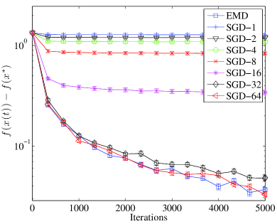
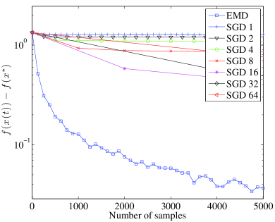
Figure 1: Performance of the EMD algorithm (5) on a robust system identification task where data is generated according to an autoregressive process.

As a natural representative from the multiple-replications family of algorithms, we use the classical stochastic gradient descent (SGD) algorithm (in the form studied by Nemirovski et al. [30]). To generate each sample for SGD, we begin with the point $\xi_{1}^{1}=0$ and perform $k$ of steps of the procedure (29), using $\xi_{k}^{\{1,2\}}$ to compute subgradients for SGD. For EMD, we use the proximal function $\psi(x)=\frac{1}{2}\left\|{x}\right\|_{2}^{2}$, which yields the direct analogue of stochastic gradient descent. To measure the objective value $f(x)$, we generate an independent fixed sample of size $N=10^{5}$ from the process (29), using $f(x)\approx\frac{1}{N}\sum_{i=1}^{N}F(x;\xi_{i})$. For each algorithm, to choose the stepsize multiplier $\alpha\propto R/G$, we estimate $G$ by taking 100 samples $\xi_{t}^{1}$ and computing the empirical average of $\|{\xi_{t}^{1}}\|_{2}^{2}$. For EMD, we deliberately underestimate the mixing time by the constant $1$ (other estimates of the mixing time yielded similar performance).

In Figure 1, we show the convergence behavior (as a function of number of samples) for the EMD algorithm compared with the behavior of the stochastic gradient method for different numbers $k$ of initial simulation steps before obtaining the sample $\xi$ used in each iteration of SGD. The line in each plot corresponding to SGD-$k$ shows the convergence of stochastic gradient descent as a function of number of iterations when $k$ initial samples are used for each independent sample $\xi$. The left plot in Figure 1 makes clear that if the mixing time is underestimated, the multiple-replications approach fails. As demonstrated by our theory, however, EMD still guarantees convergence even with poor stepsize choices (see also our experiments in the next section). For large enough mixing time estimate $k$, the multiple-replication stochastic gradient method and the EMD method have comparable performance in terms of optimization error as a function of number of gradient steps. The right plot in Figure 1 shows the convergence behavior of the competing methods as a function of the number of samples of the stochastic process (29). From this plot, it becomes clear that using each sample sequentially as in EMD—rather than attempting to draw independent samples at each iteration—is the more computationally efficient approach.

5.2 Robustness and non-Euclidean geometry

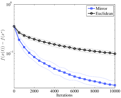
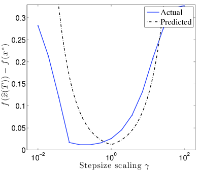
Figure 2: Left: optimization error on a statistical machine learning task of the Euclidean variant of the EMD algorithm (5) versus that of the $\ell_{p}$-norm variant with $\psi(x)=\frac{1}{2}\left\|x\right\|_{p}^{2}$, $p=1+1/\log d$, plotted against number of iterations. Right: robustness of the EMD algorithm (5) to modifications in the choice of stepsize.

In our second numerical experiment, we study an important problem that takes motivation from distributed statistical machine learning problems: the support vector machine problem [11], where the samples $\xi\in\mathbb{R}^{d}$ and the instantaneous objective is

$$F(x;\xi)=\left[{1-\left\langle\xi,x\right\rangle}\right]_{+}.$$

We study the performance of the EMD algorithm for the distributed Markov incremental mirror descent framework in § 4.1. In the notation of § 4.1, we simulate $n=50$ “processors,” and for each we draw a sample of $m=50$ samples according to the following process. Before performing any sampling, we set $u$ to be a random vector from $\{x\in\mathbb{R}^{d}:\left\|{x}\right\|_{1}\leq R\}$, where $R=5$ and $d=500$. To generate the $i$th data sample, we draw a vector $a_{i}\in\mathbb{R}^{d}$ with entries $a_{i,j}\in\{-1,1\}$ each with probability $\frac{1}{2}$, and set $b_{i}=\mathop{\rm sign}(\left\langle a_{i},u\right\rangle)$. With probability $.05$, we flip the sign of $b_{i}$ (this makes the problem slightly more difficult, as no vector $x$ will perfectly satisfy $b_{i}=\mathop{\rm sign}(\left\langle a_{i},x\right\rangle)$), and regardless we set $\xi_{i}=b_{i}a_{i}$. We thus generate a total of $N=nm=2500$ samples, and set the $i$th objective in the distributed minimization problem (17) to be

$$f_{i}(x)=\frac{1}{m}\sum_{k=m(i-1)+1}^{mi}F(x;\xi_{k})=\mathbb{E}_{\Pi_{i}}[F(x;\xi)]=\mathbb{E}_{\Pi_{i}}\left[\left[{1-\left\langle\xi,x\right\rangle}\right]_{+}\right],$$ (31)

where $\Pi_{i}$ denotes the uniform distribution over the $i$th block of $m$ samples. Our algorithm to minimize $f(x)=\frac{1}{n}\sum_{i=1}^{n}f_{i}(x)$ is the Markov analogue (18) of the general EMD algorithm (5). We minimize $f(x)$ over $\{x:\left\|{x}\right\|_{1}\leq R\}$ offline using standard LP software to obtain the optimal value $f(x^{\star})$ of the problem.

We use the objectives (31) to (i) understand the effectiveness of allowing non-Euclidean proximal functions $\psi$ in the update (5) and (ii) study the robustness of the EMD algorithm (5) to stepsize selection. We begin with the first goal. As noted by Ben-Tal et al. [4], the choice $\psi(x)=\frac{1}{2}\left\|x\right\|_{p}^{2}$ with $p=1+1/\log(d)$ yields a nearly optimal dependence on dimension in non-Euclidean gradient methods. Let $\tau_{\rm mix}$ denote the mixing time of the Markov chain (for Hellinger or total variation distance). Applying Corollary 3 and the analysis of Ben-Tal et al. with this choice of proximal function and $\alpha=R/\sqrt{\log(d)\tau_{\rm mix}}$ yields

$$\mathbb{E}[f(\widehat{x}(T))]-\inf_{x\in\mathcal{X}}f(x)=\mathcal{O}\left(\frac{R\sqrt{\tau_{\rm mix}\log d}}{\sqrt{T}}\right),$$

since $\left\|{\partial_{x}F(x;\xi)}\right\|_{\infty}\leq\left\|{\xi}\right\|_{\infty}=1$ by our sampling of the vectors $a_{i}\in\{-1,1\}^{d}$, and $R$ is the radius of $\mathcal{X}$ in $\ell_{1}$-norm. Compared to the Euclidean variant [20, 34] with $\psi(x)=\frac{1}{2}\left\|{x}\right\|_{2}^{2}$, whose convergence rate also follows from Corollary 3, this is an improvement of $\sqrt{d/\log d}$, since $\left\|{\partial_{x}F(x;\xi)}\right\|_{2}$ can be as large as $\sqrt{d}$.

We plot the results of 50 simulations of the distributed minimization problem in the left plot of Figure 2. For our underlying network topology, we use a $4$-connected cycle (each node in the cycle is connected to its $4$ neighbors on the right and left) and $n=50$ nodes. The line of blue squares is the mirror-descent approach with $\psi(x)=\frac{1}{2}\left\|x\right\|_{p}^{2}$ with $p=1+1/\log(d)$ (we use $d=500$), while the black line of circles denotes the Euclidean variant with $\psi(x)=\frac{1}{2}\left\|{x}\right\|_{2}^{2}$. The dotted lines below and above each plot give the $5$th and $95$th percentiles, respectively, of the optimization error across all simulations. For each algorithm, we use the optimal step size setting $\alpha(t)$ predicted by our theory (recall Corollary 3). It is clear that the non-Euclidean variant enjoys better performance, as our theory (and previous work on the dimension dependence of mirror descent [31, 30, 4, 3]) suggests.

The final simulation we perform is on the same problem, but we investigate the robustness of the EMD algorithm to mis-specified stepsizes. We take the stepsize $\alpha^{*}$ predicted by our theory (Corollary 3), and use $\alpha(t)=\gamma\alpha^{*}/\sqrt{t}$ for values of $\gamma$ uniformly logarithmically spaced from $\gamma=10^{-2}$ to $\gamma=10^{2}$. The plot on the right side of Figure 2 shows the mean optimality gap of $\widehat{x}(T)$ after $T=10000$ iterations for different values of $\gamma$, along with standard deviations, across 50 experiments. The black dotted line shows the predicted optimality gap as a function of the mis-specification (recall our discussion on robustness following Corollary 2). The EMD algorithm is certainly affected by mis-specification of the initial stepsize, though for a range of values of roughly $\gamma=10^{-1}$ to $\gamma=10$, the performance degradation does not appear extraordinary. In addition, our experiments show that our theoretical predictions appear to capture the empirical behavior of the method quite well.

6 Analysis

In this section, we analyze the convergence of the EMD algorithm from Section 2. Our first subsection lays the groundwork, gives necessary notation, and provides a few optimization-based results. The second subsection contains the proofs of results on expected rates of convergence, while the third subsection shows how to achieve convergence guarantees with high probability. The fourth subsection shows the convergence of the EMD method under probabilistic (random) mixing times, while the final subsection proves the order-optimality of the EMD method.

6.1 Definitions, assumptions, and optimization-based results

To state our results formally, we begin by giving a few standard definitions and collecting a few consequences of Assumptions A and B that make our proofs cleaner. Recall the measurable selection $\mathsf{G}$, where $\mathsf{G}(x;\xi)\in\partial_{x}F(x;\xi)$ represents a fixed and measurable element of the subgradient of $F(\cdot;\xi)$ evaluated at $x$, and the EMD algorithm (5) has $g(t)=\mathsf{G}(x(t);\xi_{t})$. By our assumptions on $F$, for any distribution $Q$ for which the expectations below are defined, expectation and subdifferentiation commute [37, 5]:

$$f_{Q}(x):=\mathbb{E}_{Q}[F(x;\xi)]=\int_{\Xi}F(x;\xi)dQ(\xi)~{}~{}~{}\mbox{then}~{}~{}~{}\partial f_{Q}(x)=\mathbb{E}_{Q}[\partial F(x;\xi)].$$

In particular, $\mathbb{E}_{\Pi}[\partial F(x;\xi)]=\partial f(x)$ and $\mathbb{E}_{\Pi}[\mathsf{G}(x;\xi)]\in\partial f(x)$. In addition, the compactness assumption that $D_{\psi}(x^{\star},x(t))\leq\frac{1}{2}R^{2}$ for all $t$ coupled with the strong convexity of $\psi$ implies

$$\left\|x(t)-x^{\star}\right\|^{2}\leq 2D_{\psi}(x^{\star},x(t))\leq R^{2}~{}~{}~{}\mbox{so}~{}~{}~{}\left\|x(t)-x^{\star}\right\|\leq R.$$ (32)

We now provide two relatively standard optimization-theoretic results that make our proofs substantially easier. To make the presentation self-contained, we give proofs of these results in Appendix A. The two lemmas are essentially present in earlier work [31, 3], but our stochastic setting requires a bit of care.

Lemma 10.

Let $x(t)$ be defined by the EMD update (5). For any $\tau\in\mathbb{N}$ and any $x^{\star}\in\mathcal{X}$,

$$\sum_{t=\tau+1}^{T}F(x(t);\xi_{t})-F(x^{\star};\xi_{t})\leq\frac{1}{2\alpha(T)}R^{2}+\sum_{t=\tau+1}^{T}\frac{\alpha(t)}{2}\left\|g(t)\right\|_{*}^{2}.$$

Lemma 11.

Let $x(t)$ be generated according to the EMD algorithm (5). Then

$$\left\|x(t)-x(t+1)\right\|\leq\alpha(t)\left\|g(t)\right\|_{*}.$$

6.2 Expected convergence rates

Now that we have established the relevant optimization-based results and setup in Section 6.1, the proof of Theorem 1 requires that we understand the impact of the ergodic sequence $\xi_{1},\xi_{2},\ldots$ on the EMD procedure. The key equality that allows us to prove Theorems 1 and 2 is the following: for any $\tau\geq 0$,

$$\sum_{t=1}^{T}f(x(t))-f(x^{\star}) =\sum_{t=1}^{T-\tau}f(x(t))-f(x^{\star})-F(x(t);\xi_{t+\tau})+F(x^{\star};\xi_{t+\tau})$$

$$\quad~{}+\sum_{t=1}^{T-\tau}F(x(t);\xi_{t+\tau})-F(x(t+\tau);\xi_{t+\tau})$$ (33)

$$\quad~{}+\sum_{t=\tau+1}^{T}F(x(t);\xi_{t})-F(x^{\star};\xi_{t})+\sum_{t=T-\tau+1}^{T}f(x(t))-f(x^{\star}).$$

We may set $\tau=0$ in the expression (33), taking expectations and applying Lemma 10, to recover the known convergence rates [30] for the stochastic gradient method with independent samples. However, the essential idea that the expansion (33) allows us to implement is that for large enough $\tau$, the sample $\xi_{t+\tau}$ is nearly “independent” of the parameters $x(t)$, since the stochastic process $P$ is mixing. By allowing $\tau>0$, we can bound the four sums (33) using a combination of Lemmas 10 and 11, then apply the mixing properties of the stochastic process $P$ to show that $F(x(t);\xi_{t+\tau})$ is a nearly unbiased estimate of $f(x(t))$:

$$\mathbb{E}[f(x(t))-F(x(t);\xi_{t+\tau})]\approx 0.$$

We formalize this intuition with two lemmas, whose proofs we provide in Appendix B.

Lemma 12.

Let $x$ be $\mathcal{F}_{t}$-measurable and $\tau\geq 1$. If Assumption A holds,

$$\left|\mathbb{E}\left[f(x)-f(x^{\star})-F(x;\xi_{t+\tau})+F(x^{\star};\xi_{t+\tau})\mid\mathcal{F}_{t}\right]\right|\leq 3GR\cdot d_{\rm hel}\left(P_{[t]}^{t+\tau},\Pi\right).$$

If Assumption B holds,

$$\left|\mathbb{E}\left[f(x)-f(x^{\star})-F(x;\xi_{t+\tau})+F(x^{\star};\xi_{t+\tau})\mid\mathcal{F}_{t}\right]\right|\leq GR\cdot d_{{}_{\rm TV}}\left(P_{[t]}^{t+\tau},\Pi\right).$$

The next lemma applies a type of stability argument, showing that function values between $x(t)$ and $x(t+\tau)$ cannot be too far apart.

Lemma 13.

Let $\tau\geq 0$ and $\alpha(t)$ be non-increasing. If Assumption A holds, then

$$\mathbb{E}[F(x(t);\xi_{t+\tau})-F(x(t+\tau);\xi_{t+\tau})\mid\mathcal{F}_{t-1}]\leq\tau\alpha(t)G^{2}.$$

If Assumption B holds, then

$$F(x(t);\xi_{t+\tau})-F(x(t+\tau);\xi_{t+\tau})\leq\tau\alpha(t)G^{2}.$$

We can now apply Lemmas 10–13 to give the promised proof of Theorem 1.

Proof of Theorem 1     The equality (33) is non-probabilistic, so all we need to complete the proof is to take expectations, applying the preceding lemmas. First, we map $\tau$ to $\tau-1$ in the previous results, which will make our analysis cleaner. Throughout this proof, the quantity $d(\cdot,\Pi)$ will denote $3d_{\rm hel}(\cdot,\Pi)$ when we apply Assumption A and will denote $d_{{}_{\rm TV}}(\cdot,\Pi)$ when using Assumption B, as the proof is identical in either case. We control the expectation of each of the four sums (33) in turn. First, we apply Lemma 12 to see that

$$\sum_{t=1}^{T-\tau+1}\mathbb{E}[f(x(t))-f(x^{\star})-F(x(t);\xi_{t+\tau-1})+F(x^{\star};\xi_{t+\tau-1})]\leq GR\sum_{t=0}^{T-\tau+1}\mathbb{E}[d(P_{[t]}^{t+\tau},\Pi)].$$

The second of the four sums (33) requires Lemma 13, which yields

$$\sum_{t=1}^{T-\tau+1}\mathbb{E}[F(x(t);\xi_{t+\tau-1})-F(x(t+\tau-1);\xi_{t+\tau-1})]\leq(\tau-1)G^{2}\sum_{t=1}^{T-\tau+1}\alpha(t).$$

Lemma 10 controls the third term in the series (33), and taking expectations gives $\mathbb{E}[\left\|g(t)\right\|_{*}^{2}]\leq G^{2}$. The final term in the sum (33) is bounded by $(\tau-1)RG$ when either of the Lipschitz assumptions A or B hold. Summing our four bounds, we obtain that for any $\tau\geq 1$,

$$\mathbb{E}\bigg{[}\sum_{t=1}^{T}f(x(t))-f(x^{\star})\bigg{]} \leq GR\sum_{t=1}^{T-\tau+1}\mathbb{E}\left[d\left(P_{[t-1]}^{t+\tau-1},\Pi\right)\right]+\frac{R^{2}}{2\alpha(T)}+\frac{G^{2}}{2}\sum_{t=\tau}^{T}\alpha(t)$$

$$\qquad~{}+(\tau-1)G^{2}\sum_{t=1}^{T-\tau+1}\alpha(t)+(\tau-1)RG.$$ (34)

Assumption C states that there exists a uniform mixing time $\tau_{\rm mix}(P,\epsilon)$ (for both total variation and Hellinger mixing) such that $d(P_{[t-1]}^{t+\tau-1},\Pi)\leq\epsilon$. Applying the definition of $\tau_{\rm mix}$ for Hellinger or total variation mixing completes the proof. ∎

6.3 High-probability convergence

In this section, we complement the convergence bounds in Section 6.2 with high-probability statements. We use martingale theory to show that the bound of Theorem 1 holds with high probability. We begin from the same starting point as the proof of Theorem 1—with the expansion (33)—but now we show that the random sum

$$\sum_{t=1}^{T-\tau+1}f(x(t))-f(x^{\star})-F(x(t);\xi_{t+\tau-1})+F(x^{\star};\xi_{t+\tau-1})$$ (35)

is small with high probability. Intuitively, this follows because given the initial $t-\tau$ samples $\xi_{1},\ldots,\xi_{t-\tau}$, the $t$th sample $\xi_{t}$ is almost a sample from the stationary distribution $\Pi$. With this in mind, we can show that an appropriately subsampled version of the above sequence behaves approximately as a martingale, and we can then apply Azuma’s inequality [2] to derive high-probability guarantees on the sum (35).

Proposition 1.

Let Assumption B hold and $\delta\in(0,1)$. With probability at least $1-\delta$, for $\tau\in\mathbb{N}$ with $\tau\in[1,T/2]$,

$$\sum_{t=1}^{T-\tau+1}\left[f(x(t))-F(x(t);\xi_{t+\tau-1})+F(x^{\star};\xi_{t+\tau-1})-f(x^{\star})\right]$$

$$\qquad\qquad\qquad~{}\leq 4GR\sqrt{T\tau\log\frac{\tau}{\delta}}+GR\sum_{t=1}^{T}d_{{}_{\rm TV}}\left(P_{[t-\tau]}^{t},\Pi\right).$$

We provide a proof in Appendix C and can now prove Theorem 2.

Proof of Theorem 2     The proof is a combination of the proofs of previous results. Starting from the expansion (33), we use Lemma 13 to see that

$$\sum_{t=1}^{T-\tau+1}F(x(t);\xi_{t+\tau-1})-F(x(t+\tau-1);\xi_{t+\tau-1})\leq(\tau-1)G^{2}\sum_{t=1}^{T-\tau+1}\alpha(t),$$

and applying the $G$-Lipschitz continuity of the functions $F(\cdot;\xi)$ and compactness of $\mathcal{X}$ we obtain

$$\sum_{t=T-\tau+2}^{T}f(x(t))-f(x^{\star})\leq(\tau-1)GR.$$

In addition, the convergence guarantee in Lemma 10 guarantees that

$$\sum_{t=\tau}^{T}F(x(t);\xi_{t})-F(x^{\star};\xi_{t})\leq\frac{1}{2\alpha(T)}R^{2}+\frac{G^{2}}{2}\sum_{t=1}^{T}\alpha(t).$$

Combining these bounds, we can replace the equality (33) with the bound

$$\sum_{t=1}^{T}f(x(t))-f(x^{\star}) \leq\frac{1}{2\alpha(T)}R^{2}+\frac{G^{2}}{2}\sum_{t=1}^{T}\alpha(t)+(\tau-1)\bigg{[}GR+G^{2}\sum_{t=1}^{T}\alpha(t)\bigg{]}$$ (36)

$$\quad~{}+\sum_{t=1}^{T-\tau+1}\left[f(x(t))-F(x(t);\xi_{t+\tau-1})+F(x^{\star};\xi_{t+\tau-1})-f(x^{\star})\right],$$

which holds for any $\tau\geq 1$. What remains is to replace the last term in the non-probabilistic bound (36) with the upper bound in Proposition 1, which holds with probability $1-\delta$, and then to replace $\tau$ with $\tau_{{}_{\rm TV}}(P,\epsilon)$, which guarantees the inequality $d_{{}_{\rm TV}}(P_{[t-\tau]}^{t},\Pi)\leq\epsilon$. ∎

6.4 Random mixing

In this section, we give the proof of Theorem 3. The proof is similar to that of Theorem 2, but we need an auxiliary lemma that allows us to guarantee that the mixing times are bounded uniformly for all times and for all desired accuracies of mixing $\epsilon$. See Appendix D for the proof of the lemma.

Lemma 14.

Let Assumption D hold and $\delta\in(0,1)$. With probability at least $1-\delta$,

$$\max_{s\in\{1,\ldots,T\}}\sup_{\{\epsilon\,:\,\tau_{{}_{\rm TV}}(P,\epsilon)\leq T\}}\left(\tau_{{}_{\rm TV}}(P_{[s]},\epsilon)-\tau_{{}_{\rm TV}}(P,\epsilon)\right)\leq\kappa\left(\log\frac{1}{\delta}+2\log(T)\right).$$

Rewriting Lemma 14 slightly, we may define $\tau=\tau_{{}_{\rm TV}}(P,\epsilon)+\kappa(\log\frac{1}{\delta}+2\log(T))$, and we find that with probability at least $1-\delta$,

$$d_{{}_{\rm TV}}\left(P_{[s]}^{s+\tau},\Pi\right)\leq\epsilon$$ (37)

for all $s\in\{1,\ldots,T\}$ and for all $\epsilon>0$ with $\tau_{{}_{\rm TV}}(P,\epsilon)\leq T$. This leads us to

Proof of Theorem 3     All that is different in the proof of this theorem from that of Theorem 2 is that in the penultimate inequality (36), when we apply Proposition 1, we no longer have the guarantee that $d_{{}_{\rm TV}}(P_{[t-\tau]}^{t},\Pi)\leq\epsilon$ for all $t$. To that end, let $\epsilon$ be such that $\tau_{{}_{\rm TV}}(P,\epsilon)\leq T$. Apply Lemma 14 and its consequence (37), which states that if we take $\tau=\tau_{{}_{\rm TV}}(P,\epsilon)+\kappa(\log\frac{1}{\delta}+2\log(T))$, then we obtain that $d_{{}_{\rm TV}}(P_{[t-\tau]}^{t},\Pi)\leq\epsilon$ with probability at least $1-\delta$. If $\tau_{{}_{\rm TV}}(P,\epsilon)>T$, the bound in the theorem holds vacuously, so we may extend the result to all $\epsilon>0$. ∎

6.5 Lower bounds on optimization accuracy

Our proof of Theorem 4 mirrors the proof of Theorem 1 in the paper by Agarwal et al. [1], so we are somewhat terse in our description and proof. The intuition in the proof is that if the stochastic process $P$ returns a sample from the stationary distribution $\Pi$ every $\tau$ timesteps, otherwise returning a sample identical to the previous one, then the convergence rate of any algorithm should be a factor of $\tau$ slower than if it could receive independent samples from $\Pi$. Mesterharm [26] employs a similar approach to give a lower bound on the performance of online learning algorithms. More formally, by using an identical construction to [1, Section IV.A], we may reduce the problem of minimization of a function $f:\mathbb{R}^{d}\rightarrow\mathbb{R}$ to identifying the bias of $d$ coins. To that end, let $\mathcal{V}\subset\{-1,1\}^{d}$ be a packing of the $d$-dimensional hypercube such that $\nu,\nu^{\prime}\in\mathcal{V}$ with $\nu\neq\nu^{\prime}$ satisfy $\left\|\nu-\nu^{\prime}\right\|_{1}\geq d/2$; it is a classical fact [25] that there is such a set with cardinality $|\mathcal{V}|\geq(2e^{-\frac{1}{2}})^{d/2}$.

Now for a fixed $\tau\in\mathbb{N}$, consider the following sequential sampling procedure, which generates a set of pairs of random vectors $\{(U_{t},Y_{t})\}_{t=1}^{\infty}$. Choose a vector $\nu\in\mathcal{V}$ uniformly at random and let $\delta\in\left({0},{1/4}\right]$. Let $P_{\nu}$ denote the distribution (conditional on $\nu$) that corresponds to the following: for each $t$, construct samples according to

1. If $(t-1)\mod\tau\neq 0$, take $U_{t}=U_{t-1}$ and $Y_{t}=Y_{t-1}$.

2. Otherwise, pick a uniformly random subset $U_{t}\subset\{1,\ldots,d\}$ of size $|U_{t}|=m$, then

   1. For each $i\in U_{t}$, construct a random variable $C_{i}$ such that $C_{i}=1$ with probability $\frac{1}{2}+\nu_{i}\delta$ and $C_{i}=-1$ with probability $\frac{1}{2}-\nu_{i}\delta$.

   2. Construct the vector $Y_{t}\in\{-1,1\}^{d}$ such that $Y_{t,i}=C_{i}$ if $i\in U_{t}$, and otherwise $Y_{t,i}$ is uniform Bernoulli, that is, if $i\not\in U_{t}$ then $Y_{t,i}=1$ with probability $\frac{1}{2}$ and $Y_{t,i}=-1$ with probability $\frac{1}{2}$.

This sampling procedure yields a sequence $\xi_{t}=(U_{t},Y_{t})$, where if $\Pi_{\nu}$ is the distribution of a pair $(U,Y)$ such that $U\subset\{1,\ldots,d\}$ is chosen uniformly at random with size $|U|=m$ and $Y$ is sampled according to the steps (i)–(ii) above, then $\Pi_{\nu}$ is the stationary distribution of $P_{\nu}$. Moreover, we see that $d_{{}_{\rm TV}}(P_{[t]}^{t+\tau+k},\Pi)=0$ for any $k\geq 0$ and any $t$, since the distribution $P_{\nu}$ corresponds to receiving an independent sample $(U,Y)$ from $\Pi_{\nu}$ every $\tau$ steps.

Let $I(X;Y)$ denote the mutual information between random variables $X$ and $Y$ and let $H(X)$ denote the (Shannon) entropy of $X$. By inspection of Agarwal et al.’s proof [1, Lemma 3], since $\Pi_{\nu}$ is the stationary distribution of $P_{\nu}$, a tight enough bound on the mutual information $I((U_{1},Y_{1}),\ldots,(U_{T},Y_{T});\nu)$ proves Theorem 4. Hence, we provide the following lemma:

Lemma 15.

Let the sequence $\xi_{t}=(U_{t},Y_{t})$ be generated according to the steps (a)–(b) above. Then for $\delta\in\left({0},{1/4}\right]$,

$$I\left((U_{1},Y_{1}),\ldots,(U_{T},Y_{T});\nu\right)\leq 16\left\lceil{\frac{T}{\tau}}\right\rceil m\delta^{2}.$$

Proof    Our sampling model (a)–(b) sets blocks of size $\tau$ to be equal, that is, $(U_{1},Y_{1})=\cdots=(U_{\tau},Y_{\tau})$, $(U_{\tau+1},Y_{\tau+1})=\cdots=(U_{2\tau},Y_{2\tau})$, and so on, whereas different blocks are independent given the variable $\nu$. We thus see that by the definitions of mutual information, conditional entropy, and that entropy is sub-additive [12],

$$I\left((U_{1},Y_{1}),\ldots,(U_{T},Y_{T});\nu\right)$$

$$=H((U_{1},Y_{1}),\ldots,(U_{T},Y_{T}))-H((U_{1},Y_{1}),\ldots,(U_{T},Y_{T})\mid\nu)$$

$$=H((U_{1},Y_{1}),\ldots,(U_{T},Y_{T}))-\sum_{k=1}^{\left\lceil{T/\tau}\right\rceil}H\left((U_{(k-1)\tau+1},Y_{(k-1)\tau+1}),\ldots,(U_{k\tau},Y_{k\tau})\mid\nu\right)$$

$$\leq\sum_{k=1}^{\left\lceil{T/\tau}\right\rceil}\left[H\left((U_{(k-1)\tau+1},Y_{(k-1)\tau+1}),\ldots,(U_{k\tau},Y_{k\tau})\right)-H\left((U_{(k-1)\tau+1},Y_{(k-1)\tau+1}),\ldots,(U_{k\tau},Y_{k\tau})\mid\nu\right)\right]$$

$$=\sum_{k=1}^{\left\lceil{T/\tau}\right\rceil}I\left((U_{(k-1)\tau+1},Y_{(k-1)\tau+1}),\ldots,(U_{k\tau},Y_{k\tau});\nu\right)=\sum_{k=1}^{\left\lceil{T/\tau}\right\rceil}I\left((U_{k\tau},Y_{k\tau});\nu\right).$$ (38)

In the last line we have used that within the same block of size $\tau$, all $(U_{t},Y_{t})$ pairs are equal. Now, using the bound (38), we apply an identical derivation as that given in the proof of Agarwal et al.’s Lemma 3 (following Eq. (25) there). For any fixed $k$ we have $I((U_{k\tau},Y_{k\tau});\nu)\leq 16m\delta^{2}$, which completes the proof of the lemma. ∎

Proof of Theorem 4     Use Agarwal et al.’s construction (see Eq. (16) in Section IV.A of [1]) of a “difficult” subclass of functions, then in the proof of Theorem 1 from [1], replace their coin-flipping oracle with the steps (a)–(b) and applications of their Lemma 3 with Lemma 15 above. ∎

7 Conclusions

In this paper, we have shown that stochastic subgradient and mirror descent approaches extend in an elegant way to situations in which we have no access to i.i.d. samples from the desired distribution. In spite of this difficulty, we are able to achieve reasonably fast rates of convergence for the ergodic mirror descent algorithm—the natural extension of stochastic mirror descent—under reasonable assumptions on the ergodicity of the stochastic process $\{\xi_{t}\}$ that generates the samples. We gave several examples showing the strengths and uses of our new analysis, and believe that there are many more. In addition, our results give a relatively clean and simple way to derive finite sample rates of convergence for statistical estimators with dependent data without requiring the full machinery of empirical process theory (e.g., [42]). Though we have provided lower bounds showing that our analysis is tight to numerical constants, it may be possible to sharpen our results for interesting special cases, such as when the distribution of the stochastic process $\{\xi_{t}\}$ has nice enough Markovianity properties. We leave such questions to future work.

Acknowledgments

We thank Lester Mackey for several interesting questions he posed that helped lead to this work. In addition, we thank the three anonymous reviewers and the editor for many insightful comments and suggestions.

Appendix A Proofs of Optimization Results

Proof of Lemma 10     The proof of the lemma begins by controlling the amount of progress made by one step of the EMD method, then summing the resulting bound. By the first-order convexity inequality and definition of the subgradient $g(t)$, we have

$$F(x(t);\xi_{t})-F(x^{*};\xi_{t}) \leq\left\langle g(t),x(t)-x^{*}\right\rangle$$

$$=\left\langle g(t),x(t+1)-x^{*}\right\rangle+\left\langle g(t),x(t+1)-x(t)\right\rangle.$$ (39)

For $y\in\mathcal{X}$, the first-order optimality conditions for $x(t+1)$ in the update (5) imply

$$\left\langle\alpha(t)g(t)+\nabla\psi(x(t+1))-\nabla\psi(x(t)),y-x(t+1)\right\rangle\geq 0.$$

In particular, we can take $y=x^{*}$ in this bound to find

$$\alpha(t)\left\langle g(t),x(t+1)-x^{*}\right\rangle\leq\left\langle\nabla\psi(x(t+1))-\nabla\psi(x(t)),x^{*}-x(t+1)\right\rangle.$$ (40)

Now we use the definition of the Bregman divergence $D_{\psi}$, to obtain

$$\left\langle\nabla\psi(x(t+1))-\nabla\psi(x(t)),x^{*}-x(t+1)\right\rangle$$

$$\qquad\qquad\qquad\qquad~{}=D_{\psi}(x^{*},x(t))-D_{\psi}(x^{*},x(t+1))-D_{\psi}(x(t+1),x(t)).$$

Combining this result with the expanded gradient term (39) and the the first-order convexity inequality (40), we get

$$F(x(t);\xi_{t})-F(x^{*};\xi_{t})\leq\frac{1}{\alpha(t)}D_{\psi}(x^{*},x(t))-\frac{1}{\alpha(t)}D_{\psi}(x^{*},x(t+1))$$

$$\qquad\qquad\qquad\qquad\qquad\quad~{}-\frac{1}{\alpha(t)}D_{\psi}(x(t+1),x(t))+\left\langle g(t),x(t+1)-x(t)\right\rangle$$

$$\qquad\qquad\stackrel{{\scriptstyle(i)}}{{\leq}}\frac{1}{\alpha(t)}D_{\psi}(x^{*},x(t))-\frac{1}{\alpha(t)}D_{\psi}(x^{*},x(t+1))-\frac{1}{\alpha(t)}D_{\psi}(x(t+1),x(t))$$

$$\qquad\qquad\quad~{}+\frac{\alpha(t)}{2}\left\|g(t)\right\|_{*}^{2}+\frac{1}{2\alpha(t)}\left\|x(t+1)-x(t)\right\|^{2}$$

$$\qquad\qquad\stackrel{{\scriptstyle(ii)}}{{\leq}}\frac{1}{\alpha(t)}D_{\psi}(x^{*},x(t))-\frac{1}{\alpha(t)}D_{\psi}(x^{*},x(t+1))+\frac{\alpha(t)}{2}\left\|g(t)\right\|_{*}^{2}.$$

The inequality $(i)$ is a consequence of the Fenchel-Young inequality applied to the conjugates $\frac{1}{2}\left\|\cdot\right\|^{2}$ and $\frac{1}{2}\left\|\cdot\right\|_{*}^{2}$ (see, e.g., [8, Example 3.27]), while the inequality $(ii)$ follows by the strong convexity of $\psi$, which gives $D_{\psi}(x(t+1),x(t))\geq\frac{1}{2}\left\|x(t+1)-x(t)\right\|^{2}$.

Summing the final inequality, we obtain

$$\sum_{t=\tau+1}^{T}\left[F(x(t);\xi_{t})-F(x^{*};\xi_{t})\right]$$

$$\qquad\leq\sum_{t=\tau+1}^{T}\frac{1}{\alpha(t)}\left[D_{\psi}(x^{*},x(t))-D_{\psi}(x^{*},x(t+1))\right]+\sum_{t=\tau+1}^{T}\frac{\alpha(t)}{2}\left\|g(t)\right\|_{*}^{2}.$$

Using the compactness assumption that $D_{\psi}(x^{*},x)\leq\frac{1}{2}R^{2}$ for all $x\in\mathcal{X}$, we have

$$\sum_{t=\tau+1}^{T}\frac{1}{\alpha(t)}\left[D_{\psi}(x^{*},x(t))-D_{\psi}(x^{*},x(t+1))\right]$$

$$\leq\sum_{t=\tau+2}^{T}D_{\psi}(x^{*},x(t))\left[\frac{1}{\alpha(t)}-\frac{1}{\alpha(t-1)}\right]+\frac{1}{\alpha(\tau+1)}D_{\psi}(x^{*},x(\tau+1))$$

$$\leq\frac{R^{2}}{2}\sum_{t=\tau+2}^{T}\left[\frac{1}{\alpha(t)}-\frac{1}{\alpha(t-1)}\right]+\frac{1}{2\alpha(\tau+1)}R^{2}=\frac{R^{2}}{2\alpha(T)},$$

where for the last inequality we used that the stepsizes $\alpha(t)$ are non-increasing. ∎

Proof of Lemma 11     By the first-order condition for the optimality of $x(t+1)$ for the update (5), we have

$$\left\langle\alpha(t)g(t)+\nabla\psi(x(t+1))-\nabla\psi(x(t)),x(t)-x(t+1)\right\rangle\geq 0.$$

Rewriting, we have

$$\left\langle\nabla\psi(x(t))-\nabla\psi(x(t+1)),x(t)-x(t+1)\right\rangle \leq\alpha(t)\left\langle g(t),x(t)-x(t+1)\right\rangle$$

$$\leq\alpha(t)\left\|g(t)\right\|_{*}\left\|x(t)-x(t+1)\right\|$$

using Hölder’s inequality. Simple algebra shows that

$$D_{\psi}(x(t),x(t+1))+D_{\psi}(x(t+1),x(t))=\left\langle\nabla\psi(x(t))-\nabla\psi(x(t+1)),x(t)-x(t+1)\right\rangle,$$

and by the assumed strong convexity of $\psi$, we see

$$\left\|x(t)-x(t+1)\right\|^{2} \leq D_{\psi}(x(t+1),x(t))+D_{\psi}(x(t),x(t+1))$$

$$\leq\alpha(t)\left\|g(t)\right\|_{*}\left\|x(t)-x(t+1)\right\|.$$

Dividing by $\left\|x(t)-x(t+1)\right\|$ gives the desired result. ∎

Appendix B Mixing and expected function values

Proof of Lemma 12     Since $x\in\mathcal{F}_{t}$, we may integrate only against $\xi$ when taking expectations, which yields

$$\mathbb{E}\left[f(x)-f(x^{\star})-F(x;\xi_{t+\tau})+F(x^{\star};\xi_{t+\tau})\mid\mathcal{F}_{t}\right]$$

$$\quad=\int(F(x;\xi)-F(x^{\star};\xi))d\Pi(\xi)-\int(F(x;\xi)-F(x^{\star};\xi))dP^{t+\tau}_{[t]}(\xi).$$

Since we assume $P_{[s]}^{t}$ and $\Pi$ have densities $p_{[s]}^{t}$ and $\pi$ with respect to a measure $\mu$, this difference becomes $\int(F(x;\xi)-F(x^{\star};\xi))(\pi(\xi)-p_{[t]}^{t+\tau}(\xi))d\mu(\xi)$. Setting $p=p_{[t]}^{t+\tau}$ for shorthand, we obtain

$$\left|\int(F(x;\xi)-F(x^{\star};\xi))(\pi(\xi)-p(\xi))d\mu(\xi)\right|\leq\int|F(x;\xi)-F(x^{\star};\xi)|\left|p(\xi)-\pi(\xi)\right|d\mu(\xi)$$

$$=\int|F(x;\xi)-F(x^{\star};\xi)|\left(\sqrt{\pi(\xi)}+\sqrt{p(\xi)}\right)\left|\sqrt{\pi(\xi)}-\sqrt{p(\xi)}\right|d\mu(\xi)$$

$$\leq\sqrt{\int\left(F(x;\xi)-F(x^{\star};\xi)\right)^{2}\left(\sqrt{\pi(\xi)}+\sqrt{p(\xi)}\right)^{2}d\mu(\xi)\int\left(\sqrt{p(\xi)}-\sqrt{\pi(\xi)}\right)^{2}d\mu(\xi)}$$

$$=\sqrt{\int(F(x;\xi)-F(x^{\star};\xi))^{2}\left(\sqrt{\pi(\xi)}+\sqrt{p(\xi)}\right)^{2}d\mu(\xi)}\,d_{\rm hel}(P_{[t]}^{t+\tau},\Pi)$$

by Hölder’s inequality. Applying the inequality $(a+b)^{2}\leq 2a^{2}+2b^{2}$, valid for $a,b\in\mathbb{R}$, we obtain the further bound

$$\left(2\int\left(F(x;\xi)-F(x^{\star};\xi)\right)^{2}(\pi(\xi)+p(\xi))d\mu(\xi)\right)^{\frac{1}{2}}d_{\rm hel}(P_{[t]}^{t+\tau},\Pi)=$$ (41)

$$\sqrt{2}\left(\mathbb{E}_{\Pi}[\left(F(x;\xi)-F(x^{\star};\xi)\right)^{2}]+\mathbb{E}[\left(F(x;\xi_{t+\tau})-F(x^{\star};\xi_{t+\tau})\right)^{2}\mid\mathcal{F}_{t}]\right)^{\frac{1}{2}}d_{\rm hel}(P_{[t]}^{t+\tau},\Pi).$$

To control the expectation terms in the bound (41), we now use Assumption A. By the ($P$-almost sure) convexity of the function $x\mapsto F(x;\xi)$, we observe that

$$F(x;\xi)-F(x^{\star};\xi)\leq\left\langle\mathsf{G}(x;\xi),x-x^{\star}\right\rangle~{}~{}~{}\mbox{and}~{}~{}~{}F(x^{\star};\xi)-F(x;\xi)\leq\left\langle\mathsf{G}(x^{\star};\xi),x^{\star}-x\right\rangle.$$

Combining these two inequalities, we see that

$$\left(F(x;\xi)-F(x^{\star};\xi)\right)^{2} \leq\max\left\{\left\langle\mathsf{G}(x;\xi),x-x^{\star}\right\rangle^{2},\left\langle\mathsf{G}(x^{\star};\xi),x^{\star}-x\right\rangle^{2}\right\}$$

$$\leq\max\left\{\left\|\mathsf{G}(x;\xi)\right\|_{*}^{2},\left\|\mathsf{G}(x^{\star};\xi)\right\|_{*}^{2}\right\}\left\|x-x^{\star}\right\|^{2}$$

$$\leq\max\left\{\left\|\mathsf{G}(x;\xi)\right\|_{*}^{2},\left\|\mathsf{G}(x^{\star};\xi)\right\|_{*}^{2}\right\}R^{2},$$

where the last inequality uses our compactness assumption (4). Now we invoke Assumption A combined with the above inequality to obtain the further bound

$$\mathbb{E}\left[\left(F(x;\xi_{t+\tau})-F(x^{\star};\xi_{t+\tau})\right)^{2}\mid\mathcal{F}_{t}\right]$$

$$\qquad\leq R^{2}\mathbb{E}\left[\left\|\mathsf{G}(x;\xi_{t+\tau})\right\|_{*}^{2}+\left\|\mathsf{G}(x^{\star};\xi_{t+\tau})\right\|_{*}^{2}\mid\mathcal{F}_{t}\right]\leq 2G^{2}R^{2}.$$

An analogous argument yields the same bound for the expectation under the stationary distribution, so based on our earlier bound (41) we have

$$\left|\int(F(x;\xi)-F(x^{\star};\xi))\left(d\Pi(\xi)-dP_{[t]}^{t+\tau}(\xi)\right)\right|$$

$$\leq\int|F(x;\xi)-F(x^{\star};\xi)|\left|d\Pi(\xi)-dP_{[t]}^{t+\tau}(\xi)\right|\leq\sqrt{8G^{2}R^{2}}\,d_{\rm hel}\left(P_{[t]}^{t+\tau},\Pi\right).$$

This completes the proof of the first statement of the lemma.

The second statement is simpler: apply Assumption B to obtain

$$\left|\int(F(x;\xi)-F(x^{\star};\xi))(\pi(\xi)-p(\xi))d\mu(\xi)\right|\leq GR\int|p(\xi)-\pi(\xi)|d\mu(\xi).$$

Observing that the above bound is equal to $GRd_{{}_{\rm TV}}\left(P_{[t]}^{t+\tau},\Pi\right)$ completes the proof. ∎

Proof of Lemma 13     For any $x$ measurable with respect to the $\sigma$-field $\mathcal{F}_{s}$, we can define the function $h_{[s]}(x)=\mathbb{E}[F(x;\xi_{s+1})\mid\mathcal{F}_{s}]$. Assumption A implies that $h_{[s]}$ is a $G$-Lipschitz continuous function so long as its argument is $\mathcal{F}_{s}$-measurable, that is, $|h_{[s]}(x)-h_{[s]}(y)|\leq G\left\|x-y\right\|$ for $x,y\in\mathcal{F}_{s}$. In turn, this implies that

$$\mathbb{E}[F(x(t);\xi_{t+\tau})-F(x(t+\tau);\xi_{t+\tau})\mid\mathcal{F}_{t-1}]$$

$$\qquad=\sum_{s=t}^{t+\tau-1}\mathbb{E}[F(x(s);\xi_{t+\tau})-F(x(s+1);\xi_{t+\tau})\mid\mathcal{F}_{t-1}]$$

$$\qquad=\sum_{s=t}^{t+\tau-1}\mathbb{E}\left[\mathbb{E}[F(x(s);\xi_{t+\tau})-F(x(s+1);\xi_{t+\tau})\mid\mathcal{F}_{t+\tau-1}]\mid\mathcal{F}_{t-1}\right]$$

$$\qquad\leq\sum_{s=t}^{t+\tau-1}\mathbb{E}\left[G\left\|x(s)-x(s+1)\right\|\mid\mathcal{F}_{t-1}\right]$$

since $x(s)$ is $\mathcal{F}_{t+\tau-1}$-measurable for $s\leq t+\tau$. Now we apply Lemma 11, which shows that $\left\|x(s)-x(s+1)\right\|\leq\alpha(s)\left\|g(s)\right\|_{*}$, and we have the further inequality

$$\mathbb{E}[F(x(t);\xi_{t+\tau})-F(x(t+\tau);\xi_{t+\tau})\mid\mathcal{F}_{t-1}]\leq\sum_{s=t}^{t+\tau-1}G\alpha(s)\mathbb{E}[\left\|g(s)\right\|_{*}\mid\mathcal{F}_{t-1}].$$

Applying Jensen’s inequality and Assumption A, we see that

$$\mathbb{E}[\left\|g(s)\right\|_{*}\mid\mathcal{F}_{t-1}]\leq\sqrt{\mathbb{E}[\mathbb{E}[\left\|g(s)\right\|_{*}^{2}\mid\mathcal{F}_{s-1}]\mid\mathcal{F}_{t-1}]}\leq\sqrt{G^{2}}=G.$$

In conclusion, we have the first statement of the lemma:

$$\mathbb{E}[F(x(t);\xi_{t+\tau})-F(x(t+\tau);\xi_{t+\tau})\mid\mathcal{F}_{t-1}]\leq G^{2}\sum_{s=t}^{t+\tau-1}\alpha(s)\leq G^{2}\tau\alpha(t),$$

since the sequence $\alpha(t)$ is non-increasing. The proof of the second statement is entirely similar, but we do not need to apply conditional expectations. ∎

Appendix C Proof of Proposition 1

Proof of Proposition 1     We construct a family of $\tau$ different martingales from the summation in the statement of the proposition, each of which we control with high probability. Applying a union bound gives us control on the deviation of the entire series. We begin by defining the random variables

$$Z_{t}:=f(x(t-\tau+1))-F(x(t-\tau+1);\xi_{t})+F(x^{\star};\xi_{t})-f(x^{\star}),$$

noting that

$$\sum_{t=\tau}^{T}Z_{t}=\sum_{t=1}^{T-\tau+1}\left[f(x(t))-F(x(t);\xi_{t+\tau-1})+F(x^{\star};\xi_{t+\tau-1})-f(x^{\star})\right].$$

By defining the filtration of $\sigma$-fields $\mathcal{A}_{i}^{j}=\mathcal{F}_{\tau i+j}$ for $j=1,\ldots,\tau$, we can construct a set of Doob martingales $\{X_{1}^{j},X_{2}^{j},\ldots\}$ for $j=1,\ldots,\tau$ by making the definition

$$X_{i}^{j} :=Z_{\tau i+j}-\mathbb{E}[Z_{\tau i+j}\mid\mathcal{A}_{i-1}^{j}]=Z_{\tau i+j}-\mathbb{E}[Z_{\tau i+j}\mid\mathcal{F}_{\tau(i-1)+j}]$$

$$~{}=f(x(\tau(i-1)+j+1))-F(x(\tau(i-1)+j+1);\xi_{\tau i+j})$$

$$\qquad\quad~{}+F(x^{\star};\xi_{\tau i+j})-f(x^{\star})-\mathbb{E}[Z_{t}\mid\mathcal{F}_{\tau(i-1)+j}].$$

By inspection, $X_{i}^{j}$ is measurable with respect to the $\sigma$-field $\mathcal{A}_{i}^{j}$, and $\mathbb{E}[X_{i}^{j}\mid\mathcal{A}_{i-1}^{j}]=0$. So, for each $j$, the sequence $\{X_{i}^{j}:i=1,2,\ldots\}$ is a martingale difference sequence adapted to the filtration $\{\mathcal{A}_{i}^{j}:i=1,2,\ldots\}$. Define the index set $\mathcal{I}(j)$ to be the indices $\{1,\ldots,\left\lfloor{T/\tau}\right\rfloor+1\}$ for $j\leq T-\tau\left\lfloor{T/\tau}\right\rfloor$ and $\{1,\ldots,\left\lfloor{T/\tau}\right\rfloor\}$ otherwise. With the definition of $X_{i}^{j}$ and the indices $\mathcal{I}(j)$, we see that

$$\sum_{t=\tau}^{T}Z_{t}=\sum_{j=1}^{\tau}\sum_{i\in\mathcal{I}(j)}X_{i}^{j}+\sum_{t=\tau}^{T}\mathbb{E}[Z_{t}\mid\mathcal{F}_{t-\tau}]=\sum_{j=1}^{\tau}\sum_{i=1}^{|\mathcal{I}(j)|}X_{i}^{j}+\sum_{t=\tau}^{T}\mathbb{E}[Z_{t}\mid\mathcal{F}_{t-\tau}].$$ (42)

Now we note the following important fact: by the compactness assumption (32) and Assumption B, the $\mathcal{F}_{\tau(i-1)+j}$-measurability of $f(x(\tau(i-1)+j+1))$ implies

$$|X_{i}^{j}|=\left|Z_{\tau i+j}-\mathbb{E}[Z_{\tau i+j}\mid\mathcal{F}_{\tau(i-1)+j}]\right|\leq 2GR.$$

This bound, coupled with the representation (42), shows that $\sum_{t=\tau}^{T}Z_{t}$ is a sum of $\tau$ different bounded-difference martingales plus a sum of conditional expectations that we will bound later. To control the martingale portion of the sum (42), we apply the triangle inequality, a union bound, and Azuma’s inequality [2] to find

$$P\bigg{(}\sum_{j=1}^{\tau}\sum_{i\in\mathcal{I}(j)}X_{i}^{j}>\gamma\bigg{)} \leq\sum_{j=1}^{\tau}P\bigg{(}\sum_{i\in\mathcal{I}(j)}X_{i}^{j}>\frac{\gamma}{\tau}\bigg{)}\leq\sum_{j=1}^{\tau}\exp\left(-\frac{\gamma^{2}}{16G^{2}R^{2}\tau T}\right),$$

since there are fewer than $2T/\tau$ terms in each of the sums $X_{i}^{j}$ (by our assumption that $T/2\geq\tau$). Substituting $\gamma=4GR\sqrt{T\tau\log(\tau/\delta)}$, we find

$$P\bigg{(}\sum_{j=1}^{\tau}\sum_{i\in\mathcal{I}(j)}X_{i}^{j}>4GR\sqrt{T\tau\log\frac{\tau}{\delta}}\bigg{)}\leq\delta.$$

To bound the final term $\mathbb{E}[Z_{t}\mid\mathcal{F}_{t-\tau}]$ in the sum (42), we recall from Lemma 12 that

$$\left|\mathbb{E}[Z_{t}\mid\mathcal{F}_{t-\tau}]\right|\leq GR\cdot d_{{}_{\rm TV}}\left(P_{[t-\tau]}^{t},\Pi\right).$$

Summing this bound completes the proof. ∎

Appendix D Probabilistic Mixing

Proof of Lemma 5     Using the definitions in the statement of the lemma, take

$$\tau=\left\lfloor{\tau_{{}_{\rm TV}}(P,\epsilon)+\kappa c}\right\rfloor\geq\frac{\log\frac{1}{\epsilon}}{|\log\gamma|}+\frac{\log K}{|\log\gamma|}+\frac{c}{|\log\gamma|},$$

which implies by Markov’s inequality that

$$\mathbb{P}\left(d_{{}_{\rm TV}}\left(P_{[t]}^{t+\tau},\Pi\right)\geq\epsilon\right)\leq\frac{K\gamma^{\tau}}{\epsilon}\leq\frac{K\exp(-\log\frac{1}{\epsilon})\exp(-\log K)}{\epsilon}\exp(-c)=\exp(-c)$$

since $\gamma^{a/|\log\gamma|}=\exp(-a)$ for $0<\gamma<1$. Noting that

$$\mathbb{P}\left(\tau_{{}_{\rm TV}}(P_{[t]},\epsilon)>\tau\right)\leq\mathbb{P}\left(d_{{}_{\rm TV}}\left(P_{[t]}^{t+\tau},\Pi\right)>\epsilon\right)$$

for any $\tau\in\mathbb{N}$ completes the proof. ∎

Proof of Lemma 14     We use a covering number argument, which is common in uniform concentration inequalities in probability theory (e.g., [39]). For each $t\in\{1,\ldots,T\}$, define

$$\epsilon_{t}:=\inf\left\{\epsilon>0:\tau_{{}_{\rm TV}}(P,\epsilon)\leq t\right\}.$$

By the right-continuity of $\epsilon\mapsto\tau_{{}_{\rm TV}}(P,\epsilon)$, we have $\tau_{{}_{\rm TV}}(P,\epsilon_{t})\leq t$ but $\tau_{{}_{\rm TV}}(P,\epsilon_{t}-\delta)>t$ for any $\delta>0$. As a consequence, we see that for some $\epsilon\geq\epsilon_{T}$ to exist satisfying $\tau_{{}_{\rm TV}}(P_{[s]},\epsilon)>\tau_{{}_{\rm TV}}(P,\epsilon)+c$, it must be the case that

$$\tau_{{}_{\rm TV}}(P_{[s]},\epsilon_{t})-\tau_{{}_{\rm TV}}(P,\epsilon_{t})>c$$

for some $\epsilon_{t}$, where $t\in\{1,\ldots,T\}$. That is, we have

$$P\left(\tau_{{}_{\rm TV}}(P_{[s]},\epsilon)>\tau_{{}_{\rm TV}}(P,\epsilon)+c~{}\mbox{for~{}some~{}}s\in\{1,\ldots,T\}~{}\mbox{and}~{}\epsilon\geq\epsilon_{T}\right)$$

$$\qquad\qquad\qquad\qquad\qquad\qquad\qquad\qquad~{}\leq P\left(\max_{t,s\leq T}\left[\tau_{{}_{\rm TV}}(P_{[s]},\epsilon_{t})-\tau_{{}_{\rm TV}}(P,\epsilon_{t})\right]>c\right).$$

Applying a union bound and Assumption D, we thus see that for any $c\geq 0$,

$$P\left(\max_{s\leq T}\sup_{\epsilon\geq\epsilon_{T}}\left(\tau_{{}_{\rm TV}}(P_{[s]},\epsilon)-\tau_{{}_{\rm TV}}(P,\epsilon)\right)>c\right)$$

$$\qquad\leq T^{2}\max_{t,s\leq T}P\left(\tau_{{}_{\rm TV}}(P_{[s]},\epsilon_{t})>\tau_{{}_{\rm TV}}(P,\epsilon)+c\right)\leq T^{2}\exp\left(-c/\kappa\right).$$

Setting the final equation equal to $\delta$ and solving, we obtain $c=\kappa[\log(1/\delta)+2\log(T)]$, which is equivalent to the statement of the lemma. ∎

References

• [1] A. Agarwal, P. L. Bartlett, P. Ravikumar, and M. J. Wainwright. Information-theoretic lower bounds on the oracle complexity of convex optimization. IEEE Transactions on Information Theory, 58(5):3235–3249, May 2012.
• [2] K. Azuma. Weighted sums of certain dependent random variables. Tohoku Mathematical Journal, 68:357–367, 1967.
• [3] A. Beck and M. Teboulle. Mirror descent and nonlinear projected subgradient methods for convex optimization. Operations Research Letters, 31:167–175, 2003.
• [4] A. Ben-Tal, T. Margalit, and A. Nemirovski. The ordered subsets mirror descent optimization method with applications to tomography. SIAM Journal on Optimization, 12:79–108, 2001.
• [5] D. P. Bertsekas. Stochastic optimization problems with nondifferentiable cost functionals. Journal of Optimization Theory and Applications, 12(2):218–231, 1973.
• [6] P. Billingsley. Probability and Measure. Wiley, Second edition, 1986.
• [7] S. Boyd, A. Ghosh, B. Prabhakar, and D. Shah. Randomized gossip algorithms. IEEE Transactions on Information Theory, 52(6):2508–2530, 2006.
• [8] S. Boyd and L. Vandenberghe. Convex Optimization. Cambridge University Press, 2004.
• [9] R. C. Bradley. Basic properties of strong mixing conditions. a survey and some open questions. Probability Surveys, 2:107–144, 2005.
• [10] F. R. K. Chung. Spectral Graph Theory. AMS, 1998.
• [11] C. Cortes and V. Vapnik. Support-vector networks. Machine Learning, 20(3):273–297, September 1995.
• [12] T. M. Cover and J. A. Thomas. Elements of Information Theory. Wiley, 1991.
• [13] I. Csiszár. Information-type measures of difference of probability distributions and indirect observation. Studia Scientifica Mathematica Hungary, 2:299–318, 1967.
• [14] J. C. Duchi, A. Agarwal, and M. J. Wainwright. Dual averaging for distributed optimization: convergence analysis and network scaling. IEEE Transactions on Automatic Control, 57(3):592–606, 2012.
• [15] A. Gelman and D. B. Rubin. Inference from iterative simulation using multiple sequences. Statistical Science, 7(4):457–472, 1992.
• [16] J. Hiriart-Urruty and C. Lemaréchal. Convex Analysis and Minimization Algorithms I. Springer, 1996.
• [17] R. Impagliazzo and D. Zuckerman. How to recycle random bits. In 30th Annual Symposium on Foundations of Computer Science, pages 248–253, 1989.
• [18] S. Jarner and G. Roberts. Polynomial convergence rates of Markov chains. The Annals of Applied Probability, 12(1):pp. 224–247, 2002.
• [19] M. Jerrum and A. Sinclair. The Markov chain Monte Carlo method: an approach to approximate counting and integration. In D. S. Hochbaum, editor, Approximation Algorithms for NP-hard Problems. PWS Publishing, 1996.
• [20] B. Johansson, M. Rabi, and M. Johansson. A randomized incremental subgradient method for distributed optimization in networked systems. SIAM Journal on Optimization, 20(3):1157–1170, 2009.
• [21] A. Karzanov and L. Khachiyan. On the conductance of order Markov chains. Order, 8:7–15, 1991.
• [22] H. J. Kushner and G. Yin. Stochastic Approximation and Recursive Algorithms and Applications. Springer, Second edition, 2003.
• [23] V. Lesser, C. Ortiz, and M. Tambe, editors. Distributed Sensor Networks: A Multiagent Perspective, volume 9. Kluwer Academic Publishers, 2003.
• [24] E. Liebscher. Towards a unified approach for proving geometric ergodicity and mixing properties of nonlinear autoregressive processes. Journal of Time Series Analysis, 26(5):669–689, 2005.
• [25] J. Matousek. Lectures on Discrete Geometry. Springer, 2002.
• [26] C. Mesterharm. On-line learning with delayed feedback. In Algorithmic Learning Theory, pages 399–413, 2005.
• [27] S. Meyn and R. L. Tweedie. Markov Chains and Stochastic Stability. Cambridge University Press, Second edition, 2009.
• [28] A. Mokkadem. Mixing properties of ARMA processes. Stochastic Processes and their Applications, 29(2):309–315, 1988.
• [29] A. Nedić and D. P. Bertsekas. Incremental subgradient methods for nondifferentiable optimization. SIAM Journal on Optimization, 12:109–138, 2001.
• [30] A. Nemirovski, A. Juditsky, G. Lan, and A. Shapiro. Robust stochastic approximation approach to stochastic programming. SIAM Journal on Optimization, 19(4):1574–1609, 2009.
• [31] A. Nemirovski and D. Yudin. Problem Complexity and Method Efficiency in Optimization. Wiley, 1983.
• [32] B. T. Polyak and A. B. Juditsky. Acceleration of stochastic approximation by averaging. SIAM Journal on Control and Optimization, 30(4):838–855, 1992.
• [33] B. T. Polyak and J. Tsypkin. Robust identification. Automatica, 16:53–63, 1980.
• [34] S. S. Ram, A. Nedić, and V. V. Veeravalli. Incremental stochastic subgradient algorithms for convex optimization. SIAM Journal on Optimization, 20(2):691–717, 2009.
• [35] H. Robbins and S. Monro. A stochastic approximation method. Annals of Mathematical Statistics, 22:400–407, 1951.
• [36] C. Robert and G. Casella. Monte Carlo Statistical Methods. Springer, Second edition, 2004.
• [37] R. T. Rockafellar and R. J. B. Wets. On the interchange of subdifferentiation and conditional expectation for convex functionals. Stochastics: An International Journal of Probability and Stochastic Processes, 7:173–182, 1982.
• [38] J. C. Spall. Introduction to Stochastic Search and Optimization: Estimation, Simulation, and Control. Wiley, 2003.
• [39] V. N. Vapnik and A. Y. Chervonenkis. On the uniform convergence of relative frequencies of events to their probabilities. Theory of Probability and its applications, XVI(2):264–280, 1971.
• [40] G. Wei and M. A. Tanner. A Monte Carlo implementation of the EM algorithm and the poor man’s data augmentation algorithms. Journal of the American Statistical Association, 85(411):699–704, 1990.
• [41] D. B. Wilson. Mixing times of lozenge tiling and card shuffling Markov chains. Annals of Applied Probability, 14(1):274–325, 2004.
• [42] B. Yu. Rates of convergence for empirical processes of stationary mixing sequences. Annals of Probability, 22(1):94–116, 1994.
• [43] M. Zinkevich. Online convex programming and generalized infinitesimal gradient ascent. In Proceedings of the Twentieth International Conference on Machine Learning, 2003.