The H₂O southern Galactic Plane Survey (HOPS): I. Techniques and H₂O maser data

A. J. Walsh¹, S. L. Breen ², T. Britton², K. J. Brooks², M. G. Burton³, M. R. Cunningham³, J. A. Green², L. Harvey-Smith², L. Hindson^2,4, M. G. Hoare⁵, B. Indermuehle², P. A. Jones^2,6, N. Lo^6,7, S. N. Longmore⁸, V. Lowe^2,3, C. J. Phillips², C. R. Purcell⁵, M. A. Thompson ⁴, J. S. Urquhart², M. A. Voronkov² G. L. White¹ and M. T. Whiting²
¹School of Engineering and Physical Sciences, James Cook University, Townsville, QLD 4811, Australia;
²CSIRO Astronomy and Space Science, PO BOX 76, Epping, NSW 1710, Australia;
³School of Physics, University of New South Wales, Sydney, NSW 2052, Australia;
⁴Centre for Astrophysics Research, Science and Technology Research Institute, University of Hertfordshire, AL10 9AB, UK;
⁵School of Physics and Astronomy, University of Leeds, Leeds, LS2 9JT, UK;
⁶Departamento de Astronomía, Universidad de Chile, Casilla 36-D, Santiago, Chile
⁷Laboratoire AIM Paris-Saclay, CEA/Irfu - Uni. Paris Didérot - CNRS/INSU, 91191 Gif-sur-Yvette, France
⁸Harvard-Smithsonian Center for Astrophysics, 60 Garden Street, Cambridge, MA 02138, USA E-mail: andrew.walsh@jcu.edu.au

Abstract

We present first results of the H₂O Southern Galactic Plane Survey (HOPS), using the Mopra radiotelescope with a broad band backend and a beam size of about 2′. We have observed 100 square degrees of the southern Galactic plane at 12 mm (19.5 to 27.5 GHz), including spectral line emission from H₂O masers, multiple metastable transitions of ammonia, cyanoacetylene, methanol and radio recombination lines. In this paper, we report on the characteristics of the survey and H₂O maser emission. We find 540 H₂O masers, of which 334 are new detections. The strongest maser is 3933 Jy and the weakest is 0.7 Jy, with 62 masers over 100 Jy. In 14 maser sites, the spread in velocity of the H₂O maser emission exceeds 100 km s^-1. In one region, the H₂O maser velocities are separated by 351.3 km s^-1. The rms noise levels are typically between 1-2 Jy, with 95% of the survey under 2 Jy. We estimate completeness limits of 98% at around 8.4 Jy and 50% at around 5.5 Jy. We estimate that there are between 800 and 1500 H₂O masers in the Galaxy that are detectable in a survey with similar completeness limits to HOPS. We report possible masers in NH₃ (11,9) and (8,6) emission towards G19.61-0.23 and in the NH₃ (3,3) line towards G23.33-0.30.

keywords:

surveys – masers – stars: formation – ISM: molecules – radio lines: ISM – Galaxy: structure

1 Introduction

Understanding how the interstellar medium (ISM) is linked to stellar birth and death in our Galaxy is a major problem in astrophysics today. In order to understand the processes involved, it is often useful to conduct large-scale Galactic plane surveys. Such surveys as the International Galactic Plane Survey (Taylor et al., 2003; McClure-Griffiths et al., 2005; Stil et al., 2006) in HI, as well as surveys of ¹²CO (Dame, Hartmann & Thaddeus, 2001) and ¹³CO (Jackson et al., 2006) have been widely used in tracing out Galactic structure and motions. But these popular tracers are typically insensitive to high density gas. In order to understand the processes at the beginning of star formation, where gas and dust have accumulated to high density regions, it is necessary to choose a tracer of such high densities, as well as other signposts of star formation activity.

We have completed a survey of 100 square degrees of the southern Galaxy in multiple spectral lines, using the Mopra radiotelescope in the 12 mm band (HOPS - The H₂O southern Galactic Plane Survey). Our main target lines are the H₂O (6_1,6–5_2,3) maser line, NH₃ (1,1), (2,2) and (3,3) inversion transitions, radio recombination lines H62 $\alpha$ and H69 $\alpha$ and HCCCN (3–2).

H₂O masers are an important signpost of unusual astrophysical conditions such as outflows and shocked gas. They are known to occur in both high and low-mass star forming regions (eg. Forster and Caswell 1999; Claussen et al. 1996), late M-type stars (Dickinson, 1976), planetary nebulae (Miranda et al., 2001), Mira variables (Hinkle & Barnes, 1979), Asymptotic Giant Branch stars (Barlow et al., 1996) and the centres of active galaxies (Claussen et al., 1984). The majority of currently known H₂O masers are found towards regions of star formation within our Galaxy. However, an untargeted survey is required to determine the relative occurrence of bright H₂O masers with other types of astrophysical objects. There is some evidence that within star forming regions, H₂O masers may be observable at very early stages (eg. Forster and Caswell 2000) of evolution. There is evidence that methanol masers may also be visible at these early stages (eg. Walsh et al. 1998). The relative occurrence of these two masers can be assessed through the two untargeted surveys: the Methanol Multibeam Survey (Green et al., 2009) and HOPS, described here. Recent research has focused on determining parallax distances to H₂O masers (eg. Imai et al. 2007). A long term goal is to accurately establish the dimensions of our Galaxy using bright maser sources throughout the Galaxy (eg. Reid et al. 2009). It is hoped that the bright H₂O masers discovered in HOPS may be used for such distance determinations.

Thermal NH₃ emission in our Galaxy typically traces high density ( $\sim 10^{4}{\rm cm}^{-3}$ ; Evans 1999) gas. Properties of NH₃ spectral line emission can be used to understand the physical conditions of the gas. Lower order (J,K) inversion transitions of NH₃ commonly display hyperfine structure (eg. Ho & Townes 1983) which can be used to calculate the optical depth of the emission, to reduce confusing factors of optically thick emission, when trying to measure the total column density of gas. Multiple inversion transitions of NH₃ are also commonly seen, which can be used to estimate the temperature of the excited gas. These inversion transitions occur within a few GHz of each other, making it possible to observe them simultaneously with the same telescope and similar setup. This greatly eliminates sources of uncertainty when comparing multiple transitions, which in turn makes interpretation more reliable.

In cold, dense regions most molecules and ions are known to freeze-out onto dust grains, with CO, CS and HCO⁺ being classic examples (Bergin & Langer, 1997; Willacy, Langer & Velusamy, 1998; Caselli et al., 1999; Tafalla et al., 2002; Bergin et al., 2002). Thus, such species are unreliable tracers of the densest and coldest regions in our Galaxy. CO also has a low effective critical density $\sim 10^{2}$ cm^-3 (Evans, 1999) making it a better tracer of diffuse gas and susceptible to becoming optically thick in dense regions. CO, CS and HCO⁺ are also known to be good tracers of outflow activity in star forming regions. Therefore a Galactic map of emission in these tracers can be difficult to interpret in terms of identifying quiescent gas. On the other hand, NH₃ appears to be more robust than CO, CS or HCO⁺ against freeze-out onto dust grains (eg. Aikawa et al. 2001). This means that NH₃ can be used to probe the colder denser regions. In addition to this, N₂H⁺, which is found under conditions very similar to NH₃, is known to avoid regions of outflow (eg. Walsh et al. 2007a), tracing only the quiescent gas on large scales. This makes NH₃ a very reliable tracer of cool, dense gas. Combined with the information derived from NH₃ hyperfine structure and multiple inversion transitions, NH₃ can be used to reliably characterise the dense, quiescent gas component of the ISM.

In this paper, we concentrate on describing the survey as well as presenting global properties of the H₂O maser data. In Paper II (Purcell et al. 2011, in preparation) we will present the NH₃ (1,1) and (2,2) data and cloud catalogue as well as describing the emission finding algorithm. Paper III (Longmore at al. 2011, in preparation) will detail the thermal line fitting routines used on the NH₃ data and will present the physical properties of the unresolved clouds in the catalogue. Results from other spectral lines will be reported in later papers. In follow-up work, we will accurately measure the positions of the H₂O masers using the Australia Telescope Compact Array (ATCA).

2 Mopra Characterisation

The Australia Telescope National Facility Mopra telescope is a 22 m antenna located 26 km outside the town of Coonabarrabran in New South Wales, Australia. It is at an elevation of 850 metres above sea level and at a latitude of 31^∘ south.

The receivers use Indium Phosphide High Electron Mobility Transistor (HEMT) Monolithic Microwave Integrated Circuits (MMICs) as the amplifying elements. The receiver systems require no tuning and include noise diodes for system temperature determination. The nominal operating range for the 12 mm receiver is from 16 to 27 GHz, however we have found the receiver still performs well at frequencies as high as 27.5 GHz. Further general information on Mopra can be found in Urquhart et al. (2010).

2.1 The Mopra Spectrometer

The Mopra Spectrometer (MOPS) is the digital filterband backend used for the observations. It comprises an 8.3 GHz total bandwidth, split into four overlapping intermediate frequencies (IFs), each with a width of 2.2 GHz. MOPS can be configured in two modes, either broadband mode, where the full 8.3 GHz is available, or in zoom mode, which was used for HOPS. In zoom mode, each of the four IFs contains four zoom bands of 137.5 MHz each, available to take spectra. The positioning of the four 137.5 MHz zoom bands within each IF is highly flexible, which allows the user to observe virtually any of up to four spectral windows within each 2.2 GHz IF. Thus, it is possible to simultaneously observe up to 16 spectral windows throughout the full 8.3 GHz bandwidth. Each spectral window consists of 4096 channels, which is equivalent to a bandwidth and velocity resolution of 2114 km s^-1 and 0.52 km s^-1 at 19.5 GHz, or 1499 km s^-1 and 0.37 km s^-1 at 27.5 GHz, respectively. Table 1 gives the details of centre frequencies for each band we observed, as well as the stronger spectral lines found within the bands.

Table 1: MOPS zoom band settings and strong lines found in each band. The first column lists the MOPS band number, with the total frequency range covered given in the second column. The third column lists the spectral lines that we might detect in HOPS. The spectral line frequency is given in column 5. Column 6 indicates whether the spectral line is a thermal line, a maser line or both. The last column give the reference for the spectral line frequency. Spectral lines that were detected in HOPS are shown in bold.

Band	Frequency Range	Spectral	Frequency	Maser or	Frequency
	covered (MHz)	Line	(MHz)	Thermal¹	Reference
1	19518 - 19655	H69 $\alpha$	19591.110	thermal	Lilley & Palmer (1968)
2	19932 - 20069	CH₃OH (2_1,1–3_0,3)E	19967.396	maser (II)	Mehrotra et al. (1985)
3	20691 - 20828	NH₃(8,6)	20719.221	both	Poynter & Kakar (1975)
3	20691 - 20828	NH₃(9,7)	20735.452	thermal	Poynter & Kakar (1975)
3	20691 - 20828	NH₃(7,5)	20804.830	thermal	Poynter & Kakar (1975)
4	21036 - 21173	NH₃(11,9)	21070.739	both	Poynter & Kakar (1975)
4	21036 - 21173	NH₃(4,1)	21134.311	thermal	Poynter & Kakar (1975)
5	22145 - 22277	H₂O (6_1,6–5_2,3)	22235.080	maser	Kukolich (1969)
6	22278 - 22415	C₂S (2₁–1₀)	22344.030	thermal	Kaifu et al. (1987)
7	23037 - 23174	CH₃OH (9_2,7–10_1,10)A⁺	23121.024	maser (II)	Mehrotra et al. (1985)
7	23037 - 23174	NH₃(2,1)	23098.819	thermal	Kukolich & Wofsky (1970)
8	23382 - 23519	H65 $\alpha$	23404.280	thermal	Lilley & Palmer (1968)
8	23382 - 23519	CH₃OH (10_1,9–9_2,8)A^-	23444.778	maser (I)	Mehrotra et al. (1985)
9	23658 - 23795	NH₃(1,1)	23694.471	thermal	Kukolich (1967)
9	23658 - 23795	NH₃(2,2)	23722.634	thermal	Kukolich (1967)
10	23796 - 23933	NH₃(3,3)	23870.130	both	Kukolich (1967)
11	24900 - 25037	CH₃OH (3_2,1–3_1,2)E	24928.707	maser (I)	Müller et al. (2004)
11	24900 - 25037	CH₃OH (4_2,2–4_1,3)E	24933.468	maser (I)	Gaines et al. (1974)
11	24900 - 25037	CH₃OH (2_2,0–2_1,1)E	24934.382	maser (I)	Gaines et al. (1974)
11	24900 - 25037	CH₃OH (5_2,3–5_1,4)E	24959.079	maser (I)	Mehrotra et al. (1985)
11	24900 - 25037	CH₃OH (6_2,4–6_1,5)E	25018.123	maser (I)	Mehrotra et al. (1985)
12	25038 - 25175	CH₃OH (7_2,5–7_1,6)E	25124.872	maser (I)	Mehrotra et al. (1985)
12	25038 - 25175	NH₃(6,6)	25056.025	both	Kukolich & Wofsky (1970)
13	26556 - 26693	HC₅N (10–9)	26626.533	thermal	Jennings & Fox (1982)
14	26832 - 26969	H62 $\alpha$	26939.170	thermal	Lilley & Palmer (1968)
14	26832 - 26969	CH₃OH (12_2,10–12_1,11)E	26847.205	maser (I)	Müller et al. (2004)
15	27246 - 27383	HCCCN (3–2)	27294.078	thermal	Lafferty & Lovas (1978)
16	27384 - 27521	NH₃(9,9)	27477.943	thermal	Poynter & Kakar (1975)
16	27384 - 27521	CH₃OH (13_2,11–13_1,12)E	27472.501	maser (I)	Müller et al. (2004)

¹CH₃OH masers are identified as either Class I or II.

For the H₂O maser observations, two contiguous bands (5 and 6) can be used together to search for masers in the velocity range of $-$ 2424 to +1216 km s^-1. At the H₂O maser frequency, each channel corresponds to 0.45 km s^-1.

2.2 Mopra beam shape

Bright water masers can be used to assess the shape of the Mopra beam at 22 GHz. However, due to their highly variable nature, water masers are not used to determine the efficiency of the telescope. The bright water maser G331.51-0.09 was mapped as part of HOPS. The strongest emission is found in the spectral channel at velocity $-89.02$ km s^-1 and is shown in Figure 1. This Figure shows two diffraction rings around the maser peak. We note that a secondary water maser site (G331.44-0.19) coincides with the outer ring from G331.51-0.09 and can be seen in Figure 1. There is also a maser (G331.56-0.12) that is located close to the inner ring, but the maser emission is not significant at this radial velocity and is thus not seen in the Figure. Due to the confusion with G331.44-0.19, we do not fit the rings around G331.51-0.09. Instead, the maser G330.96-0.18, shown in Figure 1 is used, which also shows the inner beam ring and does not appear to have any other confusing masers nearby.

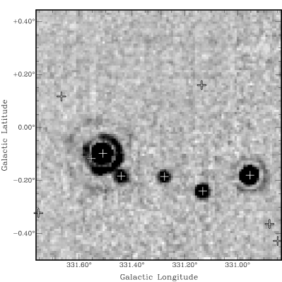
Refer to caption — Figure 1: Water maser emission in one spectral channel at $-$ 89.02 km s^-1. Two strong masers can be seen - G331.51-0.09 (left) and G330.96-0.18 (right) - which both show diffraction rings. Plus symbols indicate the positions of identified water masers. Since the image is only a single channel of the data cube, not all masers are seen in the image, as they do not all emit at this velocity.

In Figure 2, we show an azimuthally averaged histogram for G330.96-0.09. The histogram shows both the inner and outer beam rings. The inner ring occurs at a radius of about 3.8′ and contains approximately 14% of the flux of the main peak. The outer ring occurs at about 8.3′ and contains approximately 3.5% of the flux of the main peak. We estimate the FWHM of the beam from the radial profile to be 2.2′.

Recent observations by Urquhart et al. (2010) of the water masers in Orion-KL have been used to characterise the Mopra radiotelescope. We find that the positions and intensities of the rings, as well as the size of the beam that we derive above agree well with their results.

2.3 Mopra efficiency and stability

We adopt values from Urquhart et al. (2010) for the main beam size (2.2′ at 22.2 GHz), efficiency (0.54 at 22.2 GHz) and Jy K^-1 conversion factor (12.5 at 22.2 GHz).

During the course of the HOPS observations, we regularly performed observations of a number of well known line sources in the sky, including Orion. These observations were typically conducted once each night and consisted of a position-switch with 2 minutes on-source integration. The standard HOPS zoom configuration was used (Table 1). The purpose of these observations is to assess the stability of the telescope system over time and through different observing conditions. Whilst the zoom configuration includes strong maser lines, especially the H₂O maser line, we did not use this line for our calibration as the intensity is known to vary with time (Felli et al., 2007). Instead, we found the strong radio recombination emission lines (H69 $\alpha$ and H62 $\alpha$ ) well suited for calibration, as they are not expected to significantly vary in intensity over the timescale of our observations.

We measure the integrated intensity of the lines by fitting the spectrum with a single gaussian curve and determining the area under that curve, using standard routines in the ASAP software package¹¹1The ATNF Spectral Analysis Package; http://svn.atnf.csiro.au/trac/asap.

Figure 3 shows the distribution of measured integrated intensities for both radio recombination lines throughout the observations. Filled circles indicate integrated intensities for the H69 $\alpha$ line and open squares indicate integrated intensities for the H62 $\alpha$ line. We might expect that if there is significant atmospheric attenuation, then the integrated intesities might be correlated with elevation and/or system temperature. However, Figure 3 shows that the distribution of integrated intensities for each line does not appear to correlate with either elevation or system temperature. But Figure 3 does show a scatter of integrated intensities. We calculate the standard deviation of integrated intensities is 15 per cent for H69 $\alpha$ and 16 per cent for H62 $\alpha$ . Thus, about 95 per cent (two standard deviations) of all integrated intensities are within 30 per cent of the mean integrated intesity. We assign 30 per cent as the uncertainty in the intensities of the HOPS data. Since the radio recombination line emission in Orion is extended, it is possible that the actual uncertainty is less then this as some of the scatter in Figure 3 may be due to small pointing errors of the telescope. Thus we consider 30 per cent as an upper limit.

Figure 3 does show a significant difference in the integrated intensities of the two radio recombination lines, with the H62 $\alpha$ line weaker than the H69 $\alpha$ line, on average. Figure 4 shows the distribution of the ratio of H69 $\alpha$ /H62 $\alpha$ integrated intensities for simultaneous observations. The mean of this distribution is 1.37, with a standard deviation of 0.07. This shows that the ratio of intensities appears stable over time. Therefore, whilst the absolute intensity scale may be uncertain by a factor of 30 per cent, the relative intensity scale of different spectral lines measured using simultaneous observations is likely to be no worse than 5 per cent. We note that the higher intensity of the H69 $\alpha$ line, compared to the H62 $\alpha$ line is most likely because the beam at 19.6 GHz (the H69 $\alpha$ line frequency) is larger than at 26.9 GHz (the H62 $\alpha$ line frequency) and encompassess more extended radio recombination line emission.

3 Survey Design

Previous observations of the Galactic plane in continuum (Schuller et al., 2009), thermal line (Jackson et al., 2006; Dame, Hartmann & Thaddeus, 2001) and methanol maser emission (Walsh et al., 1998; Green et al., 2009) indicate that molecular material is concentrated in a region within about 30^∘ in Galactic longitude of the Galactic centre. The survey region for HOPS was tailored to cover the bulk of this emission, where the nominal survey region covered Galactic longitudes 290 ${}^{\circ}<l<360^{\circ}$ and 0 ${}^{\circ}<l<30^{\circ}$ . The bulk of methanol masers (Walsh et al., 1998; Green et al., 2009) appear to be confined to within half a degree of the Galactic Plane and H₂O and methanol masers are commonly found in the same star forming regions, so the survey covered nominal Galactic latitudes from $-0.5^{\circ}<b<+0.5^{\circ}$ . Our choice of survey region was also based on the amount of observing time that would be reasonably allocated in order to complete the project.

Based on our pilot observations (Walsh et al., 2008), we found the most suitable method was to divide the survey region into blocks of 0.5^∘ by 0.5^∘. Each block was observed twice in the on-the-fly (OTF) mapping mode, scanning once in Galactic longitude and once in Galactic latitude. Adjacent scans were separated by 51″, to give Nyquist sampling of the beam at the highest observing frequency (27.5 GHz). At lower frequencies, the observations consequently oversample the mapped region. The scanning rate was 15″ s^-1 and spectra were stored every 2 seconds, giving a 30″ spacing between spectra in each row. Each block requires about 2 hours of continuous observations to complete. Thus, each square degree of sky requires approximately 8 hours to be fully observed. We calculate that each position was observed for effectively one minute on-source, using this method.

The positions of reference observations for the 0.5^∘ by 0.5^∘ blocks were chosen to typically lie at b=+0.6^∘ or b=-0.6^∘, close to one corner of each block. Each reference position was initially checked for emission with a position switch observation, with 2 minutes on-source integration time. Any potential reference position showing emission was discarded and a new reference position was chosen and checked in the same manner.

In order to minimise variations in sensitivity across the survey region, observations were generally limited to elevations greater than 30^∘, although observations were occasionally made at slightly lower elevations during exceptionally good weather conditions. During good weather and at high elevation, typical system temperatures were 50 K at 19.5 GHz and 65 K at 27.5 GHz. We discarded all data with a system temperature of over 120 K. This upper limit was usually reached when observing through average weather conditions close to an elevation of 30^∘ or during poor weather conditions. We also discarded data where the system temperature varied quickly due to clouds passing through the telescope beam. Such variations were typically 20 K or greater and had the effect of producing striped features in the reduced data.

Pointing observations were conducted at the start of the survey at a variety of positions across the sky. We found that the global pointing model of Mopra was never more than 15 arcseconds from the true position. We estimate that for the majority of HOPS observations the pointing was better than 10 arcseconds, which is less than 10% of the beam width. Consequently, regular pointing updates were not used, in favour of the global pointing model.

4 Data reduction

Data were initially reduced using livedata and gridzilla²²2Developed by Mark Calabretta: http://www.atnf.csiro.au/people/mcalabre/livedata.html, which are both AIPS++ packages written for the Parkes radiotelescope and adapted for Mopra. Livedata performs a bandpass calibration for each row along the scanning direction, using the preceding reference scan. A first order polynomial (ie. a straight line) is fit to the baseline and then subtracted. In order to minimise the effects of noisy channels at the start and end of each zoom window, the first and last 150 channels were masked before performing the baseline fitting.

Gridzilla regrids and combines the data from multiple scanning directions onto a data cube. We chose to regrid onto pixels of 30 $\times$ 30 arcseconds. Data were automatically weighted according to their system temperature and data with system temperatures above 120 K were discarded. Data cubes were then processed in miriad to smooth and/or bin the data, before the creation of peak temperature maps, which were used to find sources of emission. Peak temperature maps are created in miriad, using the “moment=-2” option in the task moment. Peak temperature maps are two-dimensional maps similar to moment zero, (integrated intensity) maps more commonly used in radio astronomy, but each pixel in the two-dimensional peak temperature map corresponds to the highest intensity pixel of the spectrum from the full data cube, at each position on the sky. We found that the peak temperature maps were more sensitive than moment zero maps in detecting weak emission, especially with imperfect baselines and wide bandwidths that were features of the HOPS data.

5 Source finding

We employed a variety of methods to detect H₂O maser emission. These same methods were used to detect other rarer masers (see §7.3). Initially, we smoothed the data with a 90 $\times$ 90 arcsecond two-dimensional Gaussian kernel. We found that this size effectively reduced the noise by about 15%, compared to the maser emission. This kernel is slightly smaller than the size of the beam (132″), however, we found that a smoothing kernel the size of the beam produced maps that were not as sensitive to identifying weak masers close to the noise level.

After smoothing, the data were converted to peak temperature maps. These maps were visually inspected for maser candidates. Masers were initially identified by inspecting the spectrum at the position of a maser candidate in the peak temperature map and looking for a peak that contained at least two adjacent channels where at least one channel was greater than 3 $\times$ the rms noise level and where the sum of all emission channels was greater than 5 $\times$ the rms noise level. These values were chosen as they appear to give the best efficiency for detection of real features, with little contamination. Any weak maser candidates were then followed up with a position-switch observation, with 2 minutes on-source integration time, which typically had rms noise levels a factor of 1.4 better than the original map. Any maser candidate that was not seen in the followup spectrum was considered spurious and discarded.

After identifying masers with the above method, the spatially-smoothed data cube was then spectrally binned (along the velocity axis), with three channels combined into each bin. A new peak temperature map was made from this spatially-smoothed and spectrally-binned map then visually inspected for other masers. This method was used because some masers show line widths significantly greater than the channel width (0.45 km s^-1). Binning the data in this way allows us to pick out weak masers with line widths approximately 1.4 km s^-1. We also binned the data with eight channels per bin, but did not find any new detections over the unbinned and 3-channel binned data.

We note that our method is well suited to finding weak H₂O masers that typically have large enough line widths to appear in more than one channel. However, the method may miss some weak methanol masers, which are known to have very narrow line widths, since the methanol maser may appear in a single channel and be flagged as a noise spike.

5.1 Positional Accuracy

The reported positions of H₂O masers (see §6) are based on the position of the brightest emission pixel in the data cube. Whilst the Mopra beam is 2.2′ at 22.2 GHz, the positions of bright masers should be more accurate than this. Some of the detected H₂O masers have been previously observed with the ATCA (Breen et al., 2010) to higher positional accuracy than our Mopra observations. We can therefore compare the positions of those masers that appear in both surveys. Figure 5 shows the distribution of offsets for the masers we have detected with Mopra, compared to the positions given by Breen et al. (2010). We find that nearly all of our H₂O maser positions are no more than one arcminute offset from the corresponding ATCA position. We also find that the median offset is 20″, indicating that most of the reported positions of masers are probably no more than 20″ off the real positions.

We also note that of the 34 maser sites that overlap with (Breen et al., 2010), 9 (ie. 26 per cent) are identified as multiple sites by (Breen et al., 2010) but are not resolved by the Mopra beam in our observations. We expect that many more maser spectra identified in this work may consist of multiple maser sites.

6 Results

Here we report results on the H₂O maser emission detected in HOPS. Occasional detections of rare masers are reported in §7.3 and results from other thermal spectral lines such as NH₃, radio recombination lines and HCCCN (3–2) will be reported in later papers.

H₂O maser emission was found toward 540 distinct sites in the region observed in HOPS. The properties of these sites are summarised in Table 2. The source name (column 1) is derived from the Galactic coordinates. Columns 2 and 3 list the coordinates of the site. Peak flux density, velocity and FWHM of the strongest maser spot in the spectrum are listed in columns 4, 5 and 6, respectively. The minimum and maximum velocities over which emission has been detected are given in columns 7 and 8, respectively. The last column lists whether a maser is a new detection or previously reported. Reference numbers to previously reported masers in the last column are the first detection of the maser and are given in Table 12. Spectra of the masers are presented in Figure 6. The strongest maser (G27.18 $-$ 0.08) has a peak flux density of 3933 Jy and the weakest maser (G305.56 $+$ 0.01) has a peak flux density of 0.7 Jy. Note that the weakest maser was detected because it shows a broad line FWHM (5.0 km s^-1). The median peak flux density is 11.4 Jy. We detect 62 masers (9%) with peak flux densities over 100 Jy. 334 of the detected H₂O maser sites are new detections (62%). Note that since the Mopra beam for these observations is 2′ it is likely that many of the maser spectra are composed of multiple maser sites, so that 540 maser sites is almost certainly a lower limit.

Table 2: Properties of detected water masers. Column 1 lists the source name, derived from the Galactic coordinates. Right ascension and declination coordinates are given in columns 2 and 3, respectively. Properties of the strongest maser spot are given in columns 4, 5 and 6: column 4 lists the peak flux density, column 5 lists the line centre velocity and column 6 lists the line FWHM of the brightest maser spot. For maser sites with multiple maser spots, the minimum and maximum velocity of the maser spots are given in columns 7 and 8, respectively. Otherwise, for maser sites with only a single maser spot, no velocity range is given. Column 9 lists whether the maser site is a new detection (“NEW”) or a previous detection. Previous detections are listed as numbers which refer to Table 12. If a previous detection also identifies the maser site with an evolved star, this is also noted. If a previously known evolved star is associated with a newly discovered H₂O maser, then ‘NEW’ is written, as well as the reference number for the evolved star association.

Source	RA	Dec	Strongest Maser Spot			Velocity Range		Comments¹
Name	(J2000)	(J2000)	Peak Flux	Velocity	FWHM	Min	Max
	(h m s)	(^∘ ′ ″)	Density (Jy)	(km s^-1)	(km s^-1)	(km s^-1)
G0.05 $-$ 0.22	17 46 35.9	-29 00 15	7.4	12.4	0.8	11.7	14.7	1
G0.31 $-$ 0.18	17 47 01.6	-28 46 00	39.2	10.6	0.8	-6.3	21.4	2
G0.31 $-$ 0.21	17 47 10.3	-28 46 48	6.6	21.5	0.9	10.3	22.4	2
G0.34 $+$ 0.09	17 46 04.0	-28 36 04	36.6	7.1	0.6			1
G0.37 $-$ 0.17	17 47 09.7	-28 42 22	22.4	-9.1	0.9	-9.7	-5.2	1
G0.38 $+$ 0.03	17 46 23.8	-28 35 50	31.8	40.0	1.6	30.3	41.5	3
G0.53 $+$ 0.18	17 46 09.8	-28 23 29	6.8	-1.4	0.7			2
G0.60 $-$ 0.00	17 47 03.2	-28 25 18	7.1	37.2	0.9	18.2	75.7	NEW
G0.67 $-$ 0.04	17 47 20.7	-28 23 13	508.1	70.7	3.8	23.3	127.0	4
G1.01 $-$ 0.24	17 48 56.4	-28 12 06	4.0	3.4	0.7			NEW
G1.05 $-$ 0.07	17 48 21.8	-28 04 46	11.1	-37.1	2.8			NEW
G1.15 $-$ 0.13	17 48 50.0	-28 01 18	177.5	-21.6	1.5	-25.7	-13.0	5
G1.17 $-$ 0.04	17 48 31.0	-27 57 27	35.4	-22.3	1.6			NEW
G2.53 $-$ 0.23	17 52 23.7	-26 53 18	4.2	1.5	0.6			NEW
G2.58 $-$ 0.44	17 53 19.9	-26 56 44	72.6	-6.0	0.8	-25.5	4.8	6
G2.60 $-$ 0.36	17 53 04.9	-26 53 18	9.1	-20.5	2.1	-21.9	-10.9	NEW
G2.90 $-$ 0.43	17 54 01.0	-26 40 12	8.6	82.4	1.0			NEW
G2.93 $+$ 0.28	17 51 22.3	-26 17 16	4.1	-42.8	0.5			NEW
G3.88 $+$ 0.27	17 53 33.6	-25 28 18	4.3	10.3	0.9			NEW
G4.00 $+$ 0.33	17 53 34.9	-25 20 07	3.5	13.6	0.9			NEW
G4.00 $-$ 0.17	17 55 29.5	-25 35 12	2.8	-55.0	7.5			NEW
G4.83 $+$ 0.22	17 55 51.2	-24 40 13	3.2	11.1	2.7			7
G4.89 $-$ 0.13	17 57 19.9	-24 47 41	42.8	6.9	1.4			NEW
G5.37 $+$ 0.05	17 57 41.2	-24 17 33	10.0	2.5	1.1			NEW
G5.52 $-$ 0.25	17 59 09.9	-24 19 01	2.6	21.9	1.4			NEW
G5.63 $-$ 0.29	17 59 34.0	-24 14 38	2.5	17.5	1.2			NEW
G5.66 $+$ 0.42	17 56 57.0	-23 51 36	18.4	18.3	1.0	13.9	19.7	NEW
G5.71 $-$ 0.50	18 00 31.9	-24 16 28	4.2	12.3	0.9			NEW, 8 - Mira Variable
G5.88 $-$ 0.39	18 00 29.8	-24 04 06	207.7	9.4	0.9	2.4	11.8	9
G5.90 $-$ 0.43	18 00 41.6	-24 04 28	7.4	10.1	2.7	7.5	47.0	2
G5.91 $-$ 0.39	18 00 33.1	-24 02 48	43.0	-61.5	2.2	-64.7	-52.6	2
G6.09 $-$ 0.12	17 59 54.9	-23 45 34	6.8	3.0	0.7			10
G6.19 $-$ 0.36	18 01 02.7	-23 47 11	5.9	-29.3	0.8			NEW
G6.20 $-$ 0.01	17 59 43.4	-23 36 02	2.8	-35.1	4.9	-38.3	-30.4	NEW
G6.23 $-$ 0.06	17 59 59.5	-23 36 21	4.8	16.9	0.9			NEW
G6.23 $+$ 0.32	17 58 34.7	-23 24 54	11.9	18.1	1.2	2.4	87.2	NEW
G6.59 $-$ 0.19	18 01 16.1	-23 21 22	4.6	-2.0	1.0			NEW
G6.61 $-$ 0.08	18 00 54.7	-23 16 54	29.1	5.3	1.0	-0.7	7.5	2
G6.79 $-$ 0.26	18 01 58.9	-23 12 57	7.8	11.7	0.8	5.5	13.2	2
G6.92 $-$ 0.23	18 02 06.2	-23 05 21	8.8	-10.0	3.3	-14.0	-4.8	11
G7.38 $-$ 0.09	18 02 34.7	-22 37 24	7.6	42.4	1.0			NEW
G7.46 $-$ 0.28	18 03 27.3	-22 38 29	3.7	23.7	1.8			NEW
G7.47 $+$ 0.05	18 02 14.1	-22 28 09	42.4	-16.3	1.6	-87.5	-10.3	NEW
G7.54 $-$ 0.06	18 02 48.5	-22 27 38	4.4	-1.1	3.2			NEW
G8.00 $-$ 0.27	18 04 34.3	-22 09 57	12.1	36.1	0.8	25.3	43.9	NEW
G8.08 $+$ 0.15	18 03 11.2	-21 53 30	7.8	22.1	1.1			NEW
G8.20 $+$ 0.13	18 03 29.2	-21 47 56	10.7	18.4	1.0	0.4	19.6	NEW
G8.32 $-$ 0.10	18 04 38.0	-21 48 28	4.1	36.9	2.4			NEW
G8.41 $-$ 0.30	18 05 33.7	-21 49 49	10.3	47.6	1.2			NEW
G8.63 $-$ 0.24	18 05 48.4	-21 36 07	8.0	1.3	1.0			NEW

¹“NEW” indicates a newly detected maser, otherwise a number (refer to Table 12) is given for a previous detection. The majority of masers are presumed to be associated with star formation. Previously known associations with evolved stars are referenced, but we await higher precision positions to associate the majority of masers.

Table 3: continued

… Source RA Dec Strongest Maser Spot Velocity Range Comments¹ Name (J2000) (J2000) Peak Flux Velocity FWHM Min Max (h m s) (^∘ ′ ″) Density (Jy) (km s^-1) (km s^-1) (km s^-1) G8.67 $-$ 0.36 18 06 19.7 -21 37 30 29.8 24.7 0.7 -5.5 44.8 12 G8.70 $-$ 0.43 18 06 38.5 -21 37 57 4.9 32.8 1.3 NEW G8.73 $-$ 0.39 18 06 34.2 -21 35 40 6.0 46.7 0.7 30.4 47.4 NEW G8.83 $-$ 0.03 18 05 25.7 -21 19 24 38.9 -9.5 1.7 -13.3 -7.2 7 G8.93 $-$ 0.02 18 05 35.6 -21 13 44 88.9 7.0 0.9 5.7 49.2 13 - M supergiant G9.10 $-$ 0.40 18 07 22.8 -21 16 14 18.3 62.9 1.2 -62.0 289.3 14 - water fountain G9.62 $+$ 0.19 18 06 15.0 -20 31 43 60.2 5.6 1.7 -9.8 9.1 15 G9.95 $+$ 0.46 18 05 57.2 -20 06 38 2.9 -65.8 1.1 -66.5 -61.9 NEW G9.98 $-$ 0.03 18 07 51.0 -20 19 15 13.4 45.2 1.7 43.7 59.6 7 G10.34 $-$ 0.14 18 08 59.0 -20 03 58 19.9 19.2 1.1 5.8 35.7 16 G10.39 $-$ 0.01 18 08 35.3 -19 57 26 7.2 45.9 1.2 NEW G10.44 $-$ 0.01 18 08 42.5 -19 54 24 19.7 70.4 1.8 67.8 83.8 2 G10.48 $+$ 0.03 18 08 37.4 -19 51 28 108.3 70.7 1.1 40.7 88.1 17 G10.62 $-$ 0.38 18 10 26.1 -19 55 52 381.5 0.3 3.1 -19.4 8.8 18 G10.64 $-$ 0.50 18 10 56.1 -19 58 35 59.7 -67.9 3.9 -71.8 -46.1 NEW G10.89 $+$ 0.13 18 09 07.4 -19 27 20 13.8 23.9 2.2 9.0 26.0 NEW G10.96 $+$ 0.03 18 09 38.9 -19 26 18 25.7 24.3 0.5 19 G11.65 $-$ 0.06 18 11 22.2 -18 52 28 1.4 3.7 6.1 -3.1 30.8 NEW G11.73 $-$ 0.18 18 11 57.2 -18 51 53 5.9 -43.0 0.9 NEW G11.87 $+$ 0.00 18 11 35.6 -18 39 21 21.6 21.2 0.9 20.2 38.9 NEW G11.92 $-$ 0.14 18 12 13.2 -18 40 49 7.1 33.8 0.8 23.8 49.6 12 G11.96 $-$ 0.16 18 12 22.0 -18 39 09 6.2 40.3 1.4 38.5 45.2 NEW G12.22 $-$ 0.09 18 12 38.5 -18 23 39 3.2 20.8 4.6 4 G12.22 $+$ 0.38 18 10 53.2 -18 09 56 20.9 37.7 0.9 NEW G12.22 $-$ 0.33 18 13 31.4 -18 29 57 21.5 -15.8 1.3 NEW G12.55 $-$ 0.18 18 13 39.2 -18 08 45 9.4 59.5 0.8 NEW G12.68 $-$ 0.18 18 13 53.5 -18 01 31 163.4 58.6 0.8 53.7 61.9 20 G12.82 $-$ 0.19 18 14 13.3 -17 54 55 2.8 36.1 1.2 30.5 37.4 4 G12.91 $-$ 0.02 18 13 45.5 -17 45 06 19.4 13.6 2.3 4 G12.92 $-$ 0.24 18 14 36.4 -17 51 05 5.5 35.6 1.6 28.9 36.3 4 G12.94 $-$ 0.04 18 13 55.1 -17 44 02 6.1 20.9 0.7 NEW G12.94 $-$ 0.07 18 14 00.7 -17 44 45 57.0 33.5 0.7 NEW G13.19 $+$ 0.06 18 14 03.2 -17 27 56 9.1 -4.1 3.5 4 G13.44 $+$ 0.24 18 13 52.9 -17 09 31 9.0 48.2 0.9 40.7 55.4 NEW G13.46 $+$ 0.22 18 14 00.4 -17 09 23 7.1 16.4 1.1 NEW G13.69 $-$ 0.05 18 15 26.9 -17 04 39 31.9 44.7 0.9 NEW G13.82 $+$ 0.27 18 14 32.0 -16 48 58 2.9 70.9 1.3 NEW G13.88 $+$ 0.29 18 14 34.8 -16 44 50 20.0 -41.7 1.4 -45.6 -14.0 4 G14.03 $-$ 0.31 18 17 04.6 -16 54 01 5.9 129 1.0 NEW G14.11 $+$ 0.09 18 15 45.3 -16 38 38 47.9 9.2 0.8 21 G14.17 $-$ 0.05 18 16 23.6 -16 39 35 126.5 54.3 1.3 35.1 57.9 8 G14.20 $-$ 0.18 18 16 56.9 -16 41 38 27.5 24.1 1.3 NEW G14.61 $+$ 0.03 18 16 59.6 -16 14 10 21.9 29.8 0.9 7.6 32.0 21 G14.68 $-$ 0.05 18 17 24.2 -16 12 47 13.0 -5.2 0.8 -6.7 -0.9 NEW G14.78 $-$ 0.36 18 18 43.9 -16 16 16 4.9 31.6 1.3 30.0 34.0 NEW G15.09 $+$ 0.21 18 17 16.5 -15 43 22 21.4 28.0 0.9 20.7 32.1 22 G15.54 $-$ 0.13 18 19 22.3 -15 29 28 4.3 23.1 0.6 NEW G15.55 $+$ 0.37 18 17 36.7 -15 14 38 2.0 70.1 2.9 NEW G15.97 $+$ 0.24 18 18 53.2 -14 56 09 49.5 58.3 0.6 -98.1 190.5 NEW G16.05 $-$ 0.13 18 20 24.7 -15 02 24 13.7 62.2 0.6 NEW G16.25 $+$ 0.19 18 19 37.0 -14 42 38 3.7 -1.3 1.7 NEW G16.28 $+$ 0.42 18 18 50.7 -14 34 55 1.0 -84.7 3.8 NEW G16.46 $+$ 0.44 18 19 06.7 -14 24 32 18.2 21.2 1.5 18.0 46.7 NEW G16.58 $-$ 0.04 18 21 07.1 -14 31 38 63.2 63.9 1.3 56.5 69.5 12 G17.55 $-$ 0.12 18 23 15.8 -13 42 35 477.2 30.6 1.1 28.7 57.2 13 G17.64 $+$ 0.17 18 22 24.5 -13 29 42 126.7 26.0 1.0 15.7 27.3 23 G17.97 $+$ 0.09 18 23 18.5 -13 14 36 8.3 26.6 0.8 NEW G17.98 $+$ 0.24 18 22 47.8 -13 09 27 15.0 15.4 0.9 22 G18.16 $+$ 0.39 18 22 36.8 -12 56 14 10.4 55.6 0.9 NEW G18.24 $-$ 0.12 18 24 35.2 -13 05 53 8.4 39.1 1.8 NEW G18.52 $+$ 0.15 18 24 09.9 -12 43 25 3.0 22.4 3.0 NEW

Table 4: continued

… Source RA Dec Strongest Maser Spot Velocity Range Comments¹ Name (J2000) (J2000) Peak Flux Velocity FWHM Min Max (h m s) (^∘ ′ ″) Density (Jy) (km s^-1) (km s^-1) (km s^-1) G18.55 $+$ 0.04 18 24 38.0 -12 45 21 10.7 32.2 0.5 31.3 35.2 NEW G18.61 $-$ 0.08 18 25 10.3 -12 45 30 6.0 41.3 1.2 40.0 52.4 NEW G18.73 $-$ 0.22 18 25 55.3 -12 42 49 28.5 36.7 1.3 32.2 46.3 NEW G18.88 $-$ 0.47 18 27 07.0 -12 41 55 7.7 65.1 1.5 NEW G19.00 $-$ 0.23 18 26 27.8 -12 28 57 21.8 -15.9 7.2 NEW G19.15 $-$ 0.47 18 27 36.4 -12 27 23 41.0 30.2 0.7 22.1 37.3 NEW, 24 - M supergiant G19.27 $+$ 0.09 18 25 48.3 -12 05 25 3.4 28.6 1.9 NEW G19.47 $+$ 0.18 18 25 53.3 -11 52 26 5.0 -6.7 2.3 -12.6 20.7 NEW G19.49 $+$ 0.16 18 25 58.7 -11 52 14 4.5 27.0 1.1 22.4 28.3 NEW G19.61 $-$ 0.23 18 27 37.9 -11 56 32 127.4 41.9 3.4 23.0 57.9 25 G19.71 $-$ 0.26 18 27 54.7 -11 51 55 6.4 38.9 1.0 38.1 44.1 NEW G20.08 $-$ 0.13 18 28 10.3 -11 28 39 19.7 46.4 0.8 37.5 47.4 12 G20.78 $-$ 0.06 18 29 12.7 -10 49 47 37.8 59.2 1.8 26 G21.04 $-$ 0.06 18 29 42.9 -10 35 36 5.4 35.6 1.5 27 G21.80 $-$ 0.12 18 31 21.3 -09 56 56 83.2 106.2 2.1 -53.1 164.7 28 - Water Fountain G21.81 $+$ 0.15 18 30 24.6 -09 49 02 7.3 2.7 4.3 -4.7 10.9 NEW, 29 - Carbon Star G21.88 $+$ 0.02 18 31 01.8 -09 48 44 17.3 21.4 3.2 18.9 26.2 15 G21.95 $+$ 0.01 18 31 11.3 -09 45 25 14.6 109.8 0.8 95.6 111.5 23 G22.00 $+$ 0.07 18 31 03.0 -09 41 10 10.0 147.2 2.3 145.4 152.1 NEW, 30 - OH/IR star G22.03 $+$ 0.22 18 30 34.3 -09 35 39 12.7 53.7 0.7 31 G22.82 $-$ 0.17 18 33 26.8 -09 04 10 7.9 41.0 1.2 NEW G22.97 $-$ 0.37 18 34 27.1 -09 01 54 3.3 74.8 2.0 NEW G23.00 $-$ 0.41 18 34 38.7 -09 01 05 167.8 68.9 1.3 62.3 82.6 31 G23.15 $-$ 0.23 18 34 16.8 -08 48 09 19.8 110.2 0.9 108.8 113.3 NEW G23.21 $-$ 0.38 18 34 55.7 -08 49 12 13.8 79.4 1.2 77.1 143.5 31 G23.41 $-$ 0.21 18 34 42.3 -08 33 58 5.0 102.5 1.5 100.8 135.8 32 G23.46 $-$ 0.35 18 35 18.2 -08 35 12 4.1 105.6 2.3 NEW G23.48 $+$ 0.10 18 33 44.1 -08 21 26 10.5 87.0 2.5 49.2 89.5 NEW G23.91 $+$ 0.08 18 34 35.2 -07 59 16 3.7 73.1 4.2 71.3 97.9 19 G23.98 $+$ 0.15 18 34 26.6 -07 53 38 13.8 31.5 1.6 33 G23.98 $+$ 0.24 18 34 08.1 -07 50 43 11.3 99.8 1.2 94.5 107.6 NEW G24.33 $+$ 0.14 18 35 08.3 -07 35 16 16.3 110.9 1.4 31 G24.43 $+$ 0.09 18 35 30.2 -07 31 19 3.7 111.9 1.4 NEW G24.45 $+$ 0.26 18 34 57.3 -07 25 24 10.7 113.9 0.5 NEW G24.46 $+$ 0.20 18 35 10.7 -07 26 35 34.0 120.7 1.9 115.7 122.6 NEW G24.50 $-$ 0.03 18 36 05.3 -07 30 50 20.1 111.3 0.8 73.7 153.0 13 G24.79 $+$ 0.08 18 36 12.9 -07 12 04 226.7 111.2 2.4 89.5 116.4 18 G24.94 $-$ 0.03 18 36 54.5 -07 07 17 10.5 -4.9 1.3 NEW G24.94 $+$ 0.08 18 36 31.3 -07 04 18 280.0 42.9 0.6 31 G24.99 $-$ 0.17 18 37 29.7 -07 08 25 7.5 96.4 1.1 NEW G25.06 $+$ 0.27 18 36 02.3 -06 52 44 9.1 77.6 2.2 NEW, 34 - OH/IR star G25.11 $-$ 0.03 18 37 13.1 -06 58 27 7.5 101.2 2.2 93.8 109.1 NEW G25.29 $-$ 0.04 18 37 35.3 -06 48 52 4.6 114.7 1.4 105.7 119.3 NEW G25.38 $-$ 0.18 18 38 15.9 -06 47 56 111.8 68.6 1.0 35 G25.40 $+$ 0.03 18 37 31.2 -06 41 03 26.1 -15.9 0.7 22 G25.52 $-$ 0.11 18 38 14.6 -06 38 43 9.1 98.8 0.7 NEW G25.73 $-$ 0.11 18 38 37.7 -06 27 38 13.0 97.4 1.3 96.5 105.9 NEW G25.82 $-$ 0.05 18 38 35.2 -06 21 06 20.6 125.7 0.7 82.3 127.4 NEW G25.83 $-$ 0.18 18 39 02.9 -06 24 07 295.0 90.6 2.6 82.8 97.3 31 G25.91 $-$ 0.08 18 38 50.7 -06 16 56 14.1 108.6 0.7 102.9 126.2 NEW G25.98 $-$ 0.08 18 39 00.0 -06 13 05 11.6 90.0 1.5 NEW G26.11 $-$ 0.09 18 39 16.7 -06 06 38 64.2 23.5 1.4 22.1 27.4 22 G26.13 $-$ 0.03 18 39 06.1 -06 04 08 11.1 84.9 3.0 72.7 101.3 NEW G26.40 $-$ 0.10 18 39 50.7 -05 51 17 5.8 98.6 2.8 78.0 101.9 NEW G26.51 $+$ 0.28 18 38 40.7 -05 34 53 52.4 103.3 3.6 101.0 108.3 7 G26.53 $+$ 0.40 18 38 17.4 -05 30 49 11.3 100.9 0.9 NEW G26.55 $-$ 0.29 18 40 47.6 -05 48 56 11.5 111.6 3.5 105.0 117.1 NEW G26.85 $+$ 0.16 18 39 44.3 -05 20 34 3.3 97.0 1.2 83.0 111.6 NEW G27.01 $-$ 0.03 18 40 42.6 -05 17 02 6.3 -15.2 0.9 -19.1 -14.0 NEW G27.08 $+$ 0.20 18 40 01.6 -05 06 43 1.0 27.8 13.3 NEW G27.18 $-$ 0.08 18 41 11.6 -05 08 53 3932.7 17.5 0.9 13.2 33.6 36

Table 5: continued

… Source RA Dec Strongest Maser Spot Velocity Range Comments¹ Name (J2000) (J2000) Peak Flux Velocity FWHM Min Max (h m s) (^∘ ′ ″) Density (Jy) (km s^-1) (km s^-1) (km s^-1) G27.33 $+$ 0.18 18 40 33.7 -04 54 30 20.0 33.9 0.9 33.1 38.4 NEW, 29 - Carbon Star G27.37 $-$ 0.16 18 41 49.6 -05 01 24 25.6 88.2 2.2 86.1 98.9 31 G27.41 $-$ 0.05 18 41 31.1 -04 56 12 5.0 108.7 2.0 100.9 109.9 NEW G27.50 $-$ 0.28 18 42 31.1 -04 57 44 2.9 -15.4 1.3 -39.6 -11.2 NEW G27.60 $+$ 0.08 18 41 23.7 -04 42 21 4.1 35.4 0.9 23.4 41.6 NEW G27.70 $+$ 0.20 18 41 09.7 -04 33 48 2.4 62.1 5.3 NEW G27.78 $+$ 0.06 18 41 49.3 -04 33 14 8.3 98.4 1.2 92.4 109.6 31 G27.87 $-$ 0.23 18 43 00.8 -04 36 47 21.0 12.3 0.7 19 G27.93 $+$ 0.24 18 41 25.5 -04 20 39 58.1 62.4 1.3 35.4 65.9 37 G28.01 $-$ 0.43 18 43 57.2 -04 34 38 18.0 19.3 0.6 NEW G28.21 $-$ 0.05 18 42 58.9 -04 13 40 23.7 95.4 1.1 NEW G28.34 $+$ 0.14 18 42 32.4 -04 01 18 41.3 17.5 2.0 NEW G28.40 $+$ 0.08 18 42 51.4 -03 59 50 201.1 77.7 0.7 76.9 86.1 31 G28.41 $+$ 0.07 18 42 55.8 -03 59 47 26.6 34.5 0.9 21.4 40.3 31 G28.62 $+$ 0.06 18 43 21.5 -03 48 31 37.7 -3.9 0.7 NEW G28.65 $+$ 0.03 18 43 29.6 -03 47 52 8.7 103.8 0.8 NEW G28.79 $+$ 0.24 18 43 00.5 -03 34 33 3.0 108.6 5.1 35 G28.81 $+$ 0.37 18 42 36.5 -03 29 47 18.6 88.3 0.8 83.5 89.3 31 G28.85 $+$ 0.50 18 42 12.6 -03 24 37 6.3 86.6 4.2 84.2 91.3 31 G28.86 $+$ 0.07 18 43 46.2 -03 35 21 194.5 105.8 3.0 102.3 107.8 15 G28.88 $-$ 0.03 18 44 07.9 -03 36 55 5.7 114.9 1.7 101.8 123.8 19 G28.96 $+$ 0.40 18 42 46.0 -03 20 53 6.2 18.6 2.2 NEW G29.25 $-$ 0.24 18 45 34.8 -03 23 10 5.9 106.0 1.8 98.1 120.9 NEW G29.28 $-$ 0.13 18 45 13.6 -03 18 13 6.5 40.8 0.7 39.5 52.4 NEW G29.33 $-$ 0.16 18 45 25.3 -03 16 53 39.6 47.6 0.9 NEW G29.49 $+$ 0.19 18 44 29.1 -02 58 45 4.9 35.4 2.1 31.5 37.9 NEW G29.92 $-$ 0.04 18 46 05.1 -02 42 08 36.3 40.5 2.1 15.5 42.5 32 G29.96 $-$ 0.01 18 46 02.6 -02 38 59 73.5 99.2 2.1 88.5 110.3 4 G29.98 $+$ 0.12 18 45 38.7 -02 34 13 7.8 102.8 1.1 101.7 122.7 NEW G291.37 $-$ 0.21 11 14 08.3 -60 52 34 79.0 3.0 0.5 NEW G291.58 $-$ 0.42 11 15 05.2 -61 09 11 343.4 0.7 0.9 -8.5 19.3 38 G291.79 $+$ 0.39 11 19 07.9 -60 28 04 7.3 -152.5 0.6 NEW G292.58 $-$ 0.29 11 23 17.2 -61 22 18 12.4 -14.0 3.1 NEW G293.59 $-$ 0.20 11 31 35.6 -61 36 55 17.2 29.4 0.7 NEW G295.09 $-$ 0.46 11 43 12.9 -62 17 09 11.1 25.1 1.3 23.9 27.0 NEW G297.86 $-$ 0.27 12 07 00.2 -62 41 59 13.1 -19.7 2.0 -20.9 2.5 NEW G298.20 $-$ 0.34 12 09 48.4 -62 49 47 3.6 81.0 1.5 NEW G298.22 $-$ 0.33 12 09 57.4 -62 49 28 3.2 36.7 1.2 33.1 38.7 39 G298.23 $-$ 0.38 12 09 57.9 -62 52 31 13.4 40.4 1.1 29.6 41.3 NEW G298.63 $-$ 0.36 12 13 32.2 -62 54 47 30.4 40.0 1.5 39.2 44.3 NEW G298.72 $-$ 0.08 12 14 36.2 -62 39 11 34.7 18.1 1.3 NEW G298.88 $+$ 0.32 12 16 30.9 -62 16 48 26.7 18.4 2.1 9.5 21.1 NEW G299.00 $+$ 0.13 12 17 17.6 -62 29 09 115.2 19.3 0.8 -12.3 29.8 39 G300.32 $-$ 0.27 12 28 24.3 -63 01 12 54.0 33.7 0.8 NEW G300.50 $-$ 0.17 12 30 01.1 -62 56 41 241.4 11.0 1.1 -9.0 12.6 38 G301.13 $-$ 0.22 12 35 32.9 -63 02 21 834.1 -45.8 0.8 -66.8 -28.4 38 G301.35 $+$ 0.02 12 37 32.9 -62 48 40 4.9 -26.8 0.8 NEW G301.76 $+$ 0.29 12 41 13.2 -62 33 23 15.6 -43.7 1.0 -61.5 -19.4 NEW G302.48 $-$ 0.03 12 47 28.7 -62 54 09 25.0 -30.9 0.7 -61.4 6.9 NEW G303.70 $-$ 0.41 12 58 18.3 -63 16 14 17.1 -54.6 1.0 -62.0 -40.2 NEW G303.87 $+$ 0.47 12 59 33.7 -62 23 31 3.5 -63.8 1.3 NEW G304.06 $+$ 0.44 13 01 09.5 -62 24 56 10.7 -51.1 1.5 -52.8 -41.4 NEW G304.07 $+$ 0.41 13 01 18.3 -62 26 24 18.4 -50.5 0.9 NEW G304.37 $-$ 0.34 13 04 09.3 -63 10 31 16.6 29.0 0.8 NEW G305.01 $+$ 0.43 13 09 21.7 -62 22 28 12.1 -54.5 1.0 NEW G305.14 $+$ 0.07 13 10 41.9 -62 43 02 4.2 -38.4 0.8 40 G305.19 $-$ 0.00 13 11 13.7 -62 47 20 25.8 33.4 1.7 -47.5 36.6 38 G305.21 $+$ 0.21 13 11 11.9 -62 34 36 180.0 -39.1 0.8 -47.8 -29.7 41 G305.27 $-$ 0.00 13 11 52.3 -62 46 52 2.4 -37.9 1.5 -39.1 -32.5 40 G305.32 $+$ 0.07 13 12 16.8 -62 42 08 903.4 -45.1 0.7 -45.7 -29.0 40

Table 6: continued

… Source RA Dec Strongest Maser Spot Velocity Range Comments¹ Name (J2000) (J2000) Peak Flux Velocity FWHM Min Max (h m s) (^∘ ′ ″) Density (Jy) (km s^-1) (km s^-1) (km s^-1) G305.36 $+$ 0.15 13 12 34.3 -62 37 13 457.6 -35.6 3.0 -46.3 -29.7 42 G305.36 $+$ 0.21 13 12 33.8 -62 33 33 170.9 -33.6 1.2 -90.5 52.7 43 G305.56 $+$ 0.01 13 14 24.4 -62 44 48 0.7 -37.7 5.0 40 G305.66 $-$ 0.10 13 15 24.1 -62 50 52 6.7 -68.9 1.8 44 G305.73 $+$ 0.08 13 15 49.4 -62 39 19 4.1 -43.9 3.8 40 G305.80 $-$ 0.24 13 16 40.8 -62 58 24 3023.5 -27.6 0.5 -43.2 -24.3 38 G305.82 $-$ 0.12 13 16 44.8 -62 50 42 4.0 -27.5 0.6 -55.9 -15.6 44 G305.83 $-$ 0.08 13 16 51.4 -62 48 31 41.2 -114.5 4.3 -120.1 -83.8 44 G305.89 $+$ 0.02 13 17 14.4 -62 42 21 41.2 -28.3 1.4 -40.4 -26.5 44 G305.95 $+$ 0.03 13 17 46.8 -62 41 26 3.7 -41.5 1.0 44,45 - AGB Star G307.13 $+$ 0.32 13 27 38.3 -62 15 30 87.2 -42.8 0.8 NEW G307.27 $+$ 0.08 13 29 05.3 -62 28 17 3.9 -31.0 1.7 NEW G307.34 $+$ 0.18 13 29 36.4 -62 21 52 2.8 -93.8 5.3 NEW G307.80 $-$ 0.45 13 34 24.6 -62 55 08 47.4 -13.0 1.0 NEW G307.95 $+$ 0.03 13 35 00.0 -62 25 18 3.3 -45.0 5.4 NEW G308.05 $-$ 0.38 13 36 27.8 -62 48 24 8.0 -12.3 0.7 -17.5 -5.8 NEW G308.08 $-$ 0.42 13 36 43.7 -62 50 01 5.1 -16.3 1.2 -17.7 -8.1 NEW G308.13 $-$ 0.30 13 37 01.1 -62 42 21 36.1 0.6 0.7 NEW G308.16 $-$ 0.45 13 37 29.9 -62 51 13 4.4 5.2 3.1 NEW G308.61 $-$ 0.18 13 40 55.9 -62 30 25 2.9 -12.6 3.5 NEW G308.70 $-$ 0.00 13 41 23.3 -62 18 48 2.1 -66.3 1.3 NEW G308.92 $+$ 0.12 13 43 03.4 -62 09 08 3.7 -50.5 1.0 39 G309.29 $-$ 0.47 13 47 11.3 -62 38 49 5.2 -5.8 2.4 NEW G309.38 $-$ 0.13 13 47 20.8 -62 18 07 8.5 -50.6 0.8 38 G309.90 $+$ 0.33 13 50 48.5 -61 43 59 6.9 -54.3 0.8 -55.1 -47.0 NEW G310.34 $-$ 0.07 13 55 15.2 -62 00 58 6.0 -3.5 3.4 NEW G310.52 $-$ 0.22 13 57 03.4 -62 07 12 4.5 55.3 2.3 47.1 58.8 NEW G310.58 $+$ 0.38 13 56 19.0 -61 31 45 5.7 -30.8 0.9 -57.4 -28.1 37 G310.88 $+$ 0.01 13 59 28.4 -61 48 33 15.4 -70.8 1.8 -82.0 -44.2 NEW G311.23 $-$ 0.03 14 02 29.7 -61 45 15 162.2 28.0 1.1 16.1 43.4 44 G311.56 $+$ 0.23 14 04 30.2 -61 24 29 13.3 9.6 2.0 -1.1 12.6 NEW G311.64 $-$ 0.38 14 06 38.9 -61 58 35 215.5 32.2 2.2 14.6 52.9 38 G311.72 $+$ 0.24 14 05 45.1 -61 21 21 108.1 -72.7 1.0 -80.3 -44.5 NEW G312.07 $+$ 0.09 14 08 54.7 -61 23 53 15.0 -32.8 1.7 -38.1 5.6 44 G312.11 $+$ 0.01 14 09 27.1 -61 27 54 11.4 -41.8 1.6 -46.5 -27.6 44 G312.48 $-$ 0.33 14 13 15.4 -61 40 46 11.7 -31.6 3.4 -43.3 -27.3 NEW G313.46 $+$ 0.07 14 19 55.3 -60 58 43 11.5 1.3 1.0 NEW G313.47 $+$ 0.20 14 19 38.8 -60 51 28 14.0 -9.7 0.7 -12.2 1.4 38 G313.57 $+$ 0.32 14 20 04.5 -60 42 23 12.1 -45.2 0.8 -49.0 -39.8 2 G314.23 $+$ 0.26 14 25 17.8 -60 32 29 6.4 -61.4 1.2 NEW G314.33 $+$ 0.11 14 26 29.6 -60 38 45 9.8 -41.8 1.2 2 G314.41 $+$ 0.05 14 27 17.8 -60 40 12 152.5 -43.8 0.5 NEW G314.98 $+$ 0.03 14 31 38.3 -60 28 36 6.3 -54.1 2.2 NEW G315.22 $-$ 0.25 14 34 20.2 -60 38 45 6.4 -64.5 2.0 NEW G315.23 $-$ 0.11 14 33 57.3 -60 30 45 5.8 -16.2 5.6 NEW G315.93 $+$ 0.05 14 38 42.8 -60 05 15 13.6 -7.1 1.1 NEW G316.09 $-$ 0.07 14 40 14.5 -60 07 41 6.7 -53.0 0.9 NEW G316.35 $-$ 0.37 14 43 07.8 -60 17 43 6.8 1.5 2.4 -14.6 5.7 36 G316.40 $-$ 0.32 14 43 19.7 -60 13 44 8.3 -11.5 1.5 -18.1 3.2 38 G316.63 $-$ 0.09 14 44 16.6 -59 55 35 13.6 -21.1 2.9 -24.5 -5.6 9 G316.76 $-$ 0.02 14 44 55.6 -59 48 21 39.9 -34.9 1.6 -53.2 -32.8 9 G316.81 $-$ 0.06 14 45 25.5 -59 49 18 311.0 -47.2 1.6 -52.3 -25.7 41 G317.87 $+$ 0.14 14 52 14.5 -59 10 49 5.1 -3.3 1.0 -4.2 0.7 NEW G317.87 $-$ 0.15 14 53 16.2 -59 26 28 18.0 -52.7 1.2 -54.4 -41.4 NEW G317.98 $+$ 0.12 14 53 08.7 -59 09 00 4.3 -59.1 0.9 -60.3 -44.5 NEW G318.05 $+$ 0.09 14 53 41.7 -59 08 36 805.3 -52.0 3.0 -61.0 -38.3 46 G318.78 $-$ 0.13 14 59 30.6 -59 00 28 731.0 -135.7 2.7 -144.9 -39.1 NEW G318.94 $-$ 0.18 15 00 50.1 -58 58 21 3.7 -33.8 1.4 -38.5 -32.7 38 G319.34 $-$ 0.32 15 04 04.7 -58 54 13 7.2 -36.0 1.4 -40.7 -34.9 NEW G319.39 $-$ 0.01 15 03 13.6 -58 36 13 11.0 -6.4 0.5 -8.9 -0.8 2

Table 7: continued

… Source RA Dec Strongest Maser Spot Velocity Range Comments¹ Name (J2000) (J2000) Peak Flux Velocity FWHM Min Max (h m s) (^∘ ′ ″) Density (Jy) (km s^-1) (km s^-1) (km s^-1) G319.83 $-$ 0.19 15 06 52.2 -58 32 47 16.0 -12.1 2.9 -15.6 -0.5 38 G320.23 $-$ 0.28 15 09 52.8 -58 25 31 5.7 -61.7 1.3 -67.5 -58.9 38 G320.24 $-$ 0.08 15 09 09.8 -58 14 55 3.7 -9.9 1.1 NEW G320.26 $-$ 0.30 15 10 06.6 -58 25 38 7.0 -116.3 2.5 -127.9 -108.4 38 G320.34 $-$ 0.20 15 10 16.2 -58 17 57 23.8 -107.7 1.3 -118.3 -102.3 NEW G320.43 $+$ 0.10 15 09 40.1 -57 59 52 12.3 -10.4 1.0 -16.6 -3.1 NEW G320.90 $-$ 0.29 15 14 15.9 -58 05 25 172.0 -35.9 1.6 -39.9 -33.2 47 G321.04 $-$ 0.50 15 15 58.6 -58 11 41 12.0 -52.4 1.0 -67.3 -51.3 2 G321.38 $-$ 0.29 15 17 22.5 -57 50 20 3.2 -53.9 0.7 -60.0 47.7 NEW G321.93 $-$ 0.00 15 19 41.1 -57 17 55 16.3 -38.6 2.2 -41.3 -34.5 NEW G323.74 $-$ 0.26 15 31 45.0 -56 30 33 11.3 -49.6 1.7 -52.7 -47.8 38 G324.18 $+$ 0.41 15 31 36.1 -55 42 35 11.7 -56.6 1.1 NEW G324.20 $+$ 0.13 15 32 51.8 -55 55 57 82.9 -76.7 1.5 -91.8 -65.4 9 G325.63 $+$ 0.29 15 40 20.8 -54 57 17 21.9 14.8 0.9 NEW G326.06 $-$ 0.14 15 44 32.5 -55 02 41 6.8 -75.0 2.6 -81.1 -70.4 NEW G326.45 $+$ 0.33 15 44 41.1 -54 25 45 6.2 -71.6 0.6 NEW G326.48 $-$ 0.37 15 47 48.0 -54 57 57 4.9 -51.6 1.0 NEW G326.48 $+$ 0.38 15 44 38.6 -54 22 50 67.9 -82.4 0.9 -85.7 -81.3 NEW, 48 - AGB star G326.56 $+$ 0.07 15 46 24.0 -54 34 21 10.3 1.9 1.0 NEW G326.78 $-$ 0.23 15 48 53.9 -54 40 11 93.9 -66.7 0.8 -70.9 -63.0 2 G327.40 $+$ 0.45 15 49 17.7 -53 45 06 135.0 -80.2 1.0 -85.0 -75.8 9 G327.41 $-$ 0.07 15 51 32.1 -54 08 56 9.3 -70.8 2.0 -95.5 -65.9 NEW, 30 - OH/IR star G327.59 $-$ 0.38 15 53 50.8 -54 16 18 24.3 -71.7 1.9 NEW G327.65 $-$ 0.38 15 54 09.2 -54 14 05 9.7 -73.1 2.2 NEW G328.26 $-$ 0.41 15 57 28.3 -53 52 10 11.9 -39.7 1.1 NEW G328.31 $+$ 0.43 15 54 06.1 -53 11 31 138.3 -94.7 1.1 9 G328.94 $-$ 0.12 15 59 42.0 -53 12 18 5.5 -41.3 3.2 NEW G328.99 $-$ 0.43 16 01 20.5 -53 24 39 80.4 -84.9 1.5 -91.6 -82.1 NEW G329.04 $-$ 0.20 16 00 34.4 -53 12 07 4.2 -51.1 2.0 -55.9 -34.7 46 G329.09 $+$ 0.42 15 58 09.5 -52 42 03 2.7 -55.0 3.5 NEW G329.18 $-$ 0.31 16 01 45.7 -53 11 26 171.1 -49.6 1.5 -128.4 -33.6 9 G329.21 $+$ 0.44 15 58 38.4 -52 36 22 11.0 -106.1 2.1 -116.3 -102.3 NEW G329.41 $+$ 0.05 16 01 19.7 -52 46 22 28.2 -87.8 0.8 NEW, 29 - Carbon star G329.41 $-$ 0.45 16 03 30.9 -53 08 56 72.6 -75.6 1.3 -77.0 -68.3 9 G329.43 $-$ 0.16 16 02 21.5 -52 54 47 12.4 -73.3 0.7 -103.9 -71.3 2 G329.53 $+$ 0.09 16 01 43.4 -52 39 54 13.0 -91.7 0.8 NEW G329.57 $-$ 0.50 16 04 32.4 -53 04 36 4.2 -64.9 3.2 -67.8 -57.5 NEW G329.63 $+$ 0.14 16 02 00.2 -52 33 41 13.5 -89.5 1.7 -106.3 -87.2 2 G330.14 $-$ 0.38 16 06 49.5 -52 36 38 5.8 -0.4 2.8 NEW G330.29 $-$ 0.39 16 07 37.2 -52 30 53 92.9 -78.8 1.0 -154.0 57.0 NEW G330.47 $+$ 0.03 16 06 35.9 -52 05 13 6.7 -58.0 0.8 -68.9 -40.5 NEW G330.72 $+$ 0.17 16 07 11.6 -51 48 46 50.3 70.3 0.5 NEW G330.78 $+$ 0.40 16 06 32.2 -51 36 11 3.0 -71.5 0.6 -81.4 -35.5 NEW G330.85 $-$ 0.43 16 10 27.5 -52 10 03 2.2 -33.6 1.2 -34.3 -26.2 NEW G330.88 $-$ 0.36 16 10 19.4 -52 05 59 90.6 -23.2 1.1 -109.9 -21.0 25 G330.95 $-$ 0.18 16 09 51.9 -51 54 51 563.8 -91.5 2.8 -202.1 -66.5 42 G331.13 $-$ 0.24 16 10 58.8 -51 50 12 165.4 -96.4 2.8 -115.0 -73.3 9 G331.14 $+$ 0.16 16 09 14.9 -51 32 24 26.4 -76.0 1.8 -84.9 -73.9 NEW G331.28 $-$ 0.19 16 11 25.4 -51 41 51 120.3 -94.6 1.7 -104.8 -79.5 39 G331.44 $-$ 0.18 16 12 11.3 -51 35 03 82.7 -88.5 1.5 -101.2 -83.6 2 G331.51 $-$ 0.10 16 12 08.3 -51 28 30 927.3 -89.5 5.0 -164.5 -24.3 42 G331.55 $-$ 0.12 16 12 25.6 -51 27 32 30.9 -101.5 1.2 -106.5 -84.0 9 G331.67 $+$ 0.12 16 11 55.9 -51 12 39 7.5 -74.4 0.8 -76.4 -71.1 NEW G331.75 $-$ 0.32 16 14 16.1 -51 28 17 11.2 -34.1 4.8 -41.8 -18.5 NEW G331.86 $+$ 0.06 16 13 03.9 -51 07 10 7.9 -84.2 0.7 NEW G331.97 $-$ 0.24 16 14 53.5 -51 15 41 39.0 -86.3 1.0 NEW G332.00 $-$ 0.05 16 14 12.7 -51 06 22 3.2 -101.5 1.1 -102.4 -88.2 NEW G332.09 $-$ 0.42 16 16 15.1 -51 18 15 8.8 -59.4 0.6 -63.6 -52.4 2 G332.29 $-$ 0.09 16 15 44.1 -50 55 52 69.5 -47.5 1.1 -52.6 -41.3 2 G332.33 $+$ 0.18 16 14 41.2 -50 42 37 4.3 -47.6 0.6 NEW G332.39 $-$ 0.09 16 16 11.8 -50 51 56 4.2 -111.0 0.6 NEW

Table 8: continued

… Source RA Dec Strongest Maser Spot Velocity Range Comments¹ Name (J2000) (J2000) Peak Flux Velocity FWHM Min Max (h m s) (^∘ ′ ″) Density (Jy) (km s^-1) (km s^-1) (km s^-1) G332.61 $-$ 0.15 16 17 24.7 -50 45 18 4.7 -26.7 0.9 -29.8 -24.1 2 G333.00 $-$ 0.43 16 20 24.9 -50 40 37 11.7 -110.4 2.0 -147.0 -93.8 40 G333.03 $-$ 0.45 16 20 37.2 -50 40 27 5.0 -60.1 1.8 -61.6 -51.0 40 G333.06 $-$ 0.48 16 20 55.9 -50 40 38 4.4 1.3 0.8 -10.9 2.8 47 G333.06 $-$ 0.10 16 19 15.1 -50 24 20 8.8 -37.5 1.3 -49.4 -32.2 NEW G333.12 $-$ 0.43 16 20 59.3 -50 35 48 114.0 -56.4 1.5 -123.6 -43.9 42 G333.23 $-$ 0.06 16 19 49.8 -50 15 10 516.9 -87.3 2.8 -94.0 -83.0 41 G333.31 $+$ 0.11 16 19 28.1 -50 04 37 25.0 -45.3 1.7 -50.1 -42.0 2 G333.37 $-$ 0.20 16 21 04.9 -50 15 26 4.6 -58.5 0.7 -63.2 -57.1 NEW G333.46 $-$ 0.16 16 21 18.3 -50 09 40 5.0 -42.8 1.8 -45.9 -41.1 2 G333.61 $-$ 0.21 16 22 10.4 -50 05 54 268.7 -51.5 1.2 -53.3 -14.7 42 G333.63 $-$ 0.36 16 22 56.9 -50 11 01 4.7 -71.1 1.3 NEW G334.21 $+$ 0.09 16 23 28.0 -49 27 15 17.4 -63.2 1.2 -65.7 -60.8 NEW G334.39 $-$ 0.18 16 25 26.0 -49 30 42 5.9 -123.8 2.6 NEW G334.68 $+$ 0.13 16 25 17.7 -49 05 33 9.0 -94.4 0.9 -106.0 -85.2 NEW G334.94 $-$ 0.34 16 28 31.4 -49 13 58 6.0 -35.7 1.3 NEW G335.08 $-$ 0.42 16 29 25.6 -49 11 28 36.3 -90.9 2.0 -92.7 -35.2 2 G335.23 $-$ 0.33 16 29 41.6 -49 01 08 3.1 -52.3 2.4 -53.5 -31.8 NEW G335.29 $-$ 0.13 16 29 01.2 -48 49 56 2.0 -49.2 0.9 NEW G335.43 $-$ 0.24 16 30 07.0 -48 48 18 23.2 -40.8 1.0 -43.1 -39.7 NEW G335.59 $-$ 0.29 16 30 58.4 -48 43 36 34.7 -45.4 1.2 -60.6 -27.2 2 G335.70 $+$ 0.20 16 29 17.2 -48 18 43 45.3 -45.3 0.7 -57.6 -44.4 2 G335.79 $+$ 0.18 16 29 46.8 -48 15 42 39.0 -63.8 1.0 -91.1 -47.8 9 G336.13 $+$ 0.26 16 30 47.6 -47 57 23 20.3 -46.6 1.1 -68.1 -28.0 NEW G336.25 $-$ 0.49 16 34 36.6 -48 22 56 4.8 -57.5 2.9 NEW G336.50 $-$ 0.26 16 34 36.0 -48 02 18 28.4 -24.9 1.0 NEW G336.53 $-$ 0.18 16 34 21.7 -47 57 34 3.0 -88.9 3.1 NEW G336.83 $-$ 0.38 16 36 26.5 -47 52 28 8.8 -20.1 1.4 2 G336.87 $+$ 0.01 16 34 54.8 -47 35 28 6.7 -67.7 0.8 2 G336.88 $+$ 0.01 16 34 58.4 -47 34 53 6.8 -72.5 0.7 2 G336.96 $-$ 0.22 16 36 16.6 -47 40 45 5.4 -56.7 0.9 NEW G337.00 $-$ 0.03 16 35 34.9 -47 30 50 254.4 -120.3 1.5 -130.1 -112.0 25 G337.00 $-$ 0.33 16 36 53.9 -47 42 57 55.5 -33.2 1.0 -49.7 -30.5 NEW G337.13 $-$ 0.07 16 36 15.8 -47 26 59 7.5 -61.3 0.9 NEW G337.17 $-$ 0.03 16 36 17.1 -47 23 32 15.4 -67.1 2.0 NEW G337.21 $+$ 0.12 16 35 47.5 -47 16 02 25.1 -71.8 5.9 -75.2 -65.8 NEW G337.36 $+$ 0.01 16 36 51.9 -47 13 39 5.3 -99.7 1.5 NEW G337.40 $-$ 0.40 16 38 49.2 -47 27 55 166.3 -40.6 0.9 -41.6 -37.0 25 G337.42 $-$ 0.16 16 37 49.7 -47 17 40 166.0 -25.0 0.8 -26.1 -19.3 NEW G337.62 $-$ 0.06 16 38 10.4 -47 04 41 15.5 -49.7 1.3 -59.0 -45.1 9 G337.64 $+$ 0.15 16 37 21.1 -46 55 39 3.5 -150.6 2.4 2 G337.72 $-$ 0.06 16 38 32.9 -47 00 14 40.1 -52.6 1.4 -127.0 -34.2 9 G337.72 $+$ 0.08 16 37 57.7 -46 54 21 33.9 -74.0 1.1 -143.2 25.2 NEW G337.87 $+$ 0.27 16 37 43.6 -46 40 27 100.6 -43.9 1.2 -82.5 -41.7 25 G337.88 $-$ 0.11 16 39 26.7 -46 54 55 1.7 -49.8 2.9 NEW G337.92 $-$ 0.48 16 41 12.1 -47 07 57 677.2 -36.5 0.5 -68.5 -27.5 42 G338.00 $+$ 0.13 16 38 50.0 -46 39 58 12.3 -37.0 3.4 -51.4 -33.9 9 G338.00 $-$ 0.13 16 39 59.8 -46 50 38 5.5 -62.6 2.7 -65.7 -44.5 NEW G338.17 $-$ 0.07 16 40 20.9 -46 40 26 4.7 -57.7 1.0 NEW G338.28 $-$ 0.19 16 41 20.5 -46 40 11 5.0 -90.7 1.0 -92.1 -87.5 NEW G338.29 $+$ 0.12 16 40 02.0 -46 27 32 16.2 -38.7 1.2 -75.7 -33.6 NEW G338.39 $-$ 0.01 16 40 57.7 -46 28 01 63.2 -46.1 1.0 NEW G338.39 $+$ 0.16 16 40 14.2 -46 21 23 1.4 -29.1 3.2 -37.3 -23.2 NEW G338.44 $+$ 0.06 16 40 49.1 -46 23 11 4.7 -41.8 1.4 NEW G338.47 $-$ 0.25 16 42 18.1 -46 34 11 25.7 -52.9 0.7 2 G338.48 $+$ 0.29 16 39 58.8 -46 12 21 16.2 -53.3 1.5 2 G338.50 $+$ 0.05 16 41 07.2 -46 20 49 18.5 -41.3 1.5 NEW G338.58 $+$ 0.11 16 41 09.3 -46 15 08 10.8 -76.4 1.7 2 G338.68 $-$ 0.08 16 42 24.2 -46 17 52 1.8 -22.1 1.6 2 G339.06 $+$ 0.15 16 42 50.3 -45 51 38 10.5 -82.0 1.3 -90.2 -80.4 NEW

Table 9: continued

… Source RA Dec Strongest Maser Spot Velocity Range Comments¹ Name (J2000) (J2000) Peak Flux Velocity FWHM Min Max (h m s) (^∘ ′ ″) Density (Jy) (km s^-1) (km s^-1) (km s^-1) G339.16 $-$ 0.29 16 45 06.1 -46 04 09 3.1 -19.7 1.1 NEW G339.20 $-$ 0.02 16 44 05.8 -45 51 46 10.5 -14.6 0.7 NEW G339.48 $+$ 0.18 16 44 15.7 -45 31 26 2.9 -90.9 0.8 NEW G339.52 $+$ 0.27 16 44 01.2 -45 25 55 2.8 -14.5 0.7 -30.7 -13.7 NEW G339.54 $-$ 0.42 16 47 05.4 -45 52 11 1.2 -48.4 5.7 NEW G339.59 $-$ 0.14 16 46 02.7 -45 38 50 11.7 -33.2 1.2 -38.3 -24.6 9 G339.62 $-$ 0.13 16 46 07.7 -45 36 59 238.9 -33.3 0.9 -38.4 -26.9 9 G339.75 $+$ 0.10 16 45 37.0 -45 22 30 1.9 -77.9 4.4 NEW G339.92 $-$ 0.09 16 47 03.8 -45 21 38 6.0 -57.0 1.1 NEW G340.05 $-$ 0.24 16 48 12.5 -45 21 52 69.1 -55.2 2.0 -57.1 -46.4 9 G340.12 $-$ 0.02 16 47 28.7 -45 10 05 69.9 -125.3 1.7 NEW G340.13 $-$ 0.18 16 48 15.6 -45 15 44 4.1 -4.7 1.7 NEW G340.23 $-$ 0.37 16 49 25.6 -45 18 14 52.0 -54.6 0.9 NEW G340.25 $-$ 0.04 16 48 04.4 -45 04 58 7.2 -127.6 1.5 NEW G340.28 $-$ 0.21 16 48 53.1 -45 10 14 10.7 -48.2 1.0 -49.0 -14.2 NEW G340.29 $-$ 0.03 16 48 11.2 -45 02 41 3.5 -114.3 3.4 -117.2 -111.7 NEW G341.13 $-$ 0.38 16 52 40.5 -44 37 23 11.0 -40.7 0.7 NEW G341.22 $-$ 0.21 16 52 16.7 -44 26 45 86.4 -40.9 1.0 -49.8 -37.9 3 G341.28 $+$ 0.36 16 50 04.8 -44 02 03 10.0 -153.4 1.6 -157.6 -119.4 NEW G341.31 $+$ 0.19 16 50 52.8 -44 07 16 5.9 -110.6 1.8 -119.9 -103.5 NEW G341.67 $+$ 0.09 16 52 34.8 -43 54 28 7.3 -19.6 1.3 NEW G341.99 $+$ 0.26 16 53 00.3 -43 33 07 7.4 -38.1 1.1 -46.1 -19.8 39 G342.09 $+$ 0.42 16 52 40.8 -43 22 23 34.8 -162.1 4.7 NEW G342.33 $+$ 0.10 16 54 50.6 -43 23 34 6.7 -97.5 1.6 -98.4 -92.4 NEW G342.37 $+$ 0.14 16 54 48.5 -43 20 01 8.1 -5.9 0.8 NEW G342.47 $+$ 0.20 16 54 55.9 -43 12 50 12.5 -50.5 0.7 -50.3 -31.0 NEW G342.63 $-$ 0.09 16 56 42.0 -43 16 46 3.3 -12.4 1.2 NEW G343.13 $-$ 0.06 16 58 16.4 -42 52 08 44.0 -19.8 0.8 -43.1 -14.8 9 G343.19 $-$ 0.37 16 59 49.3 -43 00 26 3.1 -133.5 2.6 -135.7 -106.4 NEW G343.48 $-$ 0.06 16 59 28.4 -42 35 12 5.2 -33.3 1.4 NEW G343.50 $-$ 0.00 16 59 17.5 -42 32 20 21.9 -81.8 0.8 NEW G343.50 $-$ 0.06 16 59 32.3 -42 34 29 3.5 -34.3 1.0 NEW G343.53 $-$ 0.02 16 59 26.6 -42 31 45 11.0 -83.1 1.5 NEW G343.69 $-$ 0.02 16 59 59.7 -42 23 47 27.5 -36.0 1.2 -51.6 -31.6 NEW G343.72 $-$ 0.18 17 00 47.4 -42 28 47 13.8 36.3 1.2 NEW G343.73 $-$ 0.11 17 00 31.6 -42 25 13 20.5 -32.5 0.8 NEW G343.75 $-$ 0.15 17 00 45.3 -42 25 58 36.1 -23.5 0.9 -61.2 -22.1 NEW G343.81 $+$ 0.16 16 59 38.7 -42 11 54 7.6 22.2 1.2 NEW G344.03 $-$ 0.11 17 01 29.7 -42 11 26 78.7 -52.1 3.1 -60.2 -42.1 NEW G344.30 $+$ 0.16 17 01 16.1 -41 48 35 68.0 -30.2 5.5 NEW G344.58 $-$ 0.02 17 02 56.6 -41 42 13 1266.3 -4.1 1.5 -19.0 8.8 3 G344.65 $-$ 0.22 17 04 00.3 -41 45 40 9.3 -60.2 1.3 NEW G344.78 $-$ 0.25 17 04 34.9 -41 40 29 4.6 -18.3 1.0 NEW G344.89 $+$ 0.12 17 03 23.0 -41 22 01 15.0 -28.5 1.4 -37.6 -25.1 NEW, 49 - S Star G344.93 $+$ 0.02 17 03 56.6 -41 23 41 8.3 -22.6 3.2 -24.9 -18.0 50 - Mira variable G345.13 $-$ 0.16 17 05 17.9 -41 20 54 19.3 -25.1 1.3 -27.3 -19.0 NEW G345.25 $-$ 0.03 17 05 08.2 -41 10 06 16.4 -23.6 1.4 NEW G345.43 $-$ 0.06 17 05 51.8 -41 02 33 54.6 -14.3 1.0 -28.5 -11.2 2 G345.44 $+$ 0.21 17 04 46.2 -40 52 28 10.9 -16.6 1.5 -20.7 1.1 NEW G345.50 $+$ 0.36 17 04 19.6 -40 44 14 4.1 -19.7 0.5 -28.8 -12.0 41 G345.58 $-$ 0.02 17 06 10.2 -40 53 53 5.8 -8.8 1.7 NEW G345.65 $+$ 0.02 17 06 14.4 -40 49 27 48.4 -11.3 3.8 -19.9 -0.4 39 G345.69 $-$ 0.08 17 06 45.7 -40 50 46 297.0 -6.6 3.6 -13.9 87.6 42 G345.80 $-$ 0.34 17 08 14.1 -40 55 11 3.6 -94.6 1.7 NEW G345.83 $-$ 0.05 17 07 04.7 -40 43 29 5.2 -6.9 0.7 NEW G345.91 $-$ 0.05 17 07 20.5 -40 39 30 2.7 -125.5 0.9 NEW G345.98 $-$ 0.01 17 07 22.6 -40 34 46 13.3 -77.5 1.3 NEW G346.18 $-$ 0.08 17 08 18.9 -40 27 11 7.3 -14.3 0.7 NEW G346.18 $+$ 0.34 17 06 34.1 -40 12 13 4.1 3.0 1.2 NEW G346.47 $-$ 0.23 17 09 52.2 -40 19 10 2.9 -76.3 2.6 NEW G346.52 $+$ 0.11 17 08 35.6 -40 04 34 6.2 3.2 1.9 2

Table 10: continued

… Source RA Dec Strongest Maser Spot Velocity Range Comments¹ Name (J2000) (J2000) Peak Flux Velocity FWHM Min Max (h m s) (^∘ ′ ″) Density (Jy) (km s^-1) (km s^-1) (km s^-1) G346.53 $-$ 0.12 17 09 33.8 -40 12 14 11.0 -47.4 0.6 NEW G347.06 $+$ 0.00 17 10 43.6 -39 42 17 3.7 -9.7 1.9 NEW G347.23 $+$ 0.02 17 11 10.0 -39 33 39 6.8 -77.8 1.2 -89.5 -73.5 NEW G347.30 $+$ 0.13 17 10 54.7 -39 25 54 42.3 -82.6 2.4 -98.4 -75.9 46 G347.32 $+$ 0.02 17 11 26.9 -39 29 12 3.2 -8.5 1.1 NEW G347.63 $+$ 0.16 17 11 48.0 -39 09 18 15.0 -65.2 1.1 -127.9 -62.8 3 G347.63 $+$ 0.22 17 11 34.9 -39 06 46 9.0 -90.2 1.7 51 G347.89 $-$ 0.28 17 14 27.1 -39 11 52 4.9 -91.2 4.3 -94.4 -78.5 NEW G348.18 $+$ 0.48 17 12 06.9 -38 31 07 80.7 -1.4 0.7 -20.9 -0.8 39 G348.29 $+$ 0.43 17 12 40.4 -38 27 12 5.2 -2.0 0.9 NEW G348.32 $-$ 0.18 17 15 16.6 -38 47 23 6.4 -100.8 1.4 -111.8 -97.2 NEW G348.83 $+$ 0.23 17 15 09.3 -38 08 11 3.5 -186.6 2.8 NEW G348.89 $-$ 0.18 17 17 01.0 -38 19 34 29.9 10.5 0.7 3 G349.10 $+$ 0.11 17 16 24.5 -37 59 31 27.0 -79.5 2.4 -83.2 -69.8 25 G349.72 $+$ 0.13 17 18 10.3 -37 28 14 149.6 17.9 2.7 11.6 22.5 NEW G349.80 $+$ 0.11 17 18 27.8 -37 25 06 107.5 -60.6 1.0 NEW G350.11 $+$ 0.09 17 19 25.9 -37 10 25 28.4 -72.9 4.3 -76.5 -27.8 3 G350.42 $-$ 0.06 17 20 55.9 -37 00 24 62.4 -36.1 0.9 -37.0 -21.4 NEW G350.53 $-$ 0.34 17 22 24.5 -37 04 40 5.3 -17.3 0.7 NEW G350.69 $-$ 0.48 17 23 27.7 -37 01 15 60.3 -14.2 0.5 NEW G350.88 $-$ 0.29 17 23 11.6 -36 45 40 9.6 -53.9 1.0 NEW G351.38 $+$ 0.21 17 22 33.0 -36 04 00 5.3 7.3 0.7 NEW G351.58 $-$ 0.35 17 25 24.8 -36 12 34 137.9 -94.0 2.4 -96.0 -88.6 3 G351.62 $+$ 0.18 17 23 21.6 -35 53 09 11.5 -42.2 0.8 -88.1 -9.7 NEW G352.16 $+$ 0.41 17 23 53.8 -35 18 18 158.7 -4.3 0.9 NEW G352.21 $+$ 0.10 17 25 17.3 -35 26 15 7.0 -28.2 0.7 -29.1 -21.6 NEW G352.25 $-$ 0.29 17 26 59.8 -35 37 16 6.4 -96.2 3.2 -98.6 -93.5 NEW G352.55 $+$ 0.20 17 25 49.2 -35 05 53 9.9 -52.2 0.6 NEW G352.93 $+$ 0.07 17 27 22.9 -34 51 40 8.9 -2.7 1.2 NEW, 52 - AGB star G353.22 $-$ 0.24 17 29 26.4 -34 47 30 85.7 -19.3 0.6 -22.7 -13.8 NEW G353.26 $-$ 0.24 17 29 33.0 -34 45 27 9.3 7.0 0.9 NEW G353.39 $+$ 0.43 17 27 11.0 -34 16 18 22.7 -40.6 4.4 -58.1 -10.1 NEW G353.42 $-$ 0.37 17 30 29.0 -34 41 38 10.9 -19.7 1.0 9 G353.82 $+$ 0.32 17 28 47.4 -33 58 58 128.9 -70.5 2.6 NEW G354.31 $-$ 0.11 17 31 48.2 -33 48 25 13.7 9.0 0.8 6.5 17.9 NEW G355.13 $-$ 0.30 17 34 44.0 -33 13 07 106.4 224.8 1.0 4.3 227.6 NEW G355.18 $-$ 0.42 17 35 20.0 -33 14 23 21.1 0.2 1.8 -4.8 1.7 NEW G355.34 $+$ 0.15 17 33 28.1 -32 47 59 47.7 9.6 0.9 3 G355.79 $-$ 0.18 17 35 55.6 -32 35 51 9.8 -2.1 0.7 NEW G355.82 $+$ 0.28 17 34 09.9 -32 19 43 14.2 -114.5 1.2 -117.0 -88.9 NEW G355.93 $-$ 0.34 17 36 57.4 -32 34 03 12.8 -49.7 1.7 -65.2 -42.8 NEW G356.43 $+$ 0.10 17 36 27.8 -31 55 07 2.8 -6.6 0.8 NEW G356.47 $+$ 0.01 17 36 54.7 -31 55 46 17.3 1.3 1.1 NEW G356.55 $+$ 0.08 17 36 49.4 -31 49 09 8.3 -19.0 2.7 -21.4 -15.0 NEW G356.65 $-$ 0.32 17 38 40.0 -31 56 57 11.7 4.6 3.1 -13.7 17.3 9 G357.57 $-$ 0.32 17 40 57.6 -31 10 23 95.0 -8.4 1.9 -10.1 7.0 NEW G357.57 $+$ 0.07 17 39 27.5 -30 57 47 1.3 -48.0 4.6 NEW G357.93 $-$ 0.34 17 41 56.6 -30 52 56 15.4 1.4 0.8 NEW G357.97 $-$ 0.16 17 41 19.1 -30 44 58 130.7 -50.8 4.5 -70.6 92.6 46 G358.24 $+$ 0.12 17 40 54.9 -30 22 16 94.0 -13.3 0.7 -15.6 -1.4 3 G358.30 $+$ 0.08 17 41 11.5 -30 20 24 78.4 -9.2 1.1 -17.6 6.4 53 G358.39 $-$ 0.48 17 43 38.9 -30 33 36 47.2 -0.6 2.7 -4.5 1.2 53 G358.47 $-$ 0.38 17 43 26.1 -30 26 37 13.1 -4.7 1.1 NEW G358.48 $-$ 0.33 17 43 14.7 -30 23 58 10.0 0.3 1.0 NEW G358.67 $-$ 0.04 17 42 34.8 -30 05 39 60.9 -9.0 1.5 -21.1 -5.0 3 G358.88 $+$ 0.04 17 42 46.5 -29 51 59 8.5 -17.6 2.0 -18.9 -10.3 NEW G359.14 $+$ 0.03 17 43 27.2 -29 39 23 498.7 -1.7 1.9 -13.2 24.6 54 G359.30 $+$ 0.03 17 43 50.2 -29 30 50 20.1 0.9 1.5 -33.1 3.2 NEW G359.42 $+$ 0.07 17 43 57.1 -29 23 35 4.3 -5.3 1.5 NEW G359.42 $+$ 0.32 17 42 59.8 -29 15 49 4.4 9.5 0.8 NEW

Table 11: continued

… Source RA Dec Strongest Maser Spot Velocity Range Comments¹ Name (J2000) (J2000) Peak Flux Velocity FWHM Min Max (h m s) (^∘ ′ ″) Density (Jy) (km s^-1) (km s^-1) (km s^-1) G359.44 $-$ 0.10 17 44 41.1 -29 28 08 18.1 -58.4 2.2 3 G359.51 $-$ 0.15 17 45 02.4 -29 25 59 5.6 7.2 0.8 53 G359.62 $-$ 0.25 17 45 40.4 -29 23 35 106.4 -15.9 1.5 -25.5 11.6 3 G359.73 $-$ 0.38 17 46 28.9 -29 21 56 42.2 -4.8 0.6 -14.8 -1.6 1 G359.94 $-$ 0.15 17 46 03.4 -29 03 57 10.6 -18.7 1.7 -20.9 24.7 55 G359.97 $-$ 0.46 17 47 21.6 -29 12 08 26.3 26.8 0.7 3.9 27.5 3

Table 12: References for Table 2.

Comment in	Reference
Table 2
1	Caswell, Breen & Ellingsen (2011)
2	Breen et al. (2010)
3	Caswell et al. (1983)
4	Genzel & Downes (1977)
5	Mehringer et al. (1998)
6	Benson et al. (1990)
7	Palla et al. (1991)
8	Kazarovets et al. (2006)
9	Batchelor et al. (1980)
10	Brand et al. (1994)
11	Healy et al. (2004)
12	Caswell et al. (1983b)
13	Kleinmann et al. (1978)
14	Deacon et al. (2007)
15	Genzel & Downes (1979)
16	Churchwell et al. (1990)
17	Engels et al. (1986)
18	Forster and Caswell (1989)
19	Codella et al. (1995)
20	Johnston, Sloanacker & Bologna (1973)
21	Jaffe, Guesten & Downes (1981)
22	Urquhart et al. (2009)
23	Benson & Little-Marenin (1996)
24	Nassau, Blanco & Morgan (1954)
25	Caswell et al. (1976)
26	Matthews et al. (1985)
27	Comoretto et al. (1990)
28	Deguchi et al. (2007)
29	Alksnis et al. (2001)
30	Sevenster et al. (2001)
31	Szymczak, Pillai & Menten (2005)
32	Palagi et al. (1993)
33	Wood & Churchwell (1989a)
34	Messineo et al. (2002)
35	Codella et al. (1994)
36	Braz et al. (1989)
37	Deguchi et al. (1989)
38	Caswell et al. (1989)
39	Braz & Scalise (1982)
40	Walsh et al. (2008)
41	Kaufmann et al. (1976)
42	Caswell et al. (1974)
43	Johnston et al. (1972)
44	Caswell & Breen (2010)
45	Sloan & Price (1998)
46	Scalise, Rodriguez & Mendoza-Torres (1989)
47	Breen et al. (2007)
48	Le Bertre, Heydari-Malayeri & Epchtein (1988)
49	Westerlund & Olander (1978)
50	Deacon et al. (2007)
51	Kaufmann et al. (1977)
52	Le Bertre et al. (2003)
53	Taylor, Morris & Schulman (1993)
54	Forster and Caswell (2000)
55	Sjouwerman et al. (2002)

There are 303 H₂O maser sites that show more than one peak in the maser spectrum (we refer to such single peaks in the spectrum as maser spots). Of these sites with more than one maser spot, the widest velocity distribution is exhibited by G9.10 $-$ 0.40, over 351.3 km s^-1. This maser site was previously reported by Walsh et al. (2009), based on HOPS data, and is a water fountain associated with a post-AGB star. Subsequent observations by Walsh et al. (2009) found maser emission over an even wider range of 398 km s^-1.

In total, there are 14 maser sites with maser spots spread over a velocity range greater than 100 km s^-1. The median velocity spread is 17 km s^-1. The distribution of velocity spreads of maser sites with multiple maser spots can be seen in Figure 42. The Figure shows that the occurrence of maser sites with high velocity features is relatively rare, but there is a population of about 10% of maser sites with maser spots that span velocity ranges greater than 50 km s^-1.

When comparing the line FWHM of maser spots, we find that G27.08 $+$ 0.20 exhibits the widest FWHM of 13.3 km s^-1. However, because maser sites usually consist of multiple peaks in the spectrum, it is likely that any single peak may comprise multiple unresolved components in the spectrum. This is likely to be the case for G27.08 $+$ 0.20 whose H₂O maser emission is very weak and dominated by noise, possibly masking multiple components. The median line FWHM is 1.2 km s^-1and 90% of maser spots are no broader than 3.1 km s^-1.

In Table 2, the last column indicates whether a maser site is coincident with the position and shows similar spectral features to the H₂O maser emission from a known evolved star. There are 15 maser sites so far associated with evolved stars. Due to the 2^′ beam of the Mopra observations, we await higher resolution observations to associate all masers with a particular class of astrophysical object. There are certainly known evolved stars within 2.2^′ of H₂O masers which we have not yet associated because we cannot compare our H₂O maser spectrum to a previously published spectrum. We thus expect there to be more associations with evolved stars to be uncovered, but with the majority of maser sites associated with star forming regions. See §7.4 for further evidence that leads us to this expectation. We plan to conduct follow up observations of the maser sites with the ATCA, which will give us high positional accuracy, allowing us to identify the majority of maser sites with known astrophysical objects.

7 Discussion

7.1 Noise measurements

We expect the noise level in our spectra to vary by about a factor of two because observations were made at a range of elevations and weather conditions, which gave rise to system temperature variations in the range 50 to 120 K. In order to determine the sensitivity limits of the water maser data, we measure the rms noise levels for each quarter-square-degree. This is done by taking a single channel from the data cube where no emission is expected (typically a channel at a velocity of +250 km s^-1 was used). Then the rms noise is measured for each quarter-square-degree using the miriad task imstats. We also checked the noise levels at different parts of each zoom band and found that the noise does not vary significantly within each zoom. This is done for each of the IFs containing H₂O maser, NH₃ (1,1), HCCCN (3–2) and H69 $\alpha$ emission. These IFs were chosen because they contain the most important emission lines in the survey and because they sample close to the full range of frequencies observed in HOPS, from 19.6 GHz (H69 $\alpha$ ) to 27.3 GHz (HCCCN (3–2)).

Figure 43 shows histograms of the noise levels measured for each of the IFs. The rms noise levels are typically around 0.15 to 0.2 K in terms of main beam brightness temperature. We show the H₂O maser rms noise level in terms of Jy, as this is a more typical intensity scale used for masers (assuming 12.4 Jy K^-1). For H₂O masers, we find the rms noise level is below 2 Jy for 95% of the survey and below 1.4 Jy for 50% of the survey. The full range of noise levels varies by a factor of 2.9, but we find that 87% of the H₂O maser observations are characterised by a rms noise level between 1 and 2 Jy.

We find that 90% of the rms noise levels in the IFs containing NH₃ (1,1), H69 $\alpha$ and HCCCN (3–2) emission are between 0.12 and 0.24 K. Thus, we consider that the rms noise levels in the survey are well characterised by variation of a factor of two, but note that approximately 10% of the rms noise levels in the survey lie outside this range.

7.2 H₂O maser completeness limits

In order to estimate the completeness of the H₂O maser observations, we took a H₂O maser data cube, with a representative noise level of 1.5 Jy (rms), but without any identified H₂O masers. We injected fake signals into the spectrum, using the imgen task in miriad, to mimic the typical characteristics of a real H₂O maser: a three-dimensional gaussian with the size of the beam in the spatial axes and line width the same as the median H₂O maser line width of 1.2 km s^-1. The same data reduction routines and visualisation methods were used to identify the fake masers. In each test we used 100 fake masers and each test was repeated for four discrete input flux densities. We found the following successful recovery rate of fake masers in the data cube: at 11.1 Jy, we recovered 100% of the fake masers, at 8.4 Jy we recovered 98%, at 6.7 Jy we recovered 86% and at 5.5 Jy we recoved 50%. Therefore, we consider that for typical observing conditions, we are complete to about 10 Jy and 50% complete to about 5.5 Jy.

Figure 44 shows the distribution of peak flux densities of the strongest maser spot in each maser site. This figure shows that the number of masers sharply rises from the strongest masers down to about 5 Jy, The distribution above the 100% completeness limit (10 Jy) is well matched to a power law with slope -0.66 down to this point (the solid straight line in Figure 44). The dotted curve extending from the straight line indicates the expected numbers of masers, assuming that the real distribution of maser fluxes would follow the straight line extended to lower flux levels, together with the above completeness figures. The apparent turnover seen in the dotted line is consistent with the distribution of detected maser flux densities, shown by the histogram, given error bars that are based on $\sqrt{N}$ statistics. This means that although the distribution shows a peak of masers, this is likely due to the completeness limit of the survey and not due to an intrinsic turnover in the maser flux density population.

7.3 Other maser detections

Within the HOPS region we made occasional detections of other maser lines towards 11 regions. These include detections from the CH₃OH (J₂ – J₁) E series near 25 GHz and the previously unknown masing transition of CH₃OH at 23.444 GHz. The 23.444 GHz CH₃OH detection has been confirmed as a maser by Voronkov et al. (2011). In addition to this, we detected possible maser emission in the NH₃ inversion transitions (11,9), (8,6) and (3,3). Details of the NH₃ detections are given below.

7.3.1 NH₃ (11,9) and (8,6)

Emission in these two inversion transitions of NH₃ have previously been reported towards one position: NGC 6334 I (Walsh et al., 2007b) and confirmed as new masing transitions. We detect emission from both transitions in HOPS towards one new position: G19.61-0.23. Spectra of emission in the two transitions are shown in Figure 45. We also detect H₂O maser emission at this position, as detailed in Table 2 and shown in Figure 6. However, we note that the emission of the NH₃ transitions at approximately 55.5 km s^-1 is on the edge of the extent of the H₂O maser emission and about 11 km s^-1 offset from the strongest H₂O maser spot.

We cannot confirm that these two emission lines are due to masers with the current data, but the fact that the lines are typically narrow (1.5 and 1.1 km s^-1 for (11,9) and (8,6), respectively) and that these transitions have only been previously detected as masers, suggests that a maser origin is more likely than a thermal origin.

G19.61-0.23 is a well known region of high mass star formation in the Galaxy, containing OH (Caswell & Haynes, 1983) and CH₃OH masers (Caswell et al., 1995; Walsh et al., 1998), including the rare 9.9 GHz CH₃OH maser (Voronkov et al., 2010), cold dust continuum emission (Walsh et al., 2003; Thompson et al., 2006), molecular line emission (Santangelo et al., 2010) and multiple ultracompact (UC) HII regions (Garay et al., 1998). Kolpak et al. (2003) determine a distance to G19.61-0.23 of 12.3 kpc, based on HI observations. It is surprising that one of only two known sources of emission in these NH₃ lines is at such a large distance. This suggests G19.61-0.23 may be an unusual region of maser activity in the Galaxy otherwise we would expect to detect other maser sites closer to us. Garay et al. (1998) concluded that in this region an ionisation front is driven by an expanding HII region into a molecular cloud. Together with the presence of the rare 9.9 GHz CH₃OH maser, which is known to trace strong shocks, it is possible that the NH₃ masers are created in the shock interface between HII region and molecular cloud.

7.3.2 NH₃ (3,3)

We find widespread thermal NH₃ (3,3) emission throughout the HOPS region. However, here we report on the possible detection of a maser in this transition. The possible maser is located at G23.33-0.30. The spectra of NH₃ (1,1), (2,2) and (3,3) emission at the position of G23.33-0.30 are shown in Figure 46.

We suspect that the narrow-lined emission peak at 56.7 km s^-1 is a maser because this feature is not seen in either of the (1,1) or (2,2) spectra. It also shows an unusually narrow line FWHM of 1.2 km s^-1, ie. much narrower than the typical (1,1) and (2,2) thermal linewidths (Longmore et al., 2007). We await further observations to confirm, or otherwise, the maser nature of this emission feature, as it is not possible to conclude given the current data. The NH₃ (3,3) transition has previously been detected as a maser in DR 21(OH) (Mangum & Wooten, 1994), W51 (Zhang & Ho, 1995), NGC 6334 I (Kraemer & Jackson, 1995) and G5.89-0.39 (Hunter et al., 2008). However, in all previous detections, the NH₃ (3,3) maser has never been seen stronger than 0.5 Jy. Our observations of the suspected maser in G23.33-0.30 give a peak flux density of 9.7 Jy above the NH₃ (3,3) thermal emission, which would make it the brightest NH₃ (3,3) maser known by over an order of magnitude.

G23.33-0.30 is associated with an infrared dark cloud (Perettero & Fuller, 2009) and cold dust continuum source (Di Francesco et al., 2008). It is also associated with a Class II CH₃OH maser (Szymczak, Hrynek & Kus, 2000), however, the CH₃OH maser emission is seen over a velocity range that covers between 63 and 76 km s^-1 and does not overlap with the suspected NH₃ (3,3) maser. Based on the possible associations, the suspected NH₃ (3,3) maser is likely to arise from a high mass star forming region, although the exact nature of any associations will almost certainly require higher spatial resolution observations to investigate the spatial coincidence of the NH₃ (3,3) emission and other features in this region.

7.4 H₂O maser Galactic latitude distribution

Figure 47 shows the Galactic latitude distribution for water masers detected in HOPS. The dashed line in Figure 47 shows a fitted Gaussian to the distribution, which has a peak at $-0.062^{\circ}$ and FWHM of 0.60^∘. The FWHM corresponds to a scale height of 0.5^∘, which is slightly smaller than the scale height for UC HII regions of 0.6^∘ (Wood & Churchwell, 1989b) and slightly larger than the scale height found for Class II CH₃OH masers of 0.4^∘ (Walsh et al., 1997). Both UC HII regions and Class II CH₃OH masers are reliable tracers of high mass star formation and their scale height appears to be the smallest known for any class of Galactic object. Since the H₂O masers appear to be as tightly constrained as the UC HII regions and the CH₃OH masers, we surmise that the majority of detected H₂O masers are likely drawn from the same population as regions of high mass star formation.

Given the fitted Gaussian to the Galactic latitude distribution, we can estimate the number of water masers that are detectable, but lie at Galactic latitudes outside the survey area, between Galactic longitudes of 290^∘ and 30^∘. This is done by integrating under the entire Gaussian curve and comparing this number to the 540 detected masers in the area under the curve between $-0.5^{\circ}$ and $+0.5^{\circ}$ . We find that this analysis yields about 32 undetected maser sites, or 6%. We expect this number of undetected masers is a lower limit. This is because, as mentioned above, the Gaussian is dominated by maser sites associated with high mass star formation. But H₂O masers are known to also be associated with evolved stars, which have a larger scale height about the Galactic plane. Based on a 1612 MHz OH maser survey towards evolved stars (Sevenster et al., 1997), we estimate the scale height of evolved stars is 1.5^∘. Therefore, we expect more detections of water masers at higher Galactic latitudes from evolved stars. Only 15 maser sites in our survey have been associated with evolved stars, with possibly some other maser sites yet to be associated. We estimate that probably no more than 10% of all detected masers will be associated with evolved stars, making them a minor contribution to the total number of masers. Assuming up to 10% of masers are associated with evolved stars, which have a scale height of 1.5^∘, we estimate that no more than about 73 detectable masers lie in this region.

7.5 H₂O maser Galactic longitude distribution

Note that we have only considered the regions at greater Galactic latitudes, but within the same Galactic longitude range, as the survey area. This covers approximately 28% of all Galactic longitudes. If we assume the distribution of H₂O masers is symmetrical about the Galactic centre in Galactic longitude, then given there are 339 masers between $l=290^{\circ}$ and 0^∘, we estimate there at least 680 masers between $l=290^{\circ}$ and $l=70^{\circ}$ and $|b|<0.5^{\circ}$ . Based on the scale heights given above, we estimate that there are about 800 detectable masers at all Galactic latitudes, within this Galactic longitude range. Without knowing the true distribution of H₂O masers in the outer Galaxy, we cannot reliably extrapolate to the number of detectable masers in the entire Galaxy. However, we expect that the remaining 45% of the Galaxy will not contain as many detectable H₂O masers as the inner Galaxy, so we place an approximate upper limit of 1500 in the entire Galaxy. In conclusion, we estimate that there are between 800 and 1500 H₂O masers in the Galaxy that are detectable with a survey sensitivity comparable to HOPS.

Figure 48 shows the distribution of H₂O masers in Galactic longitude. There are three prominent concentrations of H₂O masers at approximately 310^∘, 335^∘ and 25^∘. These positions in the Galaxy correspond to tangent points of Galactic spiral arms. Towards the Galactic centre, we do not find any peak in the number of H₂O masers, compared to other longitudes within 20^∘ of the Galactic centre. This is somewhat surprising as the Galactic centre is very prominent in many spectral line tracers, such as NH₃, reported in Longmore et al. (in preparation). We will compare the positions of H₂O masers and dense molecular gas in future papers.

8 Conclusions

We have completed observations of 100 square degrees of the Galactic plane, using the Mopra radiotelescope in the 12 mm band, in a survey we call HOPS (the H₂O Southern Galactic Plane Survey). Our observations concentrated on spectral line emission from the H₂O maser at 22.2 GHz, the NH₃ inversion transitions (1,1), (2,2), (3,3), (6,6) and (9,9), HCCCN (3–2), and radio recombination lines H69 $\alpha$ and H62 $\alpha$ . We have reported on the survey design, covering Galactic longitudes from $l=290^{\circ}$ to $l=30^{\circ}$ and Galactic latitudes $|b|<0.5^{\circ}$ .

Within the survey region, we found 540 H₂O masers, of which 334 (62%) are new detections. We find maser peak flux densities ranging from 0.7 to 3933 Jy, with 62 masers (9%) over 100 Jy. We find maser spot velocities spread over ranges up to 351.3 km s^-1, with 14 maser sites showing spot velocities spread over at least 100 km s^-1. We estimate that at least 90% of the detected masers oucld be associated with high mass star formation, with the remainder being associated with evolved stars or low mass star formation. This is based on the number of known associations of H₂O masers and evolved stars in our survey (15) and the Galactic latitude distribution of the H₂O masers, which closely resembles the distribution of high mass star formation sites.

Our rms noise levels for the H₂O maser observations are between 1 and 2 Jy for 87% of the survey, with 95% of the survey having an rms noise level below 2 Jy. We estimate that the survey is 98% complete down to a flux limit of about 8.4 Jy and 50% complete down to about 5.5 Jy. We estimate that there are between 800 and 1500 H₂O masers in the Galaxy that are detectable in a survey with such completeness limits.

We detect possible masers in transitions of CH₃OH and NH₃. This includes the detection of NH₃ (11,9) and (8,6) emission towards G19.61-0.23. If these transitions are confirmed as masers, they will be only the second known examples of these transitions showing maser activity. We also report possible maser emission in the NH₃ (3,3) line towards G23.33-0.30. If confirmed as a maser, it will be the strongest known maser in this line by at least an order of magnitude.

In Paper II (Purcell et al. 2011, in preparation) we present NH₃ (1,1) and (2,2) data, the source finding algorithm and thermal line fitting routines. Paper III (Longmore et al. 2011, in preparation) will detail properties of all other thermal lines detected in HOPS.

Acknowledgments

The HOPS team would like to thank the dedicated work of CSIRO Narrabri staff who supported the observations beyond the call of duty. PAJ acknowledges partial support from Centro de Astrofísica FONDAP 15010003 and the GEMINI-CONICYT FUND. NL acknowledges partial support from the Center of Excellence in Astrophysics and Associated Technologies (PFB 06) and Centro de Astrofísica FONDAP 15010003. NL’s postdoctoral position at CEA/Irfu was funded by the Ile-de-France Region. The University of New South Wales Digital Filter Bank used for the observations (MOPS) with the Mopra Telescope was provided with support from the Australian Research Council, CSIRO, The University of New South Wales, Monash University and The University of Sydney. The Mopra radio telescope is part of the Australia Telescope National Facility which is funded by the Commonwealth of Australia for operation as a National Facility managed by CSIRO.

References

Aikawa et al. (2001) Aikawa Y., Ohashi N., Inutsuka S., Herbst E., Takakuwa S., 2001, ApJ, 552, 639
Alksnis et al. (2001) Alksnis A., Balklavs A., Dzervitis U., Eglitis I., Paupers O., Pundure I., 2001, Balt A, 10, 1
Barlow et al. (1996) Barlow M.J. et al., 1996, A&AL, 315, 341
Batchelor et al. (1980) Batchelor R.A., Caswell J.L., Goss W.M., Haynes R.F., Knowles S.H., Wellington K.J., 1980, AuJP, 33, 139
Benson et al. (1990) Benson P.J., Little-Marenin I.R., Woods T.C., Attridge J.M., Blais K.A., Rudolph D.B., Rubiera M.E., Keefe, H.L., 1990, ApJS, 74, 911
Benson & Little-Marenin (1996) Benson P.J., Little-Marenin, I.R., 1996, ApJS, 106, 579
Bergin et al. (2002) Bergin E.A., Alves J., Huard T., Lada C.J., 2002, ApJL, 570, 101
Bergin & Langer (1997) Bergin E.A., Langer, W.D., 1997, ApJ, 486, 316
Brand et al. (1994) Brand J. et al., 1994, A&AS, 103, 541
Braz et al. (1989) Braz M.A., Gregorio Hetem J.C., Scalise E.Jr., Monteiro Do Vale J.L., Gaylard, M., 1989, A&AS, 77, 465
Braz & Scalise (1982) Braz M.A., Scalise E.Jr., 1982, A&A, 107, 272
Breen et al. (2010) Breen S.L., Caswell J.L., Ellingsen S.P., Phillips, C.J., 2010, MNRAS, 406, 1487
Breen et al. (2007) Breen S.L. et al., 2007, MNRAS, 377, 491
Caselli et al. (1999) Caselli P., Walmsley C.M., Tafalla M., Dore L., Myers, P.C., 1999, ApJL, 523, 165
Caswell, Breen & Ellingsen (2011) Caswell J.L., Breen S.L., Ellingsen S.P., 2011, MNRAS, 410, 1283
Caswell & Breen (2010) Caswell J.L., Breen S.L., 2010, MNRAS, 407, 2599
Caswell et al. (1995) Caswell J.L., Vaile R.A., Ellingsen S.P., Whiteoak J.B., Norris R.P., 1995, MNRAS, 272, 96
Caswell et al. (1989) Caswell J.L., Batchelor R.A., Forster J.R., Wellington, K.J., 1989, AuJP, 42, 331
Caswell & Haynes (1983) Caswell J.L., Haynes R.F., 1983, AuJP, 36, 417
Caswell et al. (1983) Caswell J.L., Batchelor R.A., Forster J.R., Wellington, K.J., 1983, AuJP, 36, 401
Caswell et al. (1983b) Caswell J.L., Batchelor R.A., Forster J.R., Wellington, K.J., 1983, AuJP, 46, 443
Caswell et al. (1976) Caswell J.L., Batchelor R.A., Goss W.M., Haynes R.F., Wellington, K.J., Yabsley D.E., Knowles S.H., Balister, M., 1976, PASA, 3, 61
Caswell et al. (1974) Caswell J.L., Batchelor R.A., Haynes R.F., Huchtmeier, W.K., 1974, AuJP, 27, 417
Churchwell et al. (1990) Churchwell E., Walmsley C.M., Cesaroni, R., 1990, A&AS, 83, 119
Claussen et al. (1996) Claussen M.J., Wilking B.A., Benson P.J., Wootten A., Myers P.C., Terebey, S., 1996, ApJS, 106, 111
Claussen et al. (1984) Claussen M.J. et al., 1984, ApJL, 285, 79
Codella et al. (1995) Codella C., Palumbo G.G.C., Pareschi G., Scappini F., Caselli P., Attolini M.R., 1995, MNRAS, 276, 57
Codella et al. (1994) Codella C., Felli M., Natale V., Palagi F., Palla, F., 1994, A&A, 291, 261
Comoretto et al. (1990) Comoretto G. et al., 1990, A&AS, 84, 179
Dame, Hartmann & Thaddeus (2001) Dame T.M., Hartmann D., Thaddeus, P., 2001, ApJ, 547, 792
Deacon et al. (2007) Deacon R.M., Chapman J.M., Green A.J., Sevenster, M.N., 2007, ApJ, 658, 1096
Deguchi et al. (2007) Deguchi S., Nakashima J., Kwok S., Koning, N., 2007, ApJ, 664, 1130
Deguchi et al. (1989) Deguchi S., Nakada Y., Forster, J.R., 1989, MNRAS, 239, 825
Di Francesco et al. (2008) Di Francesco J., Johnstone D., Kirk H., MacKenzie T., Ledwosinska E., 2008, ApJS, 175, 277
Dickinson (1976) Dickinson D.F., 1976, ApJS, 30, 259
Engels et al. (1986) Engels D., Schmid-Burgk J., Walmsley, C.M., 1986, A&A, 167, 129
Evans (1999) Evans N.J.III, 1999, ARA&A, 37, 311
Felli et al. (2007) Felli M. et al., 2007, A&A, 476, 373
Forster and Caswell (2000) Forster J.R., Caswell J.L., 2000, ApJ, 530, 371
Forster and Caswell (1999) Forster J.R., Caswell J.L., 1999, A&AS, 137, 43
Forster and Caswell (1989) Forster J.R., Caswell J.L., 1989, A&A, 213, 339
Gaines et al. (1974) Gaines L., Casleton K.H., Kukolich S.G., 1974, ApJL, 191, 99
Garay et al. (1998) Garay G., Moran J.M., Rodriguez L.F., Reid, M.J., 1998, ApJ, 492, 635
Genzel & Downes (1979) Genzel R., Downes D., 1979, A&A, 72, 234
Genzel & Downes (1977) Genzel R., Downes D., 1977 A&AS, 30, 145
Green et al. (2009) Green J.A. et al., 2009, MNRAS, 392, 783
Healy et al. (2004) Healy K.R., Hester J.J., Claussen M.J., 2004, ApJ, 610, 835
Hinkle & Barnes (1979) Hinkle K.H., Barnes T.G., 1979, ApJ, 227, 923
Ho & Townes (1983) Ho P.T.P., Townes C.H., 1983, ARA&A, 21, 239
Hunter et al. (2008) Hunter T.R., Brogan C.L., Indebetouw R., Cyganowski, C.J., 2008, ApJ, 680, 1271
Imai et al. (2007) Imai H. et al., 2007, PASJ, 59, 1107
Jackson et al. (2006) Jackson J.M. et al., 2006, ApJS, 163, 145
Jaffe, Guesten & Downes (1981) Jaffe D.T., Guesten R., Downes, D., 1981, ApJ, 250, 621
Jennings & Fox (1982) Jennings D.E., Fox K., 1982, ApJ, 254, 111
Johnston, Sloanacker & Bologna (1973) Johnston K.J., Sloanaker R.M., Bologna J.M., 1973, ApJ, 182, 67
Johnston et al. (1972) Johnston K.J., Robinson B.J., Caswell J.L., Batchelor, R.A., 1972, ApL, 10, 93
Kaifu et al. (1987) Kaifu N., Suzuki H., Ohishi M., Miyaji T., Ishikawa S., Kasuga T., Morimoto M., Saito S., 1987, ApJL, 317, 111
Kaufmann et al. (1977) Kaufmann P., Scalise E.Jr., Schaal R.E., Gammon R.H., Zisk, S., 1977, AJ, 82, 577
Kaufmann et al. (1976) Kaufmann P. et al., 1976, Nature, 260, 306
Kazarovets et al. (2006) Kazarovets E.V., Samus N.N., Durlevich O.V., Kireeva N.N., Pastukhova E.N. 2006, IBVS, 5721, 1
Kleinmann et al. (1978) Kleinmann S.G., Sargent D.G., Dickinson, D.F., 1978, AJ, 83, 1206
Kolpak et al. (2003) Kolpak M.A., Jackson J.M., Bania T.M., Clemens D.P., Dickey, J.M., 2003 ApJ, 582, 756
Kraemer & Jackson (1995) Kraemer K.E., Jackson J.M., 1995, ApJL, 439, 9
Kukolich & Wofsky (1970) Kukolich S.G., Wofsky, S.G., 1970, J. Chem. Phys., 52, 5477
Kukolich (1969) Kukolich S.G., 1969, J. Chem. Phys., 50, 3751
Kukolich (1967) Kukolich S.G., 1967, Phys. Rev., 156, 83
Lafferty & Lovas (1978) Lafferty W.J., Lovas F.J., 1978, J. Phys. Chem. Ref. Data, 7, 441
Le Bertre et al. (2003) Le Bertre T., Tanaka M., Yamamura I., Murakami, H., 2003, A&A, 403, 943
Le Bertre, Heydari-Malayeri & Epchtein (1988) Le Bertre T., Heydari-Malayeri M., Epchtein, N., 1988, A&A, 197, 143
Lilley & Palmer (1968) Lilley A.E., Palmer P., 1967, ApJS, 16, 143
Longmore et al. (2007) Longmore S.N., Burton M.G., Barnes P.J., Wong T., Purcell C.R., Ott, J., 2007, MNRAS, 379, 535
Mangum & Wooten (1994) Mangum J.G., Wootten, A., 1994, ApJL, 428, 33
Matthews et al. (1985) Matthews H.E., Olnon F.M., Winnberg A., Baud, B., 1985, A&A, 149, 227
McClure-Griffiths et al. (2005) McClure-Griffiths N.M., Dickey J.M., Gaensler B.M., Green A.J., Haverkorn M., Strasser, S., 2005, ApJS, 158, 178
Mehringer et al. (1998) Mehringer D.M., Goss W.M., Lis D.C., Palmer P., Menten K.M., 1998, ApJ, 493, 274
Mehrotra et al. (1985) Mehrotra S.C., Dreizler H., Mäder, H., 1985, Z. Naturforschung, 40a, 683
Messineo et al. (2002) Messineo M., Habing H.J., Sjouwerman L.O., Omont A., Menten K.M., 2002, A&A, 393, 115
Miranda et al. (2001) Miranda L.F., Gómez Y., Anglada G., Torrelles, J.M., 2001, Nature, 414, 284
Müller et al. (2004) Müller H.S.P., Menten K.M., Mäder, H., 2004, A&A, 428, 1019
Nassau, Blanco & Morgan (1954) Nassau J.J., Blanco V.M., Morgan W.W., 1954, ApJ, 120, 478
Palagi et al. (1993) Palagi F., Cesaroni R., Comoretto G., Felli M., Natale, V., 1993, A&AS, 101, 153
Palla et al. (1991) Palla F., Brand J., Comoretto G., Felli M., Cesaroni, R., 1991, A&A, 246 249
Perettero & Fuller (2009) Peretto N., Fuller, G.A., 2009, A&A, 505, 405
Poynter & Kakar (1975) Poynter R.L., Kakar R.K., 1975, ApJS, 29, 87
Reid et al. (2009) Reid, M.J. et al., 2009, ApJ, 700, 137
Santangelo et al. (2010) Santangelo G. et al., 2010, A&A, 520, 50
Scalise, Rodriguez & Mendoza-Torres (1989) Scalise E.Jr., Rodriguez L.F., Mendoza-Torres, E., 1989, A&A, 221, 105
Schuller et al. (2009) Schuller F. et al., 2009, A&A, 504, 415
Sevenster et al. (2001) Sevenster M.N., van Langevelde H.J., Moody R.A., Chapman J.M., Habing H.J., Killeen N.E.B., 2001, A&A, 366, 481
Sevenster et al. (1997) Sevenster M.N., Chapman J.M., Habing H.J., Killeen N.E.B., Lindqvist, M., 1997, A&AS, 124, 509
Sjouwerman et al. (2002) Sjouwerman L.O., Lindqvist M., van Langevelde H.J., Diamond P.J.,
Sloan & Price (1998) Sloan G.C., Price S.D., 1998, ApJS, 119, 141
Stil et al. (2006) Stil J.M. et al., 2006, AJ, 132, 1158
Suárez et al. (2009) Suárez O., Gómez J.F., Miranda L.F., Torrelles J.M., Gómez Y., Anglada G., Morata, O., 2009, A&A, 505, 217
Szymczak, Pillai & Menten (2005) Szymczak M., Pillai T., Menten, K.M., 2005, A&A, 434, 613
Szymczak, Hrynek & Kus (2000) Szymczak M., Hrynek G., Kus A.J., 2000, A&AS, 143, 269
Tafalla et al. (2002) Tafalla M., Myers P.C., Caselli P., Walmsley C.M., Comito, C., 2002, ApJ, 569, 815
Taylor et al. (2003) Taylor A.R. et al., 2003, AJ, 125, 3145
Taylor, Morris & Schulman (1993) Taylor G.B., Morris M., Schulman E., 1993, AJ, 106, 1978
Thompson et al. (2006) Thompson M.A., Hatchell J., Walsh A.J., MacDonald G.H., Millar T.J., 2006, A&A, 453, 1003
Urquhart et al. (2010) Urquhart J.S. et al., 2010, PASA, 27, 321
Urquhart et al. (2009) Urquhart J.S. et al., 2009, A&A, 507, 795
Voronkov et al. (2011) Voronkov M.A., Walsh A.J., Caswell J.L., Ellingsen S.P., Breen S.L., Longmore S.N., Purcell C.R., Urquhart J.S., 2011, MNRAS, in press
Voronkov et al. (2010) Voronkov M.A., Caswell J.L., Ellingsen S.P., Sobolev, A.M., 2010, MNRAS, 405, 2471
Walsh et al. (2009) Walsh A.J., Breen S.L., Bains I., Vlemmings W.H.T., 2009, MNRAS Lett., 394, 70
Walsh et al. (2008) Walsh A.J., Lo N. Burton M.G., White G.L., Purcell C.R., Longmore S.N., Phillips C.J., Brooks, K. J., 2008, PASA, 25, 105
Walsh et al. (2007a) Walsh A.J., Myers P.C., Di Francesco J., Mohanty S., Bourke T.L., Gutermuth R., Wilner D., 2007a, ApJ, 655, 958
Walsh et al. (2007b) Walsh A.J., Longmore S.N., Thorwirth S., Urquhart J.S., Purcell C.R., 2007b, MNRAS Lett., 382, 35
Walsh et al. (2003) Walsh A.J., Macdonald G.H., Alvey N.D.S., Burton M.G., Lee, J.-K., 2003, A&A, 410, 597
Walsh et al. (1998) Walsh A.J., Burton M.G., Hyland A.R., Robinson G., 1998, MNRAS, 301, 640
Walsh et al. (1997) Walsh, A.J., Hyland A.R., Robinson G., Burton, M. G., 1997, MNRAS, 291, 261
Westerlund & Olander (1978) Westerlund B.E., Olander, N., 1978, A&AS, 32, 401
Willacy, Langer & Velusamy (1998) Willacy K., Langer W.D., Velusamy, T., 1998, ApJL, 507, 171
Wood & Churchwell (1989a) Wood D.O.S., Churchwell E., 1989a, ApJS, 69, 831
Wood & Churchwell (1989b) Wood D.O.S., Churchwell E., 1989b, ApJ, 340, 265
Zhang & Ho (1995) Zhang Q., Ho P.T.P., 1995, ApJL, 450, 63

The H2O southern Galactic Plane Survey (HOPS): I. Techniques and H2O maser data