Sensitivity Calculations for the Poisson’s Equation via the Adjoint Field Method

Abstract

Adjoint field methods are both elegant and efficient for calculating sensitivity information required across a wide range of physics-based inverse problems. Here we provide a unified approach to the derivation of such methods for problems whose physics are provided by Poisson’s equation. Unlike existing approaches in the literature, we consider in detail and explicitly the role of general boundary conditions in the derivation of the associated adjoint field-based sensitivities. We highlight the relationship between the adjoint field computations required for both gradient decent and Gauss-Newton approaches to image formation. Our derivation is based on standard results from vector calculus coupled with transparent manipulation of the underlying partial different equations thereby making the concepts employed here easily adaptable to other systems of interest.

1 Introduction

Geophysical imaging modalities based on the inversion of the Poisson’s equation include electrical resistance tomography (ERT) [1], electrical impedance tomography (EIT) [2], and induced polarization (IP) [3]. Additionally, the same physical model underlies electrical capacitive tomography (ECT), employed for nondestructive evaluation [4, 5] as well as aspects of the diffuse optical tomography inverse problem arising in brain and breast imaging [6]. Most all inversion methods require the calculation of sensitivity information as part of the imaging algorithms; i.e. the functional derivative of the cost function or a part of the cost function with respect to the unknown physical quantity being imaged.

Adjoint field methods represent an analytically elegant as well as computationally attractive approach for sensitivity calculations and have been considered for various imaging problems. Among the main contributions in this area we highlight the work by Somersalo et al. in which the adjoint calculations are analyzed for the EIT problem using weak forms of the Poisson’s equation [7]. In the context of electromagnetic imaging, Dorn et al. in [8] have considered reconstruction of the complex conductivity using magnetic measurements, for which they use the Maxwell’s equations and derive the required sensitivity information. In an alternative contribution, shape based reconstruction of the imaging domain is considered using the differential form of the Helmholtz equation as the governing modality [9]. Inverse problems based on the integral forms of the Helmholtz equation and full wave models taking into account the incident and scattered field components are another challenging problem for which adjoint methods play a significant role in simplifying the sensitivity calculations. For more details about the application of adjoint technique in these problems, an interested reader is referred to some of the work of Abubakar et al. mainly in the context of contrast source inversion (CSI) [10, 11, 12].

While the adjoint field approach has been applied to Poisson inverse problems, the details of its use depend quite heavily on the algorithmic method being employed by the inverse solver. More specifically, the use of a gradient decent-type of approach [13, 14, 15] requires a different adjoint calculation than a Gauss-Newton method for which a full Jacobian must be determined [16, 17, 18]. Additionally, it turns out that given the latter, the former can easily be obtained.

It is certainly true that the literature contains a number of similar derivations based on operator-theoretic principals [19, 14], employing weak formulations [7, 20, 21], or using physical concepts such as power conservation [17] and the reciprocity theorem [22, 23, 24]. While the final, analytical expressions for the sensitivity information are quite similar (if not the same) to that which is derived here, the analytical methods used in the various derivations differ markedly in terms of brevity, clarity, and the level of mathematical background underlying the analysis. Moreover, as noted previously, the adjoint computations can be put to a number of different uses depending on the nature of the optimization technique being employed to solve the inverse problem; i.e., gradient decent or Newton-type. The differences in these uses are not readily apparent in the adjoint-field derivations for the Poisson problem currently available in the literature.

The primary contribution of this paper is the presentation of a clear and detailed derivation based on easily accessible, vector calculus identities (following one of Norton’s methods in [25] where the Helmholtz equation was considered) of adjoint based sensitivity calculations for Poisson based inverse problems. We highlight the mathematical relationship between the gradient descent and Newton-type adjoint forms and consider problems with general type of boundary conditions, including Neumann, Dirichlet or mixed boundary conditions. While we certainly acknowledge that some of the results presented in the paper are well known, we feel that the pedagogical approach we have taken, our comprehensive and detailed treatment of boundary conditions, and the explicit treatment of the calculations required for gradient decent and Newton-type uses of the approach represent a contribution to the literature. Moreover, by employing a minimum of mathematical abstraction and a step-by-step derivation of all results, we hope that the approach we take here can provide the interested reader with the tools needed to apply the ideas to problems governed by other physical models.

2 General Problem Formulation

For an imaging domain $\Omega$ with surface $\Gamma$, the forward model of interest motivated by several geophysical applications is

$$\nabla\cdot(\sigma\nabla\phi) =s \mbox{in}\;\Omega,$$ (1)

$$\alpha\sigma\frac{\partial\phi}{\partial\mathbf{n}}+\beta\phi =0 \mbox{on}\;\Gamma.$$ (2)

In the context of electrical tomography as a basic modality, $\phi$ is the electrical potential, $s$ current source and $\sigma$ the conductivity. All quantities are assumed to be functions of three spatial coordinates, $\mathbf{r}=[x\;y\;z]^{T}$. Regarding the boundary condition (2), the notation $\partial\phi/\partial\mathbf{n}$ denotes the normal component of the gradient of $\phi$ on $\Gamma$, and $\alpha(\mathbf{r})$ and $\beta(\mathbf{r})$ are functions defined on the surface $\Gamma$ (i.e., $\mathbf{r}\in\Gamma$) which are not simultaneously zero. To maintain generality and consider problems with different types of boundary conditions on different regions of $\Gamma$, we do not make any continuity assumptions about $\alpha$ and $\beta$. Also, generalization of the results to nonhomogeneous boundary condition will be accomplished later in this letter.

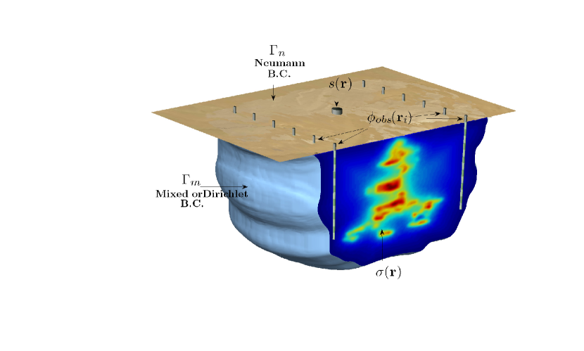
Figure 1: An ERT application: reconstruction of the subsurface conductivity distribution based on the potential measurements at inserted boreholes. A Neumann boundary condition (B.C.) considered for the top surface and a mixed or Dirichlet type B.C. considered for the remaining boundaries

A common geophysical problem associated with the model in (1)–(2) is shown in Fig. 1. In this problem $\Gamma$ consist of $\Gamma_{n}$, the interface between the earth and air where we impose a zero current condition ($\beta=0$) and $\Gamma_{m}$, a surface where the values $\alpha$ and $\beta$ are chosen to model an infinite half-space [26]. As an approximation to an infinite half-space, the boundary condition on $\Gamma_{m}$ may be replaced with a zero potential condition ($\alpha=0$) when $\Gamma_{m}$ is far from the sources of current [27]. Reconstruction of $\sigma$ based on the measurements of $\phi$ at some points in the domain is the goal of this tomography problem.

For simplicity here, we consider only real-valued conductivity (that is the ERT problems) although the approach can easily be adapted for use in estimation of complex valued conductivity as is encountered in EIT as well as conductivity/chargability as are desired in IP experiments. To keep the notation simple, we also consider the case where data are collected from a single source of current. More generally, in a tomographic imaging problem one would illuminate with many sources $s_{p}$ for $p=1,2,\cdots,P.$

Central to the derivation that follows is the impact of a small change in conductivity to the system (1)–(2). Consider a perturbation to the conductivity, $\sigma\rightarrow\sigma+\delta\sigma$ resulting in $\phi\rightarrow\phi+\delta\phi$. Using these in (1)–(2) gives

$$\nabla\cdot\big{(}(\sigma+\delta\sigma)\nabla(\phi+\delta\phi)\big{)} =s \mbox{on}\;\Omega,$$ (3)

$$\alpha(\sigma+\delta\sigma)\frac{\partial}{\partial\mathbf{n}}(\phi+\delta\phi)+\beta(\phi+\delta\phi) =0 \mbox{on}\;\Gamma.$$ (4)

Now, expanding (3) as

$$\nabla\cdot(\sigma\nabla\phi)+\nabla\cdot(\delta\sigma\nabla\phi)+\nabla\cdot(\sigma\nabla\delta\phi)+\nabla\cdot(\delta\sigma\nabla\delta\phi)=s,$$

keeping terms of first order and using (1) in (3) and (2) in (4) yields

$$\nabla\cdot(\delta\sigma\nabla\phi)+\nabla\cdot(\sigma\nabla\delta\phi) =0, \mbox{on}\;\Omega,$$ (5)

$$\alpha(\sigma\frac{\partial}{\partial\mathbf{n}}\delta\phi+\delta\sigma\frac{\partial\phi}{\partial\mathbf{n}})+\beta\delta\phi =0 \mbox{on}\;\Gamma.$$ (6)

The goal of the inverse problem is to estimate $\sigma$ from observations of the potential collected at a finite set of points in space $\mathbf{r}_{i}$, $i=1,2,\cdots,N$. The estimate is obtained by minimizing the least squares cost function

$$J(\sigma) =\frac{1}{2}\sum_{i=1}^{N}\big{(}\phi(\mathbf{r}_{i})-\phi_{obs}(\mathbf{r}_{i})\big{)}^{2}$$

$$=\frac{1}{2}\;\mathbf{E}(\sigma)^{T}\mathbf{E}(\sigma),$$ (7)

where $\phi_{obs}(\mathbf{r}_{i})$ are the observations of potential at location $\mathbf{r}_{i}$ and $\phi(\mathbf{r}_{i})$ is implicitly a function of $\sigma$ through (1)–(2). The length $N$ column vector $\mathbf{E}(\sigma)$ contains the $N$ residuals, $e_{i}(\sigma)=\phi(\mathbf{r}_{i})-\phi_{obs}(\mathbf{r}_{i})$ for $i=1,2,\cdots,N$. A few remarks are in order regarding (7):

• The use of a least squares formulation is not terribly restrictive. For example, a one-norm type of cost function could be accommodated by populating $\mathbf{E}$ with a suitably smoothed version of $|\phi(\mathbf{r}_{i})-\phi_{obs}(\mathbf{r}_{i})|^{1/2}$. Though somewhat tedious, the results in this letter could then be generalized.

• Generalization of (7) to account for weighting of the residuals is also not difficult. To avoid the resulting notational burdens, we choose to not include these details.

• In many cases, the cost function includes both a data misfit term as in (7) as well as additional regularization. We refer the reader to [28] for details concerning the treatment of Tikhonov-type regularization schemes. The adjoint field calculations of interest here pertain only to the data term.

As discussed in Section 1, two type of sensitivities are of interest depending on the nature of the inversion algorithm. Methods based on gradient information such as the steepest decent, require the functional derivative of the cost function with respect to $\sigma$. More formally, a linear integral operator is sought which maps small perturbations of the conductivity, $\delta\sigma$, to corresponding changes in $J$. In the case of Newton type methods and more specifically the Gauss-Newton approach, one requires $N$ linear operators relating $\delta\sigma$ to perturbations in the individual residuals, $\delta e_{i}$. We start with the latter. Subsequently we indicate the changes to the derivation required to obtain the former and also how the adjoint calculations used in the Newton type approaches can be assembled to obtain the gradient-based sensitivity information.

3 Adjoint Field Calculations

To start, we consider the variation in $e_{i}$ due to a small change in $\sigma$. We have

$$\delta e_{i}(\sigma)=\delta\phi(\mathbf{r})|_{\mathbf{r}=\mathbf{r}_{i}},$$

which can be written as a volume integral

$$\delta e_{i}(\sigma)=\int_{\Omega}\delta(\mathbf{r}-\mathbf{r}_{i})\delta\phi(\mathbf{r})\hskip 1.99168ptd\mathbf{r},$$ (8)

where $\delta(.)$ denotes the Dirac delta function. The objective here is to find the linear integral operator relating $\delta e_{i}$ to $\delta\sigma$. Toward this end we define the $i$-th adjoint source $\tilde{s}_{i}$ as

$$\tilde{s}_{i}(\mathbf{r})=\delta(\mathbf{r}-\mathbf{r}_{i}).$$

It is now useful to define the potential, $\tilde{\phi}_{i}$, as the solution to the adjoint system

$$\nabla\cdot(\sigma\nabla\tilde{\phi}_{i}) =\tilde{s}_{i} \mbox{on}\;\Omega,$$ (9)

$$\alpha\sigma\dfrac{\partial\tilde{\phi}_{i}}{\partial\mathbf{n}}+\beta\tilde{\phi}_{i} =0 \text{ on }\Gamma.$$ (10)

Physically, $\tilde{\phi}_{i}$ is the potential field arising from the solution to the adjoint Poisson’s equation (which in this case is the same as the original since Poisson’s equation is self-adjoint) due to a point source of amplitude unity located at the $i$-th receiver. From (8) and (9) we conclude that the perturbation to the residuals can be written in terms of the adjoint field as

$$\delta e_{i}(\sigma)=\int_{\Omega}\nabla\cdot(\sigma\nabla\tilde{\phi}_{i})\delta\phi(\mathbf{r})\hskip 1.99168ptd\mathbf{r}.$$ (11)

The goal is to find a collection of kernel functions, $k_{i}(\mathbf{r})$ such that (11) can be expressed as

$$\delta e_{i}(\sigma)=\int_{\Omega}k_{i}(\mathbf{r})\delta\sigma(\mathbf{r})\hskip 1.99168ptd\mathbf{r}.$$ (12)

The resulting kernels are known as the Frechét derivative of $e_{i}$ with respect to $\sigma$ [29].

To find these kernels, we make extensive use of the following identity derived from Green’s theorem [30] for vector function $\mathbf{F}$ and scalar function $g$

$$\int_{\Omega}\mathbf{F}\cdot\nabla g\hskip 1.99168ptd\mathbf{r}+\int_{\Omega}g(\nabla\cdot\mathbf{F})\hskip 1.99168ptd\mathbf{r}=\int_{\Gamma}g\mathbf{F}\cdot d\mathcal{S},$$ (13)

where $\int\mathbf{V}\cdot d\mathcal{S}=\int(\mathbf{V}\cdot\mathbf{n})\;dS$ denotes the surface integral over $\Gamma$ of the normal component of the vector field $\mathbf{V}$.

We begin by taking $g=\delta\phi$ and $\mathbf{F}=\sigma\nabla\tilde{\phi}_{i}$ in (11) to obtain

$$\delta e_{i}(\sigma)=-\int_{\Omega}\sigma(\nabla\tilde{\phi}_{i})\cdot(\nabla\delta\phi)\hskip 1.99168ptd\mathbf{r}+\int_{\Gamma}\sigma\nabla\tilde{\phi}_{i}\delta\phi\cdot d\mathcal{S}.$$ (14)

Next using $g=\tilde{\phi}_{i}$ and $\mathbf{F}=\sigma\nabla\delta\phi$ in the first term on the right hand side of (14), we have

$$\delta e_{i}(\sigma) =\int_{\Omega}\tilde{\phi}_{i}\nabla\cdot(\sigma\nabla\delta\phi)\hskip 1.99168ptd\mathbf{r}$$

$$-\int_{\Gamma}\sigma(\nabla\delta\phi)\tilde{\phi}_{i}\cdot d\mathcal{S}+\int_{\Gamma}\sigma\nabla\tilde{\phi}_{i}\delta\phi\cdot d\mathcal{S}.$$ (15)

From (5), $\nabla\cdot\delta\sigma\nabla\phi=-\nabla\cdot\sigma\nabla\delta\phi$ which we use in the first term on the right hand side of (15) to arrive at

$$\delta e_{i}(\sigma)= -\int_{\Omega}\tilde{\phi}_{i}\nabla\cdot(\delta\sigma\nabla\phi)\hskip 1.99168ptd\mathbf{r}$$

$$-\int_{\Gamma}\sigma(\nabla\delta\phi)\tilde{\phi}_{i}\cdot d\mathcal{S}+\int_{\Gamma}\sigma(\nabla\tilde{\phi}_{i})\delta\phi\cdot d\mathcal{S}.$$ (16)

Appealing once more to (13) with $g=\tilde{\phi}_{i}$ and $\mathbf{F}=\delta\sigma\nabla\phi$ in the first term of (16) gives

$$\delta e_{i}(\sigma) =\int_{\Omega}\delta\sigma(\nabla\tilde{\phi}_{i})\cdot(\nabla\phi)\hskip 1.99168ptd\mathbf{r}$$ (17)

$$-\int_{\Gamma}\Big{(}\sigma(\nabla\delta\phi)\tilde{\phi}_{i}+\delta\sigma(\nabla\phi)\tilde{\phi}_{i}-\sigma(\nabla\tilde{\phi}_{i})\delta\phi\Big{)}\cdot d\mathcal{S}.$$

We now rewrite the surface integral term on the right hand side of (17) as the integration over the normal component

$$\mathscr{I}=\int_{\Gamma}\Big{(}\sigma\frac{\partial}{\partial\mathbf{n}}\delta\phi\tilde{\phi}_{i}+\delta\sigma\frac{\partial\phi}{\partial\mathbf{n}}\tilde{\phi}_{i}-\sigma\dfrac{\partial\tilde{\phi}_{i}}{\partial\mathbf{n}}\delta\phi\Big{)}dS,$$ (18)

and show that it is zero. For this purpose we multiply both sides of (10) by $\delta\phi$ to arrive at

$$\beta\delta\phi\tilde{\phi}_{i}+\alpha\sigma\dfrac{\partial\tilde{\phi}_{i}}{\partial\mathbf{n}}\delta\phi=0.$$ (19)

Using (6) to replace the term $\beta\delta\phi$ in (19) results in

$$-\alpha\Big{(}\sigma\frac{\partial}{\partial\mathbf{n}}\delta\phi\tilde{\phi}_{i}+\delta\sigma\frac{\partial\phi}{\partial\mathbf{n}}\tilde{\phi}_{i}-\sigma\dfrac{\partial\tilde{\phi}_{i}}{\partial\mathbf{n}}\delta\phi\Big{)}=0,\qquad\text{on}\;\Gamma.$$ (20)

The expression within the brackets in (20) is the same as the integrand in (18). Considering this term, if $\alpha\neq 0$ for $\Gamma_{\alpha}\subset\Gamma$, then clearly the inside bracket expression becomes zero on $\Gamma_{\alpha}$. For the remaining surface $\Gamma\setminus\Gamma_{\alpha}$ that $\alpha=0$, we certainly have $\beta\neq 0$ since $\alpha$ and $\beta$ may not be simultaneously zero and using this fact in (6) and (10) would result in $\delta\phi=0$ and $\tilde{\phi}_{i}=0$ which again make the inside bracket term zero. Therefore for all $\mathbf{r}\in\Gamma$ the inside bracket term is zero and hence the surface integral in (18) vanishes, resulting in

$$\delta e_{i}(\sigma)=\int_{\Omega}\delta\sigma(\nabla\tilde{\phi}_{i})\cdot(\nabla\phi)\hskip 1.99168ptd\mathbf{r}.$$ (21)

This result expresses the perturbation to $e_{i}$ as a linear operator acting on $\delta\sigma$ as desired, and accordingly identifying the kernel function in (16) as $k_{i}(\mathbf{r})=\big{(}\nabla\tilde{\phi}_{i}(\mathbf{r})\big{)}\cdot\big{(}\nabla\phi(\mathbf{r})\big{)}$.

In case of a system with nonhomogeneous boundary condition

$$\nabla\cdot(\sigma\nabla\phi) =s \mbox{in}\;\Omega,$$ (22)

$$\alpha\sigma\frac{\partial\phi}{\partial\mathbf{n}}+\beta\phi =\xi \mbox{on}\;\Gamma,$$ (23)

perturbing $\sigma\rightarrow\sigma+\delta\sigma$ and $\phi\rightarrow\phi+\delta\phi$ would result in the same equations as (5)–(6) and $\xi$ will be cancelled. Based on this result, by solving the same forward problem as (9)–(10) and finding $\tilde{\phi}_{i}$, identical forms of sensitivity as (21) will be obtained for the case of nonhomogeneous boundary condition. However, we should note that although the sensitivity results are valid, by definition of an adjoint system, (9)–(10) is not the adjoint of the nonhomogeneous system (22)–(23). More details in this regard are provided in the Appendix.

In cases where gradient decent-type optimization methods are used for imaging, one requires the functional derivative of the cost function, $J(\sigma)$ in (7) with respect to the conductivity. The required variation now is

$$\delta J(\sigma)=\sum_{i=1}^{N}\big{(}\phi(\mathbf{r}_{i})-\phi_{obs}(\mathbf{r}_{i})\big{)}\delta\phi(\mathbf{r}_{i}),$$

which similarly may be rewritten in an integral form as

$$\delta J(\sigma) =\sum_{i=1}^{N}\big{(}\phi(\mathbf{r}_{i})-\phi_{obs}(\mathbf{r}_{i})\big{)}\int_{\Omega}\delta(\mathbf{r}-\mathbf{r}_{i})\delta\phi(\mathbf{r})\hskip 1.99168ptd\mathbf{r}$$

$$=\int_{\Omega}\!\!\Big{(}\!\sum_{i=1}^{N}\!\big{(}\phi(\mathbf{r}_{i})-\phi_{obs}(\mathbf{r}_{i})\big{)}\delta(\mathbf{r}-\mathbf{r}_{i})\!\Big{)}\delta\phi(\mathbf{r})\hskip 1.99168ptd\mathbf{r}.$$

There are two ways to determine the resulting Frechét derivative. On the one hand, if we define the composite adjoint source

$$\tilde{s}(\mathbf{r})=\sum_{i=1}^{N}\big{(}\phi(\mathbf{r}_{i})-\phi_{obs}(\mathbf{r}_{i})\big{)}\delta(\mathbf{r}-\mathbf{r}_{i})$$ (24)

the derivation provided above follows unaltered and we conclude

$$\delta J(\sigma)=\int_{\Omega}\delta\sigma(\nabla\tilde{\phi})\cdot(\nabla\phi)\hskip 1.99168ptd\mathbf{r},$$ (25)

where now $\tilde{\phi}$ is a single adjoint field computed according to (9)–(10) with $\tilde{s}$ replacing $\tilde{s}_{i}$. Thus, for gradient decent methods, one requires only two solutions of Poisson’s equation: one for the source and one for the composite adjoint source as opposed to $1+N$ solves needed for a Gauss-Newton scheme. Alternatively, since $\tilde{s}=\sum_{i}\big{(}\phi(\mathbf{r}_{i})-\phi_{obs}(\mathbf{r}_{i})\big{)}\tilde{s}_{i}$, by the linearity of Poisson’s equation and (24)

$$\delta J(\sigma) =\sum_{i=1}^{N}\big{(}\phi(\mathbf{r}_{i})-\phi_{obs}(\mathbf{r}_{i})\big{)}\delta e_{i}(\sigma)$$

$$=\sum_{i=1}^{N}\big{(}\phi(\mathbf{r}_{i})-\phi_{obs}(\mathbf{r}_{i})\big{)}\int_{\Omega}\delta\sigma(\nabla\tilde{\phi}_{i})\cdot(\nabla\phi)\hskip 1.99168ptd\mathbf{r},$$

which is the desired link between the two uses for the adjoint field in sensitivity calculations.

As a concrete example, consider a 3D imaging problem where $\sigma(\mathbf{r})$ is discretized to form a vector $\boldsymbol{\sigma}=[\sigma_{1},\cdots,\sigma_{M}]^{T}$. Here the $j$-th element corresponds to a voxel $\Omega_{j}$ in the domain, over which the conductivity is assumed to be uniformly $\sigma_{j}$. To iteratively minimize the least squares problem (7) using a gradient descent approach, the $k$-th iteration to find $\boldsymbol{\sigma}^{(k+1)}$ is performed by moving along the negative direction of $\nabla J$ as

$$\boldsymbol{\sigma}^{(k+1)}-\boldsymbol{\sigma}^{(k)} =-\gamma^{(k)}\nabla J^{(k)}$$

$$=-\gamma^{(k)}(\nabla\mathbf{E}^{(k)})^{T}\mathbf{E}^{(k)}$$

where $\gamma^{(k)}>0$ is a step size [31]. On the other hand, for Newton type methods, the updating is performed through solving the following system for $\boldsymbol{\sigma}^{(k+1)}$

$$\mathbf{B}^{(k)}(\boldsymbol{\sigma}^{(k+1)}-\boldsymbol{\sigma}^{(k)})=-(\nabla\mathbf{E}^{(k)})^{T}\mathbf{E}^{(k)},$$

where $\mathbf{B}$ is a positive definite approximation to the Hessian of $J$, such as $(\nabla\mathbf{E})^{T}\nabla\mathbf{E}$ in a Guass-Newton approach or $(\nabla\mathbf{E})^{T}\nabla\mathbf{E}+\gamma\mathbf{I}$ in a Levenberg-Marquardt case [31]. Clearly, in using a gradient descent approach only $\nabla J$ (basically the product of $\nabla\mathbf{E}^{T}\mathbf{E}$) is required at every iteration while in a Gauss-Newton approach $\nabla\mathbf{E}$ itself is required. The $(i,j)$-th element of the $N\times M$ matrix $\nabla\mathbf{E}$ is $\partial e_{i}/\partial\sigma_{j}$. By taking $\delta\sigma$ in (21) to be $\delta\sigma_{j}\chi_{\Omega_{j}}(\mathbf{r})$ with $\chi_{A}$ the indicator function over a set $A$, we have

$$\frac{\partial e_{i}}{\partial\sigma_{j}}=\int_{\Omega_{j}}(\nabla\tilde{\phi}_{i})\cdot(\nabla\phi)\hskip 1.99168ptd\mathbf{r}.$$

Thus, the cost to calculate $\nabla\mathbf{E}$ is solving one forward problem to compute $\phi$, $N$ adjoint problems to determine $\tilde{\phi}_{i}$, and, for each $i$ the evaluation of $M$ integrals to determine each row of the matrix. However, in a gradient descent approach where only the vector $\nabla J$ of length $N$ is required each element may be calculated through (25) as

$$\frac{\partial J}{\partial\sigma_{j}}=\int_{\Omega_{j}}(\nabla\tilde{\phi})\cdot(\nabla\phi)\hskip 1.99168ptd\mathbf{r},$$

which requires solving one forward problem to compute $\phi$, one adjoint problem to obtain $\tilde{\phi}$ and $N$ integrations.

4 Conclusion

We presented explicit and generalizable methods of calculating the sensitivity in inversion of Poisson’s type problems. For problems that minimize the misfit between the data and the model for the purpose of inversion, gradient descent methods or Newton type methods such as the Gauss-Newton and the Levenberg-Marquardt may be used. From an implementation point of view, gradient descent methods are easy to implement, but iteratively slow and have variable scaling issues [31]. On the other hand Newton type methods have a faster convergence rate and are robust to variable scalings but can be computationally expensive. Based on the nature of the problem and the available computing resources either methods may be desirable in solving an inverse problem. It is highlighted that to maintain efficiency, two different adjoint problems need to be solved to obtain the sensitivity information in each inversion scheme. This paper beside providing a step by step derivation of the sensitivities for the Poisson’s equation with general type of boundary condition, clarifies the distinction and the relationship between the two forms of inversion for various types of applications.

5 Appendix

By definition, for the systems (22)–(23) and (9)–(10) to be adjoints we must have

$$\int_{\Omega}\nabla\cdot(\sigma\nabla\tilde{\phi}_{i})\phi\hskip 1.99168ptd\mathbf{r}=\int_{\Omega}\nabla\cdot(\sigma\nabla\phi)\tilde{\phi}_{i}\hskip 1.99168ptd\mathbf{r}.$$ (26)

Applying the identity (13) twice to $\int_{\Omega}\nabla\cdot(\sigma\nabla\tilde{\phi}_{i})\phi\hskip 1.99168ptd\mathbf{r}$, first with $g=\phi$ and $F=\sigma\nabla\tilde{\phi}_{i}$, and next with $g=\tilde{\phi}_{i}$ and $F=\sigma\nabla\phi$ results in

$$\int_{\Omega}\nabla\cdot(\sigma\nabla\tilde{\phi}_{i})\phi\hskip 1.99168ptd\mathbf{r}- \int_{\Omega}\nabla\cdot(\sigma\nabla\phi)\tilde{\phi}_{i}\hskip 1.99168ptd\mathbf{r}$$

$$= \int_{\Gamma}\Big{(}\sigma\nabla\tilde{\phi}_{i}\phi-\sigma\nabla\phi\tilde{\phi}_{i}\Big{)}\cdot d\mathcal{S}$$ (27)

We next split the surface integral on the right hand side of (27) over regions $\Gamma_{\alpha}$ where $\alpha\neq 0$ and $\Gamma\setminus\Gamma_{\alpha}$ where $\alpha=0$. On $\Gamma_{\alpha}$ using (10) and (23) we have

$$\sigma\frac{\partial\tilde{\phi}_{i}}{\partial\mathbf{n}}\phi-\sigma\frac{\partial\phi}{\partial\mathbf{n}}\tilde{\phi}_{i}=-\frac{\xi\tilde{\phi}_{i}}{\alpha},$$ (28)

and over $\Gamma\setminus\Gamma_{\alpha}$ that $\alpha=0$ and $\beta\neq 0$, using (10) and (23) yields $\tilde{\phi}_{i}=0$ and $\phi=\xi/\beta$ and therefore

$$\sigma\frac{\partial\tilde{\phi}_{i}}{\partial\mathbf{n}}\phi-\sigma\frac{\partial\phi}{\partial\mathbf{n}}\tilde{\phi}_{i}=\frac{\sigma\xi}{\beta}\frac{\partial\tilde{\phi}_{i}}{\partial\mathbf{n}}.$$ (29)

Based on (28) and (29) we rewrite (27) as

$$\int_{\Omega}\nabla\cdot(\sigma\nabla\tilde{\phi}_{i})\phi\hskip 1.99168ptd\mathbf{r}- \int_{\Omega}\nabla\cdot(\sigma\nabla\phi)\tilde{\phi}_{i}\hskip 1.99168ptd\mathbf{r}$$ (30)

$$= -\int_{\Gamma\setminus\Gamma_{\alpha}}\frac{\xi\tilde{\phi}_{i}}{\alpha}dS+\int_{\Gamma_{\alpha}}\frac{\sigma\xi}{\beta}\frac{\partial\tilde{\phi}_{i}}{\partial\mathbf{n}}dS.$$

Comparing (30) to (26) shows that for the systems (22)–(23) and (9)–(10) to be adjoints the expression on the right hand side of (30) needs to be zero and this is not generally the case. Clearly (26) holds for the homogeneous case ($\xi=0$) and the two systems are adjoints as mentioned in the text.

References

- [1] A. Ramirez, W. Daily, D. LaBrecque, E. Owen, and D. Chesnut, “Monitoring an underground steam injection process using electrical resistance tomography,” Water Resources Research, vol. 29, no. 1, pp. 73–87, 1993.
- [2] M. Cheney, D. Isaacson, and J. Newell, “Electrical impedance tomography,” SIAM review, vol. 41, no. 1, pp. 85–101, 1999.
- [3] D. Oldenburg and Y. Li, “Inversion of induced polarization data,” Geophysics, vol. 59, no. 9, pp. 1327–1341, 1994.
- [4] M. Soleimani and W. Lionheart, “Nonlinear image reconstruction for electrical capacitance tomography using experimental data,” Measurement Science and Technology, vol. 16, p. 1987, 2005.
- [5] C. Xie, S. Huang, B. Hoyle, R. Thorn, C. Lenn, D. Snowden, and M. Beck, “Electrical capacitance tomography for flow imaging: system model for development of image reconstruction algorithms and design of primary sensors,” vol. 139, no. 1, pp. 89–98, 1992.
- [6] S. Arridge, “Optical tomography in medical imaging,” Inverse problems, vol. 15, p. R41, 1999.
- [7] E. Somersalo, M. Cheney, and D. Isaacson, “Existence and uniqueness for electrode models for electric current computed tomography,” SIAM Journal on Applied Mathematics, vol. 52, no. 4, pp. 1023–1040, 1992.
- [8] O. Dorn, H. Bertete-Aguirre, J. Berryman, and G. Papanicolaou, “A nonlinear inversion method for 3d electromagnetic imaging using adjoint fields,” Inverse Problems, vol. 15, p. 1523, 1999.
- [9] O. Dorn, E. Miller, and C. Rappaport, “A shape reconstruction method for electromagnetic tomography using adjoint fields and level sets,” Inverse problems, vol. 16, p. 1119, 2000.
- [10] A. Abubakar and P. van den Berg, “Nonlinear inversion in electrode logging in a highly deviated formation with invasion using an oblique coordinate system,” Geoscience and Remote Sensing, IEEE Transactions on, vol. 38, no. 1, pp. 25–38, 2000.
- [11] A. Abubakar and P. Berg, “The contrast source inversion method for location and shape reconstructions,” Inverse Problems, vol. 18, p. 495, 2002.
- [12] A. Abubakar, P. van den Berg, and S. Semenov, “A robust iterative method for born inversion,” Geoscience and Remote Sensing, IEEE Transactions on, vol. 42, no. 2, pp. 342–354, 2004.
- [13] X. Tai and T. Chan, “A survey on multiple level set methods with applications for identifying piecewise constant functions,” Int. J. Numer. Anal. Model, vol. 1, no. 1, pp. 25–47, 2004.
- [14] M. Ben Hadj Miled and E. Miller, “A projection-based level-set approach to enhance conductivity anomaly reconstruction in electrical resistance tomography,” Inverse Problems, vol. 23, p. 2375, 2007.
- [15] O. Dorn and D. Lesselier, “Level set methods for inverse scattering,” Inverse Problems, vol. 22, p. R67, 2006.
- [16] W. Lionheart, “Eit reconstruction algorithms: pitfalls, challenges and recent developments,” Physiological Measurement, vol. 25, p. 125, 2004.
- [17] N. Polydorides and W. Lionheart, “A matlab toolkit for three-dimensional electrical impedance tomography: a contribution to the electrical impedance and diffuse optical reconstruction software project,” Measurement science and technology, vol. 13, p. 1871, 2002.
- [18] A. Aghasi, M. Kilmer, and E. L. Miller, “Parametric level set methods for inverse problems,” SIAM Journal on Imaging Sciences, vol. 4, no. 2, pp. 618–650, 2011. [Online]. Available: http://link.aip.org/link/?SII/4/618/1
- [19] E. Chung, T. Chan, and X. Tai, “Electrical impedance tomography using level set representation and total variational regularization,” Journal of Computational Physics, vol. 205, no. 1, pp. 357–372, 2005.
- [20] T. Rylander, P. Hashemzadeh, and M. Viberg, “Reconstruction of metal protrusion on flat ground plane,” Microwaves, Antennas & Propagation, IET, vol. 4, no. 11, pp. 1746–1755, 2010.
-
[21]
S. Nordebo, R. Bayford, B. Bengtsson, A. Fhager, M. Gustafsson,
P. Hashemzadeh,
B. Nilsson, T. Rylander, and T. Sj
”oden, “An adjoint field approach to fisher information-based sensitivity analysis in electrical impedance tomography,” Inverse Problems, vol. 26, p. 125008, 2010. - [22] D. Geselowitz, “An application of electrocardiographic lead theory to impedance plethysmography,” Biomedical Engineering, IEEE Transactions on, no. 1, pp. 38–41, 1971.
- [23] T. Günther, C. Rücker, and K. Spitzer, “Three-dimensional modelling and inversion of dc resistivity data incorporating topography–ii. inversion,” Geophysical Journal International, vol. 166, no. 2, pp. 506–517, 2006.
- [24] A. Abubakar, T. Habashy, V. Druskin, L. Knizhnerman, and D. Alumbaugh, “2.5 d forward and inverse modeling for interpreting low-frequency electromagnetic measurements,” Geophysics, vol. 73, p. F165, 2008.
- [25] S. Norton, “Iterative inverse scattering algorithms: Methods of computing frechet derivatives,” The Journal of the Acoustical Society of America, vol. 106, p. 2653, 1999.
- [26] D. Pollock and O. Cirpka, “Temporal moments in geoelectrical monitoring of salt tracer experiments,” Water Resources Research, vol. 44, no. 12, p. W12416, 2008.
- [27] A. Tripp, G. Hohmann, C. Swift et al., “Two-dimensional resistivity inversion,” Geophysics, vol. 49, no. 10, pp. 1708–1717, 1984.
- [28] A. Tikhonov and V. Arsenin, Solutions of ill-posed problems. Winston Washington, DC:, 1977.
- [29] J. Dieudonné and S. O. service), Foundations of modern analysis. Academic Press Orlando, FL, 1969.
- [30] J. Marsden and A. Tromba, Vector calculus. WH Freeman, 2003.
- [31] D. Bertsekas, Nonlinear programming. Athena Scientific Belmont, MA, 1999.