Comparative study of quantum dynamics of a few bosons in a one-dimensional split hard-wall trap: exact results versus Bose-Hubbard-model approximations

Abstract

We study the dynamical properties of a few bosons confined in an one-dimensional split hard wall trap with the interaction strength varying from the weakly to strongly repulsive regime. The system is initially prepared in one side of the double well by setting the barrier strength of the split trap to be infinity and then the barrier strength is suddenly changed to a finite value. Both exact diagonalization method and Bose-Hubbard model (BHM) approximation are used to study the dynamical evolution of the initial system. The exact results based on exact diagonaliztion verify the enhancement of correlated tunneling in the strongly interacting regime. Comparing results obtained by two different methods, we conclude that one-band BHM approximation can well describe the dynamics in the weakly interacting regime, but is not efficient to give quantitatively consistent results in the strongly interacting regime. Despite of the quantitative discrepancy, we validate that the form of correlated tunneling gives an important contribution to tunneling in the large interaction regime. To get a quantitative description for the dynamics of bosons in the strongly interacting regime, we find that a multi-band BHM approximation is necessary.

I Introduction

Bose-Einstein condensates in double-well potentials have attracted much attention in the past decades. As a paradigm model for studying the competition effect of quantum tunneling and interaction, the double well systems have been widely studied from many aspects PRA77063601 ; PRA593868 ; JPA381235 ; PRA78013604 ; Smerzi ; PRA554318 ; RMP73307 ; Liujie ; Raghavan ; Mahmud . Due to the experimental progress in manipulating ultracold atomic gases, both the trap potential and interaction between atoms can be implemented with unprecedented tunability RMP , and thus the dynamics of many-body quantum states of interacting bosons can be experimentally explored by loading the ultracold atoms in double wells. For the atomic double-well system, the atom-atom interactions in Bose-Einstein condensates have been found to play important roles in the dynamics of the system. The competition between tunneling and interaction leads to many rich and interesting effects, such as the Josephson oscillation and self-trapping phenomena Smerzi ; PRA554318 ; RMP73307 ; Liujie ; PRA593868 ; Raghavan ; Mahmud . Moreover, novel correlated tunneling dynamics in interacting atomic systems characterized by a small number of particles has recently been observed experimentally Folling , which attracted particular attention in the study of the dynamics of few-atom systems Zollner ; Liang .

So far most of theoretical works for double-well systems are based on the two-mode approximation Smerzi ; PRA554318 ; RMP73307 ; Liujie ; Raghavan ; PRA593868 . For atoms confined in a double well potential, if all of them are prepared in one well initially, they will oscillate in the form of Josephson oscillation for weak enough interaction, or they will stay in one well (self-trapping) when the interaction is above a critical value. Both the Josephson oscillation and self-trapping phenomena can be understood within the two-mode approximation and have been observed experimentally in cold atomic systems Albiez . However, if interactions are strong enough, the mean-field theory and the two-mode approximation are not expected to be valid as higher orbits are occupied. In the strongly interacting regime, strong interactions between atoms may fundamentally alter the tunnel dynamics and result in a correlated tunneling, which was explored most recently in ultracold atoms Zollner ; Liang . Theoretically, the correlated paring tunneling was studied by multi-configuration time-dependent Hartree method Zollner ; Sakmann and also in the scheme of the extended Bose-Hubbard model with an additional term of correlated pair tunneling Liang . In order to understand the dynamics of double well systems from weakly to strongly interacting regime in an unified scheme, in this work we study the dynamical properties of a few bosons confined in a one-dimensional (1D) split hard wall trap with the repulsive interaction strength varying from zero to infinity. Experimentally, the effective interaction strength can be tuned by using Feshbach resonance or the confinement-induced resonance to the strongly interacting Tonks-Girardeau (TG) limit Paredes ; Weiss , which makes it possible to explore the novel dynamics even in the TG limit.

In the TG limit, the bosonic systems exhibit the feature of fermionization Girardeau ; Cederbaum ; Hao1 ; Hao2 ; Zollner2 ; Deuretzbacher . In the strongly interacting regime, the mean field theory generally fails to describe the properties of fermionization. In order to characterize the crossover from weakly interacting condensation to strongly interacting TG gas, some sophistical theoretical methods, such as the exact diagonalization method Deuretzbacher ; Hao2 ; PRA78013604 and multi-orbital self-consistent Hartree method Zollner2 ; Cederbaum have been applied to study the static few-boson systems. In this work, we shall apply the exact diagonalization method to study the dynamical problem in the 1D double-well system. The exact diagonalization method can produce numerically exact results and allows us to give an unified description for both the weakly and strongly interacting regime. As a comparison, we also investigate the dynamics based on the two-site Bose-Hubbard model by considering both the two-mode and muti-mode approximations. Comparing the results obtained from different methods, we conclude that one-band (two-mode) BHM approximation is efficient to describe dynamics in small interaction regime, but the multi-band BHM approximation is needed if we want to describe the dynamics of bosons with large interaction quantitatively. We also validate that the form of pair tunneling gives an important contribution to tunneling in the large interaction regime.

II Model and method

We consider a few bosons with mass $m$ confined in an one-dimensional split hard wall trap, which is described by the Hamiltonian ($\hbar=m=1$)

$$\widehat{H} = \int\widehat{\psi}^{\dagger}(x)\left[-\frac{1}{2}\frac{\partial^{2}}{\partial x^{2}}+V(x)+\kappa\delta(x)\right]\widehat{\psi}(x)dx+$$ (1)

$$c\int\widehat{\psi}^{\dagger}(x)\widehat{\psi}^{\dagger}(x^{\prime})\delta(x-x^{\prime})\widehat{\psi}(x)\widehat{\psi}(x^{\prime})dxdx^{\prime}.$$

Here $V(x)$ is a hard wall trap which is zero in the region $(-a,a)$ and infinite outside, $\kappa$ is a tunable parameter which describes the strength of zero-ranged barrier at the center of the trap, and $c$ is the interaction strength between particles determined by the effective 1D s-wave scattering length. Here the double well is modeled by the 1D split hard-wall trap with a $\delta$-type barrier located at the origin and the tunneling amplitude between the left and right wells can be tuned by the barrier strength $\kappa$ PRA77063601 ; PRA78013604 . To study the tunneling dynamics, the barrier strength $\kappa$ is initially set to be infinity and the system is prepared in the ground state of the left well. At time $t=0$, we suddenly change $\kappa$ to a finite value and study the dynamical evolution of the initially prepared system.

For $c=0$, the single particle stationary Schrödinger equation associated with the Hamiltonian (1) can be written as

$$\left[-\frac{1}{2}\frac{\partial^{2}}{\partial x^{2}}+V(x)+\kappa\delta(x)\right]\varphi_{n}(x)=\epsilon_{n}\varphi_{n}(x),$$ (2)

where $\varphi_{n}(x)$ are the complete set of orthonormal eigenfunctions and $\epsilon_{n}$ the corresponding eigenenergies. Here $n=1,2,3,\cdots$ gives the ordering number of the single-particle energies. According to the parity symmetry of the eigenfunctions, the state $\varphi_{n}(x)$ is symmetric for odd $n$ ($n=2i-1$) and antisymmetric for even $n$ ($n=2i$). The single-particle energies are ordered alternatively corresponding to symmetric and antisymmetric states. For convenience, we also represent $\varphi_{2i-1}(x)=\varphi_{i,S}(x)$ and $\varphi_{2i}(x)=\varphi_{i,A}(x)$ with the subscript $S$ ($A$) indicating the symmetric (antisymmetric) function. The single-particle antisymmetric eigenfunctions are $\varphi_{i,A}(x)=\frac{1}{\sqrt{a}}\sin(\frac{i\pi x}{a}),$ $i=1,2,3,...$ with their corresponding eigenenergies $\epsilon_{i,A}=\epsilon_{2i}=(i\pi/a)^{2}/2$, and the single-particle symmetric eigenfunctions are $\varphi_{i,S}(x)=C[\cos(px)-\frac{\kappa}{p}\sin(px)]\theta(-x)+C[\cos(px)+\frac{\kappa}{p}\sin(px)]\theta(x)$ with their corresponding eigenenergies $\epsilon_{i,S}=\epsilon_{2i-1}=p^{2}/2$, where the wave vector $p$ is determined by transcend equation $p/\kappa+\tan(pa)=0$ and $C$ is the normalization constant. It is true that the barrier only influences symmetric eigenfunctions, but does not influence antisymmetric eigenfunctions for any barrier strength $\kappa$. Further, the $(2i-1)$-th eigenenergy is close to the $2i$-th eigenenergy ($i=1,2,3...$) gradually with the increase of barrier strength and they become degenerate in the limit $\kappa\rightarrow\infty$. For simplicity, we set $a=1$ and discuss a large barrier strength $\kappa=50$ in this paper. In this case, single-particle eigenenergies in split hard wall trap are $\epsilon_{1}=4.74341$, $\epsilon_{2}=\pi^{2}/2$, $\epsilon_{3}=18.9764$, $\epsilon_{4}=2\pi^{2}$, $\epsilon_{5}=42,7073,...$ respectively, see Fig.1(a). In contrast to the small energy gap between the $(2i-1)$-th state and the $2i$-th state, there is a relatively very large energy gap between the $2i$-th state and $(2i+1)$-th state, i.e., $\epsilon_{i,A}-\epsilon_{i,S}\ll\epsilon_{i+1,S}-\epsilon_{i,A}$.

Expanding field operators as $\widehat{\Psi}(x)=\sum_{n=1}^{\infty}\varphi_{n}(x)a_{n}$, the many-body Hamiltonian (1) takes the form

$$\widehat{H}=\sum_{n}\epsilon_{n}a_{n}^{{\dagger}}a_{n}+c\sum_{n,m,p,q}I_{nmpq}a_{n}^{{\dagger}}a_{m}^{{\dagger}}a_{p}a_{q},$$ (3)

where $a_{n}^{{\dagger}}(a_{n})$ is bosonic creation (annihilation) operator for a particle in the single particle energy eigenstate $\varphi_{n}$. The interaction integral parameters $I_{nmpq}$ are calculated through $I_{nmpq}=\int_{-a}^{a}\varphi_{n}(x)\varphi_{m}(x)\varphi_{p}(x)\varphi_{q}(x)dx$. The eigenstate of this Hamiltonian can be obtained by numerical exact diagonalization in the subspace of the energetically lowest eigen-states of a noninteracting many-particle system Deuretzbacher ; PRA78013604 .

When the barrier strength $\kappa$ is large, the split hard wall trap can be considered as a double well. Similar to the case of optical lattices, the local Wannier functions $W_{L}^{i}(x)$ $(W_{R}^{i}(x))$ at the left (right) well with the energy band indices $i$ can be defined as $W_{L}^{i}(x)=1/\sqrt{2}(\varphi_{i,S}(x)+\varphi_{i,A}(x))$ and $W_{R}^{i}(x)=1/\sqrt{2}(\varphi_{i,S}(x)-\varphi_{i,A}(x))$. From the symmetry of $\varphi_{i,S}(x)$ and $\varphi_{i,A}(x)$, one observes that $W_{L}^{i}(x)=W_{R}^{i}(-x)$. If we expand the bosonic field operator as, $\widehat{\psi}(x)=\sum_{i}a_{i,L}W_{L}^{i}(x)+\sum_{i}a_{i,R}W_{R}^{i}(x)$ , where $a_{i,L\left(R\right)}$ is the bosonic annihilation operator for a particle at left (right) well, the Hamiltonian can be written as the form of two-site Bose Hubbard model

$$\widehat{H}=\sum_{i,j}(J_{LL}^{ij}a_{i,L}^{\dagger}a_{j,L}+J_{RR}^{ij}a_{i,R}^{\dagger}a_{j,R})+\sum_{i,j}(J_{LR}^{ij}a_{i,L}^{\dagger}a_{j,R}+J_{RL}^{ij}a_{i,R}^{\dagger}a_{j,L})+\sum_{i,j,k,l}\sum_{\alpha,\beta,\gamma,\delta}U^{i,j,k,l}_{\alpha,\beta,\gamma,\delta}a_{i,\alpha}^{\dagger}a_{j,\beta}^{\dagger}a_{k,\gamma}a_{l,\delta}$$ (4)

where the integral $J_{\alpha\beta}^{ij}=\int_{-\infty}^{\infty}dx(W_{\alpha}^{i}(x))^{\ast}H_{0}W_{\beta}^{j}(x)$, with $H_{0}=-\frac{1}{2}\frac{\partial^{2}}{\partial x^{2}}+V(x)+\kappa\delta(x)$ and the interaction integral $U_{\alpha,\beta,\gamma,\delta}^{i,j,k,l}=c\int dx(W_{\alpha}^{i}(x))^{\ast}(W_{\beta}^{j}(x))^{\ast}W_{\gamma}^{k}(x)W_{\delta}^{l}(x)$. The subscripts $\alpha,\beta,\gamma,\delta\in\{L,R\}$ are the well indices and the superscripts $i,j,k,l$$\in\{1,2,3,...\}$ are the energy band indices. Here we note $J^{ij}_{RR}=J^{ij}_{LL}$ for the symmetric double well. The Hamiltonian (4) can be divided into intraband and interband parts, that is

$$\widehat{H}=\sum_{i}\widehat{H}_{i}+\widehat{H}_{interband}.$$ (5)

The $i$-th intraband Hamiltonian can be written as

$$\widehat{H}_{i} = (\epsilon_{i,L}n_{i,L}+\epsilon_{i,R}n_{i,R})+[J_{i}+2(n_{i,L}+n_{i,R}-1)J^{\prime}_{i}](a_{i,L}^{\dagger}a_{i,R}+a_{i,R}^{\dagger}a_{i,L})+$$ (6)

$$U_{0}^{i}[n_{i,L}(n_{i,L}-1)+n_{i,R}(n_{i,R}-1)]+U_{LR}^{i}(a_{i,L}^{\dagger}a_{i,L}^{\dagger}a_{i,R}a_{i,R}+a_{i,R}^{\dagger}a_{i,R}^{\dagger}a_{i,L}a_{i,L}+4n_{i,L}n_{i,R}),$$

where $n_{i,L}=a_{i,L}^{\dagger}a_{i,L}$, $n_{i,R}=a_{i,R}^{\dagger}a_{i,R}$, $\epsilon_{i,L}=J_{LL}^{ii}$, $\epsilon_{i,R}=J_{RR}^{ii}$, $J_{i}=J_{LR}^{ii}=J_{RL}^{ii}$ is the intraband hopping energy between left and right wells, $J^{\prime}_{i}=U_{LLLR}^{iiii}=U_{RRRL}^{iiii}$, $U_{0}^{i}=U_{LLLL}^{iiii}=U_{RRRR}^{iiii}$ is the on site interaction energy and $U_{LR}^{i}\equiv U_{LLRR}^{iiii}$ is the intraband pair hopping energy. It is easy to check that $\epsilon_{i,L}=\epsilon_{i,R}=(\epsilon_{i,S}+\epsilon_{i,A})/2=\mu_{i}$ and $J_{i}=(\epsilon_{i,S}-\epsilon_{i,A})/2$. The interband Hamiltonian reads

$$\widehat{H}_{interband}=\sum_{i\neq j}\sum_{\alpha,\beta,\gamma,\delta}U^{i,j}_{\alpha,\beta,\gamma,\delta}(a_{i,\alpha}^{\dagger}a_{j,\beta}^{\dagger}a_{i,\gamma}a_{j,\delta}+a_{i,\alpha}^{\dagger}a_{j,\beta}^{\dagger}a_{j,\gamma}a_{i,\delta})\\ +\sum_{i,j,k,l}^{\prime}\sum_{\alpha,\beta,\gamma,\delta}U^{i,j,k,l}_{\alpha,\beta,\gamma,\delta}a_{i,\alpha}^{\dagger}a_{j,\beta}^{\dagger}a_{k,\gamma}a_{l,\delta}$$

where $U^{i,j}_{\alpha,\beta,\gamma,\delta}=U^{i,j,i,j}_{\alpha,\beta,\gamma,\delta}=U^{i,j,j,i}_{\alpha,\beta,\gamma,\delta}$ and the summation $\sum^{\prime}$ in the second part contains three-band terms where only three different energy band indices exist and four-band terms with $i\neq j\neq k\neq l$. Most interband interaction terms are very small except for terms of $U_{LLLL}^{ij}$ and $U_{RRRR}^{ij}$ defined on the same site and between the $i$th and $j$th bands. For the split system with barrier strength $\kappa=50$, we have $\epsilon_{i,L}=\epsilon_{i,R}=4.83911$, $J_{1}=-0.0957$, $U_{0}^{1}=1.48446c$, $J^{\prime}_{1}=-0.00366c$, $U_{LR}^{1}=0.0003c$ and $U_{LLLL}^{12}=0.98866c$, while the interaction strengths containing three or four energy band indices are very small, for example $U_{LLLL}^{1233}=-0.000969c$ and $U_{LLRR}^{1234}=-0.00107c$ .

Now we turn to consider the dynamical behavior for the $N$-boson system. Initially (for $t<0$), the barrier strength $\kappa$ is set to infinity and $N$ bosons are prepared in the ground state of the left well. In this case, the split hard-wall trap actually reduces to two separated hard-wall traps, so the eigenvalues and eigenfunctions of a single particle in the left well are $(\pi n/a)^{2}/2$ and $\varphi_{n}(x)=-\sqrt{2/a}\sin(n\pi x/a)$, with $n=1,2,3...$ respectively. Then at $t=0$, $\kappa$ is suddenly changed to a finite value, for example $\kappa=50$ in the present work, and the corresponding Hamiltonian is $\widehat{H}_{f}=\widehat{H}(\kappa=50)$. After $\kappa$ is changed, the time-dependant wave function is given by

$$|\Psi(t)\rangle=e^{-i\widehat{H}_{f}t}|\Psi(0)\rangle=\sum_{n=1}^{\infty}C_{n}e^{-iE_{n}t}|\Phi_{n}\rangle,$$ (7)

in which weight coefficients are $C_{n}=\langle\Phi_{n}|\Psi(0)\rangle$ and they satisfy normalization condition $\sum_{n=1}^{\infty}C_{n}^{2}=1$. Here $\Phi_{n}$ and $E_{n}$ are the eigenstates and eigenvalues of $\widehat{H}_{f}$, respectively. In order to see how the initial state trapped in the left trap evolves, we shall use revival probability

$$F(t) = |\langle\Psi(t)|\Psi(0)\rangle|^{2}$$ (8)

$$= 1-4\sum_{n<m}C_{n}^{2}C_{m}^{2}\sin^{2}[(E_{n}-E_{m})t/2],$$

the reduced single-particle density matrix

$$\rho(x,x^{\prime},t)=\langle\Psi(t)|\widehat{\Psi}^{\dagger}(x)\widehat{\Psi}(x^{\prime})|\Psi(t)\rangle,$$ (9)

and pair correlation function

$$g^{(2)}(x_{1},x_{2},t)=\langle\Psi(t)|\widehat{\Psi}^{\dagger}(x_{1})\widehat{\Psi}^{\dagger}(x_{2})\widehat{\Psi}(x_{1})\widehat{\Psi}(x_{2})|\Psi(t)\rangle$$ (10)

after time $t$ to describe the dynamics in split hard-wall trap system.

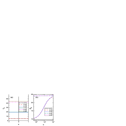
Figure 1: (a)Single-particle energy levels for the split hard wall trap with $\kappa=50$. (b) The eigenenergy of two interacting bosons changing with the interaction strength $c$ in the split hard wall trap with $\kappa=50$.

III results and discussions

Before studying the quantum dynamics of many-body systems, we first recall the tunneling dynamics of a single atom. If there is only one boson in this split hard wall trap, the initial state is just the ground state of left well, that is $\Psi(0)=-\sqrt{2}\sin(\pi x)$ with energy $\pi^{2}/2$. After the barrier strength $\kappa$ switches on to a finite but large strength, the weight coefficients of ground and the first excited state of the finial Hamiltonian $H_{f}$ are $C_{1}\approx\sqrt{2}/2$ and $C_{2}\approx\sqrt{2}/2$. At time $t$, the wavefunction reads

$$|\Psi(t)\rangle \approx \frac{\sqrt{2}}{2}e^{-i\epsilon_{1,S}t}|\varphi_{1,S}\rangle+\frac{\sqrt{2}}{2}e^{-i\epsilon_{1,A}t}|\varphi_{1,A}\rangle$$ (11)

$$= e^{-i\mu_{1}t}[\cos(J_{1}t)|W_{L}^{1}\rangle+i\sin(J_{1}t)|W_{R}^{1}\rangle],$$

where $\mu_{1}=(\epsilon_{1,S}+\epsilon_{1,A})/2$. It is obvious that the boson stays in the left well with the probability of $\cos^{2}(J_{1}t)$ whereas in the right well with the probability of $\sin^{2}(J_{1}t)$. Consequently, the boson oscillates back and forth between two wells with period $\tau=2\pi/(\epsilon_{1,A}-\epsilon_{1,S})=-\pi/J_{1}$, which is influenced by the barrier strength $\kappa$ through controlling the energy gap between ground state and the first excited state. Correspondingly, the fidelity $F(t)\approx\cos^{2}(J_{1}t)$ oscillates periodically between $1$ and $0$.

For a many-body system, no an analytical expression like Eq.(11) is available. Nevertheless, when the atom number is small, we can resort to the full exact diagonalization method to calculate the energy spectrum and eigenstates via directly diagonalizing the Hamiltonian (3). Consequently the time-dependent wavefunction, revival probability, single-particle density matrix and correlation function are straightforward to be calculated via Eq.(7)-(10). For a continuum system, we need truncate the set of single-particle basis functions to the lowest $L$ orbitals (modes) and the basis dimension of a $N$-particle system with $L$ orbitals (modes) is given by $D=\left(N+L-1\right)!/[N!\left(L-1\right)!]$. In general, one needs $L\gg N$ and it is a formidable task to get the full spectrum of the many-particle system as the particle number $N$ becomes large. Therefore, despite the fact that the exact diagonalization method can be applied to deal with the interacting boson systems in a numerically exact way for all relevant interaction strengths, it only restricts to small particle systems. When the interaction strength is weak, the two-site Bose-Hubbard Hamiltonian under single-band (two-mode) approximation is widely taken to be the model system for the study of the dynamics of the double-well system. One of advantages of the two-site Bose-Hubbard Hamiltonian (4) is that every term in the Hamiltonian has a straightforward physical meaning which can help us to understand the physical consequence of different terms. Furthermore, in the scheme of the two-site Bose-Hubbard model, the system is much more tractable both analytically and numerically and a large system can be studied. In the following, we shall first present exact numerical results by exact diagonalization and then results based on the two-site Bose-Hubbard model under two-mode (single-band) and multi-mode (multi-band) approximations.

III.1 Exact result by exact diagonalization

We first consider the two-boson case. If two bosons are initially prepared in the ground state of the left well as the initial state of the system, which can be gotten by exact diagonalization method. Through diagonalizing the second quantized initial Hamiltonian $H_{in}$ in the Hilbert space spanned by the single-particle eigenstates, we get the initial state $\Psi(0)$. Similarly the eigenenergy and eigenvectors for $H_{f}$ can also be obtained. As an example, we plot the lowest five eigenenergies of two interacting bosons in the split hard wall with $\kappa=50$ versus the interaction strength $c$ in Fig. 1(b).

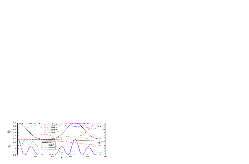
Figure 2: The revival probability $F(t)$ for various $c$.

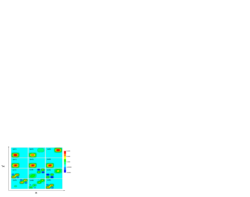
Figure 3: (Color online) Reduced single-particle density matrix $\rho(x,x^{\prime},t)$ of two interacting bosons for (a1-a3) $c=0,t=0,5,15$, (b1-b3) $c=5,t=0,5,15$, and (c1-c6) $c=\infty,t=0,5,16,21,22.5,32$. Each plot spans the range $-1<x,x^{\prime}<1$.

When the interaction is absent, bosons just oscillate back and forth between two wells and return to their initial state after a Rabi period $\tau$, which is the same as one boson’s. For interacting bosons, there will be many differences. The revival probability $F(t)$ as a function of time $t$ is shown in Fig.2 for various $c$. When interaction strength $c$ is very small, the revival probability $F(t)$ still displays the oscillating feature and the system returns to their initial state with probability close to $1$ after a longer period. The revival time becomes longer with the increase of the interaction strength $c$. When $c$ reaches a certain value ($c\sim 5$), $F(t)$ approaches $1$ with tiny oscillations within a very large time scale, which is known as the self trapping phenomena. In this regime, the tunneling to the right well is dynamically suppressed and two bosons stay in the left well stably. As the interaction strength $c$ increases further to the stronger regime, $F(t)$ begins to decrease more quickly and two bosons can tunnel to the right well again. In the limit of $c\rightarrow\infty$, $F(t)$ approaches zero quickly and then oscillates between $0$ and $0.521$, finally it approaches $1$ after almost a Rabi period. To see clearly how the atoms tunnel between the left and right wells, we display the corresponding time-dependent reduced single particle density matrix $\rho(x,x^{\prime},t)$ in Fig.3 for several typical $c$. The diagonal contribution $\rho(x,x^{\prime},t)$ along $x=x^{\prime}$ is just the single particle density distribution. In Fig.4, the pair correlation function $g^{(2)}(x_{1},x_{2},t)$ are also displayed. The pair correlation function $g^{(2)}(x_{1},x_{2},t)$ shows the probability of finding one particle at point $x_{1}$ and another particle at point $x_{2}$ in one measurement. As shown in $(a1)$, $(a2)$ and $(a3)$ of Fig.3 and Fig.4, the non-interacting bosons can tunnel from left well to right well, and then go back to left well, which forms a period of Rabi oscillation. However, as shown in $(b1)$-$(b3)$ of Fig.3 and Fig.4, the single particle density distribution and the pair correlation function $g^{(2)}(x,x^{\prime},t)$ have no obvious change within a Rabi period, and no oscillation between the left and right traps is observed in this self trapping regime with $c=5$. While in the fermionization limit, the oscillation phenomenon appears again in $(c1)-(c6)$. Both of two bosons tunnel to right well when $t=21$ (see $(c4)$) and go back to the left well for $t=32$ (see $(c6)$). Our results are consistent with results in Zollner based on the multi-configuration time-dependent Hartree method.

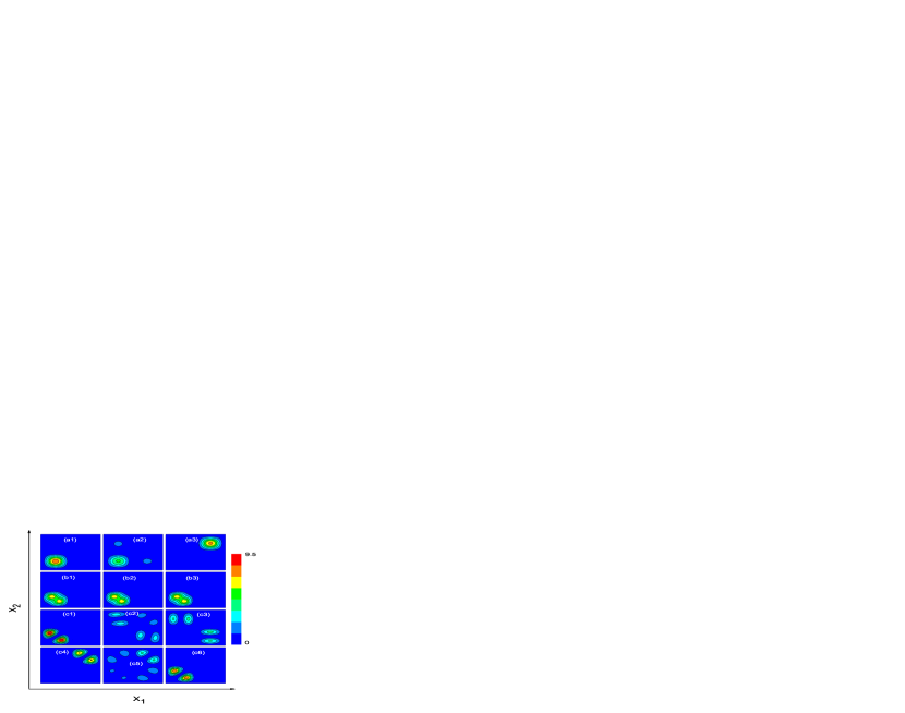
Figure 4: (Color online) The pair correlation function $g^{(2)}(x_{1},x_{2},t)$ for (a1-a3) $c=0,t=0,5,15$, (b1-b3) $c=5,t=0,5,15$, and (c1-c6) $c=\infty,t=0,5,16,21,22.5,32$. Each plot spans the range $-1<x,x^{\prime}<1$.

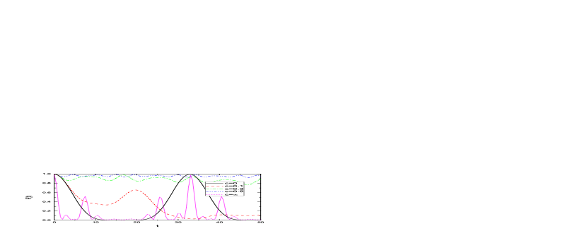
Figure 5: The revival probability $F(t)$ of three particles system changes with time $t$ with different interaction.

Next we consider the dynamics of systems with more bosons. The dynamics of $N=3$ system is similar to the $N=2$ case, except that the system enters self-trapping regime earlier than $N=2$. As shown in Fig. 5, when $c=0.5$, the system already displays the feature of self trapping with the fidelity $F(t)\sim 1$ with tiny oscillations within a very large time scale. Similarly, in the TG limit, bosons can tunnel to the right well more easy and return to the left well approximately after a Rabi period. The tunneling dynamics of hard-core bosons is very similar to their correspondence of free fermions Salasnich . In Fig.6, we plot the revival probability $F(t)$ for systems with $N=1$ to $N=4$ in the TG limit. It is shown that there is an obvious peak around the Rabi oscillation periods for various $N$, which implies that the system can return to the left well with probability close to $1$ after a Rabi period. One can understand this from the Bose-Fermi mapping, i.e., bosons in the TG limit can be mapped into a spinless free Fermi system Salasnich . For the case with $\kappa=50$, we can check that $J_{i}\approx i^{2}J_{1}$ for $i=1,2,3,4$. The $N$ atoms initially occupy the $N$-lowest single-particle levels of the left well, and roughly speaking, each particle tunnels with the Rabi period $\tau_{i}=-\pi/J_{i}$. However, when the particle number $N$ becomes large, the relations of $J_{i}\approx i^{2}J_{1}$ break down and even the dynamics in the TG limit can be quite complex.

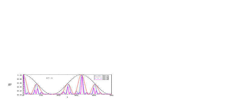
Figure 6: The revival probability $F(t)$ of the $N$-boson system changes with time $t$ with infinity interaction.

III.2 BHM approximation

Now we consider the two-site BHM described by the Hamiltonian (4). If the interaction strength is much smaller than the level spacing between the first band and the second band defined as $\Delta=\mu_{2}-\mu_{1}$, one may expect that the system can be approximately described by the single-band BHM. Under the one-band approximation, the Bose-Hubbard model is described by Eq.(6) with $i=1$. We note that the pair hopping term $U_{LR}^{1}$ in Eq.(6) is generally very small in comparison with the on-site interaction, for example, in the present work we have $U_{0}^{1}\approx 4948U_{LR}^{1}$. Therefore in many previous works, the pair hopping term is omitted and a simplified single-band BHM given by

$$\widehat{H} = \mu_{1}(n_{1,L}+n_{1,R})+\tilde{J_{1}}(a_{1,L}^{\dagger}a_{1,R}+a_{1,R}^{\dagger}a_{1,L})+$$ (12)

$$U_{0}^{1}[n_{1,L}(n_{1,L}-1)+n_{1,R}(n_{1,R}-1)],$$

has been widely used JPA381235 ; Ziegler ; BHM ; Wangli . Here $\tilde{J_{1}}=J_{1}+2(n_{1,L}+n_{1,R}-1)J^{\prime}_{1}$. Since $U_{LR}^{1}\ll U_{0}^{1}$ in the whole interacting regime, the pairing hopping term is not expected to significantly change the static properties. However, when the term $U_{LR}^{1}$ is comparable with the hopping amplitude $J_{1}$, it may give significant contribution to the dynamics, which has been emphasized in Ref.Liang . In the weakly interacting regime, the term of $J^{\prime}_{1}$ is also usually neglected as its revision to hopping energy can be attributed to $J_{1}$. As we shall illustrate later, when the interaction strength is very large, the contribution of $J^{\prime}_{1}$ can not be neglected since $J^{\prime}_{1}\propto c$.

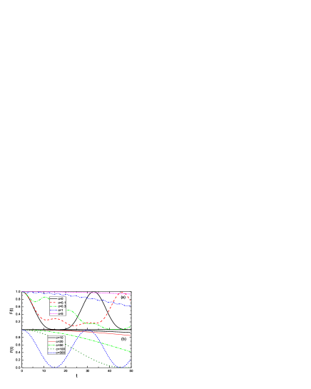
Figure 7: The revival probability $F(t)$ for the two-boson system changes with time $t$ under one-band BHM approximation.

By using the single-band BHM approximation, we study the tunneling dynamics of the two-site BHM described by $\widehat{H}_{1}$ given by Eq.(6) with all particles prepared in one site initially. The revival probability $F(t)$ changing with time $t$ under one-band BHM approximation are shown in Fig.7 for the two-boson system. As shown in Fig.7a, when the interaction strength is not very large, the single-band BHM gives quantitatively consistent description of the dynamics in comparison with the exact results by exact diagonalization (see Fig.2a). With further increase in the interaction, as shown in Fig.7b, although the single-band BHM with pairing hopping term can describe correctly the enhancement of tunneling, it does not provide quantitatively consistent results in comparison with results of exact diagonalization in Fig.2b. In order to see clearly the effect of the pair-tunneling term, we also study the dynamics governed by the simplified BHM of Eq.(12) without the pair-tunneling term. To see the effect of the term of $J^{\prime}_{1}$, we consider both cases for the Hamiltonian of Eq.(12) with or without the term of $J^{\prime}_{1}$. When the interaction strength is not so strong (for example, $c<5$), we find that the results are almost the same as that presented in Fig7a. That means that the terms of pair tunneling and $J^{\prime}_{1}$ are not important when the interaction is weak. However as shown in Fig.8 (a) and (b), the dynamics in the strongly interacting regime shows quite different behaviors if the pair tunneling term is absent. Comparing Fig.7b and Fig.8, we can conclude that the pair tunneling term of $U_{LR}^{1}$ gives an important contribution to tunneling in the large interaction regime. Comparing Fig.8a and Fig.8b, we find that the term of $J^{\prime}_{1}$ also plays an important role in enhancing the tunneling.

The dynamics for the three-boson system is shown in Fig.9. Comparing with the exact dynamical results in Fig.5, we find that the one-band BHM approximation can describe the dynamics well only when the interaction strength is small so that $U_{0}^{1}\ll\Delta$. In contrast to the two-boson system, the pair-tunneling term has less significant effect on the enhancement of the tunneling. For very large $c$, although the system can tunnel to the right well, it does not give quantitatively consistent results in comparison with results of the numerical exact diagonalization.

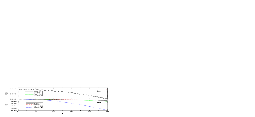
Figure 8: The revival probability $F(t)$ for the two-boson system changes with time $t$ under one-band BHM approximation with (a) $U_{LR}^{1}=0$ and $J^{\prime}_{1}=0$. (b) $U_{LR}^{1}=0$.

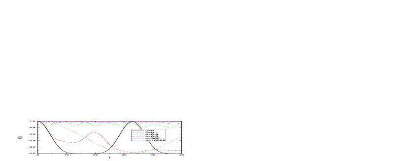
Figure 9: The revival probability $F(t)$ for the three-boson system changes with time $t$ under one-band BHM approximation.

From the above results, we know that one-band BHM approximation is not enough to give a quantitatively description for the dynamics of interacting bosons in the large interaction regime. To get better results, we need keep more band levels and use the multi-band BHM given by Eq.(4) in our calculation. In Fig.10, we show the ground energy of the two bosons versus the interaction strength using exact diagonalization method, one-band, two-band, three-band and four-band BHM approximations, respectively. It is shown that one-band BHM approximation can describe the ground energy very well when the interaction $c<1$, and two-band BHM approximation can describe well in the region $c<10$, while three-band and four-band BHM approximations are efficient to describe the ground energy of two bosons well even for $c=100$. For the dynamics problem, in order to get a quantitatively consistent results with the exact diagonaliztion results, we find that more bands are needed in comparison with the static problem. In Fig.11, we display the results of $F(t)$ for the two-particle systems with various $c$ within the multi-band BHM approximation. As shown in the figure, the result based on a five-band BHM approximation for $c=10$ already quantitatively agrees with the exact numerical result. For $c=50$, a ten-band BHM approximation is required for a quantitatively consistent result. The result for $c=300$ based on an eighteen-band BHM approximation is also given in Fig.11. In comparison with Fig.2b and Fig.7b, we find that there exists only a qualitative agreement with the exact diagonaliztion result although it is much better than the result of the single-band BHM approximation.

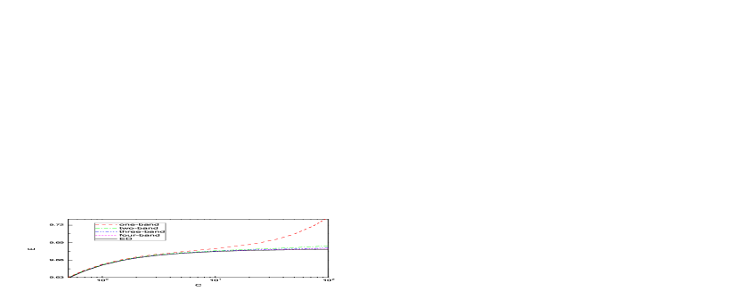
Figure 10: The ground energy for the two-boson system obtained by exact diagonalization method and $i$-band BHM approximation with $i=1,2,3,4$.

Figure 11: The revival probability $F(t)$ changes with time $t$ under multi-band BHM approximations, including a five-band BHM approximation for $c=10$, a seven-band BHM approximation for $c=20$, a ten-band BHM approximation for $c=50$ and a eignteen-band BHM approximation for $c=300$.

IV Summary

In summary, we have studied the dynamical properties of a few bosons confined in an one-dimensional split hard wall trap by both the exact diagonaliztion method and the approximate method based on the two-site Bose-Hubbard model. The system is initially prepared in the left well of the trap by setting the barrier strength of the split hard wall trap to infinity, and then it is suddenly changed to a finite value. With the increase in the interaction strength of bosons, the system displays the Josephson-like oscillations, self trapping and correlated tunneling in turn. Comparing results obtained by two different methods, we conclude that the one-band BHM approximation can quantitatively describe the dynamics in the weakly interacting regime, but the multi-band BHM approximation is needed if we want to describe the dynamics of bosons with large interaction quantitatively. We also validate that the form of correlated tunneling gives an important contribution to the tunneling dynamics in the large interaction regime.

References

- (1) A. Smerzi, S. Fantoni, S. Giovanazzi, and S. R. Shenoy, Phys. Rev. Lett. 79, 4950 (1997).
- (2) G. J. Milburn, J. Corney, E. M. Wright, and D. F. Walls, Phys. Rev. A 55, 4318 (1997).
- (3) S. Raghavan, A. Smerzi, S. Fantoni, and S. R. Shenoy, Phys. Rev. A 59, 620 (1999).
- (4) A. J. Leggett, Rev. Mod. Phys. 73, 307 (2001).
- (5) R. W. Spekkens and J. E. Sipe, Phys. Rev. A 59, 3868 (1999).
- (6) G. F. Wang, L. B. Fu, and J. Liu, Phys. Rev. A 73, 013619 (2006).
- (7) K. W. Mahmud, H. Perry, and W. Reinhardt, Phys. Rev. A 71, 023615 (2005).
- (8) A. P. Tonel, J. Links, and A. Foerster, J. Phys. A 38, 1235 (2005).
- (9) J. Goold, and Th. Busch, Phys. Rev. A 77, 063601 (2008); D. S. Murphy, J. F. McCann, J. Goold and Th. Busch, Phys. Rev. A 76, 053616 (2007).
- (10) X. Yin, Y. Hao, S. Chen, and Y. Zhang, Phys. Rev. A 78, 013604 (2008).
- (11) I. Bloch, J. Dalibard, and W. Zwerger, Rev. Mod. Phys. 80, 885 (2008); C. Chin, R. Grimm, P. Julienne, and E. Tiesinga, Rev. Mod. Phys. 82, 1225 (2010).
- (12) S. Fölling et al., Nature (London) 448, 1029 (2007).
- (13) S. Zöllner, H.-D. Meyer, P. Schmelcher,Phys. Rev. Lett. 100, 040401 (2008); Phys. Rev. A 78, 013621 (2008).
- (14) J.-Q. Liang, J.-L. Liu, W.-D. Li, and Z.-J. Li, Phys. Rev. A 79, 033617 (2009).
- (15) K. Sakmann, A. I. Streltsov, O. E. Alon, and L. S. Cederbaum, Phys. Rev. Lett. 103, 220601 (2009).
- (16) M. Albiez, R. Gati, J. Folling, S. Hunsmann, M. Cristiani, and M. K. Oberthaler, Phys. Rev. Lett. 95, 010402 (2005).
- (17) B. Paredes, A. Widera, V. Murg, O. Mandel, S. Fölling, I. Cirac, G. V. Shlyapnikov, T. W. Hänsch, and I. Bloch, Nature 429, 277 (2004).
- (18) T. Kinoshita, T. Wenger and D. S. Weiss, Science 305, 1125 (2004).
- (19) M. D. Girardeau, J. Math. Phys. (N.Y.) 1, 516 (1960); Phys. Rev. 139, B500 (1965).
- (20) Y. Hao, Y. Zhang, J. Q. Liang and S. Chen, Phys. Rev. A. 73, 053605 (2006).
- (21) F. Deuretzbacher, K. Bongs, K. Sengstock, and D. Pfannkuche, Phys. Rev. A 75, 013614 (2007).
- (22) Y. Hao and S. Chen, Eur. Phys. J. D 51, 261 (2009).
- (23) S. Zöllner, H.-D. Meyer, and P. Schmelcher, Phys. Rev. A 74, 063611 (2006); Phys. Rev. A 74, 053612 (2006).
- (24) O. E. Alon, and L. S. Cederbaum, Phys. Rev. Lett. 95, 140402 (2005).
- (25) M. P. A. Fisher, P. B.Weichman, G. Grinstein, and D. S. Fisher, Phys. Rev. B 40, 546 (1989); D. Jaksch, C. Bruder, J. I. Cirac, C. W. Gardiner, and P. Zoller, Phys. Rev. Lett. 81, 3108 (1998).
- (26) L. Wang, Y. Hao and S. Chen, Phys. Rev. A 81, 063637 (2010); Eur. Phys. J. D 48, 229 (2008).
- (27) K. Ziegler, Phys. Rev. A 81, 034701 (2010).
- (28) L. Salasnich, G. Mazzarella, M. Salerno, and F. Toigo, Phys. Rev. A 81, 023614 (2010).