Quantum noise in ac-driven resonant-tunneling double barrier structures: Photon-assisted tunneling vs. electron anti-bunching

Abstract

We study the quantum noise of electronic current in a double barrier system with a single resonant level. In the framework of the Landauer formalism we treat the double barrier as a quantum coherent scattering region that can exchange photons with a coupled electric field, e.g. a laser beam or a periodic ac-bias voltage. As a consequence of the manyfold parameters that are involved in this system, a complicated step-like structure arises in the non-symmetrized current-current auto correlation spectrum and a peak-like structure in the cross correlation spectrum with and without harmonic ac-driving. We present an analytic solution for these noise spectral functions by assuming a Breit-Wigner lineshape. In detail we study how the correlation functions are affected by photo-assisted tunneling (PAT) events and discuss the underlying elementary events of charge transfer where we identify a new kind of contribution to shot-noise. This enables us to clarify the influence of a not centered irradiation of such a structure with light in terms of contributions originating from different sets of coherent scattering channels. Moreover we show how the noise is influenced by acquiring a scattering phase due to the complex reflection amplitudes that are crucial in the Landauer approach.

I Introduction

As a striking consequence of charge quantisation shot noise can be used to characterize electron transport in mesoscopic systems LevitovLesovik93 ; BlanterButtiker00 ; Schonenberger03 ; Nazarov03 . In ballistic electron transportWharam88 ; vanWees88 partitioning of the scattered quasiparticles Buettiker94 is the mechanism defining the statistics of charge fluctuations in the two leads. Indeed, the principle of counting individual charges leads to the full counting statistics approach LevitovLee96 which has been successfully applied to tackle a variety of problems, e. g. superconducting heterostructures Belzig01a ; Belzig01b , electron transport in multi-terminal conductors Nazarov02 , zero-frequency noise in multi-level quantum dots Belzig05 or frequency-dependent noise in interacting conductors. Emary07 This formalism has also been incorporated to characterize the elementary events of current-current correlations for energy-independent scattering at zero frequency but with finite ac-driving voltage. VanevicBelzig07 ; VanevicBelzig08 Such an harmonic voltage dependence can be induced by irradiating the structure with light PedersenButtiker98 , e.g a laser beam. Erbe06 Ongoing effort in improving the detection of current-current correlations at high frequencies Gabelli08 ; Gabelli09 ; ZakkaBajjani10 and coupling such structures to light fields or ac-bias voltages Grifoni98 ; LesovikLevitov94 ; Brune97 ; Schoelkopf97 ; Moskalets02 ; Kohler05 ; Moskalets08 offers an interesting playground to examine quantum charge transport or light-matter interaction in mesoscopic systems. Within the last years considerable progress in ac-transport has been achieved. E.g. the irradiation induced opening of a dynamical gap has been calculated Fistul07 in a 2D electron gas when spin-orbit interaction is present. The current and noise through long, ac-driven molecular wires Camalet04 ; Kaiser07 ; Safi08 ; Safi09 , various aspects about ac-driven carbon based conductors Trauzettel07 ; Fistul07b ; Syzranov08 ; Zeb08 ; Rocha10 , photo-assisted noise in the fractional quantum Hall regime Crepieux04 , low-frequency current noise in diffusive conductors Bagrets07 , noise in adiabatic pumping Moskalets04 ; Moskalets06 ; Moskalets07 and the influence of electron-phonon interaction has been studied Aguado04 . Even more works have investigated the influence of Coulomb repulsion on the transport through a quantum dot Sukhorukov01 ; Dong04 ; Djuric05 ; Thielmann05a ; Thielmann05 ; Braun06 ; Dong08 . Electron-electron interactions can be included within a Green function formalism or generalized master-equation approach. Interestingly, quantum noise spectra are symmetrized by performing a Markov approximation Engel03 ; EngelLoss04 . In this classical limit, one can make use of the Mac Donald formula and calculate the noise of a quantum dot system with ac-bias voltages up to a Born approximation as shown recently in Ref. Wu10 .

It has been shown recently in experiment Gabelli08 ; Gabelli09 ; ZakkaBajjani10 ; Glattli09 ; Reydellet03 ; Reulet03 and theoretically Lesovik97 ; GavishImry00 ; GavishImry01 ; Beenakker01 ; Schonenberger03 ; Engel03 ; EngelLoss04 ; EntinWohlman07 ; Rothstein08 ; Nazarov03 that the noise of a two-terminal device, as for a coherent scattering double barrier structure, leads to an asymmetric noise spectrum in the quantum regime. Since current operators at different times do not commute one could argue that, in order to get physical results, the shot-noise spectrum should be symmetrized in the frequency $\Omega$ in analogy to the classical noise PedersenButtiker98 . Indeed, such a quantity describes experiments in the classical detection regime correctly Lesovik97 ; Bednorz08 ; Bayandin08 ; Bednorz10 ; Bednorz10a . Nevertheless it has become clear during the last years that asymmetric noise can be measured if a detector discriminates between the absorption and emission of energy quanta $\hbar\Omega$ from or to the system GavishImry00 ; GavishImry01 . Then the positive (negative) frequencies of the noise spectra correspond to energy quanta $\hbar\Omega$ transferred from (to) the radiation field to (from) the charge carriers in the quantum dot. The negative frequency part of the spectrum, the emission branch, should be measured by an active detector setupGavishImry01 , since at low enough temperature the energy transfer from the quasiparticles to the radiation field is forbidden otherwise. The detected current fluctuations are described by a combination of the “pure” correlators of two currents at different times. Fourier transformation to the frequency domain defines the asymmetric noise spectrum, which might in addition depend on some harmonic driving in the leads $eV_{ac}\cos(\omega t)$, as

$$S_{\alpha\beta}(\Omega,\Omega^{\prime},\omega)=\int\limits_{-\infty}^{\infty}dtdt^{\prime}S_{\alpha\beta}(t,t^{\prime},\omega)e^{i\Omega t+i\Omega^{\prime}t^{\prime}}\,.$$ (1)

The non-symmetrized shot noise correlates currents at two times:

$$S_{\alpha\beta}(t,t^{\prime},\omega)=\left\langle\Delta\hat{I}_{\alpha}(t)\Delta\hat{I}_{\beta}(t^{\prime})\right\rangle$$ (2)

with variance $\Delta\hat{I}_{\alpha}(t)=\hat{I}_{\alpha}(t)-\langle\hat{I}_{\alpha}(t)\rangle$. Experimental accessible are the fluctuations averaged over a timescales large compared to the one defined by the driving frequency $\omega$. Thus, as in Ref. PedersenButtiker98 , we introduce Wigner coordinates $t=T+\tau/2$ and $t^{\prime}=T-\tau/2$ and average over a driving period $2\pi/\omega$. Then the noise spectrum is defined by the quantum statistical expectation value of the Fourier-transformed current-operator $\hat{I}_{\alpha}(\Omega)$ via $S_{\alpha\beta}(\Omega,\Omega^{\prime},\omega)=2\pi\delta(\Omega+\Omega^{\prime})S_{\alpha\beta}(\Omega,\omega)=\langle\hat{I}_{\alpha}(\Omega)\hat{I}_{\beta}(\Omega^{\prime})\rangle$. $S_{\alpha\beta}(\Omega,\omega)$ is just the Fourier transform of $S_{\alpha\beta}(\tau,\omega)$. Similarly, in the case without ac-driving the noise is only a function of relative times $\tau=t-t^{\prime}$. In order to keep notation short, in the dc-bias limit we write $S_{\alpha\beta}(\Omega):=S_{\alpha\beta}(\Omega,\omega=0)$.

As we show in this article, the finite frequency current noise can be interpreted by splitting it into contributions which are emanating from reservoir $\alpha={L,R}$ and being scattered into terminal $\beta=L,R$. This motivates us to study the individual auto-terminal and cross-terminal current-current correlators, the ‘building-blocks’ of the possible noise spectra measured in experiments Schonenberger03 ; Reulet03 ; Reydellet03 ; Gabelli08 ; Glattli09 ; Gabelli09 ; ZakkaBajjani10 . The paper is organized as follows: Below we describe the basic properties of the driven quantum dot. In the next section we provide the basic formulas in the scattering formalism. The main results are discussed in the two following parts about the auto- and cross-correlation noise spectra. We relate features of the calculated plots to possible scattering events and compare the spontaneous PAT events at finite dc-bias without driving with those induced by the ac-voltage. Where possible we connect our approach to known cases. The following part is devoted to interpret the results in terms of elementary events of charge transfer. The results are summarized in the last section of this article.

For resonant tunneling with energy-dependent transmission through the scattering region, e.g. as in many quantum dots or molecules, the scattered particles have to be in resonance with the available energy levels of the scatterer. In case of a single resonant level at least one of the chemical potentials of the reservoirs has to be aligned with this energy level. Alternatively a quasiparticle in the leads has to absorb or emit suitable energy quanta to bridge the energy gap between the chemical potential and the resonance. This can be achieved via absorption or emission of photons stimulated by an external electric field, typically a microwave or laser beam. In the Tien-Gordon theory TienGordon62 ; PedersenButtiker98 such an illumination with light corresponds to an oscillating voltage in either one or both leads. Depending on the way the light field is coupled to the electronic circuit it has to be treated as either symmetric or asymmetric in the amplitudes of the harmonic ac-driving in the left and right lead. A spatial asymmetry in the illumination could additionally introduce different temperatures in the two leads and thus create thermo-currents Moskalets02 . If the driving is asymmetric there can be a photocurrent even when no bias voltage is applied. For the noise, asymmetry effects in terms of enhancement or reduction of the ac-drive in a terminal $\alpha$ can be related to the corresponding correlator and so to the kind of scattering events described by its integrand. We neglect interactions and disregard charging effects by assuming metallic structures with pefect screening. In general one should treat charging effects in a self-consistent manner via a dynamical conductancePedersenButtiker98 ; ButtikerPretre93 ; ButtikerChristen96 ; ChristenButtiker96 , which has been recently confirmed experimentally Gabelli07

II Scattering approach to resonant tunneling with ac-driving

Following the work of Pedersen and Büttiker PedersenButtiker98 we take the ac-voltage $V_{m}(t)=V_{ac,{m}}\cos\left(\omega t\right)$ at contact $m=L,R$ into account by redefinition of the reservoir operators via $\hat{a}_{m}(\epsilon)=\sum_{l}\hat{a}^{\prime}_{m}(\epsilon-l\hbar\omega)J_{l}\left(\alpha_{m}\right)$.

Figure 1: Top: Zero-temperature auto-correlations for a centered resonance (top) where each curve belongs to a different resonance width $\gamma$. The curves are for symmetrically applied dc-bias ($-eV/2=\mu_{l}=-\mu_{r}$). With increasing resonance width $\gamma$ the step-like structure of the noise spectrum gets washed out. By increasing $\gamma$ the noise at negative frequencies is reduced while the spectrum exhibits the typical linear frequency-dependence for energy-independent scattering. Bottom: The four contributions to the noise spectrum $S_{LL}(\Omega,L)_{\alpha\rightarrow\beta}$ for resonance positions $\epsilon_{r}/eV=-0.3,0,0.3$ and $\gamma/eV=0.01$ are shown. Shifting the resonance or the potentials will change the positions of the steps and the impact of the contributions.

Here the $J_{l}$ are the Bessel functions of the first kind. The dimensionless parameters $\alpha_{L}=\frac{a+1}{2}\alpha$ and $\alpha_{R}=\frac{a-1}{2}\alpha$ define the strength of the ac-drive in the contacts via $\alpha=\frac{eV_{ac}}{\hbar\omega}$ and the asymmetry parameter $a\in[-1,1]$. $V_{ac}$ denotes the amplitude of the ac-bias coupling to the DB system and $\omega$ the corresponding driving frequency. In order to write down the current one has to integrate the expression for the current operator and replace the statistical averages of the creation and annihilation operators by their equilibrium values. For the Fermi function in lead $m$ the abbreviation $f^{\mathrm{e}}_{m}(\epsilon)=\left[\exp\left(\beta_{m}(\epsilon-\mu_{m})\right)+1\right]^{-1}$ with $\beta_{m}=1/(k_{B}\mathcal{T}_{m})$ is used. Unoccupied states, in other words occupied hole-like states, are denoted by $f^{\mathrm{h}}_{m}(\epsilon)=1-f^{\mathrm{e}}_{m}(\epsilon)$.
We treat our setup as a Fabry-Pérot like DB system, for which the transmission probability $T(\epsilon,\epsilon_{r})=t^{\dagger}(\epsilon,\epsilon_{r})t(\epsilon,\epsilon_{r})$ is well known Datta . Incoming and outgoing scattering states are related by the energy-dependent scattering matrix (s-matrix) via $\hat{b}_{n}(\epsilon)=\sum_{m}s_{mn}\hat{a}_{m}(\epsilon)$. The s-matrix is of the form

$$s(\epsilon,\epsilon_{r})=\left(\begin{array}[]{cc}r(\epsilon,\epsilon_{r})&t^{\prime}(\epsilon,\epsilon_{r})\\ t(\epsilon,\epsilon_{r})&r^{\prime}(\epsilon,\epsilon_{r})\end{array}\right)\,.$$ (3)

For a resonant level we can use the Breit-Wigner expression to define the matrix elements and thus the transmission through the scattering region via

$$s_{mn}(\epsilon,\epsilon_{r})=\delta_{mn}-i\frac{\sqrt{\gamma_{m}\gamma_{n}}}{\epsilon-\epsilon_{r}+i\frac{\gamma}{2}}\;\text{,}$$ (4)

where $\gamma=\sum_{m}\gamma_{m}$ is the half width of the resonance and $\epsilon_{r}$ is the resonance energy of the level. In general the barrier strength $\gamma_{n}$ could also depend on energy which we neglect here for simplicity. Furthermore we assume symmetric barriers $\gamma_{L}=\gamma_{R}=\gamma/2$ and call the setup symmetric if the resonance is at the Fermi energy ($\epsilon_{r}=0)$ and $-\mu_{L}=\mu_{R}=eV/2$.

If the s-matrix does not dependent on energy, quantum-noise generated by the current partitioning at the scattering region can be traced down to fluctuations in the electronic occupations of the contact with the emission of carriers from left and right leads MartinLandauer92 . These fluctuations are the sum of variances of the possible current pulses of incident (or empty) wave packets at left and right contacts times their weight factors. An incident wave packet can either be transmitted, with probability $T$, or reflected with probability $1-T$. It has been shown that in this limit completely closed ($T=0$) or open ($T=1$) channels can not produce any noise, since either no charge is transferred or their is no partitioning at the scatterer. For intermediate values of $T$ the quantum noise in this regime consists of four linear contributions. Two contribution with initial and final states related to the same terminal with onsets at $\Omega=0$ and two contributions with initial and final states at opposite terminals and onsets at $\hbar\Omega=\pm eV$. This limit is approached in the spectrum of Fig. 1 for $\gamma\gtrsim eV$. Thus, at zero temperature the asymmetric noise spectrum is nonzero if $\hbar\Omega>-eV$ and exhibits kinks at frequencies $\hbar\Omega=0,eV$. When performing the zero-frequency limit some contributions will be absent due to Pauli principle. This is e.g the case for current pulses incident from right and left lead where one is transmitted and the other one reflected, the whole process being proportional to $T(1-T)f^{\mathrm{e}}_{\alpha}(\epsilon)f^{\mathrm{e}}_{\beta}(\epsilon)$, because then $f^{\mathrm{e}}_{\alpha}(\epsilon)=f^{\mathrm{e}}_{\beta}(\epsilon)$. However, at finite frequency and with additional ac-driving it is in general not possible to express the noise in terms of transmission or reflection probabilities but one has to interpret the different products of s-matrices involved in the four contributions to the noise. The weight of these contributions is given by the Besselfunctions $J_{n}\left(\alpha\right)$ that describe a photon emission or absorption processes of order $n$ at driving strength $\alpha$. The noise spectral density is defined as

$$S_{\alpha\beta}(\Omega,\omega)=\left(\frac{e^{2}}{2\pi\hbar}\right)\int d\epsilon\underset{\gamma\delta,lkm}{\sum}J_{l}\left(\frac{eV_{\gamma}}{\hbar\omega}\right)J_{k}\left(\frac{eV_{\delta}}{\hbar\omega}\right)J_{m+k-l}\left(\frac{eV_{\delta}}{\hbar\omega}\right)J_{m}\left(\frac{eV_{\gamma}}{\hbar\omega}\right)$$

$$Tr\left[{\bf A}_{\gamma\delta}(\alpha,\epsilon,\epsilon+\hbar\Omega){\bf A}_{\delta\gamma}(\beta,\epsilon+\hbar\Omega+(m-l)\hbar\omega,\epsilon+(m-l)\hbar\omega,)\right]f^{\mathrm{e}}_{{\gamma}}(\epsilon-l\hbar\omega)f^{\mathrm{h}}_{{\delta}}(\epsilon+\hbar\Omega-k\hbar\omega)$$ (5)

With the so-called current matrix ${\bf A}_{\gamma\delta}(\alpha,\epsilon,\epsilon^{\prime})=\delta_{\alpha\gamma}\delta_{\beta\delta}-s^{*}_{\alpha\gamma}(\epsilon)s_{\beta\delta}(\epsilon^{\prime})$ which connects incoming and outgoing states via the s-matrices at different energies.

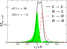
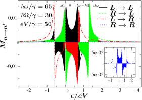
Figure 2: Examples of the integrands real parts for finite $eV$ without (top) and with (bottom) ac-driving. We show the integrands $M_{n\rightarrow n^{\prime}}(\Omega,\omega)$ with $(n,n^{\prime})=$ (L,L), (L,R), (R,L) and (R,R) as a function of $\epsilon$ for a centered resonance ($\epsilon_{r}=0$). The lines show the integrand while the filling denotes the integration interval. Top: No ac-driving, so at negative frequency only $R\rightarrow L$ contributions are present, as indicated by the shaded region. The $L\rightarrow R$ term is similar to the other cross-terminal contribution, both have a single peak, located at $\epsilon=\epsilon_{r}$ or at $\epsilon=\epsilon_{r}-\hbar\Omega$. If $\Omega\rightarrow 0$ these terms interfere destructively leading to a double peak shape with maximal values of $1/4$ around the local minima at $\epsilon=0,-\hbar\Omega$. The auto-terminal contributions have a double-peak structure at the same energies. For $\Omega \rightarrow 0$ the $L\rightarrow L$ term can be $>1$, but it is not probed for a centered resonance. Its significant contributions are at $\hbar\Omega\geq eV/2$ and not shown in the example. Bottom: Integrands of the ac-driven setup with $\hbar\Omega/\gamma=30$, $\hbar\omega/\gamma=65$, and $l=1$; other parameters as above. Due to the complex s-matrices negative values are possible.

If one of the frequencies involved is zero at least some correlators can be written in terms of $T(\epsilon)$ and $R(\epsilon)$. But in general this is not the case due to the special role of the complex reflection amplitudes. In equilibrium ($eV=0,\alpha=0$) these amplitudes lead to finite noise even if no transmission through the system is possible Buttiker92 . We will emphasize their special role concerning the noise spectral function if finite bias voltages are applied. Therefore we separate the dc-noise spectrum into a sum of states which are scattered from terminal $\alpha$ to terminal $\beta$:

$$S_{LL}(\Omega,\omega):=\underset{\alpha,\beta=L,R}{\sum}C^{\mathrm{}}_{\alpha\rightarrow\beta}(\Omega,\omega)$$ (6)

The four correlators contributing to auto-correlation noise without time-dependent voltages ($\omega=0$) are then determined by

$$C^{\mathrm{}}_{L\rightarrow L}(\Omega)= \frac{e^{2}}{2\pi\hbar}\Theta(\hbar\Omega)\underset{\mu_{L}-\hbar\Omega}{\overset{\mu_{L}}{\int}}d\epsilon\,\left|r^{*}(\epsilon)r(\epsilon+\hbar\Omega)-1\right|^{2}$$ (7a)

$$C^{\mathrm{}}_{R\rightarrow R}(\Omega)= \frac{e^{2}}{2\pi\hbar}\Theta(\hbar\Omega)\underset{\mu_{R}-\hbar\Omega}{\overset{\mu_{R}}{\int}}d\epsilon\,T(\epsilon)T(\epsilon+\hbar\Omega)$$ (7b)

$$C^{\mathrm{}}_{L\rightarrow R}(\Omega)= \frac{e^{2}}{2\pi\hbar}\Theta(\hbar\Omega-eV)\underset{\mu_{R}-\hbar\Omega}{\overset{\mu_{L}}{\int}}d\epsilon\,R(\epsilon)T(\epsilon+\hbar\Omega)$$ (7c)

$$C^{\mathrm{}}_{R\rightarrow L}(\Omega)= \frac{e^{2}}{2\pi\hbar}\Theta(\hbar\Omega+eV)\underset{\mu_{L}-\hbar\Omega}{\overset{\mu_{R}}{\int}}d\epsilon\,T(\epsilon)R(\epsilon+\hbar\Omega)\,.$$ (7d)

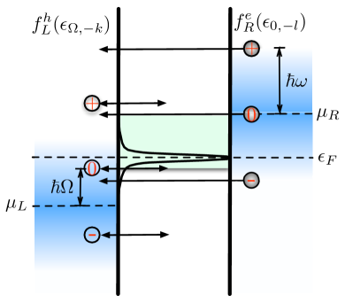
Figure 3: Elementary events of $C^{\mathrm{}}_{\alpha\rightarrow\beta}(\Omega,\omega)$. We have chosen $(\alpha,\beta)=$ (R,L) and $\epsilon_{r}=0$ as an example. The frequency is fixed close to the step at $\hbar\Omega=-eV/2$ in the noise spectrum. A higher frequency would shift the lower bound of the integration window (colored region around the resonance) and the hole-like final states downward towards $\mu_{L}$. The filling of the left and right reservoirs refer to the applied dc- and ac-bias voltages. The available free and occupied states are defined by the Fermi functions for electrons $f^{\text{e}}_{L/R}(\epsilon_{\Omega},k)=f_{L/R}(\epsilon+\hbar\Omega+k\hbar\omega)$ and for holes $f_{L/R}^{\text{h}}(\epsilon_{\Omega},k)=1-f_{L/R}(\epsilon+\hbar\Omega+k\hbar\omega)$. Arrows indicate the possible mechanism which are suggested by the products of s-matrices that appear in the integrands. We show the contributions up to first order in the driving $n\hbar\omega$, so $n=0,\pm 1$. The colored region in-between the barriers denotes the integration interval when n=0.

Here the correlator of Eqn. (7a) can not explicitly be written as a product of probabilities. Rather we find a term with states scattered from and back to lead $L$ describing the two-particle quantum interference of coherently scattered quasiparticles with the occupied states in the lead where current-fluctuations are measured. The quasiparticles in the lead can interfere with either a reflected quasi-electron that absorbs a quanta $\hbar\Omega$ or with a quasi-hole propagating along the inverse path and emitting a photon with energy $\hbar\Omega$. In terms of probabilities $C^{\mathrm{}}_{L\rightarrow L}(\Omega)$ acquires a finite scattering-phase $\Phi(\epsilon,\Omega)=\text{Arg}\left[r^{*}(\epsilon)r(\epsilon+\Omega)\right]$ via its integrand that can be written as $(1+R(\epsilon)R(\epsilon+\hbar\Omega)-2[R(\epsilon)R(\epsilon+\hbar\Omega)]^{1/2}\cos(\Phi(\epsilon,\Omega)))f^{\mathrm{e}}_{L}(\epsilon)f^{\mathrm{h}}_{L}(\epsilon+\hbar\Omega)$. Moreover it is this contribution that can produce noise even for vanishing transmission, in analogy to the equilibrium problem. For our choice of chemical potentials the only non-vanishing correlator at zero-frequency is given by Eq. (7d).

Without ac-bias voltages but at finite frequency the auto-correlations are real and the cross-correlations at opposite terminals are the hermitian conjugate of each other, so they obey the symmetries:

$$S^{\dagger}_{LL}(\Omega) =S_{LL}(\Omega)$$ (8)

$$S^{\dagger}_{LR}(\Omega) =S_{RL}(\Omega)$$ (9)

In addition, if $\Omega=0$, the well-known symmetry $S_{\alpha\alpha}(\Omega=0)=-S_{\alpha\beta}(\Omega=0)$ is recovered, so the sum of all current-correlations vanishes $\sum\limits_{\alpha,\beta=L,R}S_{\alpha\beta}(\Omega=0)=0$, see also Refs. BlanterButtiker00 ; Rothstein08 . In order to develop an intuitive interpretation for products of two s-matrices $s^{*}_{\alpha\beta}(\epsilon)s_{\alpha^{\prime}\beta^{\prime}}(\epsilon+\hbar\Omega)$ we express them in terms of probabilities. If both s-matrices have the same indices $\alpha^{\prime}=\alpha$ and $\beta^{\prime}=\beta$ we introduce the transmission and reflection functions

$$T(\epsilon,\epsilon+\hbar\Omega) =t^{*}(\epsilon)t(\epsilon+\hbar\Omega)$$ (10)

$$R(\epsilon,\epsilon+\hbar\Omega) =r^{*}(\epsilon)r(\epsilon+\hbar\Omega)\,.$$ (11)

In terms of the usual probabilities $T(\epsilon)$ and $R(\epsilon)$ we find

$$T(\epsilon,\epsilon+\hbar\Omega)=$$

$$T(\epsilon)\left(\frac{\epsilon+\hbar\Omega\,T(\epsilon+\hbar\Omega)}{\epsilon+\hbar\Omega}+\frac{i\hbar\Omega\,T(\epsilon+\hbar\Omega)}{\gamma}\right)$$ (12)

$$R(\epsilon,\epsilon+\hbar\Omega)=$$

$$R(\epsilon)\left(\frac{\epsilon+\hbar\Omega\,T(\epsilon+\hbar\Omega)}{\epsilon}+\frac{i\hbar\Omega(\epsilon+\hbar\Omega)T(\epsilon+\hbar\Omega)}{\epsilon\gamma}\right)\,.$$ (13)

For $\Omega\rightarrow 0$ these expressions reproduce the probabilities $T(\epsilon)$ and $R(\epsilon)$. At finite $\Omega$ they illustrate nicely how an imaginary part and at the same time an additional contribution to the real part are acquired, both proportional to $\hbar\Omega\,T(\epsilon+\hbar\Omega)$. At the same time contributions proportional to the probability $T(\epsilon)$ are modified by a factor $\epsilon/(\epsilon+\hbar\Omega)$. Depending on the value of $\Omega$ this can lead to a reduced or enhanced transmission function for those processes. The imaginary part can be seen as a finite scattering time in the FP setup where the corresponding timescale is given by the inverse resonance width $1/\gamma$. If we allow arbitrary pairings of s-matrices at energies separated by the frequencies $\Omega,\omega$, as they appear in in Eq. (5) for the noise spectral function with finite ac-bias voltage, we find the transmission functions

$$T(\Omega_{m},\omega_{n}):=s^{*}_{LR}(\Omega_{m})s_{LR}(\omega_{n})$$

$$=T(\Omega_{m})T(\omega_{n})\left(1+\frac{\epsilon_{m}\epsilon_{n}}{\gamma^{2}}+i\frac{\omega_{n}-\Omega_{m}}{\gamma}\right)$$ (14a)

$$R(\Omega_{m},\omega_{n}):=s^{*}_{LL}(\Omega_{m})s_{LL}(\omega_{n})$$

$$=R(\epsilon_{m})R(\epsilon_{n})\left(1+\frac{\gamma^{2}}{\epsilon_{m}\epsilon_{n}}+i\frac{\gamma(\omega_{n}-\Omega_{m})}{\epsilon_{n}\epsilon_{m}}\right)$$ (14b)

$$M(\Omega_{m},\omega_{n}):=s^{*}_{LL}(\Omega_{m})s_{LR}(\omega_{n})$$

$$=R(\Omega_{m})T(\omega_{n})\left(\frac{\omega_{n}-\Omega_{m}}{\epsilon_{n}}+i\frac{\epsilon^{2}_{n}+\gamma^{2}}{\gamma\epsilon_{n}}\,.\right)$$ (14c)

Above we used the shorthands $$\omega_{m}(\Omega_{m})=m\hbar\omega(\Omega) \epsilon_{n(m)}=\epsilon+\omega_{n}(\Omega_{m}) m,n$$ and , with integer .

Since we only regard symmetric coupling to the leads ($\gamma_{L}=\gamma_{R}$) the s-matrices are invariant when exchanging reservoir indices $L$ and $R$. Then the noise is symmetric under exchange of the indices $L,R$ if the dc-bias is reversed, too. Therefore we only deal with the auto-correlation and cross-correlation noise $S_{LL}(\Omega,\omega)$ and $S_{LR}(\Omega,\omega)$. Consequently we also give the formulas in terms of $t(\epsilon)=s_{LR}(\epsilon)=s_{RL}(\epsilon)$ as well as $r(\epsilon)=s_{LL}(\epsilon)=s_{RR}(\epsilon)$.

III Current-current auto correlations

The description in terms of initial and final states defined by the Fermi function products is supported by expressing the noise spectrum with the help of Fermi’s golden rule GavishImry00 ; GavishImry01 :

$$S_{\alpha\alpha}(\Omega)=2\pi\underset{\mathrm{i,f}}{\sum}P_{\mathrm{i}}\left|\left<\mathrm{i}\left|\Delta\hat{I}_{\alpha}\right|\mathrm{f}\right>\right|^{2}\delta\left(\epsilon_{\mathrm{i}}-\epsilon_{\mathrm{f}}-\hbar\Omega \right)\,,$$ (15)

where $P_{i}$ is the probability that the initial state is filled, here described by the grand-canonical ensemble. The system absorbs photons $\hbar\Omega$ from an electric field and tunnels from the initial state $\left|{\mathrm{i}}\right>=\left|i,n\right>$ with $n$ photons to the final state $\left|{\mathrm{f}}\right>=\left|f,n+1\right>$ containing $n+1$ photons. In the same way the substitution $\Omega \rightarrow-\Omega$ describes emission of photons with final states containing $n-1$ photons. Then the sum of emission and absorption processes can be used to relate the noise spectrum to the ac-conductivity. For a Breit-Wigner lineshape, Eq. (4), the noise spectral density can be calculated analytically at $k_{B}\mathcal{T}=0$. In the dc-limit integration of Eqs.(7) yields

$$C_{L\rightarrow L}(\Omega,V) =\Theta(\Omega)f(\Omega)(1+(\Omega/\gamma)^{2})F(\mu_{L}-\epsilon_{r},\Omega)$$ (16a)

$$C_{R \rightarrow R}(\Omega,V) =\Theta(\Omega)f(\Omega)F(\mu_{R}-\epsilon_{r},\Omega)$$ (16b)

$$C_{L \rightarrow R}(\Omega,V) =\Theta(\Omega-eV)f(\Omega)\left.G(\epsilon-\epsilon_{r},\Omega)\right|^{\mu_{L}}_{\mu_{R}-\Omega}$$ (16c)

$$C_{R \rightarrow L}(\Omega,V) =\Theta(\Omega+eV)f(\Omega)\left.G(\epsilon-\epsilon_{r},\Omega)\right|^{\mu_{R}}_{\mu_{L}-\Omega}\,,$$ (16d)

where we used the definitions provided in the appendix, Eqs. (27)-(38). The result for $C^{\mathrm{}}_{R \rightarrow L}(\Omega,V)$ is identical to $C^{\mathrm{}}_{R \rightarrow L}(\Omega,V)$ when we interchange the reservoir indices $L,R$ and thus replace $eV$ by $-eV$ in the pre-factor. When the setup is symmetric the result for the cross-terminal contributions is defined by the replacement $\left.G(\epsilon-\epsilon_{r},\Omega)\right|^{\mu_{L}}_{\mu_{R}-\Omega}\rightarrow H(-V/2,\Omega)$ and $\left.G(\epsilon-\epsilon_{r},\Omega)\right|^{\mu_{R}}_{\mu_{L}-\Omega}\rightarrow H(V/2,\Omega)$. Obviously, the unique fingerprint of the terminal $L$, where the fluctuations are probed, is given by the additional frequency-dependence in the pre-factor. Moreover, at $\Omega=0$ the noise power is defined by $S_{LL}(0,V)=C^{\mathrm{}}_{R \rightarrow L}(0,V)$ where

$$C^{\mathrm{}}_{R \rightarrow L}(0,V) =\frac{e^{2}\gamma}{4\hbar}\left[\mathrm{atan}\left(\frac{\mu_{R}-\epsilon_{r}}{\gamma}\right)-\mathrm{atan}\left(\frac{\mu_{L}-\epsilon_{r}}{\gamma}\right)\right.$$

$$\left.+\gamma\left(\frac{\mu_{R}-\epsilon_{r}}{(\mu_{R}-\epsilon_{r})^{2}+\gamma^{2}}-\frac{\mu_{L}-\epsilon_{r}}{(\mu_{L}-\epsilon_{r})^{2}+\gamma^{2}}\right)\right]\,.$$ (17)

Thus, at $-\mu_{L}=\mu_{R}=eV/2$ and with $\gamma\ll eV$ we have $C^{\mathrm{}}_{R \rightarrow L}(0,V)=e^{2}\gamma\pi/2\hbar$. This results in the well known sub-Poissonian Fano factor $F\equiv S_{LL}(\Omega=0,\omega)/eI=1/2$. In the opposite limit, when $\hbar\Omega\gg eV$, the correlators approach the values

$$C^{\mathrm{}}_{L \rightarrow L}(\Omega\rightarrow\infty,V) =\frac{e^{2}\pi\gamma}{2\hbar}$$ (18a)

$$C^{\mathrm{}}_{R \rightarrow R}(\Omega\rightarrow\infty,V) =0$$ (18b)

$$C^{\mathrm{}}_{L \rightarrow R}(\Omega\rightarrow\infty,V) =\frac{e^{2}\gamma}{2\hbar}\left[\pi-2\mathrm{atan}\left[\frac{eV}{2\gamma}\right]\right]$$ (18c)

$$C^{\mathrm{}}_{R \rightarrow L}(\Omega\rightarrow\infty,V) =\frac{e^{2}\gamma}{2\hbar}\left[\pi+2\mathrm{atan}\left[\frac{eV}{2\gamma}\right]\right]\,,$$ (18d)

Figure 4: Zero dc-bias auto-correlations but finite ac-bias. Top: Noise vs driving for different values of the asymmetry parameter $a$. Other parameters are $\hbar\omega/\gamma=50$, $\alpha=1.86$, $eV,\Omega=0$. Bottom: Some examples ($a=0,0.5,1$) of the four contributions to the noise vs $\alpha$. For $a\rightarrow 1$ ($V_{ac,R}=0$) the $R\rightarrow R$ term vanishes (bottom). Then $S^{\mathrm{}}_{LL}(\hbar \Omega=0,eV=0)$ oscillates around smaller values in comparison to the $a=0$ configuration.

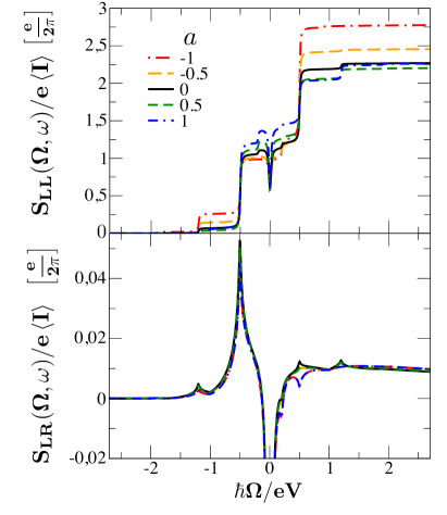
Figure 5: Auto-correlation (top) and cross-correlation noise spectral density (bottom) with ac-driving ($\alpha=1.86$, $\hbar\omega/\gamma=35$, $a=1$). The coincidence of steps in the auto-terminal and peaks in the cross-terminal noise spectra is only partial, since the integrand in dominating contributions probes peaks at different energies. The (local) minimum at $\hbar\Omega=0$ of the (auto) cross-terminal noise translates for the chosen parameters into a Fano factor $F=(+)-0.5$.

in agreement with Fig. 1. For large bias voltages $C^{\mathrm{}}_{L \rightarrow R}(\Omega\rightarrow\infty,V)=0$ whereas $C^{\mathrm{}}_{R \rightarrow L}(\Omega\rightarrow\infty,V)$ and $C^{\mathrm{}}_{L \rightarrow L}(\Omega\rightarrow\infty,V)$ both contribute to the frequency-dependent Fano factor with unity. Thus, for large frequencies the Fano factor approaches $F=2$. Due to the lengthy expressions that occur when finite ac-bias is applied, we provide the analytical results in the appendix, Eqs.(39). Then Fano factors $F>2$ are possible since the average dc-current can be suppressed by the ac-bias voltage. Besides the onsets of the correlators and their interpretation in terms of absorption ($\Omega>0$) and emission ($\Omega<0$) of photons by the scattered quasiparticles there is a second important ingredient that determines the current fluctuations. Namely, if the energy is provided there has to exist a scattering channel so a quasiparticle can contribute to the current and current-noise. This is determined by the integrand, the distance of the resonant level to the chemical potentials of the reservoirs and the resonance width. The interplay of these features will be discussed in the following intensively.

III.1 Effect of finite frequency

In the noise spectrum of Fig. 1 the first step of $S^{\mathrm{}}_{LL}(\Omega)$ is determined by states contributing to $C^{\mathrm{}}_{R\rightarrow L}(\Omega)$. For a centered resonance the distance of the resonance to the chemical potential of the left reservoir is $-eV/2$, so the step is at the corresponding frequency. If we increase the distance to the reservoir of the final state the step is shifted to smaller frequencies so the plateau gets wider. This behavior can be understood by an argument provided by the structure of the involved product of s-matrices (Fig. 2). This product exhibits a single peak at $\epsilon_{r}-\hbar\Omega$ that is only probed by the noise if it is inside the energy window $\mu_{L}-\hbar\Omega\ldots\mu_{R}$ and a small shoulder for energies larger than $\hbar\Omega$. It is clear from above arguments that the step-width is $2\gamma$. Since for frequencies $-eV/2<\hbar\Omega<eV/2$ no further scattering paths exist, the noise stays constant in this regime apart from the dip around $\hbar\Omega=0$. This sub-Poissonian Fano factor can be understood as the effect of electron anti-bunching. Since incoming wave packets hit the scattering region with a rate $1/eV$ and have a temporal extension proportional to $1/\gamma$, a frequency $\hbar\Omega\sim\gamma$ can not probe the correlation between them. This picture is supported by the fact that at frequencies of the order of the resonance width the two correlated events, which are suggested by the Fermi functions, are both in resonance. Namely an electron-like state $f_{R}^{\mathrm{e}}(\epsilon)$ transmitted $T(\epsilon)$ at energy $\epsilon$ from right to left, and a hole state $f_{L}^{\mathrm{h}}(\epsilon+\hbar\Omega)$, reflected at left terminal at energy $\epsilon+\hbar\Omega$ with probability $R(\epsilon+\hbar\Omega)$. So the integrand in $C^{\mathrm{}}_{R\rightarrow L}$ is suppressed by a factor of $2$ (we have a second resonant path) in terms of the interference-like dip around $\epsilon=0$. In the mentioned regime the transmission can still be aligned with the resonance energy leading to the same charge transfer as for higher frequencies, whereas the reflected path is strongly suppressed since $R(\epsilon)\rightarrow 0$ as $\epsilon\rightarrow\epsilon_{r}$, so the ratio $S/eI$ should be suppressed. A similar discussion of the other contributions is straight forward. The main aspects are: The dominating contributions are those where the final state is related to the measurement terminal. This is also the terminal where charge is effectively transferred to. If the energy transferred via PAT events matches the distance of the resonance energy $\epsilon_{r}$ from the chemical potential $\mu_{L}=-eV/2$, then the interference-like term $C^{\mathrm{}}_{L\rightarrow L}$ leads to the second step, located at $\hbar\Omega=eV/2$ in the noise spectrum. Assuming a centered resonance, the integrand for this term exhibits peaks at $\epsilon=0,-\hbar\Omega$. Those peaks unite to a single one when $\hbar\Omega\leq 2\gamma$ (see the black curve in Fig. 2 a) and show destructive interference corresponding to the afore mentioned anti-bunching of the quasiparticles. If $\mu_{L}=\mu_{R}=0$ this behavior is the origin of a small overshoot in the auto-correlation spectrum at frequency $\Omega\leq\gamma$ before the spectrum saturates (not shown in the plots).

If a finite dc-bias is applied, then the peak around $\epsilon=0$ is outside the integration window. But the center of the second peak comes into play when $\hbar\Omega\geq eV/2$, thus we find a step there. The smallest impact on the noise comes from $C^{\mathrm{}}_{R\rightarrow R}(\Omega)$ and $C^{\mathrm{}}_{L\rightarrow R}(\Omega)$ since they probe the tail of the resonance only. The latter one naturally only has a small impact on current-current correlations because a quasiparticle needs to be provided with an energy quantum $\hbar\Omega\geq eV$ in order to overcome the potential difference. Therefore the resonance position, as long as it is inside the bias-window does not affect the onset of the contribution, but modifies the impact on the noise.

III.2 Influence of harmonic ac-driving

Here we have to distinguish between differently coupled light fields, wether the ac-drive is applied at both or one terminal only. The ac-bias voltage opens additional scattering paths as illustrated in Fig. 3 for $C^{\mathrm{}}_{R\rightarrow L}(\Omega,\omega)$ with arbitrary $a$. There, PAT events induced by the ac-bias are considered up to first order. When $a=1$ all contributions to the auto-terminal noise except $C^{\mathrm{}}_{L\rightarrow L}(\Omega,\omega)$ are given by the set of scattering paths determined by the s-matrices without ac-drive. In that case the two Besselfunction corresponding to the not driven terminal generate a Kronecker delta which assures that the two remaining Besselfunctions of the other terminal have the same indices. So the product of all Besselfunctions is positive by definition. Furthermore the arguments of the s-matrices are independent of the driving frequency because only the energies $(m-l)\hbar\omega$ with $m-l=0$ are allowed. Thus, for scattering events where one of the two states is related to a driven reservoir, either the initial or the final one, the ac-driving enters only via the $k\hbar\omega$ or $l\hbar\omega$ terms in the argument of the Fermi functions but leave the integrand unchanged. Consequently, PAT events that are stimulated by the ac-bias voltage show up in all correlators even if initial and final states are not related to the driven terminal. But the number of features that can be identified in the noise spectral function increases when $|a|\neq 1$. Now let us take a closer look on Fig. 4, where $eV=0$ and $\Omega=0$: Starting the analysis with the curve for $a=1$ one can identify the minima and maxima of $S_{LL}(\Omega,\omega)$ with the zeros of the $J_{n}(\alpha)$ when $n=0,1$. The surprising fact that the oscillations have minima when $J_{1}$ vanishes is due to the $n=0$ term which has no contribution to the noise because it does not probe the peak of the involved integrand. But for frequencies larger then $\gamma$ the $n=1$ term does and therefore dominates the charge transport and fluctuations. The same reason leads to the maxima when $J_{0}$ has minima and thereby reduces the weight of the zero-order terms. Because of the completeness of the Besselfunctions then the higher order terms, which are non-zero if $m=l>0$, have a stronger weight and the noise is enhanced. In this example the ac-generated PAT contributions to the noise are related to the left reservoir - the oscillating one - so the correlations $C^{\mathrm{}}_{R\rightarrow R}(\Omega,\omega)$ vanish. The oscillatory behavior of the Besselfunctions is clearly visible for contributions $C_{L\rightarrow L}(\Omega,\omega)$ and for the two cross-contributions to $S_{LL}^{\mathrm{}}(\Omega=0,\omega)$. These are identical and exhibit even more pronounced oscillations, with a maximal contribution of $C_{\alpha\rightarrow\beta}(\Omega,\omega)/eI=0.125$.

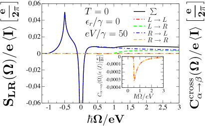
Figure 6: Frequency dependence of the zero-temperature current-current cross-correlations for $\epsilon_{r}=0$. The minima at $\hbar\Omega\rightarrow 0$ is given by $\left.S_{LR}=-S_{LL}\right|_{\Omega=0}$. Dominating terms inside the integration intervals are originating from the cross-terminal contribution. The inset shows a zoom into auto-terminal terms, which are identical ($\epsilon_{r}=0$) and orders of magnitude smaller than cross-terminal ones due to the sharp resonance considered. Now a peak-like structure can be observed instead of the step-like behavior observed in the auto-correlation spectrum.

That’s why the two limiting cases $a=1$ and $a=0$ have maximal values of $0.5$ and $0.375$. If the asymmetry in the driving is reduced, as done above (meaning we increase the amplitude of the driving with opposite sign at the second reservoir), the contributions $C^{\mathrm{}}_{R\rightarrow R}(\Omega,\omega)$ are finite. As an example we analyse the curve for $a=0.5$. This means in the left reservoir we have an effective driving of the order $0.75\alpha$ while at the right reservoir of the order $0.25\alpha$. Consequently for $C^{\mathrm{}}_{L\rightarrow L}(\Omega,\omega)$ we find maxima where $J_{n}(0.75\alpha)$ has minima and for $C^{\mathrm{}}_{R\rightarrow R}(\Omega,\omega)$ where $J_{n}(0.25\alpha)$ has minima. Since we are analyzing a situation where $\epsilon_{r}=0$ (symmetric setup) the two cross-contributions $C^{\mathrm{}}_{\alpha\rightarrow\beta}(\Omega,\omega)$ ($\alpha\neq\beta$) to the auto-correlation noise are identical at $eV=0$, showing minima at intermediate positions between the expected minima related to $\alpha_{L}$ and $\alpha_{R}$. Concerning the cross-correlation spectrum at $\hbar\Omega=0$ as a function of the driving the results are analogues. The curve starts at $S_{LR}(\alpha=0)=0$ and oscillates around negative values between $-1/2\ldots-3/8$ ($a=-1\ldots 1$). At finite voltage the curves start at $\pm 1/2$ and still show the oscillations due to the Besselfunctions. But, e.g. for the auto-correlator in our setup, contributions scattered into the left reservoir (the driven one) are again dominant. Then the $C_{R\rightarrow L}(\Omega,\omega)$ term is the one giving the finite value at zero driving, consistent with the dc noise spectra. The second dominant contribution at $\hbar\Omega=0$, $C_{L\rightarrow L}(\Omega,\omega)$, is switched on by the driving voltage. When an additional ac-bias voltage is applied, the noise spectral function as plotted in Fig. 5 acquires additional steps due to PAT events related to the driving. The height of the steps is non-universal and determined by the Besselfunctions. Since the arguments $\alpha_{L/R}$ stay constant, the step-height height decreases for large $n$ and oscillates as a function of $\alpha$. It vanishes at nodes of the Besselfunctions, analogues to the limit of energy-independent scattering as studied for ac-biased junctions in Ref. LesovikLevitov94 . For vanishing ac-drive only the zero order Besselfunction should contribute, thus we find a step height proportional to $J_{0}(0)=1$. Besides the dip around $\hbar\Omega=0$ one now expects further features in the noise at frequencies $\hbar\Omega=\mu_{\alpha}-\epsilon_{r}\pm n\hbar\omega$ with $\alpha=L,R$.

IV Current-current cross-correlations

In this section we focus on the cross-correlation noise spectral function. Again we write contributions to the zero temperature noise explicitly as a sum.

$$S_{LR}(\Omega,\omega)=\underset{\alpha,\beta=L,R}{\sum}C^{\mathrm{cross}}_{\alpha\rightarrow\beta}(\Omega,\omega)$$ (19)

determines the cross-correlation noise spectrum where the $C^{\mathrm{cross}}_{\alpha\rightarrow\beta}(\Omega)$ are in general complex quantities. If $\alpha=\beta$ the correlators $C^{\mathrm{cross}}_{\alpha\rightarrow\alpha}(\Omega)\in\mathcal{R}$ at $\hbar\Omega=0$ in the dc-limit. Accordingly, at finite frequency these terms acquire a phase factor. The different contributions in the dc-limit read

$$C^{\mathrm{cross}}_{L\rightarrow L}(\Omega)= \frac{e^{2}\Theta(\hbar\Omega)}{2\pi\hbar}\underset{\mu_{L}-\hbar\Omega}{\overset{\mu_{L}}{\int}}d\epsilon\,$$

$$t^{*}(\epsilon+\hbar\Omega)t(\epsilon)\left[r^{*}(\epsilon)r(\epsilon+\hbar\Omega)-1\right]$$ (20a)

$$C^{\mathrm{cross}}_{R\rightarrow R}(\Omega)= \frac{e^{2}\Theta(\hbar\Omega)}{2\pi\hbar}\underset{\mu_{R}-\hbar\Omega}{\overset{\mu_{R}}{\int}}d\epsilon\,$$

$$t^{*}(\epsilon)t(\epsilon+\hbar\Omega)\left[r^{*}(\epsilon+\hbar\Omega)r(\epsilon)-1\right]$$ (20b)

$$C^{\mathrm{cross}}_{L\rightarrow R}(\Omega)= \frac{e^{2}\Theta(\hbar\Omega-eV)}{2\pi\hbar}\underset{\mu_{R}-\hbar\Omega}{\overset{\mu_{L}}{\int}}d\epsilon\,$$

$$r^{*}(\epsilon)t(\epsilon)r^{*}(\epsilon+\hbar\Omega)t(\epsilon+\hbar\Omega)$$ (20c)

$$C^{\mathrm{cross}}_{R\rightarrow L}(\Omega)= \frac{e^{2}\Theta(\hbar\Omega+eV)}{2\pi\hbar}\underset{\mu_{L}-\hbar\Omega}{\overset{\mu_{R}}{\int}}d\epsilon\,$$

$$t^{*}(\epsilon)r(\epsilon)t^{*}(\epsilon+\hbar\Omega)r(\epsilon+\hbar\Omega)$$ (20d)

The onsets of the $C^{\mathrm{cross}}_{\alpha\rightarrow\beta}(\Omega)$ are the same as before. As shown in Fig. 6, the finite frequency cross-correlation noise spectrum can be positive as it is also the case in superconducting systems Martin08 ; Buzdin09 . Steps in the auto-correlation spectrum now translate into peaks at negative and into dips at positive frequencies as it can be seen in Fig. 6. To shine a light on the this difference it is again fruitful to study the shape of the integrands involved. In comparison to auto-correlations, cross-correlations exhibit a different symmetry in the pairing of s-matrices. The cross-contributions to $S_{\alpha\beta}(\Omega,\omega)$ are similar to the auto-correlation contributions to $S_{\alpha\alpha}(\Omega,\omega)$ and vice versa. In detail, the main contribution now originates from $C^{\mathrm{cross}}_{R\rightarrow L}$. Similar to the integrand shown in Fig. 2 for auto-correlation noise with ac-driving, the integrand and thus the correlator itself can be negative. At frequencies $\hbar\Omega\leq\gamma$ the correlations between opposite terminals are negative by definition, due to the unitarity of the s-matrix. In this regime the integrand takes negative values whereas for energies $\hbar\Omega\gg\gamma$ a positive contribution emerges due to PAT. An off-centered resonance splits the peak at $\hbar\Omega=-eV/2$ in $C^{\mathrm{cross}}_{R\rightarrow L}$ symmetrically, in analogy to the shifting of the step position in the current-current auto-correlation spectrum, Fig 1. If $\epsilon_{r}>|eV/2|$ these two peaks at $\hbar\Omega=-eV/2\pm\epsilon_{r}$ move towards $\Omega=-eV,0$ where they vanish and the noise spectrum gets negative along the whole emission branch ($\Omega<0$). As for the auto-correlation noise spectrum, at $k_{B}\mathcal{T}=0$ the cross-correlation noise spectrum can be calculated analytically by assuming a Breit-Wigner lineshape, Eq. (4). Integration of Eqs.(20) yields

$$C^{\mathrm{cross}}_{L\rightarrow L}(\Omega)= \Theta(\Omega)f(\Omega)(1+i\Omega/\gamma)F(\mu_{L}-\epsilon_{r},\Omega)$$ (21a)

$$C^{\mathrm{cross}}_{R\rightarrow R}(\Omega)= \Theta(\Omega)f(\Omega)(1-i\Omega/\gamma)F(\mu_{R}-\epsilon_{r},\Omega)$$ (21b)

$$C^{\mathrm{cross}}_{L\rightarrow R}(\Omega)= -\Theta(\Omega-eV)f(\Omega)\left.K(\epsilon-\epsilon_{r},\Omega)\right|^{\mu_{L}}_{\mu_{R}-\Omega}$$ (21c)

$$C^{\mathrm{cross}}_{R\rightarrow L}(\Omega)= -\Theta(\Omega+eV)f(\Omega)\left.K(\epsilon-\epsilon_{r},\Omega)\right|^{\mu_{R}}_{\mu_{L}-\Omega}\,,$$ (21d)

where the functions $F(\epsilon,\Omega)$ and $K(\epsilon,\Omega)$ are defined in the appendix, see Eqs. (27)-(38). As for the auto-terminal noise, the correlator $C^{\mathrm{cross}}_{R\rightarrow L}(\Omega)$ is equal to $C^{\mathrm{cross}}_{L\rightarrow R}(\Omega)$ when the reservoir indices $L,R$ are interchanged, and thus the voltage in the Heaviside theta function changes sign, too. $C^{\mathrm{cross}}_{R\rightarrow R}(\Omega)$ is equal to $C^{\mathrm{cross}}_{L\rightarrow L}(\Omega)$ if we take the complex conjugate of the pre-factor $(1+i\Omega/\gamma)$. Overall the solutions are very similar to the auto-terminal noise spectral function were the most prominent difference is the imaginary part occurring in the pre-factors. Again the results can be simplified for a symmetric setup, leading to the replacements $\left.K(\epsilon-\epsilon_{r},\Omega)\right|^{\mu_{R}}_{\mu_{L}-\Omega}\rightarrow-2K(V/2,\Omega)$ and $\left.K(\epsilon-\epsilon_{r},\Omega)\right|^{\mu_{L}}_{\mu_{R}-\Omega}\rightarrow 2K(V/2,-\Omega)$. At $\Omega=0$ the noise power is given by $S_{LR}(0)=C^{\mathrm{cross}}_{R\rightarrow L}(0)$ with

$$C^{\mathrm{cross}}_{R\rightarrow L}(0)=\frac{-e^{2}\gamma\Theta(eV)}{4\hbar}\left(\frac{\gamma(\mu_{L}-\epsilon_{r})}{\gamma^{2}+(\mu_{L}-\epsilon_{r})^{2}}\right.$$

$$\left.-\frac{\gamma(\mu_{R}-\epsilon_{r})}{\gamma^{2}+(\mu_{R}-\epsilon_{r})^{2}}+\text{atan}\left[\frac{\mu_{R}-\epsilon_{r}}{\gamma}\right]-\text{atan}\left[\frac{\mu_{L}-\epsilon_{r}}{\gamma}\right]\right)\,$$ (22)

Assuming $\gamma\ll\mu_{L/R}-\epsilon_{r}$ this results in $C^{\mathrm{cross}}_{R\rightarrow L}(0)=-\frac{e^{2}\gamma\pi}{2\hbar}$ and thus a Fano factor $F=-1/2$. At $\Omega=0$ the sum of all correlations vanishes $S_{LR}(0)+S_{LL}(0)+S_{RL}(0)+S_{RR}(0)=0$ since in this limit all s-matrices are probed at the same energy. In the limit $|\hbar\Omega|\gg|eV|$ all correlators that contribute to the cross-correlation noise spectrum vanish.

Now we switch on the ac-bias voltage and set $\Omega,\epsilon_{r}=0$. Then the auto-terminal contributions to the cross-correlation spectrum are real and can therefore be described by the product of two transmission probabilities. Cross-terminal contributions are related by complex conjugation. In this limit we can use the transmission functions introduced in Eq. (14) to express the integrands defined by Eq. (5) in an intuitive way as

$$M^{\mathrm{cross}}_{L\rightarrow L}(\omega_{m-l},0) =M^{\mathrm{cross}}_{R\rightarrow R}(\omega_{m-l},0)$$

$$=T(\epsilon)T(\epsilon+(m-l)\hbar\omega)$$ (23a)

$$M^{\mathrm{cross}}_{L\rightarrow R}(\omega_{m-l},0) =\left[M^{\mathrm{cross}}_{R\rightarrow L}(\omega_{m-l},0)\right]^{*}$$

$$=T(0,\epsilon+(m-l)\hbar\omega)R(0,\omega_{m-l})\,.$$ (23b)

We give our analytical results for the cross-correlation noise spectral function when a finite ac-bias is applied in the appendix, Eqs. (40). Corresponding noise spectra are presented in Fig. 5 for different values of $a$.

V Energy independent scattering and elementary charge transfer processes

In the scattering approach without interaction it is straightforward to go from the single level setup that we have concentrated on, to two or more energy levels. If there is no internal coupling of the levels, the current as well as the current noise through the involved resonances is just the sum of the independent contributions. Cross-over from an energy-independent scattering to the multi-level case turns the straight lines shape of the noise power discussed before into a sequence of steps at the resonance energies. If the energy levels are internally coupled the difficulty is to find the corresponding s-matrix. For two coupled levels at zero bias voltage the frequency-dependence of shot noise has been studied recently EntinWohlman07 . Although the resonant levels fingerprint in the spectra gives a lot of benefits when interpreting the data and identifying scattering channels, its energy dependence also brings a bunch of complications. Especially the events can not be defined by transmission and reflection probabilities, which connect occupied and unoccupied states in the reservoirs. If one drops this energy dependence, Imry et. al. GavishImry01 have shown that the four contributions to the noise are proportional to the Bose-distribution function $n_{B}(\epsilon)$. Interestingly this originates from the product $f_{\alpha}(\epsilon)\left(1-f_{\beta}(\epsilon+\hbar\Omega)\right)$, which can also be written as $\left(n_{B}(\Omega)+1\right)\left(f_{\alpha}(\epsilon)-f_{\beta}(\epsilon+\hbar\Omega)\right)$. Integration over all energies yields $\hbar\Omega\left(n_{B}(\Omega)+1\right)$, what is again proportional to the photon distribution. In this way the four contributions are proportional to $M_{\beta\rightarrow\alpha}x_{\alpha\beta}(n_{B}(_{\alpha,\beta})+1)$, with $x_{LL}=x_{RR}=\hbar\Omega$, $x_{LR}=\hbar\Omega-eV$ and $x_{RL}=\hbar\Omega+eV$.

In Refs. VanevicBelzig07 ; VanevicBelzig08 the noise power has been studied for systems with time-dependent voltages as an interplay between unidirectional and bidirectional events of charge transfer. Those events can be related to the four correlators of the shot-noise spectrum, even at energy-dependent scattering (see also Fig 3). Let us first set $\alpha,\hbar\Omega,k_{B}\mathcal{T}=0$. Then current-fluctuations are determined by $C_{R\rightarrow L}(\Omega,\omega)$ and are a pure source of unidirectional events. If there is a free state in reservoir $L$ an electron in $R$ is either reflected back to reservoir $R$ or transmitted to $L$. Thus, the whole process is proportional to $T(\epsilon)R(\epsilon)f^{\mathrm{e}}_{R}(\epsilon)f^{\mathrm{h}}_{R}(\epsilon)$. For symmetric bias $\mu_{L}=-\mu_{R}<0$ the analogues hole-like process is equivalent and describes effective electron transfer from $R$ to $L$ with same probability. At finite $\Omega$ the correlator $C_{R\rightarrow L}(\Omega,0)$ is proportional to $T(\epsilon)R(\epsilon)f^{\mathrm{e}}_{R}(\epsilon)f^{\mathrm{h}}_{L}(\epsilon+\hbar\Omega)$. Or in terms of electron-like events this can be written with the help of the photonic-distribution $n_{B}(\epsilon)=1/[\mathrm{Exp}[\epsilon/k_{B}\mathcal{T}]-1]$ as $T(\epsilon)R(\epsilon)(n_{B}(\Omega)+1)(f^{\mathrm{e}}_{R}(\epsilon)-f^{\mathrm{e}}_{L}(\epsilon+\hbar\Omega))$. Thus, we probe photonic fluctuations due to a virtual electron-hole pair created by the frequency in lead $L$, with one partner being transmitted and the other one being reflected. $C_{L\rightarrow R}(\Omega,0)$ describes the equivalent process with electron-hole pair generation in terminal $R$ with effective charge transfer to the right. $C_{L\rightarrow L}(\Omega,0)$ couples electron and hole paths during reflection in the scattering region via $r^{*}(\epsilon)r(\epsilon+\hbar\Omega)$, what also introduces a finite scattering phase as discussed in section II. $C_{R\rightarrow R}(\Omega,0)$ then probes the difference in the transmission of electron-hole excitations incident from the right, described by $f^{\mathrm{e}}_{R}(\epsilon)-f^{\mathrm{e}}_{R}(\epsilon+\hbar\Omega)$. Although auto-terminal correlators depend on a single chemical potential, rather than the bias voltage, the interplay with PAT processes gives rise to photo-assisted unidirectional events of charge transfer. Now we finally examine the case of finite ac-bias $eV_{\mathrm{ac},L}\cos(\omega t)$ at $\hbar\Omega,k_{B}\mathcal{T}=0$. Then both cross-contributions still describe unidirectional ($l=0$) and bidirectional events ($l\neq 0$) via

$$S {}^{\mathrm{uni+bi}}_{LL}(\omega)=\frac{e^{2}}{2\pi\hbar}\underset{l}{\sum}J^{2}_{l}(\alpha_{L})\int\limits_{-\infty}^{\infty}T(\epsilon)(1-T(\epsilon))d\epsilon$$

$$\left(f^{\mathrm{e}}_{R}(\epsilon)f^{\mathrm{h}}_{L}(\epsilon-l\hbar\omega)+f^{\mathrm{e}}_{L}(\epsilon-l\hbar\omega)f^{h}_{R}(\epsilon)\right)\,.$$ (24)

E.g. the first term refers to events that are proportional to $T(\epsilon)T(\epsilon_{m-l})(n_{B}(l\hbar\omega)+1)(f^{\mathrm{e}}_{R}(\epsilon)-f^{\mathrm{e}}_{L}(\epsilon-l\hbar\omega))$, with electron-hole pair creation in the driven ($L$) terminal for $l\neq 0$. Auto-terminal contributions are given by

$$S^{\mathrm{ac}}_{LL}(\omega) =\frac{e^{2}}{2\pi\hbar}\underset{\beta;k,l,m}{\sum}J_{l}\left(\alpha_{\beta}\right)J_{k}\left(\alpha_{\beta}\right)J_{m}\left(\alpha_{\beta}\right)J_{l+k-m}\left(\alpha_{\beta}\right)$$

$$\int\limits_{-\infty}^{\infty}d\epsilon\,T(\epsilon)T(\epsilon_{m-l})f^{e}_{\beta}(\epsilon_{-l})f^{h}_{\beta}(\epsilon_{-k})\,,$$ (25)

where $\beta=L,R$ and $\epsilon_{n}\equiv\epsilon+n\hbar\omega$. Since we set $\alpha_{R}=0$, the term with $\beta=R$ vanishes at $k_{B}\mathcal{T}=0$. This purely ac-induced contribution can not be interpreted by bidirectional events. If $\beta=L$, virtual electron-hole pairs are generated in the left reservoir. Thus, the two particles are incident from the left, but now both species are transmitted with different probabilities where the whole process is proportional to $T(\epsilon)T(\epsilon_{m-l})$. Therefor, the correlator describes events where both particles move into the same direction. In this way both auto-terminal contributions refer to ac-induced unidirectional charge transfer events scattered towards the measurement terminal. If the resonance is very narrow ($\gamma\ll eV,\hbar\omega$), the product $T(\epsilon)T(\epsilon_{m-l})$ will be very small if $m\neq l$. Then the main contributions from Eq.(25) are expected when $l=m$. By assuming energy-independent scattering, the correlators can be expressed in terms of the photonic distribution as

$$C^{\mathrm{}}_{L\rightarrow L} =\frac{e^{2}}{2\pi\hbar}T^{2}\underset{k,l,m}{\sum}J_{l}\left(\alpha_{L}\right)J_{k}\left(\alpha_{L}\right)J_{m}\left(\alpha_{L}\right)J_{l+k-m}\left(\alpha_{L}\right)$$

$$\times\left[n_{B}((l-k)\hbar\omega)+1\right](l-k)\hbar\omega$$ (26a)

$$C^{\mathrm{}}_{L\rightarrow R} =\frac{e^{2}}{2\pi\hbar}T(1-T)\underset{l}{\sum}J_{l}^{2}\left(\alpha_{L}\right)(l\hbar\omega-eV)$$

$$\times\left[n_{B}(l\hbar\omega-eV)+1\right]$$ (26b)

$$C^{\mathrm{}}_{R\rightarrow L} =\frac{e^{2}}{2\pi\hbar}T(1-T)\underset{l}{\sum}J_{l}^{2}\left(\alpha_{L}\right)(eV-l\hbar\omega)$$

$$\times\left[n_{B}(eV-l\hbar\omega)+1\right]$$ (26c)

$$C^{\mathrm{}}_{R\rightarrow R} =\frac{e^{2}k_{B}\mathcal{T}}{2\pi\hbar}T^{2}\,,$$ (26d)

where we have assumed $a=1$ and identical temperatures $\mathcal{T}$ in both reservoirs. We have also dropped the arguments on the left hand side for compacter notation. On one hand, dc-induced unidirectional events are determined by the the cross-terminal contributions. On the other hand, bidirectional events are due to photonic fluctuations and the associated electron-hole pairs induced in the driven terminal. This terminal ($L$) affects three out of the four correlators. If both distribution functions refer to the ac-biased terminal, as in $C^{\mathrm{}}_{L\rightarrow L}(\omega)$, we have ac-induced unidirectional events.

VI Conclusions

In summary we have interpreted the asymmetric noise spectra of an coherent-scattering double-barrier system with a single resonant level. We calculated an analytical solution for the photo-assisted noise spectral function for auto-terminal and cross-terminal current-current correlations at $k_{B}\mathcal{T}=0$ by assuming a Breit-Wigner lineshape for the resonance. At finite frequency or finite ac-bias shot noise is produced by partitioning of electron-hole pairs. As a consequence, this simple system shows a noise spectrum sensitive to many parameters. It exhibit signatures of quantum-coherent current-current correlations as a sub-Poissonian Fano factor around the resonance energy. This anti-bunching of electrons is in competition with the PAT events, stimulated by the ac-driving ($n\hbar\omega$) or a static electric field $(\hbar\Omega)$. At frequencies $\hbar\Omega\geq\epsilon_{r}+eV/2$ we find a super-Poissonian Fano factor for the auto-terminal noise and positive values for the cross-terminal noise when $\hbar\Omega\gg\gamma$. Furthermore we have shown how the scattering events can be assigned to the four different combinations of final and initial electronic states. Cross-terminal contributions to the auto-correlation noise spectral function can be related to the unidirectional and bidirectional elementary events of charge transfer identified in a recent microscopic derivationVanevicBelzig07 . But the scattering approach also reveals an additional kind of processes where the ac-bias voltage induces unidirectional events directed towards the measurement terminal. In the limit $\hbar\Omega\rightarrow 0$ we could express the photo-assisted noise in terms of the photonic distribution function. The scattering formalism gives insight to the connection between the different regimes discussed throughout this article. Moreover, it also allows us to connect the interpretation of shot noise obtained via different approaches, e.g. by FCS or a discussion in terms of wave packets via the Fermi golden rule. The steps and dips of the noise spectra can be used in experiments to extract information about the resonance position, effective chemical potentials or in general to get insight into the coupling of the laser-field to the system in terms of PAT.

VII Acknowledgement

We would like to acknowledge financial support by the DFG through SFB 767 and SP 1285.

VIII Appendix: Analytic solution

By the help of the definitions below we can write the analytic solutions for the non-symmetrized noise spectrum in a compact way. If only dc-bias voltages are present, it turns out to be convenient to introduce the pre-factor

$$f(\Omega)= \frac{e^{2}\gamma^{3}}{2\left(4\gamma^{2}+\Omega^{2}\right)}\,.$$ (27)

Furthermore we use the expressions

$$F(\epsilon,\Omega) =\text{atan}\left(\frac{\epsilon+\Omega}{\gamma}\right)-\text{atan}\left(\frac{\epsilon-\Omega}{\gamma}\right)$$

$$- \frac{\gamma}{\Omega}\ln\left[\frac{(\gamma^{2}+\epsilon^{2})^{2}}{\left(\gamma^{2}+\left(\epsilon+\Omega\right)^{2}\right)\left(\gamma^{2}+\left(\epsilon-\Omega\right)^{2}\right)}\right]$$ (28)

$$G(\epsilon,\Omega) =\left[3+\left(\frac{\Omega}{\gamma}\right)^{2}\right]\text{atan}\left(\frac{\epsilon+\Omega}{\gamma}\right)-\text{atan}\left(\frac{\epsilon}{\gamma}\right)$$

$$+ \frac{\gamma}{\Omega}\ln\left[\frac{\gamma^{2}+\epsilon^{2}}{\gamma^{2}+\left(\epsilon+\Omega\right)^{2}}\right]$$ (29)

$$H(\epsilon,\Omega) =\left[2+\left(\frac{\Omega}{\gamma}\right)^{2}\right]\left(\text{atan}\left(\frac{\epsilon+\Omega}{\gamma}\right)+\text{atan}\left(\frac{\epsilon}{\gamma}\right)\right)$$

$$+ 2\frac{\gamma}{\Omega}\ln\left[\frac{\gamma^{2}+\epsilon^{2}}{\gamma^{2}+\left(\epsilon+\Omega\right)^{2}}\right]$$ (30)

for auto- and cross-terminal noise. To achieve a compact notation for the cross-terminal noise we also need the definition

$$K(\epsilon,\Omega) =\text{atan}\left(\frac{\epsilon+\Omega}{\gamma}\right)+\text{atan}\left(\frac{\epsilon}{\gamma}\right)$$

$$+ \frac{\gamma^{2}+\Omega^{2}/2}{\gamma\Omega}\ln\left[\frac{\gamma^{2}+\epsilon^{2}}{\gamma^{2}+\left(\epsilon+\Omega\right)^{2}}\right]\,.$$ (31)

If additional ac-bias voltages are present it is reasonable to make use of the pre-factor

$$\tilde{f}(\Omega)=\frac{e^{2}\gamma^{4}}{4}$$ (32)

and the shorthands

$$D_{1}= \left[(2i\gamma+\Omega)(2i\gamma+\omega)(\Omega+\omega)\right]^{-1}$$ (33)

$$D_{2}= \left[(2i\gamma+\Omega)(-2i\gamma+\omega)(\Omega-\omega)\right]^{-1}$$ (34)

$$D^{\pm}_{3}= 2\gamma(i\gamma\pm\Omega+\omega)$$ (35)

$$D^{\pm}_{4}= 2(\gamma\pm i\Omega)(i\gamma+\omega)\,.$$ (36)

Finally we complete the set of functions with

$$A^{\pm}(\epsilon,\Omega,\omega) =2i\text{atan}\left(\frac{\epsilon+\Omega+\omega}{\gamma}\right)$$

$$\pm \ln\left(\gamma^{2}+(\epsilon+\Omega+\omega)^{2}\right)$$ (37)

$$B^{\pm}(\Omega,\omega) =2(\gamma+i\Omega)(\pm i\gamma+\Omega+\omega)\,,$$ (38)

where $A^{\pm}(\epsilon,\Omega,\omega)$ defines the basic shape of the results for ac-biased systems and $B^{\pm}(\Omega,\omega)$ is needed for the description of the cross-correlation spectrum. Below we present the results for the photo-assisted noise spectral density of auto-terminal and cross-terminal current-current correlations. We assume a Breit-Wigner lineshape (4) for the resonant level and perform the energy integration in Eqn.(5). The results are plotted as a function of frequency in Fig.5. Due to the cumbersome expressions we use the shorthands defined above as well as the notation $\tilde{\omega}\equiv(m-l)\hbar\omega$ and set $\hbar=1$. For the auto-correlation function we then find

$$C^{\mathrm{}} {}_{L \rightarrow L}(\Omega,\omega)=\tilde{f}(\Omega)(1+(\Omega/\gamma)^{2})\sum\limits_{lkm}\Theta(\Omega+(l-k)\omega)J_{l}\left(\alpha_{L}\right)J_{k}\left(\alpha_{L}\right)J_{m+k-l}\left(\alpha_{L}\right)J_{m}\left(\alpha_{L}\right)\big{[}\big{.}$$

$$\big{.}-D_{1}A^{-}(\epsilon,0,0)+D_{2}A^{-}(\epsilon,\Omega,0)-D_{2}^{*}A^{-}(\epsilon,\Omega,\tilde{\omega})+D_{1}^{*}A^{-}(\epsilon,0,\tilde{\omega})\big{]}^{\epsilon=\mu_{L}+l\omega}_{\epsilon=\mu_{R}-\Omega+k\omega}$$ (39a)

$$C^{\mathrm{}} {}_{R \rightarrow R}(\Omega,\omega)=\tilde{f}(\Omega)\sum\limits_{lkm}\Theta(\Omega+(l-k)\omega)J_{l}\left(\alpha_{L}\right)J_{k}\left(\alpha_{L}\right)J_{m+k-l}\left(\alpha_{L}\right)J_{m}\left(\alpha_{L}\right)\big{[}\big{.}$$

$$\big{.}D_{1}A^{+}(\epsilon,0,0)+D_{1}^{*}A^{-}(\epsilon,0,\tilde{\omega})-D_{2}^{*}A^{-}(\epsilon,\Omega,0)-D_{2}^{*}A^{+}(\epsilon,\Omega,\tilde{\omega})\big{]}^{\epsilon=\mu_{R}+l\omega}_{\epsilon=\mu_{R}-\Omega+k\omega}$$ (39b)

$$C^{\mathrm{}} {}_{L \rightarrow R}(\Omega,\omega)=\tilde{f}(\Omega)\sum\limits_{lkm}\Theta(\Omega+(l-k)\omega-eV)J_{l}\left(\alpha_{L}\right)J_{k}\left(\alpha_{R}\right)J_{m+k-l}\left(\alpha_{R}\right)J_{m}\left(\alpha_{L}\right)\big{[}\big{.}$$

$$\big{.}B^{+}(0,\tilde{\omega})D_{1}A^{+}(\epsilon,0,0)+B^{-}(\Omega,\tilde{\omega})D_{1}^{*}A^{+}(\epsilon,\Omega,\tilde{\omega})+B^{-}(-\Omega,\tilde{\omega})D_{2}A^{+}(\epsilon,\Omega,0)+B^{+}(0,\tilde{\omega})D_{2}^{*}A^{-}(\epsilon,0,\Omega)\big{]}^{\epsilon=\mu_{L}+l\omega}_{\epsilon=\mu_{R}-\Omega+k\omega}$$ (39c)

$$C^{\mathrm{}} {}_{R \rightarrow L}(\Omega,\omega)=\tilde{f}(\Omega)\sum\limits_{lkm}\Theta(\Omega+(l-k)\omega+eV)J_{l}\left(\alpha_{R}\right)J_{k}\left(\alpha_{L}\right)J_{m+k-l}\left(\alpha_{L}\right)J_{m}\left(\alpha_{R}\right)\big{[}B^{+}(0,\tilde{\omega})D_{1}A^{-}(\epsilon,0,0)+\big{.}$$

$$\big{.}+B^{-}(-\Omega,\tilde{\omega})D_{2}A^{-}(\epsilon,\Omega,0)+B^{+}(0,\tilde{\omega})D_{2}^{*}A^{+}(\epsilon,0,\Omega)+B^{-}(\Omega,\tilde{\omega})D_{1}^{*}A^{+}(\epsilon,\Omega,\tilde{\omega})\big{]}^{\epsilon=\mu_{L}+l\omega}_{\epsilon=\mu_{L}-\Omega+k\omega}\,.$$ (39d)

Using the same notation the solution of the cross-terminal correlations can be cast in the form

$$C^{\mathrm{cross}}_{L \rightarrow L}(\Omega,\omega) =\sum\limits_{lkm}\Theta(\Omega+(l-k)\omega)J_{l}\left(\alpha_{L}\right)J_{k}\left(\alpha_{L}\right)J_{m+k-l}\left(\alpha_{L}\right)J_{m}\left(\alpha_{L}\right)\big{[}\big{.}$$

$$\big{.}D_{1}A^{+}(\epsilon,0,0)-D_{1}^{*}A^{+}(\epsilon,\Omega,\tilde{\omega})-D_{2}A^{+}(\epsilon,\Omega,0)+D_{2}^{*}A^{-}(\epsilon,0,\tilde{\omega})\big{]}^{\epsilon=\mu_{L}+l\omega}_{\epsilon=\mu_{L}-\Omega+k\omega}$$ (40a)

$$C^{\mathrm{cross}}_{R \rightarrow R}(\Omega,\omega) =\sum\limits_{lkm}\Theta(\Omega+(l-k)\omega)J_{l}\left(\alpha_{R}\right)J_{k}\left(\alpha_{R}\right)J_{m+k-l}\left(\alpha_{R}\right)J_{m}\left(\alpha_{R}\right)\big{[}\big{.}$$

$$\big{.}D_{1}A^{+}(\epsilon,0,0)-D_{1}^{*}A^{-}(\epsilon,\Omega,\tilde{\omega})-D_{2}A^{-}(\epsilon,\Omega,0)+D_{2}^{*}A^{+}(\epsilon,0,\tilde{\omega})\big{]}^{\epsilon=\mu_{R}+l\omega}_{\epsilon=\mu_{R}-\Omega+k\omega}$$ (40b)

$$C^{\mathrm{cross}}_{L \rightarrow R}(\Omega,\omega) =\sum\limits_{lkm}\Theta(\Omega+(l-k)\omega-eV)J_{l}\left(\alpha_{L}\right)J_{k}\left(\alpha_{R}\right)J_{m+k-l}\left(\alpha_{R}\right)J_{m}\left(\alpha_{L}\right)\big{[}\big{.}$$

$$\big{.}D^{+}_{3}D_{1}A^{+}(\epsilon,0,0)+(D_{3}^{+})^{*}D_{1}^{*}A^{-}(\epsilon,\Omega,\tilde{\omega})+(D_{4}^{+})^{*}D_{2}A^{+}(\epsilon,\Omega,0)+D_{4}^{+}D_{2}^{*}A^{-}(\epsilon,0,\tilde{\omega})\big{]}^{\epsilon=\mu_{L}+l\omega}_{\epsilon=\mu_{R}-\Omega+k\omega}$$ (40c)

$$C^{\mathrm{cross}}_{R \rightarrow L}(\Omega,\omega) =\sum\limits_{lkm}\Theta(\Omega+(l-k)\omega+eV)J_{l}\left(\alpha_{R}\right)J_{k}\left(\alpha_{L}\right)J_{m+k-l}\left(\alpha_{L}\right)J_{m}\left(\alpha_{R}\right)\big{[}\big{.}$$

$$\big{.}D^{-}_{4}D_{1}A^{-}(\epsilon,0,0)+(D_{4}^{-})^{*}D_{1}^{*}A^{+}(\epsilon,\Omega,\tilde{\omega})+(D_{3}^{-})^{*}D_{2}A^{-}(\epsilon,\Omega,0)+D_{3}^{-}D_{2}^{*}A^{+}(\epsilon,0,\tilde{\omega})\big{]}^{\epsilon=\mu_{R}+l\omega}_{\epsilon=\mu_{L}-\Omega+k\omega}\,,$$ (40d)

In the dc-limit these expressions simplify to Eqs. (16) for auto-correlation noise and Eqs. (21) for cross-correlation noise. Obviously, the additional ac-bias introduces a complicated scattering phase via the imaginary parts in the above expressions. The noise spectrum is plotted for different asymmetry parameters $a$ in Fig. 5. Ac-bias voltages introduce additional peaks and dips related to the driving frequency $\omega$. By varying $a$, such PAT induced peaks in the cross-correlation noise spectra can turn into dips and vice versa.

References

References

- (1) L.S. Levitov and G.B. Lesovik, JETP Lett. 58, 230 (1993)
- (2) Ya. Blanter and M. Büttiker, Physics Reports 336, 1 (2000)
- (3) C. Schönenberger, and C. Beenakker, Physics Today 56, 37 (2003)
- (4) Quantum Noise in Mesoscopic Physics, edited by Y.V. Nazarov (Kluwer, Dordrecht, 2003).
- (5) D.A. Wharam et al., J. Phys. C 21, L209 (1988)
- (6) B.J. van Wees et. al., Phys. Rev. Lett. 60, 848 (1988)
- (7) M. Büttiker, H. Thomas, A. Prêtre, Z. Phys. B 94, 133 (1994)
- (8) L.S. Levitov, H. Lee, and G.B. Lesovik, J. Math. Phys. 37, 4845 (1996)
- (9) W. Belzig and Yu. V. Nazarov, Phys. Rev. Lett. 87, 197006 (2001).
- (10) W. Belzig and Yu. V. Nazarov, Phys. Rev. Lett. 87, 067006 (2001).
- (11) Yu.V. Nazarov and D.A. Bagrets, Phys. Rev. Lett. 88, 196801 (2002)
- (12) W. Belzig, Phys. Rev. B 71, 161301 (2005)
- (13) C. Emary, D. Marcos, R. Aguado, and T. Brandes, Phys. Rev. B 76, 161404 (2007)
- (14) M. Vanevic, Y.V. Nazarov, and W. Belzig, Phys. Rev. Lett. 99, 076601 (2007)
- (15) M. Vanevic, Y.V. Nazarov, and W. Belzig, Phys. Rev. B 78, 245308 (2008)
- (16) M.H. Pedersen and M. Büttiker, Phys. Rev. B 58, 12993 (1998)
- (17) D.C. Guhr et al., Phys. Rev. Lett. 99, 086801 (2007)
- (18) J. Gabelli and B. Reulet, Phys. Rev. Lett. 100, 026601 (2008)
- (19) J. Gabelli and B. Reulet, J. Stat. Mech., P01049 (2009)
- (20) E. Zakka-Bajjani, J. Dufouleur, N. Coulombel, P. Roche, D.C. Glattli, and F. Portier, Phys. Rev. Lett. 104, 206802 (2010)
- (21) G. B. Lesovik and L. S. Levitov, Phys. Rev. Lett. 72, 538 (1994)
- (22) Ph. Brune, C. Bruder, H. Schoeller, Phys. Rev. B 56, 4730 (1997)
- (23) R.J. Schoelkopf, P.J. Burke, A.A. Kozhevnikov, D.E. Prober, and M.J. Rooks, Phys. Rev. Lett. 78, 3370 (1997)
- (24) M. Grifoni and P. Hänggi, Phys. Rep. 304, 229 (1998)
- (25) M. Moskalets and M. Büttiker, Phys. Rev. B 66, 205320 (2002)
- (26) S. Kohler, J. Lehmann, and P. Hänggi, Phys. Rep. 406, 379 (2005)
- (27) M. Moskalets and M. Büttiker, Phys. Rev. B 78, 035301 (2008)
- (28) M.V. Fistul and K.B. Efetov, Phys. Rev. B 76, 195329 (2007)
- (29) S. Camalet, S. Kohler, and P. Hänggi, Phys. Rev. B 70, 155326 (2004)
- (30) F.J. Kaiser, P. Hänggi, and S. Kohler, Eur. Phys. J. B 54, 201 (2006)
- (31) Inés Safi, Cristina Bena, and Adeline Crépieux Phys. Rev. B 78, 205422 (2008)
- (32) Ines Safi arXiv:0908.4382
- (33) B. Trauzettel, Ya.M. Blanter, and A.F. Morpurgo, Phys. Rev. B 75, 035305 (2007)
- (34) M.V. Fistul and K.B. Efetov, Phys. Rev. Lett. 98, 256803 (2007)
- (35) S.V. Syzranov, M.V. Fistul and K.B. Efetov, Phys. Rev. B 78, 045407 (2008)
- (36) M. A. Zeb, K. Sabeeh, and M. Tahir, Phys. Rev. B 78, 165420 (2008)
- (37) C.G. Rocha, L.E.F. Foa Torres, and G. Cuniberti, Phys. Rev. B 81, 115435 (2010)
- (38) A. Crepieux, P. Devillard, and T. Martin, Phys. Rev. B 69, 205302 (2004)
- (39) D. Bagrets and F. Pistolesi, Phys. Rev. B 75, 165315 (2007)
- (40) M. Moskalets and M. Büttiker, Phys. Rev. B 70, 245305 (2004)
- (41) M. Moskalets and M. Büttiker, Phys. Rev. B 73, 125315 (2006)
- (42) M. Moskalets and M. Büttiker Phys. Rev. B 75, 035315 (2007)
- (43) R. Aguado and T. Brandes, Phys. Rev. Lett. 92, 206601 (2004)
- (44) Eugene V. Sukhorukov, Guido Burkard, and Daniel Loss, Phys. Rev. B 63, 125315 (2001)
- (45) B. Dong, H. L. Cui, and X. L. Lei, Phys. Rev. B 69, 035324 (2004)
- (46) Axel Thielmann, Matthias H. Hettler, Jürgen König, and Gerd Schön, Phys. Rev. B 71, 045341 (2005)
- (47) Axel Thielmann, Matthias H. Hettler, Jürgen König, and Gerd Schön, Phys. Rev. Lett. 95, 146806 (2005)
- (48) Matthias Braun, Jürgen König, and Jan Martinek, Phys. Rev. B 74, 075328 (2006)
- (49) I. Djuric, B. Dong, and H. L. Cui, Appl. Phys. Lett. 87, 032105 (2005).
- (50) Bing Dong, X. L. Lei, and N. J. M. Horing, J. Appl. Phys. 104, 033532 (2008).
- (51) D.C. Glattli, Eur. Phys. J. Special Topics 172, 163 (2009)
- (52) L. H. Reydellet, P. Roche, D. C. Glattli, B. Etienne, and Y. Jin, Phys. Rev. Lett. 90, 176803 (2003)
- (53) B. Reulet, J. Senzier, and D.E. Prober, Phys. Rev. Lett. 91, 196601 (2003)
- (54) G. Lesovik and R. Loosen, JETP Lett. 65, 295 (1997)
- (55) U. Gavish, Y. Levinson, and Y. Imry, Phys. Rev. B 62, 10637 (2000)
- (56) U. Gavish, Y. Levinson, and Y. Imry, Phys. Rev. Lett. 87, 216807 (2001)
- (57) C.W.J. Beenakker and H. Schomerus, Phys. Rev. Lett. 86, 700 (2001)
- (58) H.-A. Engel, Ph.D. thesis, Universität Basel (2003)
- (59) H.-A. Engel and D. Loss, Phys. Rev. Lett. 93, 136602 (2004)
- (60) O. Entin-Wohlman, Y. Imry, S.A. Gurvitz, and A. Aharony, Phys. Rev. B 75, 193308 (2007)
- (61) E. A. Rothstein, O. Entin-Wohlman, and A. Aharony, Phys. Rev. B 79, 075307 (2009)
- (62) A. Bednorz and W. Belzig, Phys. Rev. Lett. 101, 206803 (2008).
- (63) K. V. Bayandin, A.V. Lebedev, and G. B. Lesovik, JETP 106, 117 (2008)
- (64) A. Bednorz and W. Belzig Phys. Rev. B 81, 125112 (2010).
- (65) A. Bednorz and W. Belzig Phys. Rev. Lett. 105, 106803 (2010).
- (66) B. H. Wu, and C. Timm, Phys. Rev. B 81, 075309 (2010)
- (67) P.K. Tien and J.P. Gordon, Phys. Rev. 129, 647 (1962)
- (68) M. Büttiker, A. Prêtre and H. Thomas, Phys. Rev. Lett. 70, 4114 (1993)
- (69) M. Büttiker and T. Christen in Quantum Transport in Semiconductor Submicron Structures, edited by B. Kramer (Kluwer, Dordrecht), 263 (1996)
- (70) T. Christen and M. Büttiker, Europhys. Lett. 35, 523 (1996)
- (71) J. Gabelli, G. Feve, J. M. Berroir, B. Placais, A. Cavanna, B. Etienne, Y. Jin, and D. C. Glattli, Science 313, 499 (2006).
- (72) S. Datta Electronic Transport in Mesoscopic Systems (Cambridge Studies in Semiconductor Physics and Microelectronic Engineering) (1995)
- (73) T. Martin and R. Landauer, Phys. Rev. B 45, 1742 (1992)
- (74) M. Büttiker, Phys. Rev. B 45, 3807 (1992)
- (75) R. Mélin, C. Benjamin, and T. Martin, Phys. Rev. B 77, 094512 (2008)
- (76) S. Duhot, F. Lefloch, and M. Houzet, Phys. Rev. Lett. 102, 086804 (2009)