Renormalisation of heavy-light light ray operators

Abstract

We calculate the renormalisation of different light ray operators with one light degree of freedom and a static heavy quark. Both $2\to 2$- and $2\to 3$-kernels are considered. A comparison with the light-light case suggests that the mixing with three-particle operators is solely governed by the light degrees of freedom. Additionally we show that conformal symmetry is already broken at the level of the one loop counterterms due to the additional UV-renormalisation of a cusp in the two contributing Wilson-lines. This general feature can be used to fix the $2\to 2$-renormalisation kernels up to a constant. Some examples for applications of our results are given.

1 Introduction

Hadrons containing one heavy quark have been one of the most prominent testing grounds of the standard model. The elements $|V_{ub}|$ and $|V_{cb}|$ of the CKM-matrix are measured in inclusive and exclusive semileptonic decays of B-mesons. The angles $\alpha,\,\beta,\,\gamma$ or $\phi_{1},\,\phi_{2},\,\phi_{3}$ of the unitarity triangle can be measured e.g. in $B\to\pi\pi$, $B\to J/\psi K_{s}$ or $B\to DK$ decays. Matrix elements of light ray operators are an important ingredient of factorisation theorems for these decays. Brought up by Grozin:1996pq the phenomenologically most interesting matrix elements of heavy-light light ray operators like the B-meson or $\Lambda_{b}$ distribution amplitudes have been under continued scrutiny. Their renormalisation was considered in Lange:2003ff ; Braun:2003wx ; Bell:2008er ; Ball:2008fw ; DescotesGenon:2009hk ; Offen:2009mt ; Kawamura:2010tj , while their dependence on the momentum of the light degrees of freedom has been analysed either in the sum rule approach Braun:2003wx ; Ball:2008fw ; Khodjamirian:2005ea ; Khodjamirian:2006st or in a model independent way via operator product expansion Lee:2005gza ; Kawamura:2008vq . Already in Braun:2003wx and in the context of inclusive heavy meson decays even earlier in Grozin:1994ni it was pointed out that, in contrast to the light-light case pioneered by Efremov:1979qk ; Lepage:1980fj , the special renormalisation properties of the heavy-light light ray operators do not allow for an expansion into local operators and therefore no non-negative moments of the distribution amplitudes can be defined. Despite these efforts unlike to the light-light case Bukhvostov:1985rn ; Balitsky:1987bk ; Braun:2009vc no systematic calculation of the renormalisation and mixing has been done in the heavy-light case. In this work we try to make the first steps towards a general one loop renormalisation of heavy-light light ray operators in coordinate space. We will draw heavily on the results and techniques from Braun:2009vc although our analysis has the additional problem that one cannot define geometric nor collinear twist when an effective heavy quark field is included and therefore at first glance one cannot use the constraints coming from conformal invariance of QCD. The presentation of our analysis is organised as follows: In section 2 we give some background concerning light ray operators, the spinor formalism used in Braun:2009vc ; Braun:2008ia and conformal symmetry. In section 3 we report on the calculation done and give the results for the $2\to 2$- and $2\to 3$-evolution kernels. Section 4 is reserved for the analysis of breaking of conformal symmetry in the renormalisation of heavy-light light ray operators, where we will show that even in this case one can derive severe constraints from symmetry arguments. In section 5 we will give some examples for applications of our results to the renormalisation of B-meson distribution amplitudes and the $\Lambda_{b}$ distribution amplitude. We conclude in section 6.

2 Background

In this section we give a short introduction to some of the theoretical concepts as the spinor representation, the definition of light ray operators or conformal symmetry, while we refrain from giving a detailed account of these topics and rather refer the reader to Braun:2009vc ; Braun:2008ia ; Braun:2003rp .

2.1 Spinor formalism

We use the spinor formalism of Braun:2009vc ; Braun:2008ia solely for classifying the twist of the light degrees of freedom and to compare with work in the light-light case since in our explicit calculations it poses little advantage due to the absence of Dirac-matrices in the interaction vertices and quark lines of heavy quark effective theory (HQET). Therefore we just introduce the basic concepts and refer the reader to Braun:2009vc ; Braun:2008ia for further details.
Via multiplication with the Pauli-matrices

$$\sigma^{\mu}=(\mathtt{1},\vec{\sigma}),\qquad\bar{\sigma}^{\mu}=(\mathtt{1},-\vec{\sigma}),$$

we map each covariant four-vector to a hermitian matrix $x$:

$$x_{\alpha\dot{\alpha}}=x_{\mu}(\sigma^{\mu})_{\alpha\dot{\alpha}},\qquad\bar{x}_{\dot{\alpha}\alpha}=x_{\mu}(\bar{\sigma}^{\mu})_{\dot{\alpha}\alpha}.$$ (1)

The Lorentz invariant scalar product can then be expressed via

$$a_{\mu}b^{\mu}=\dfrac{1}{2}a_{\alpha\dot{\alpha}}\bar{b}^{\dot{\alpha}\alpha}=\dfrac{1}{2}\bar{a}^{\dot{\alpha}\alpha}b_{\alpha\dot{\alpha}}$$ (2)

and Dirac-spinors can be written as two-component Weyl-spinors

$$q=\left(\begin{array}[]{c}\psi_{\alpha}\\ \bar{\chi}^{\dot{\beta}}\end{array}\right),\qquad\bar{q}=\left(\chi^{\beta},\bar{\psi}_{\dot{\alpha}}\right),$$ (3)

with $\bar{\psi}_{\dot{\alpha}}=(\psi_{\alpha})^{\dagger}$. The gluon field strength tensor $F_{\mu\nu}$ can be decomposed as follows

$$F_{\alpha\beta,\dot{\alpha}\dot{\beta}}=\sigma_{\alpha\dot{\alpha}}^{\mu}\sigma_{\beta\dot{\beta}}^{\nu}F_{\mu\nu}=2\left(\epsilon_{\dot{\alpha}\dot{\beta}}f_{\alpha\beta}-\epsilon_{\alpha\beta}\bar{f}_{\dot{\alpha}\dot{\beta}}\right),$$ (4)

where $\epsilon_{\alpha\beta}$ is the two-dimensional antisymmetric Levi-Civita tensor and $f_{\alpha\beta}$, $\bar{f}_{\dot{\alpha}\dot{\beta}}$ are chiral and antichiral (or self-dual and anti-self-dual) symmetric tensors which belong to the $(1,0)$ and $(0,1)$ representations of the Lorentz-group. Their explicit expression can be written, taking the covariant derivative $D_{\mu}=\partial_{\mu}-igA_{\mu}$, as

$$f_{\alpha\beta}=\dfrac{1}{4}\left(D_{\alpha}^{\mbox{ }\dot{\alpha}}\bar{A}_{\dot{\alpha}\beta}+D_{\beta}^{\mbox{ }\dot{\alpha}}\bar{A}_{\dot{\alpha}\alpha}\right),\quad\bar{f}_{\dot{\alpha}\dot{\beta}}=\dfrac{1}{4}\left(\bar{D}_{\dot{\alpha}}^{\mbox{ }\alpha}A_{\alpha\dot{\beta}}+\bar{D}_{\dot{\beta}}^{\mbox{ }\alpha}A_{\alpha\dot{\alpha}}\right),$$ (5)

For going over from the Dirac to the spinor representation the following relations come in handy

$$f_{\alpha\beta}=\dfrac{i}{4}\sigma^{\mu\nu}_{\alpha\beta}F_{\mu\nu},\qquad\bar{f}_{\dot{\alpha}\dot{\beta}}=-\dfrac{i}{4}\bar{\sigma}_{\dot{\alpha}\dot{\beta}}^{\mu\nu}F_{\mu\nu},$$ (6)

where $\sigma_{\mu\nu}$ is expressed via the Pauli-matrices $\sigma_{\mu}$

$$\left(\sigma^{\mu\nu}\right)_{\alpha}^{\mbox{ }\beta}=\dfrac{i}{2}\left[\sigma^{\mu}\bar{\sigma}^{\nu}-\sigma^{\nu}\bar{\sigma}^{\mu}\right]_{\alpha}^{\mbox{ }\beta},\quad\left(\bar{\sigma}^{\mu\nu}\right)^{\dot{\alpha}}_{\mbox{ }\dot{\beta}}=\dfrac{i}{2}\left[\bar{\sigma}^{\mu}\sigma^{\nu}-\bar{\sigma}^{\nu}\sigma^{\mu}\right]^{\dot{\alpha}}_{\mbox{ }\dot{\beta}}$$ (7)

and the expressions for Dirac-matrices in the spinor basis are given by:

$$\gamma^{\mu}=\left(\begin{array}[]{cc}0&\left[\sigma^{\mu}\right]_{\alpha\dot{\beta}}\\ \left[\bar{\sigma}^{\mu}\right]^{\dot{\alpha}\beta}&0\end{array}\right),\quad\mathchoice{\ooalign{$\hfil\displaystyle\mkern 0.0mu/\hfil$\crcr$\displaystyle n$}}{\ooalign{$\hfil\textstyle\mkern 0.0mu/\hfil$\crcr$\textstyle n$}}{\ooalign{$\hfil\scriptstyle\mkern 0.0mu/\hfil$\crcr$\scriptstyle n$}}{\ooalign{$\hfil\scriptscriptstyle\mkern 0.0mu/\hfil$\crcr$\scriptscriptstyle n$}}=\left(\begin{array}[]{cc}0&n_{\alpha\dot{\beta}}\\ \bar{n}^{\dot{\alpha}\beta}&0\end{array}\right),$$ (8)

$$\sigma^{\mu\nu}=\left(\begin{array}[]{cc}\left[\sigma^{\mu\nu}\right]_{\alpha}^{\mbox{ }\beta}&0\\ 0&\left[\bar{\sigma}^{\mu\nu}\right]^{\dot{\alpha}}_{\mbox{ }\dot{\beta}}\end{array}\right),\quad\gamma_{5}=\left(\begin{array}[]{cc}-\delta_{\alpha}^{\beta}&0\\ 0&\delta_{\dot{\beta}}^{\dot{\alpha}}\end{array}\right).$$ (9)

To define plus and minus components we introduce two light-like vectors which in general can be represented as a product of two spinors which we denote $\lambda$ and $\mu$

$$n_{\alpha\dot{\alpha}} = \lambda_{\alpha}\bar{\lambda}_{\dot{\alpha}},\quad n^{2}=0,$$

$$\tilde{n}_{\alpha\dot{\alpha}} = \mu_{\alpha}\bar{\mu}_{\dot{\alpha}},\quad\tilde{n}^{2}=0,$$ (10)

with $\bar{\lambda}=\lambda^{*}$ and $\bar{\mu}=\mu^{*}$. Arbitrary four-vectors can be decomposed into components along and transverse to the light rays

$$x_{\alpha\dot{\alpha}}=z\lambda_{\alpha}\bar{\lambda}_{\dot{\alpha}}+\tilde{z}\mu_{\alpha}\bar{\mu}_{\dot{\alpha}}+w\lambda_{\alpha}\bar{\mu}_{\dot{\alpha}}+\bar{w}\mu_{\alpha}\bar{\lambda}_{\dot{\alpha}},\quad x^{2}=(\mu\lambda)(\bar{\lambda}\bar{\mu})\left[z\tilde{z}-w\bar{w},\right]$$ (11)

where $z,\,\tilde{z}$ and $w,\bar{w}=w^{*}$ are the real respective complex coordinates in the two light-like directions and the transverse plane. Finally, the $+$ and $-$ components of the fields are defined as projections onto $\lambda$ and $\mu$ spinors

$$\begin{array}[]{lll}\psi_{+}=\lambda^{\alpha}\psi_{\alpha},&\chi_{+}=\lambda^{\alpha}\chi_{\alpha},&f_{++}=\lambda^{\alpha}\lambda^{\beta}f_{\alpha\beta},\\ \bar{\psi}_{+}=\bar{\lambda}^{\dot{\alpha}}\bar{\psi}_{\dot{\alpha}},&\bar{\chi}_{+}=\bar{\lambda}^{\dot{\alpha}}\chi_{\dot{\alpha}},&\bar{f}_{++}=\bar{\lambda}^{\dot{\alpha}}\bar{\lambda}^{\dot{\beta}}\bar{f}_{\dot{\alpha}\dot{\beta}},\\ \psi_{-}=\mu^{\alpha}\psi_{\alpha},&\bar{\psi}_{-}=\bar{\mu}^{\dot{\alpha}}\bar{\psi}_{\dot{\alpha}},&f_{+-}=\lambda^{\alpha}\mu^{\beta}f_{\alpha\beta},\end{array}$$ (12)

with quantum numbers under the special conformal group as in table 1.

	$\psi_{+}$	$f_{++}$	$\psi_{-}$	$f_{+-}$	$\bar{D}_{-+}\psi_{+}$	$\bar{D}_{-+}f_{++}$
$j$	1	3/2	1/2	1	3/2	2
$E$	1	1	2	2	2	2
$H$	1/2	1	-1/2	0	3/2	2

Table 1: Conformal spin $j$, twist $E$ and helicity $H$ of the primary fields taken from Braun:2009vc .

2.2 Heavy-light light ray operators

Perhaps the most well-known example of a heavy-light light ray operator is the one whose matrix element between a B-meson state and the vacuum defines the B-meson distribution amplitude $\phi_{B}^{+}$ Grozin:1996pq which is a main ingredient in most factorisation theorems for exclusive B-decays. It can be written as a product of a light and a heavy quark field at light-like distance

$$\mathcal{O}(z_{1},z_{2})=\bar{q}(z_{1}n)\mathchoice{\ooalign{$\hfil\displaystyle\mkern 0.0mu/\hfil$\crcr$\displaystyle n$}}{\ooalign{$\hfil\textstyle\mkern 0.0mu/\hfil$\crcr$\textstyle n$}}{\ooalign{$\hfil\scriptstyle\mkern 0.0mu/\hfil$\crcr$\scriptstyle n$}}{\ooalign{$\hfil\scriptscriptstyle\mkern 0.0mu/\hfil$\crcr$\scriptscriptstyle n$}}[z_{1},z_{2}]h_{v}(z_{2}n)$$ (13)

where $n^{\mu}$ is a light-like vector $n^{2}=0$ and $[z_{1},z_{2}]$ is the path-ordered exponential

$$[z_{1},z_{2}]=P\exp\left\{igz_{12}\int_{0}^{1}d\alpha\,n^{\mu}A_{\mu}(z_{12}^{\alpha}n)\right\}.$$ (14)

Here and throughout the paper we use the short-hand notations

$$z_{12}=z_{1}-z_{2},\qquad z_{12}^{\alpha}=\bar{\alpha}z_{1}+\alpha z_{2},\qquad\bar{\alpha}=1-\alpha$$ (15)

and we will write $\Phi(z_{1})$ instead of $\Phi(z_{1}n)$ for a field living on the light cone in order not to overburden our formulae.
The scale dependence of (13) is governed by the renormalisation group equation

$$\left(\mu\dfrac{\partial}{\partial\mu}+\beta(g)\dfrac{\partial}{\partial g}+\dfrac{\alpha_{s}}{2\pi}\mathcal{H}\right)\left[\mathcal{O}(z_{1},z_{2})\right]_{R}=0,$$ (16)

where $\beta(g)$ is the QCD beta function and $\mathcal{H}$ is the integral operator Lange:2003ff ; Braun:2003wx ; Kawamura:2010tj

$$\left[\mathcal{H}\mathcal{O}_{1}\right](z_{1},z_{2})=2C_{F}\left[\int_{0}^{1}\dfrac{d\alpha}{\alpha}\left(\mathcal{O}(z_{1},z_{2})-\bar{\alpha}\mathcal{O}(z_{12}^{\alpha},z_{2})\right)+\log(i\mu\,z_{12})-\dfrac{5}{4}\right].$$ (17)

For the purpose of this paper we follow Braun:2009vc in defining light ray fields $\Phi$ as fields living on the light cone multiplied by a Wilson-line

$$\Phi(z)=[0,z]\Phi(z),\qquad\bar{\Phi}(z)=\bar{\Phi}(z)[z,0],$$ (18)

where the Wilson-line has to be taken in the proper representation depending on whether $\Phi$ is a gluon or a quark field. A gauge invariant heavy-light light ray operator is then nothing else than a product of light ray fields with a proper invariant colour tensor $S$ where at least one of the fields is an effective heavy quark field and one a light quark or gluon:

$$\mathcal{O}(z_{1},\ldots,z_{N})=S\left(\Phi(z_{1})\otimes\ldots\otimes\Phi(z_{N})\right).$$ (19)

Our analysis considers operators composed out of the following fields

$$\Phi=\left\{h_{v},\,\psi_{+},\,\psi_{-},\,f_{++},\,f_{+-}\right\}$$ (20)

and their respective complex conjugates. Taking the fields $\chi_{+},\,\chi_{-}$ instead of $\psi_{+},\,\psi_{-}$ makes no change whatsoever. Their classification with respect to conformal spin, twist and helicity is the same and can be found together with those of the other light degrees of freedom in table 1. Though we are aware of the fact that due to the heavy quark field our operators are in no representation of the conformal group we use the same notation as in Braun:2009vc . The $\otimes$ just indicates that the fields have open colour indices so that

$$(t^{a}\otimes t^{a})(\Phi(z_{1})\otimes\Phi(z_{2}))=t^{a}\Phi(z_{1})\otimes t^{a}\Phi(z_{2})=t^{a}_{i_{1}i^{\prime}_{1}}\Phi^{i^{\prime}_{1}}(z_{1})t^{a}_{i_{2}i^{\prime}_{2}}\Phi^{i^{\prime}_{2}}(z_{2}),$$ (21)

where the generators of the $SU(3)$ have to be taken in the appropriate representation:

$$(t^{a}\psi)^{i} = t^{a}_{ii^{\prime}}\psi^{i^{\prime}},\quad\;\;\;(t^{a}\,h_{v})^{i}=t^{a}_{ii^{\prime}}h_{v}^{i^{\prime}},$$

$$(t^{a}\bar{\psi})^{i} = -t^{a}_{i^{\prime}i}\bar{\psi}^{i^{\prime}},\quad(t^{a}\,h^{*}_{v})^{i}=-t^{a}_{i^{\prime}i}\,h_{v}^{*i^{\prime}},$$

$$(t^{a}f)^{b} = if^{bab^{\prime}}f^{b^{\prime}}.$$ (22)

2.3 Renormalisation group equations and light cone gauge

Since operators with the same quantum numbers can mix under renormalisation, the renormalisation constant $Z$

$$\left[\mathcal{O}_{i}(\Phi)\right]_{R}=Z_{ik}\mathcal{O}_{k}(\Phi_{0}),$$ (23)

with $\Phi_{0}=Z^{1/2}_{\Phi}\Phi$ and therefore the anomalous dimension

$$\gamma=-\mu\dfrac{d}{d\mu}\mathbb{Z}\mathbb{Z}^{-1},\qquad\gamma=\dfrac{\alpha_{s}}{2\pi}\mathbb{H},$$ (24)

entering the renormalisation group equation

$$\left(\mu\dfrac{\partial}{\partial\mu}+\beta(g)\dfrac{\partial}{\partial g}+\gamma_{ik}\right)\left[\mathcal{O}_{k}(\Phi)\right]_{R}=0,$$ (25)

are $n\times n$-matrices if $\mathcal{O}_{i}(\Phi)$ with $i=1,\ldots,n$ is a complete set of operators closed under renormalisation. $\gamma$ and $\mathbb{H}$ have block triangular form since $N$-particle operators can only mix with operators with $M\geq N$ particles not the other way round. At one loop level it can be shown that the diagonal elements of the anomalous dimension matrix are given by sums of $2\to 2$-kernels which is seen most explicitly in the light cone gauge $n\cdot A=0$ that we use throughout our calculations. In this gauge the Wilson-lines are just identity matrices and therefore the relevant one loop diagrams reduce to simple exchange diagrams. Similarly the off-diagonal elements reduce to sums of $2\to 3$-kernels. Take for example the operator

$$\mathcal{O}_{3}=S\left(h_{v}\otimes f_{++}\otimes\bar{\psi}_{+}\right)$$ (26)

where $S=t^{a}_{ij}$, related to the combination of three-particle distribution amplitudes $\tilde{\Psi}_{A}-\tilde{\Psi}_{V}$ of the B-meson. Its renormalisation can be built out of the kernels for the operators

$$h_{v}\otimes f_{++},\quad h_{v}\otimes\bar{\psi}_{+},\quad f_{++}\otimes\bar{\psi}_{+},$$ (27)

which can be written as

$$\mathbb{H}\,h^{i}_{v}(z_{1})f^{a}_{++}(z_{2}) = -2\left(t_{ii^{\prime}}^{b}\,t_{aa^{\prime}}^{b}\right)\left[\mathcal{H}_{h}-\sigma_{g}-\sigma_{h}\right]h_{v}^{i^{\prime}}(z_{1})f_{++}^{a^{\prime}}(z_{2}),$$

$$\mathbb{H}\,h^{i}_{v}(z_{1})\bar{\psi}^{j}_{+}(z_{2}) = -2\left(t_{ii^{\prime}}^{b}\,t_{jj^{\prime}}^{b}\right)\left[\mathcal{H}_{h}-\sigma_{q}-\sigma_{h}\right]h_{v}^{i^{\prime}}(z_{1})\bar{\psi}_{+}^{j^{\prime}}(z_{2}),$$

$$\mathbb{H}\,f^{a}_{++}(z_{1})\bar{\psi}^{i}_{+}(z_{2}) = -2\left(t_{aa^{\prime}}^{b}\,t_{ii^{\prime}}^{b}\right)\left[\hat{\mathcal{H}}-2\mathcal{H}^{+}-\sigma_{q}-\sigma_{g}\right]f_{++}^{a^{\prime}}(z_{1})\bar{\psi}_{+}^{i^{\prime}}(z_{2})$$ (28)

$$+4\left(t^{a^{\prime}}t^{a}\right)_{ii^{\prime}}\mathcal{H}^{-}f_{++}^{a^{\prime}}(z_{1})\bar{\psi}_{+}^{i^{\prime}}(z_{2}).$$

Explicit expressions for the heavy-light kernel $\mathcal{H}_{h}$ will be given in the next section while $\hat{\mathcal{H}},\,\mathcal{H}^{+}$ and $\mathcal{H}^{-}$ can be found in Braun:2009vc .
A drawback of using the light cone gauge is the explicit breaking of Lorentz invariance so that plus and minus components of the fields renormalise differently Bassetto:1987sw

$$\left[q_{\pm}\right]_{0}=Z_{\pm}^{1/2}q_{\pm},\qquad\left[A_{\mu}\right]_{0}=R_{\mu}^{\mbox{ }\nu}A_{\nu},$$ (29)

where $Z_{\pm}$ and $R_{\mu}^{\mbox{ }\nu}$ are at one loop given by

$$Z_{+}=1+\dfrac{3\alpha_{s}}{4\pi\varepsilon}C_{F},\qquad Z_{-}=1-\dfrac{\alpha_{s}}{4\pi\varepsilon}C_{F}$$ (30)

and

$$R_{\mu\nu}=Z_{3}^{1/2}\left[g_{\mu\nu}-\left(1-\tilde{Z}_{3}^{-1}\right)\dfrac{n_{\mu}\bar{n}_{\nu}}{n\cdot\bar{n}}\right],$$ (31)

with

$$Z_{3}=1+\dfrac{\alpha_{s}}{4\pi\varepsilon}\left(\dfrac{11}{3}N_{c}-\dfrac{2}{3}n_{f}\right),\quad\tilde{Z}_{3}=1+\dfrac{\alpha_{s}}{2\pi\varepsilon}N_{c}.$$ (32)

After explicit calculation we need only three constants $\sigma_{g},\,\sigma_{q},\,\sigma_{h}$ which are defined as in Braun:2009vc and in Appendix A, Eq. (165)

$$\sigma_{q} = \dfrac{3}{4},\qquad\sigma_{h}=\dfrac{1}{2},$$

$$\sigma_{g} = \dfrac{b_{0}}{4N_{c}},\qquad b_{0}=\dfrac{11}{3}N_{c}-\dfrac{2}{3}n_{f},$$ (33)

with

$$Z_{q}^{1/2}=1+\dfrac{\alpha_{s}}{2\pi\varepsilon}\sigma_{q}C_{F},\quad Z_{g}^{1/2}=1+\dfrac{\alpha_{s}}{2\pi\varepsilon}\sigma_{g}C_{A},\quad Z_{h}^{1/2}=1+\dfrac{\alpha_{s}}{2\pi\varepsilon}\sigma_{h}C_{F},$$ (34)

to take into account the renormalisation of the fields and the constant terms appearing in the $2\to 2$-kernels.

2.4 Conformal invariance and conformal group

Massless QCD is at classical level conformally invariant. This property is broken at one loop level by the conformal anomaly Adler:1976zt ; Collins:1976yq ; Nielsen:1977sy ; Minkowski:1976en but nevertheless can be used to constrain one loop counterterms since these are essentially tree-level objects.
The conformal group is the largest generalisation of the Poincar$\acute{\mbox{e}}$-group that leaves the light cone invariant. Conformal transformations include in addition to Lorentz-rotations and translations, dilatations, inversions and special conformal transformations:

$$x^{\mu} \longrightarrow x^{\prime\mu}=\lambda x^{\mu},$$

$$x^{\mu} \longrightarrow x^{\prime\mu}=\dfrac{x^{\mu}}{x^{2}},$$

$$x^{\mu} \longrightarrow x^{\prime\mu}=\dfrac{x^{\mu}+a^{\mu}x^{2}}{1+2a\cdot x+a^{2}x^{2}}.$$ (35)

The full conformal algebra consists of fifteen generators, where ten, translations $P^{\mu}$ and Lorentz-rotations $M^{\mu\nu}$, come from the Poincar$\acute{\mbox{e}}$-group, one from dilatations, $D$, and four from the special conformal transformations, $K^{\mu}$. These generators act on a generic fundamental field $\Phi$ with arbitrary spin as

$$\delta_{P}^{\mu}\,\Phi(x) = i\left[\mathbf{P}^{\mu},\Phi(x)\right]=\partial^{\mu}\Phi(x),$$

$$\delta_{M}^{\mu\nu}\,\Phi(x) = i\left[\mathbf{M}^{\mu\nu},\Phi(x)\right]=\left(x^{\mu}\partial^{\nu}-x^{\nu}\partial^{\mu}-\Sigma^{\mu\nu}\right)\Phi(x),$$

$$\delta_{D}\,\Phi(x) = i\left[\mathbf{D},\Phi(x)\right]=\left(x\cdot\partial+l\right)\Phi(x),$$

$$\delta_{k}^{\mu}\,\Phi(x) = i\left[\mathbf{K}^{\mu},\Phi(x)\right]=\left(2x^{\mu}x\cdot\partial-x^{2}\partial^{\mu}+2lx^{\mu}-2x_{\nu}\Sigma^{\mu\nu}\right)\Phi(x).$$ (36)

Here $l$ is the canonical dimension of the field and $\Sigma^{\mu\nu}$ the generator of spin rotations:

$$\Sigma^{\mu\nu}\phi(x)=0,\quad\Sigma^{\mu\nu}\psi(x)=\dfrac{i}{2}\sigma^{\mu\nu}\psi(x),\quad\Sigma^{\mu\nu}A^{\alpha}(x)=g^{\nu\alpha}A^{\mu}(x)-g^{\mu\alpha}A^{\nu}(x),$$

where $\phi$, $\psi$ and $A^{\alpha}$ are a scalar- a fermion- and a vector-field. Of special interest for fields living on a light ray $\Phi(z)=\Phi(zn)$ is the collinear subgroup $SL(2,\mathbb{R})$ which generates projective transformations on a line. It’s generators are habitually written in the following form:

$$\begin{array}[]{ll}\mathbf{S}_{+}=-i\mathbf{P}_{+},&\mathbf{S}_{0}=\frac{i}{2}(\mathbf{D}+\mathbf{M}_{-+}),\\ \mathbf{S}_{-}=\frac{i}{2}\mathbf{K}_{-},&\mathbf{E}\>\,=\frac{i}{2}(\mathbf{D}-\mathbf{M}_{-+}).\end{array}$$ (37)

Their action on quantum fields can be similarly to Eq. (36) written as differential operators acting on the field coordinates

$$S_{-}=z^{2}\partial_{z}+2jz,\quad S_{0}=z\partial_{z}+j,\quad S_{+}=-\partial_{z},$$ (38)

while $\mathbf{E}$ commutes with all $\mathbf{S}_{i}$ and counts the twist of the fields

$$\left[\mathbf{E},\Phi(x)\right]=\dfrac{1}{2}(l-s)\Phi(x)=E\Phi(x),$$

where $l$ is again the canonical dimension, $s$ is the spin projection along the light ray and $j$ is the conformal spin defined as

$$j=\dfrac{1}{2}(l+s)=l-\dfrac{E}{2}.$$

Conformal symmetry even if it is anomalous implies that the one loop renormalisation kernels $\mathbb{H}$, see Eq. (24), commute with the generators of the conformal group. For fields living on the light ray this condition reduces to the generators of the collinear subgroup.
We will state some of the basics that are needed for our analysis in section 4. By Noethers theorem every symmetry induces a conserved current. For the dilatation and special conformal transformation these currents are given by

$$J_{D}^{\mu}=x_{\nu}\Theta^{\mu\nu},\qquad J^{\mu}_{K\alpha}=(2x_{\nu}x_{\alpha}-x^{2}g_{\nu\alpha})\Theta^{\mu\nu},$$ (39)

where $\Theta^{\mu\nu}$ is the modified, symmetric and traceless, energy momentum tensor of QCD Callan:1970ze . Obviously these currents are conserved on the classical level but quantum corrections introduce a scale and therefore violate dilatation invariance. This so called trace anomaly is given by Adler:1976zt ; Collins:1976yq ; Nielsen:1977sy ; Minkowski:1976en

$$\partial_{\mu}J_{D}^{\mu}(x) = g_{\mu\nu}\Theta^{\mu\nu}(x)\stackrel{{\scriptstyle EOM}}{{=}}\Delta_{D}(x)\stackrel{{\scriptstyle EOM}}{{=}}\dfrac{\beta(g)}{2g}G_{\mu\nu}^{a}G^{a\mu\nu}(x)$$ (40)

$$= (D-4)\dfrac{1}{4}G_{\mu\nu}^{a}G^{a\mu\nu}(x)+\mathcal{O}(\alpha_{s}),$$

where $\Delta_{D}$ is defined as

$$\Delta_{D}=(l+1)\dfrac{\partial\mathcal{L}}{\partial(\partial_{\mu}\Phi)}\partial_{\mu}\Phi+l\dfrac{\partial\mathcal{L}}{\partial\Phi}-D\mathcal{L}$$ (41)

and determines the variation of the action under dilatation

$$\delta_{\alpha}S=\alpha\,\delta_{D}S=\alpha\int d^{D}x\,\Delta(x),\qquad\Delta(x)=\Delta_{D}(x)-(D-2)\partial^{\lambda}\mathcal{O}_{B\lambda}(x)$$ (42)

where $\alpha$ is an infinitesimal parameter and $\mathcal{O}_{B\lambda}$ a BRST-exact operator Belitsky:1998vj ; Belitsky:1998gc ; Braun:2003rp which plays only a minor role in our forthcoming analysis. For a definition and some details see Appendix B. $EOM$ means that we are dealing with classical solutions of the equations of motion. For the current of special conformal transformations an additional factor of $2x^{\nu}$ appears:

$$\delta_{\alpha}=\alpha_{\nu}\,\delta^{\nu}_{K}S=\alpha_{\nu}\int d^{D}x\,2x^{\nu}\,\Delta(x).$$ (43)

The scale invariance of the renormalised action is therefore broken by terms of $\mathcal{O}(\alpha_{s})$ or by terms proportional to $D-4$, where $D$ is the number of space-time dimensions. In Derkachov:2010zza a simple proof is given that the one loop counterterms nevertheless exhibit conformal symmetry and we will rely heavily on their work in section 4. There it will be seen that if an effective heavy quark field participates, the aforementioned statement no longer holds and that this fact can be traced back to the additional UV-renormalisation of the cusp of two Wilson-lines Korchemsky:1987wg .

3 Calculation and results

This section gives a short account of the calculation and the relevant results, showing that only one $2\to 2$-renormalisation kernel $\mathcal{H}_{h}$ governs the evolution of all heavy-light light ray operators and that the $2\to 3$-mixing coincides with the light-light case if the effective heavy quark is substituted by a chiral plus component of a light quark, e.g. $\psi_{+}$.

3.1 Calculation

Throughout our calculation we used light cone gauge $n\cdot A=0$ or $A_{11}=0$. This eliminates the Wilson-lines associated with the light ray fields but gives an additional term in the gluon-propagator:

$$d^{ab}_{\mu\nu}(q) = -i\dfrac{\delta^{ab}}{q^{2}+i\epsilon}\left(g_{\mu\nu}-\dfrac{q_{\mu}n_{\nu}+q_{\nu}n_{\mu}}{n\cdot q}+q_{\mu}q_{\nu}\dfrac{n^{2}+\xi q^{2}}{(n\cdot q)^{2}}\right)$$ (44)

$$= -i\dfrac{\delta^{ab}}{q^{2}+i\epsilon}\left(g_{\mu\nu}-\dfrac{q_{\mu}n_{\nu}+q_{\nu}n_{\mu}}{n\cdot q}\right),\qquad n^{2}=0,\quad\xi=0,$$

with $\xi$ being the gauge parameter. We habitually get rid of the spurious pole in the second term by using

$$\dfrac{e^{iq_{+}(z_{1}-z_{2})}}{q_{+}}=i(z_{1}-z_{2})\int_{0}^{1}d\alpha\,e^{i\alpha q_{+}(z_{1}-z_{2})}+\dfrac{1}{q_{+}},$$ (45)

with $q_{+}=n\cdot q$, where the second term gives just a local in most cases divergent constant and we use the Mandelstam-Leibbrandt prescription Mandelstam:1982cb ; Leibbrandt:1983pj

$$\dfrac{1}{n\cdot q}\longrightarrow\dfrac{\tilde{n}\cdot q}{n\cdot q\;\tilde{n}\cdot q+i\epsilon}$$ (46)

for its explicit calculation. Lets consider as an example the easiest case $h_{v}\otimes\psi_{+}$: Since the chirality of the light quark does not matter for the $2\to 2$-kernel we can for simplicity just use $\bar{q}(z_{2})\mathchoice{\ooalign{$\hfil\displaystyle\mkern 0.0mu/\hfil$\crcr$\displaystyle n$}}{\ooalign{$\hfil\textstyle\mkern 0.0mu/\hfil$\crcr$\textstyle n$}}{\ooalign{$\hfil\scriptstyle\mkern 0.0mu/\hfil$\crcr$\scriptstyle n$}}{\ooalign{$\hfil\scriptscriptstyle\mkern 0.0mu/\hfil$\crcr$\scriptscriptstyle n$}}h_{v}(z_{1})$ and calculate its matrix element $M$ with on-shell quarks to one loop order (see figure 1)

$$M^{(1)}=-iC_{F}g_{s}^{2}\left(\dfrac{\mu}{2\pi}\right)^{4-D}\int\dfrac{d^{D}l}{(2\pi)^{D}}\dfrac{1}{l_{+}\,l^{2}}\left[\dfrac{1}{v\cdot l}-2\dfrac{k_{+}-l_{+}}{(k-l)^{2}}\right]e^{il_{+}(z_{2}-z_{1})}e^{-ik_{+}z_{2}}\bar{v}(k)\mathchoice{\ooalign{$\hfil\displaystyle\mkern 0.0mu/\hfil$\crcr$\displaystyle n$}}{\ooalign{$\hfil\textstyle\mkern 0.0mu/\hfil$\crcr$\textstyle n$}}{\ooalign{$\hfil\scriptstyle\mkern 0.0mu/\hfil$\crcr$\scriptstyle n$}}{\ooalign{$\hfil\scriptscriptstyle\mkern 0.0mu/\hfil$\crcr$\scriptscriptstyle n$}}u(v),$$ (47)

which after above procedure gives:

$$M^{(1)} = (z_{1}-z_{2})C_{F}g_{s}^{2}\left(\dfrac{\mu}{2\pi}\right)^{4-D}\int\dfrac{d^{D}l}{(2\pi)^{D}}\int_{0}^{1}d\alpha\dfrac{1}{l^{2}}\left[\dfrac{1}{v\cdot l}-2\dfrac{k_{+}-l_{+}}{(k-l)^{2}}\right]$$ (56)

$$\times e^{i\alpha l_{+}(z_{2}-z_{1})}e^{-ik_{+}z_{2}}\bar{v}(k)\mathchoice{\ooalign{$\hfil\displaystyle\mkern 0.0mu/\hfil$\crcr$\displaystyle n$}}{\ooalign{$\hfil\textstyle\mkern 0.0mu/\hfil$\crcr$\textstyle n$}}{\ooalign{$\hfil\scriptstyle\mkern 0.0mu/\hfil$\crcr$\scriptstyle n$}}{\ooalign{$\hfil\scriptscriptstyle\mkern 0.0mu/\hfil$\crcr$\scriptscriptstyle n$}}u(v)$$

$$- iC_{F}g_{s}^{2}\int\dfrac{d^{D}l}{(2\pi)^{4}}\dfrac{1}{l_{+}\,l^{2}}\left[\dfrac{1}{v\cdot l}-2\dfrac{k_{+}-l_{+}}{(k-l)^{2}}\right]e^{-ik_{+}z_{2}}\bar{v}(k)\mathchoice{\ooalign{$\hfil\displaystyle\mkern 0.0mu/\hfil$\crcr$\displaystyle n$}}{\ooalign{$\hfil\textstyle\mkern 0.0mu/\hfil$\crcr$\textstyle n$}}{\ooalign{$\hfil\scriptstyle\mkern 0.0mu/\hfil$\crcr$\scriptstyle n$}}{\ooalign{$\hfil\scriptscriptstyle\mkern 0.0mu/\hfil$\crcr$\scriptscriptstyle n$}}u(v).$$ (65)

The first two terms are the same one would get in Feynman-gauge while those in the third row are due to the additional term in (44). Calculating the integrals one gets

$$M^{(1)} = C_{F}\dfrac{\alpha_{s}}{2\pi\varepsilon}\left[\int_{0}^{1}d\alpha\dfrac{\bar{\alpha}}{\alpha}\left(1-e^{i\alpha k_{+}(z_{2}-z_{1})}\right)+\dfrac{1}{2\varepsilon}+\log(i\mu(z_{2}-z_{1}))\right.$$ (74)

$$-\left.1+\int_{0}^{\infty}\dfrac{dl_{+}}{l_{+}}\left(\dfrac{\mu}{l_{+}}\right)^{2\varepsilon}\right]\bar{v}(k_{+})\mathchoice{\ooalign{$\hfil\displaystyle\mkern 0.0mu/\hfil$\crcr$\displaystyle n$}}{\ooalign{$\hfil\textstyle\mkern 0.0mu/\hfil$\crcr$\textstyle n$}}{\ooalign{$\hfil\scriptstyle\mkern 0.0mu/\hfil$\crcr$\scriptstyle n$}}{\ooalign{$\hfil\scriptscriptstyle\mkern 0.0mu/\hfil$\crcr$\scriptscriptstyle n$}}u(v)e^{-ik_{+}z_{2}},$$

where one sees the same structure as in Braun:2003wx ; Kawamura:2010tj and in the second row one term that cancels the difference between the renormalisation constants of the light quark in Feynman- and light cone gauge and an additional scaleless integral which if one regularises it to get only the ultra-violet divergence is canceled by the same integral appearing in the renormalisation of the heavy quark in light cone gauge, see Appendix A.
Similarly a little care has to be taken in the case of $h_{v}\otimes f_{+-}$ since $f_{+-}$ includes transverse as well as minus components of the gluon field (and two transverse gluon fields) which are renormalised differently, see (31). In the $2\to 2$-kernel for $h_{v}\otimes f_{+-}$ there appears an additional term proportional to $h_{v}\otimes A_{--}$ which exactly cancels the difference in renormalisation of $A_{--}$ and $A_{+-}$ so that one does not have to introduce a new constant for $f_{+-}$ in (77). As shown below the $\log(i\mu(z_{2}-z_{1}))$- and $\frac{1}{\varepsilon^{2}}$-term are a general feature of the renormalisation of heavy-light light ray operators related to $\Gamma_{cusp}$ and as already pointed out in Braun:2003wx and Grozin:1994ni it is exactly this $\log$-term that hinders the expansion into local operators because it is obviously singular for $z_{2}-z_{1}=0$.
Ignoring the last term and taking the derivative of (74) with respect to $\log\mu$ one gets the evolution kernel for the operator $h_{v}\,\psi_{+}$ which will among others be given in the next section.

3.2 $2\to 2$-kernels

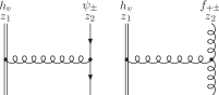
Figure 1: Diagrams contributing to the $2\to 2$-kernels in light cone gauge.

For the heavy-light $2\to 2$-kernels only the diagrams shown in figure 1 contribute nontrivially and there appears a single function $\mathcal{H}_{h}$ which depends solely on the conformal spin $j$ of the light degree of freedom:

$$\left[\mathcal{H}_{h}\mathcal{O}\right](z_{1},z_{2})=\int_{0}^{1}\dfrac{d\alpha}{\alpha}\left(\mathcal{O}(z_{1},z_{2})-\bar{\alpha}^{2j-1}\mathcal{O}(z_{1},z_{21}^{\alpha})\right)+\log(i\mu(z_{2}-z_{1})).$$ (75)

The results do not, except for a sign, depend on the chirality of the light degrees of freedom nor if one considers a $\psi$- or a $\chi$-spinor. They are given simply by multiplying $\mathcal{H}_{h}$ with the appropriate colour structure and adding the respective constants $\sigma_{q},\,\sigma_{g}$ and $\sigma_{h}$:

$$\mathbb{H}\,h^{i}_{v}(z_{1})f^{a}_{++}(z_{2}) = -2\left(t_{ii^{\prime}}^{b}\,t_{aa^{\prime}}^{b}\right)\left[\mathcal{H}_{h}-\sigma_{h}-\sigma_{g}\right]h_{v}^{i^{\prime}}(z_{1})f_{++}^{a^{\prime}}(z_{2}),$$ (76)

$$\mathbb{H}\,h^{i}_{v}(z_{1})f^{a}_{+-}(z_{2}) = -2\left(t_{ii^{\prime}}^{b}\,t_{aa^{\prime}}^{b}\right)\left[\mathcal{H}_{h}-\sigma_{h}-\sigma_{g}\right]h_{v}^{i^{\prime}}(z_{1})f_{+-}^{a^{\prime}}(z_{2}),$$ (77)

$$\mathbb{H}\,h^{i}_{v}(z_{1})\psi^{j}_{+}(z_{2}) = -2\left(t_{ii^{\prime}}^{b}\,t_{jj^{\prime}}^{b}\right)\left[\mathcal{H}_{h}-\sigma_{h}-\sigma_{q}\right]h_{v}^{i^{\prime}}(z_{1})\psi_{+}^{j^{\prime}}(z_{2}),$$ (78)

$$\mathbb{H}\,h^{i}_{v}(z_{1})\psi^{j}_{-}(z_{2}) = -2\left(t_{ii^{\prime}}^{b}\,t_{jj^{\prime}}^{b}\right)\left[\mathcal{H}_{h}-\sigma_{h}-\sigma_{q}\right]h_{v}^{i^{\prime}}(z_{1})\psi_{-}^{j^{\prime}}(z_{2}).$$ (79)

The form of (75) does not come unexpected. The first part resembles the contribution coming from light degrees of freedom seen in Braun:2009vc as well and the heavy quark just gives a contribution coming from the renormalisation of two intersecting Wilson-lines, one light-like and one time-like.

3.3 $2\to 3$-kernels

For the two $2\to 3$-kernels we calculated, we closely follow the notation of Braun:2009vc . Before we give the results let us recall some of the abbreviations used there.
In light cone gauge the one loop renormalisation of an operator $[X]_{R}(z_{1},z_{2})$ can in general be written as

$$\left[X\right]_{R}(z_{1},z_{2})=X_{B}(z_{1},z_{2})+\dfrac{\alpha_{s}}{4\pi\varepsilon}\left[\mathbb{H}^{(2\to 2)}X\right](z_{1},z_{2})+\dfrac{\alpha_{s}}{4\pi\varepsilon}\left[\mathbb{H}^{(2\to 3)}Y\right](z_{1},z_{2})$$ (80)

where $X_{B}(z_{1},z_{2})$ is the bare operator and the relevant $2\to 2$-kernels $\mathbb{H}^{(2\to 2)}$ have been given in the preceding section, though we would have to add the $\frac{1}{\varepsilon^{2}}$-poles here. We first consider the simpler case $X^{ij}(z_{1},z_{2})=h_{v}^{i}(z_{1})\psi^{j}_{-}(z_{2})$. It mixes with just a single operator

$$Y^{ija}=g(\mu\lambda)h_{v}^{i}(z_{1})\psi_{+}^{j}(z_{2})\bar{f}_{++}^{a}(z_{3})$$

and there are only two different colour structures for the three-particle counter term

$$\left[\mathbb{H}^{(2\to 3)}Y\right]^{ij}=\left\{f^{abc}t^{b}_{ii^{\prime}}t^{c}_{jj^{\prime}}\mathcal{H}_{1}+it^{b}_{ii^{\prime}}(t^{d}t^{b})_{jj^{\prime}}\mathcal{H}_{2}\right\}Y^{i^{\prime}j^{\prime}a},$$ (81)

which in light cone gauge follows from the Feynman-diagrams shown in figure 2 a).
For $X^{ia}(z_{1},z_{2})=h^{i}_{v}(z_{1})f^{a}_{+-}(z_{2})$ the calculation is more complicated, there are five diagrams (see figure 2 b)) contributing, it mixes with three different operators

$$Y^{iad}(z_{1},z_{2},z_{3}) = g(\mu\lambda)h^{i}_{v}(z_{1})f_{++}^{a}(z_{2})\bar{f}_{++}^{d}(z_{3}),$$

$$J^{ia}(z_{1},z_{2}) = g(\mu\lambda)h^{i}_{v}(z_{1})\left(\bar{\psi}_{+}(z_{2})t^{a}\psi_{+}(z_{2})+\chi_{+}(z_{2})t^{a}\bar{\chi}_{+}(z_{2})\right),$$

$$Z^{iab}(z_{1},z_{2},z_{3}) = g(\mu\lambda)h_{v}^{i}(z_{1})\left(\bar{\psi}_{+}(z_{2})t^{a}t^{b}\psi_{+}(z_{3})-\chi_{+}(z_{2})t^{b}t^{a}\bar{\chi}_{+}(z_{3})\right),$$

and there appear four different colour structures

$$\left[\mathbb{H}^{(2\to 3)}Y\right]^{ia} = \Big{(}\left\{f^{dbc}t^{b}_{ii^{\prime}}f^{aca^{\prime}}\mathcal{H}_{1}+i(t^{d}t^{b})_{ii^{\prime}}f^{aba^{\prime}}\mathcal{H}_{2}\right\}Y^{i^{\prime}a^{\prime}d}$$ (83)

$$+ t_{ii^{\prime}}^{b}f^{aba^{\prime}}\tilde{\mathcal{H}}_{1}J^{i^{\prime}a^{\prime}}+t_{ii^{\prime}}^{b}\tilde{\mathcal{H}}_{2}Z^{i^{\prime}ab}\Big{)}.$$

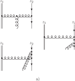
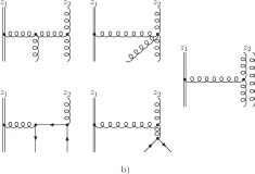
Figure 2: Wilson-lines are omitted since light cone gauge $n\cdot A=0$ is used. a) Single diagram contributing to kernels (84). b) Diagrams contributing to kernels (85)

The results are given below where a comparison with the results for the counterterms of $\psi_{+}\otimes\psi_{-}$ and $f_{+-}\otimes\psi_{+}$ from Braun:2009vc shows that they coincide if one substitutes $h_{v}\to\psi_{+}$. This indicates that the $2\to 3$-mixing is solely governed by the twist of the light degrees of freedom. In addition we could not find any extraordinary mixing under renormalisation due to the heavy quark.

1. $X^{ij}(z_{1},z_{2})=h_{v}^{i}(z_{1})\psi_{-}^{j}(z_{2})$.
   As stated there is only a single operator $Y^{ijd}(z_{1},z_{2},z_{3})=g(\mu\lambda)h^{i}_{v}(z_{1})\psi^{j}_{+}(z_{2})\bar{f}^{d}_{++}(z_{3})$ needed in this case. The two kernels appearing in (81) are given by:

   $$\left[\mathcal{H}_{1}Y\right](z_{1},z_{2}) = z_{12}^{2}\int_{0}^{1}d\alpha\int_{0}^{\bar{\alpha}}d\beta\,\beta\,Y(z_{1},z_{21}^{\alpha},z_{12}^{\beta}),$$

   $$\left[\mathcal{H}_{2}Y\right](z_{1},z_{2}) = z_{12}^{2}\int_{0}^{1}d\alpha\int_{\bar{\alpha}}^{1}d\beta\dfrac{\bar{\alpha}\bar{\beta}}{\alpha}\,Y(z_{1},z_{21}^{\alpha},z_{12}^{\beta}).$$ (84)

2. $X^{ia}(z_{1},z_{2})=h_{v}^{i}(z_{1})f^{a}_{+-}(z_{2})$.
   Here the three operators from (LABEL:eq:op-23) contribute with colour structures and kernels specified as in (83). The latter can be written as

   $$\left[\mathcal{H}_{1}Y\right](z_{1},z_{2}) = z_{12}^{2}\int_{0}^{1}d\alpha\int_{0}^{\bar{\alpha}}d\beta\,\bar{\alpha}\beta\,Y(z_{1},z_{21}^{\alpha},z_{12}^{\beta}),$$

   $$\left[\mathcal{H}_{2}Y\right](z_{1},z_{2}) = z_{12}^{2}\int_{0}^{1}d\alpha\int_{\bar{\alpha}}^{1}d\beta\dfrac{\bar{\alpha}^{2}\bar{\beta}}{\alpha}\,Y(z_{1},z_{21}^{\alpha},z_{12}^{\beta}),$$

   $$\left[\tilde{\mathcal{H}}_{1}J\right](z_{1},z_{2}) = -z_{12}\int_{0}^{1}d\alpha\,\bar{\alpha}^{2}\,J(z_{1},z_{21}^{\alpha}),$$

   $$\left[\tilde{\mathcal{H}}_{2}Z\right](z_{1},z_{2}) = z_{12}\int_{0}^{1}d\alpha\int_{\bar{\alpha}}^{1}d\beta\dfrac{\bar{\beta}}{\beta}\,Z(z_{1},z_{12}^{\alpha},z_{21}^{\beta}),$$ (85)

   where for brevities sake we omitted all colour indices.

4 Constraints from conformal symmetry and
breaking of scale invariance due to the heavy quark

As was seen in section 3 the $2\to 2$-kernels are functions of only one variable $z_{2}-z_{1}$ so for simplicity we use here $z_{1}=0$ and $z_{2}=t$. To use constraints from conformal symmetry we first have to determine the behaviour of the heavy quarks under conformal transformations. The heavy quark can be written as a time-like Wilson-line times a sterile scalar field Korchemsky:1991zp :

$$h_{v}(0)=P\exp\left\{ig_{s}\int_{-\infty}^{0}d\alpha\,v^{\mu}A_{\mu}(\alpha v)\right\}\phi(-\infty).$$ (86)

There are two conformal transformations that map the respective time-like Wilson-line onto itself: the special conformal transformation along the $v$-direction where $v_{\mu}=\frac{1}{2}(n_{\mu}+\tilde{n}_{\mu})$ and the dilatation, for definitions see section 2.4. The generators of these transformations are given by

$$i\left[v\cdot\mathbf{K},\Phi(x)\right] = \left[2v\cdot xx\cdot\partial-x^{2}v\cdot\partial+2lv\cdot x-2v_{\mu}x_{\nu}\Sigma^{\mu\nu}\right]\Phi(x)=v\cdot K\,\Phi(x),$$

$$i\left[\mathbf{D},\Phi(x)\right] = \left[x\cdot\partial+l\right]\Phi(x)=D\,\Phi(x),$$ (87)

with

$$i\left[v\cdot\mathbf{K},\mathbf{D}\right]=-v\cdot\mathbf{K}.$$

As introduced in section 2.4, $\Phi$ is either a scalar, a spinor or a vector field, $l$ is the canonical dimension of the field and $\Sigma^{\mu\nu}$ is the generator of spin rotations. For fields living on the light cone

$$\Phi(z)=\Phi(zn),\quad n^{2}=0$$

the two generators take on an especially simple form:

$$i\left[v\cdot\mathbf{K},\Phi(z)\right] = (2z^{2}\partial_{z}+4jz)\Phi(z)=v\cdot K\,\Phi(z),$$ (88)

$$i\left[\mathbf{D},\Phi(z)\right] = (z\partial_{z}+l)\Phi(z)=D\,\Phi(z),$$ (89)

where $j=\frac{1}{2}(l+s)$ with $\Sigma_{+-}\Phi(z)=s\Phi(z)$ is the conformal spin of the light field. In particular $v\cdot\mathbf{K}$ is reduced to $\tilde{n}\cdot\mathbf{K}$ since a special conformal transformation in the $n$-direction has no effect altogether. Additionally there is no interchange of plus and minus components of the fields under $v\cdot\mathbf{K}$ since such terms would be proportional to transverse coordinates. This can be seen explicitly if one writes down the generator of special conformal transformations in spinor notation, $v\cdot\mathbf{K}=\mathbf{K}_{1\dot{1}}+\mathbf{K}_{2\dot{2}}$:

$$i\left[\mathbf{K}_{\alpha\dot{\alpha}},\psi_{\beta}\right](x) = \left(x_{\alpha\dot{\gamma}}x_{\gamma\dot{\alpha}}\partial^{\gamma\dot{\gamma}}+4x_{\alpha\dot{\alpha}}\right)\psi_{\beta}(x)-2x_{\beta\dot{\alpha}}\psi_{\alpha},$$ (90)

$$i\left[\mathbf{K}_{\alpha\dot{\alpha}},f_{\beta\delta}\right](x) = \left(x_{\alpha\dot{\gamma}}x_{\gamma\dot{\alpha}}\partial^{\gamma\dot{\gamma}}+6x_{\alpha\dot{\alpha}}\right)f_{\beta\delta}(x)-2x_{\beta\dot{\alpha}}f_{\alpha\delta}-2x_{\delta\dot{\alpha}}f_{\alpha\beta}.$$ (91)

Heavy-light light ray operators therefore behave in a well defined way under this transformations. What happens after renormalisation? From the explicit form of the renormalisation kernels (75) and the differential operators (88), (89) the following commutation relations for $\mathcal{H}$ with $D$ and $v\cdot K$ are derived:

$$\left[D,\mathcal{H}_{h}\right]\mathcal{O}(t) = \mathcal{O}(t),$$ (92)

$$\left[v\cdot K,\mathcal{H}_{h}\right]\mathcal{O}(t) = 0.$$ (93)

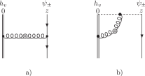
Figure 3: Feynman-diagrams which are responsible for the breaking of the conformal invariance in a) light cone gauge b) Feynman-gauge. A change of the light degrees of freedom does not alter the calculation substantially in light cone gauge. The cross denotes the insertion of $(D-4)\int d^{D}x\,G_{\mu\rho}^{a}G^{a\mu\rho}(x)$ or $2(D-4)\int d^{D}x\,x^{\nu}G_{\mu\rho}^{a}G^{a\mu\rho}(x)$ .

They show that the variation of the operator under dilatation and its renormalisation do not commute which means that in contrast to the case of pure massless QCD, where scale invariance is broken at one loop order only by finite terms and therefore the renormalisation of light-light light ray operators is not affected to this order, the inclusion of an effective heavy quark gives a contribution that breaks scale invariance already at the level of the one loop counterterms. We will proceed to show that this phenomenon can be directly traced back to the cusp at $z=0$ in the time-like Wilson-line representing the effective heavy quark and the light-like Wilson-lines included for gauge invariance. In Derkachov:2010zza a simple proof was given that the one loop counterterms inherit conformal symmetry from the Lagrange-density. We will apply their results to the case at hand. Let $\mathcal{O}(\Phi)$ be a two-particle operator with an effective heavy quark and $\Delta\mathcal{O}(\Phi)$ be its counterterm. Therefore Green-functions with an insertion of $\mathcal{O}(\Phi)+\Delta\mathcal{O}(\Phi)$ or equivalent the path integral

$$G_{\mathcal{O}}(\lambda)=\int[D\Phi]\exp\left\{-S_{R}+i\int d^{4}x\,\lambda\,\Phi\right\}(\mathcal{O}(\Phi)+\Delta\mathcal{O}(\Phi))$$ (94)

are finite. Here $S_{R}$ denotes the renormalised action of QCD and HQET while $\Phi$ is any one of the relevant fields $A_{\mu},\,\psi,\,h_{v},\ldots$ and $\lambda$ the respective source. Making a change of variables $\Phi\to\Phi^{\prime}=\Phi+\delta_{\alpha}\Phi$ where $\delta_{\alpha}=\alpha\delta_{D}\Phi=\alpha\,i[\mathbf{D},\Phi]$ does not change the path integral and leads to the relation:

$$\int[D\Phi]\exp\left\{iS_{R}+i\int d^{4}x\,\lambda\,\Phi\right\}(\delta_{\alpha}\mathcal{O}(\Phi)+\delta_{\alpha}\Delta\mathcal{O}(\Phi))$$ (95)

$$=\int[D\Phi]\exp\left\{iS_{R}+i\int d^{4}x\,\lambda\,\Phi\right\}\left(\delta_{\alpha}S_{R}-i\int d^{4}x\lambda\delta_{\alpha}\Phi\right)\times(\mathcal{O}(\Phi)+\Delta\mathcal{O}(\Phi)).$$ (96)

As stated, equation (92) implies that the counterterm of the variation of the operator is not identical to the varied counterterm

$$\Delta(\delta_{\alpha}\mathcal{O}(\Phi))\neq\delta_{\alpha}(\Delta\mathcal{O}(\Phi)),$$ (97)

for $\delta_{\alpha}=\alpha\delta_{D}$ and we proceed to show that this follows directly from the right hand side of equation (96). The term proportional to the sources $\lambda$ is finite at one loop order Derkachov:2010zza , therefore the only relevant term is

$$\int[D\Phi]\exp\left\{iS_{R}+i\int d^{4}x\,\lambda\,\Phi\right\}\delta_{\alpha}S_{R}\times\mathcal{O}(\Phi).$$ (98)

Using that the variation under (global) dilatation of the action is given by (40), (42), see also Braun:2003rp

$$\delta_{D}S = \int d^{D}x\Delta_{D}(x),$$ (99)

$$= \int d^{D}x(D-4)G_{\mu\nu}^{a}G^{a\mu\nu}(x)+\mathcal{O}(\alpha_{s}),$$

where we omitted the total derivative of $\mathcal{O}_{B\lambda}$, one can calculate the integral (98) at one loop level. In light cone gauge there is just the exchange diagram with an insertion of (99). One needs an $\frac{1}{\varepsilon^{2}}$-pole so that after the multiplication with $D-4$ from (99) there remains a divergent part which would proof (97). The relevant contribution comes from the additional term in the gluon propagators and that part of (99) where the derivatives in the field-strength tensor cancel one of the denominators. For the example in figure 3 a) these contributions to (98) amount to

$$\delta_{\alpha}=\alpha\,\delta_{D}:\quad C_{F}g_{s}^{2}(D-4)\int\dfrac{d^{D}l}{(2\pi)^{D}}\dfrac{1}{l_{+}\,v\cdot l\,(k-l)^{2}}e^{-i(k_{+}-l_{+})z}$$ (100)

which after integration confirms (92). The calculation does not substantially depend on the light degree of freedom which is explicitly seen if one does the same derivation in Feynman-gauge. Analysing the relevant diagrams only those of figure 3 b) contribute which clearly shows that only the colour structure of the result depends on the light degree of freedom and as anticipated the breaking of scale invariance comes due to the additional UV-renormalisation from the cusp in the two Wilson-lines Korchemsky:1987wg , where one is light-like included for gauge-invariance and the other is time-like and is representing the effective heavy quark. An explicit calculation again reproduces the results in equation (92) though the colour structures only match for gauge invariant operators. It should be noted that these $\frac{1}{\varepsilon^{2}}$-poles appear only for the two-particle counterterms while the three-particle terms are unaffected. A fact that supports the assumption that the mixing with three-particle operators is constrained by the transformation properties with respect to the conformal group of the light degrees of freedom and which probably could be further exploited.
The same computation as for the dilatation can be done for the case of $v\cdot\mathbf{K}$ but here the additional $x^{\nu}$ in $\delta_{K}S$, see (43), gives an extra propagator denominator, so that the relevant integral amounts to

$$\delta_{\alpha}=\alpha\,\delta_{v\cdot K}:\quad 2C_{F}g_{s}^{2}(D-4)\int\dfrac{d^{D}l}{(2\pi)^{D}}\dfrac{1}{l_{+}}\left[\dfrac{1}{(v\cdot l)^{2}\,(k-l)^{2}}+\dfrac{1}{(k-l)^{4}}\right]e^{-i(k_{+}-l_{+})z},$$ (101)

which gives only a finite contribution and in this way confirms (93).
Another interesting point following from this considerations is that the $2\to 2$ evolution kernels are fixed up to a constant by the constraints (92) and (93). It is not possible to construct a finite integral kernel $\mathcal{H}$ of a single variable which commutes with both $D$ and $v\cdot K$ except for a constant and therefore it is not possible to write down an evolution kernel that fulfils the constraints (92) and (93) that differs from (75) by more than said constant. This can be understood in the following way: An integral kernel of a single variable that is invariant under dilatations has the form

$$\left[\mathcal{H}\mathcal{O}\right](z)=A\int_{0}^{z}\dfrac{dt}{z}\,f\left(\dfrac{t}{z}\right)\,\mathcal{O}(t)+B\mathcal{O}(z),$$ (102)

where $f$ is a generic function that gives a finite integral and $A$ and $B$ are arbitrary constants. This can be written in the more familiar way

$$\left[\mathcal{H}\mathcal{O}\right](z)=A\int_{0}^{1}d\alpha\,f\left(\bar{\alpha}\right)\,\mathcal{O}(\bar{\alpha}z)+B\mathcal{O}(z).$$ (103)

Now taking the differential operator for $v\cdot K$ (88) and calculating the commutator $[v\cdot K,\mathcal{H}]\mathcal{O}(t)$ one gets the following differential equation for $f(\bar{\alpha})$:

$$\alpha\bar{\alpha}\dfrac{d}{d\alpha}f(\bar{\alpha})+(1-2\alpha(1-j))f(\bar{\alpha})=0,$$ (104)

with the boundary conditions

$$\lim_{\alpha\to 1}\alpha\bar{\alpha}f(\bar{\alpha})=0,\qquad\lim_{\alpha\to 0}\alpha\bar{\alpha}f(\bar{\alpha})=0.$$

The solution to (104)

$$f(\bar{\alpha})=C\dfrac{\bar{\alpha}^{2j-1}}{\alpha}$$ (105)

violates the boundary conditions and therefore only a constant can commute with both $D$ and $v\cdot K$. Taking this argument a little further one can use that (100) and therefore (92) and (93) are a general feature of the renormalisation of heavy-light operators and then construct $\mathcal{H}_{h}$ up to a constant by exploiting these constraints. In light cone gauge the term violating scale invariance has the same colour factor as the rest of the renormalisation kernel. We add a $\log(i\mu z)$-term to (103) which then is the most general expression that fulfils (92). Solving the constraint (93) then amounts to solving (104) with the changed boundary condition

$$\lim_{\alpha\to 0}\alpha\bar{\alpha}f(\bar{\alpha})=-1,$$

where (105) is now a viable and therefore unique solution, except for a constant. With the regularised $f(\bar{\alpha})$

$$f(\bar{\alpha})=\left(-\dfrac{\bar{\alpha}^{2j-1}}{\alpha}\right)_{+},$$

where

$$\int_{0}^{1}d\alpha\left(-\dfrac{\bar{\alpha}^{2j-1}}{\alpha}\right)_{+}\mathcal{O}(\bar{\alpha}z)=\int_{0}^{1}d\alpha\dfrac{\bar{\alpha}^{2j-1}}{\alpha}(\mathcal{O}(z)-\mathcal{O}(\bar{\alpha}z))$$

we then get (75) apart for an unconstrained constant.

5 Applications

Matrix elements of heavy-light light ray operators are used in a wide array of factorisation theorems for exclusive decays. In this section we demonstrate a few important examples, where our results might be of use.

5.1 B-meson distribution amplitudes

The most prominent applications are without any doubt the distribution amplitudes of the B-meson. The two two-particle distribution amplitudes $\tilde{\phi}_{B}^{+},\,\tilde{\phi}_{B}^{-}$ are defined by the following matrix element:

$$\langle 0|\bar{q}_{\beta}(z)[z,0](h_{v})_{\alpha}(0)|B(p)\rangle=-i\frac{\hat{f}_{B}(\mu)}{4}\left[(1+\mathchoice{\ooalign{$\hfil\displaystyle\mkern 0.0mu/\hfil$\crcr$\displaystyle v$}}{\ooalign{$\hfil\textstyle\mkern 0.0mu/\hfil$\crcr$\textstyle v$}}{\ooalign{$\hfil\scriptstyle\mkern 0.0mu/\hfil$\crcr$\scriptstyle v$}}{\ooalign{$\hfil\scriptscriptstyle\mkern 0.0mu/\hfil$\crcr$\scriptscriptstyle v$}})\left(\tilde{\phi}_{B}^{+}(t)+\frac{\mathchoice{\ooalign{$\hfil\displaystyle\mkern 0.0mu/\hfil$\crcr$\displaystyle z$}}{\ooalign{$\hfil\textstyle\mkern 0.0mu/\hfil$\crcr$\textstyle z$}}{\ooalign{$\hfil\scriptstyle\mkern 0.0mu/\hfil$\crcr$\scriptstyle z$}}{\ooalign{$\hfil\scriptscriptstyle\mkern 0.0mu/\hfil$\crcr$\scriptscriptstyle z$}}}{2t}[\tilde{\phi}_{B}^{-}(t)-\tilde{\phi}_{B}^{+}(t)]\right)\gamma_{5}\right]_{\alpha\beta},$$ (106)

with $t=v\cdot z$ and $z^{2}=0$. Inserting $\hfil\textstyle\mkern 0.0mu/\hfil$ $\textstyle n$ or $\tilde{\mathchoice{\ooalign{$\hfil\displaystyle\mkern 0.0mu/\hfil$\crcr$\displaystyle n$}}{\ooalign{$\hfil\textstyle\mkern 0.0mu/\hfil$\crcr$\textstyle n$}}{\ooalign{$\hfil\scriptstyle\mkern 0.0mu/\hfil$\crcr$\scriptstyle n$}}{\ooalign{$\hfil\scriptscriptstyle\mkern 0.0mu/\hfil$\crcr$\scriptscriptstyle n$}}}$ one can project on $\tilde{\phi}_{B}^{+}$ or $\tilde{\phi}_{B}^{-}$, respectively. The relevant operators in spinor notation are then

$$\mathcal{O}_{+}(0,z)=S(h^{i}_{v}\otimes\psi^{j}_{+}),\qquad\mathcal{O}_{-}(0,z)=S(h^{i}_{v}\otimes\psi^{j}_{-}),$$ (107)

where $S=\delta_{ij}$. By multiplying equation (78) with $\delta_{ij}$, setting $z_{1}=0$, $z_{2}=z$, and correcting for the renormalisation of the B-meson decay constant in HQET one recovers for $\phi_{B}^{+}$ the result of Braun:2003wx ; Kawamura:2010tj . After a Fourier-transformation the result of Lange:2003ff follows. The same can be done for $\phi_{B}^{-}$ by using equations (79) and (84). A Fourier-transformation confirms the results of Bell:2008er ; DescotesGenon:2009hk . Some care has to be taken in Fourier-transforming the $\log$-term:

$$\dfrac{1}{2\pi}\int_{-\infty}^{+\infty}dte^{i\omega t}\log(i\mu(t-i\epsilon))\mathcal{O}_{\pm}(0,t)$$

$$=\dfrac{i}{2\pi}\int_{0}^{\infty}d\omega^{\prime}\left\{\dfrac{1}{\omega^{\prime}-\omega-i\epsilon}\log\dfrac{\omega^{\prime}-\omega-i\epsilon}{\mu}\right.$$

$$\left.-\dfrac{1}{\omega^{\prime}-\omega+i\epsilon}\log\dfrac{\omega^{\prime}-\omega+i\epsilon}{\mu}\right\}\mathcal{O}_{\pm}(\omega^{\prime},\mu)$$

$$=-\log\dfrac{\mu}{\omega}\mathcal{O}_{\pm}(\omega,\mu)-\int_{0}^{\infty}d\omega^{\prime}\left(\dfrac{\Theta(\omega^{\prime}-\omega)}{\omega^{\prime}-\omega}\right)_{+}\mathcal{O}_{\pm}(\omega^{\prime},\mu),$$ (108)

where we define the $+$-distribution in the usual way

$$\int d\omega^{\prime}\left(f(\omega,\omega^{\prime})\right)_{+}\,g(\omega^{\prime})=\int d\omega^{\prime}f(\omega,\omega^{\prime})g(\omega^{\prime})-g(\omega)\int d\rho f(\rho,\omega).$$

All other terms do not need any special treatment. In principle, taking our results, it does not pose a problem to construct the renormalisation of many-particle distribution amplitudes with an arbitrary amount of quarks and transverse gluons but here we just want to comment on two three-particle distribution amplitudes. They were defined in Kawamura:2001jm via the following matrix element: (for a more general approach see Geyer:2005fb ; Geyer:2007yh )

$$\langle 0|\bar{q}_{\beta}(z)[z,uz]gG_{\mu\nu}(uz)z^{\nu}[uz,0](h_{v})_{\alpha}(0)|B(p)\rangle$$

$$=\frac{\hat{f}_{B}(\mu)M}{4}\left[(1+\mathchoice{\ooalign{$\hfil\displaystyle\mkern 0.0mu/\hfil$\crcr$\displaystyle v$}}{\ooalign{$\hfil\textstyle\mkern 0.0mu/\hfil$\crcr$\textstyle v$}}{\ooalign{$\hfil\scriptstyle\mkern 0.0mu/\hfil$\crcr$\scriptstyle v$}}{\ooalign{$\hfil\scriptscriptstyle\mkern 0.0mu/\hfil$\crcr$\scriptscriptstyle v$}})\left[(v_{\mu}\mathchoice{\ooalign{$\hfil\displaystyle\mkern 0.0mu/\hfil$\crcr$\displaystyle z$}}{\ooalign{$\hfil\textstyle\mkern 0.0mu/\hfil$\crcr$\textstyle z$}}{\ooalign{$\hfil\scriptstyle\mkern 0.0mu/\hfil$\crcr$\scriptstyle z$}}{\ooalign{$\hfil\scriptscriptstyle\mkern 0.0mu/\hfil$\crcr$\scriptscriptstyle z$}}-t\gamma_{\mu})\left(\tilde{\Psi}_{A}(t,u)-\tilde{\Psi}_{V}(t,u)\right)-i\sigma_{\mu\nu}z^{\nu}\tilde{\Psi}_{V}(t,u)\right.\right.$$ (125)

$$\left.\left.\qquad\qquad\qquad\qquad-z_{\mu}\tilde{X}_{A}(t,u)+\frac{z_{\mu}\mathchoice{\ooalign{$\hfil\displaystyle\mkern 0.0mu/\hfil$\crcr$\displaystyle z$}}{\ooalign{$\hfil\textstyle\mkern 0.0mu/\hfil$\crcr$\textstyle z$}}{\ooalign{$\hfil\scriptstyle\mkern 0.0mu/\hfil$\crcr$\scriptstyle z$}}{\ooalign{$\hfil\scriptscriptstyle\mkern 0.0mu/\hfil$\crcr$\scriptscriptstyle z$}}}{t}\tilde{Y}_{A}(t,u)\right]\gamma_{5}\right]_{\alpha\beta}.$$ (134)

The combinations $\tilde{\Psi}_{A}-\tilde{\Psi}_{V}$ and $\tilde{\Psi}_{A}+\tilde{\Psi}_{V}$ can be identified as

$$\mathcal{O}_{A-V}(0,uz,z)=S(h^{i}_{v}\otimes f^{a}_{++}\otimes\bar{\psi}^{j}_{+}),\qquad\mathcal{O}_{A+V}(0,uz,z)=S(h^{i}_{v}\otimes\bar{f}^{a}_{++}\otimes\bar{\psi}^{j}_{-}),$$ (135)

with $S=t_{ij}^{a}$, while $\tilde{\Psi}_{A}$ and $\tilde{\Psi}_{V}$ are given as sum or difference of these operators and therefore cannot be associated with a well defined twist for the light degrees of freedom. Using the results from Braun:2009vc and equations (76), (78) it is easy to construct the renormalisation of this distribution amplitudes. We confirm the results of Offen:2009mt for $\Psi_{A}-\Psi_{V}$ after a Fourier-transformation.

5.2 $\Lambda_{b}$ distribution amplitudes

The $\Lambda_{b}$ distribution amplitudes are defined as matrix elements of non-local light ray operators built of an effective heavy quark and two light quarks, see e.g. Ball:2008fw :

$$\epsilon^{ijk}\langle 0|\left(u^{T\,i}(t_{1}n)C\gamma_{5}\mathchoice{\ooalign{$\hfil\displaystyle\mkern 0.0mu/\hfil$\crcr$\displaystyle n$}}{\ooalign{$\hfil\textstyle\mkern 0.0mu/\hfil$\crcr$\textstyle n$}}{\ooalign{$\hfil\scriptstyle\mkern 0.0mu/\hfil$\crcr$\scriptstyle n$}}{\ooalign{$\hfil\scriptscriptstyle\mkern 0.0mu/\hfil$\crcr$\scriptscriptstyle n$}}d^{j}(t_{2}n)\right)h_{v}^{k}(0)|\Lambda(v)\rangle = f_{\Lambda}^{(2)}\Psi_{2}(t_{1},t_{2})\Lambda(v),$$ (144)

$$\epsilon^{ijk}\langle 0|\left(u^{T\,i}(t_{1}n)C\gamma_{5}d^{j}(t_{2}n)\right)h_{v}^{k}(0)|\Lambda(v)\rangle = f_{\Lambda}^{(1)}\Psi^{s}_{3}(t_{1},t_{2})\Lambda(v),$$

$$\epsilon^{ijk}\langle 0|\left(u^{T\,i}(t_{1}n)C\gamma_{5}i\sigma_{\tilde{n}n}d^{j}(t_{2}n)\right)h_{v}^{k}(0)|\Lambda(v)\rangle = f_{\Lambda}^{(1)}\Psi^{\sigma}_{3}(t_{1},t_{2})\Lambda(v),$$

$$\epsilon^{ijk}\langle 0|\left(u^{T\,i}(t_{1}n)C\gamma_{5}\tilde{\mathchoice{\ooalign{$\hfil\displaystyle\mkern 0.0mu/\hfil$\crcr$\displaystyle n$}}{\ooalign{$\hfil\textstyle\mkern 0.0mu/\hfil$\crcr$\textstyle n$}}{\ooalign{$\hfil\scriptstyle\mkern 0.0mu/\hfil$\crcr$\scriptstyle n$}}{\ooalign{$\hfil\scriptscriptstyle\mkern 0.0mu/\hfil$\crcr$\scriptscriptstyle n$}}}d^{j}(t_{2}n)\right)h_{v}^{k}(0)|\Lambda(v)\rangle = f_{\Lambda}^{(2)}\Psi_{4}(t_{1},t_{2})\Lambda(v).$$ (153)

$\Lambda(v)$ is a Dirac-spinor fulfilling $\mathchoice{\ooalign{$\hfil\displaystyle\mkern 0.0mu/\hfil$\crcr$\displaystyle v$}}{\ooalign{$\hfil\textstyle\mkern 0.0mu/\hfil$\crcr$\textstyle v$}}{\ooalign{$\hfil\scriptstyle\mkern 0.0mu/\hfil$\crcr$\scriptstyle v$}}{\ooalign{$\hfil\scriptscriptstyle\mkern 0.0mu/\hfil$\crcr$\scriptscriptstyle v$}}\Lambda(v)=\Lambda(v)$ where non-relativistic normalisation $\bar{\Lambda}\Lambda=1$ is assumed, $\sigma_{\tilde{n}n}=\sigma_{\mu\nu}\tilde{n}^{\mu}n^{\nu}$, $C$ is the charge conjugation matrix which in spinor representation looks like

$$C=\left(\begin{array}[]{cc}-\epsilon_{\alpha\beta}&0\\ 0&-\epsilon_{\dot{\alpha}\dot{\beta}}\end{array}\right)$$ (154)

and the subscripts refer to the twist of the light diquark operator. $\Psi_{3}^{\sigma}$ is antisymmetric under interchange of the light quark coordinates while the others are symmetric. In spinor notation the relevant operators are

$$\mathcal{O}_{2}(t_{1},t_{2}) = \epsilon^{ijk}\left(\psi_{+}^{i}(t_{1})\,\bar{\chi}_{+}^{j}(t_{2})\,h_{v}^{k}(0)\right),$$

$$\mathcal{O}_{3}(t_{1},t_{2}) = \epsilon^{ijk}\left(\psi_{+}^{i}(t_{1})\,\psi_{-}^{j}(t_{2})\,h_{v}^{k}(0)\right),$$

$$\mathcal{O}_{4}(t_{1},t_{2}) = \epsilon^{ijk}\left(\psi_{-}^{i}(t_{1})\,\bar{\chi}_{-}^{j}(t_{2})\,h_{v}^{k}(0)\right).$$ (155)

Using the results (78) for $h_{v}\otimes\psi_{+}$ and $\psi_{+}\otimes\bar{\psi}_{+}$ from Braun:2009vc and correcting for the renormalisation of $f_{\Lambda}^{(2)}$ we recover the expressions of Ball:2008fw but we can extend their result to the $\Psi_{3}$ case by using the necessary expressions for

$$h_{v}\otimes\psi_{-},\quad h_{v}\otimes\psi_{+},\quad\psi_{+}\otimes\psi_{-},$$

from equations (79), (84) and from Braun:2009vc . We will give a short outline of the calculation as an example of possible applications. The relevant kernel from Braun:2009vc is

$$\left[\mathbb{H}\,\psi_{+}^{i}\,\psi_{-}^{j}\right](z_{1},z_{2}) = -2t^{b}_{ii^{\prime}}t^{b}_{jj^{\prime}}\left[\left[\hat{\mathcal{H}}\,\psi_{+}^{i^{\prime}}\psi_{-}^{j^{\prime}}\right](z_{1},z_{2})+2\sigma_{q}\psi_{+}^{i^{\prime}}(z_{1})\psi_{-}^{j^{\prime}}(z_{2})\right.$$ (156)

$$+ \left.\left[\mathcal{H}_{21}^{e,1}\,\psi_{-}^{i^{\prime}}\psi_{+}^{j^{\prime}}\right](z_{1},z_{2})\right]$$

with

$$\left[\hat{\mathcal{H}}\varphi\right](z_{1},z_{2}) = \int_{0}^{1}d\alpha\left(2\varphi(z_{1},z_{2})-\bar{\alpha}^{2j_{1}-1}\varphi(z_{12}^{\alpha},z_{2})-\bar{\alpha}^{2j_{2}-1}\varphi(z_{1},z_{21}^{\alpha})\right),$$ (157)

$$\left[\mathcal{H}_{21}^{e,k}\varphi\right](z_{1},z_{2}) = \int_{0}^{1}d\alpha\,\alpha^{2j_{1}-k-1}\alpha^{k-1}\varphi(z_{12}^{\alpha},z_{2}).$$ (158)

After some simple colour algebra one can add up all necessary expressions resulting in the $3\to 3$ evolution of $\mathcal{O}_{3}$:

$$\left[\mathbb{H}^{(3\to 3)}\mathcal{O}_{3}\right] = \dfrac{\alpha_{s}}{2\pi}C_{F}\epsilon^{ijk}\left[\int_{0}^{1}d\alpha\left(2\psi^{i}_{+}(z_{1})\psi^{j}_{-}(z_{2})-\bar{\alpha}\psi^{i}_{+}(z_{12}^{\alpha})\psi^{j}_{-}(z_{2})-\psi^{i}_{+}(z_{1})\psi^{j}_{-}(z_{21}^{\alpha})\right)h_{v}^{k}(0)\right.$$ (159)

$$+ \psi_{+}^{i}(z_{1})\left\{\int_{0}^{1}d\alpha\left(\psi_{-}^{j}(z_{2})h_{v}^{k}(0)-\psi_{-}^{j}(\bar{\alpha}z_{2})h_{v}^{k}(0)\right)+\log(i\mu\,z_{2})\psi_{-}^{j}(z_{2})h_{v}^{k}(0)\right\}$$

$$+ \int_{0}^{1}d\alpha\left(\psi^{i}_{+}(z_{1})\psi_{-}^{j}(z_{2})h_{v}^{k}(0)-\bar{\alpha}\psi_{+}^{i}(\bar{\alpha}z_{1})\psi_{-}^{j}(z_{2})h_{v}^{k}(0)\right)-4\psi_{+}^{i}(z_{1})\psi_{-}^{j}(z_{2})h_{v}^{k}(0)$$

$$+ \log(i\mu\,z_{1})\psi_{+}^{i}(z_{1})\psi_{-}^{j}(z_{2})h_{v}^{k}(0)+\left.\int_{0}^{1}d\alpha\,\psi_{-}^{i}(z_{21}^{\alpha})\psi_{+}^{j}(z_{1})h_{v}^{k}(0)\right].$$

The mixing with four particle operators is in this case completely governed by the kernels (84) and comparatively short:

$$\left[\mathbb{H}^{(3\to 4)}\mathcal{O}_{3}\right] = \dfrac{\alpha_{s}}{2\pi}\epsilon^{ijk}\left[\psi_{+}^{i}(z_{1})\left\{f^{abc}t^{b}_{jj^{\prime}}t^{c}_{kk^{\prime}}z_{2}^{2}\int_{0}^{1}d\alpha\int_{0}^{\bar{\alpha}}d\beta\,\beta\,\psi_{+}^{j^{\prime}}(\bar{\alpha}z_{2})\bar{f}_{++}^{a}(\beta z_{2})\right.\right.$$ (160)

$$+ \left.i(t^{a}t^{b})_{jj^{\prime}}t^{b}_{kk^{\prime}}z_{2}^{2}\int_{0}^{1}d\alpha\int_{\bar{\alpha}}^{1}d\beta\dfrac{\bar{\alpha}\bar{\beta}}{\alpha}\psi_{+}^{j^{\prime}}(\bar{\alpha}z_{2})\bar{f}_{++}^{a}(\beta z_{2})\right\}h_{v}^{k^{\prime}}(0)$$

$$+ \psi_{+}^{i^{\prime}}(z_{1})\left\{f^{abc}t^{b}_{ii^{\prime}}t^{c}_{jj^{\prime}}z_{12}^{2}\int_{0}^{1}d\alpha\int_{0}^{\bar{\alpha}}d\beta\,\beta\,\psi_{+}^{j^{\prime}}(z_{21}^{\alpha})\bar{f}_{++}^{a}(z_{12}^{\beta})\right.$$

$$+ \left.\left.i(t^{a}t^{b})_{jj^{\prime}}t^{b}_{ii^{\prime}}z_{12}^{2}\int_{0}^{1}d\alpha\int_{\bar{\alpha}}^{1}d\beta\dfrac{\bar{\alpha}\bar{\beta}}{\alpha}\psi_{+}^{j^{\prime}}(z_{12}^{\alpha})\bar{f}_{++}^{a}(z_{21}^{\beta})\right\}h_{v}^{k}(0)\right].$$

As one can see, the pattern is similar as in the twist 3 pseudoscalar meson case. There the operators

$$\mathcal{O}^{1}_{3}(z_{1},z_{2})=\chi_{+}(z_{1})\psi_{-}(z_{2}),\quad\mathcal{O}^{2}_{3}(z_{1},z_{2})=\chi_{-}(z_{1})\psi_{+}(z_{2}),\quad\mathcal{O}^{3}_{3}(z_{1},z_{2},z_{3})=\chi_{+}(z_{1})\bar{f}_{++}(z_{2})\psi_{+}(z_{3})$$

build a closed set under renormalisation. Here we have

$$\mathcal{O}^{1}_{3}(t_{1},t_{2}) = \psi_{+}(t_{1})\,\psi_{-}(t_{2})\,h_{v}(0),$$

$$\mathcal{O}^{2}_{3}(t_{1},t_{2}) = \psi_{-}(t_{1})\,\psi_{+}(t_{2})\,h_{v}(0),$$

$$\mathcal{O}^{3}_{3}(t_{1},t_{2},t_{3}) = \psi_{+}(t_{1})\,\psi_{+}(t_{2})\,\bar{f}_{++}(t_{3})h_{v}(0).$$ (161)

6 Conclusions and summary

We have calculated the renormalisation of four different heavy-light light ray operators. Besides confirming results of Lange:2003ff ; Braun:2003wx ; Bell:2008er ; DescotesGenon:2009hk ; Offen:2009mt ; Kawamura:2010tj we were able to show that all $2\to 2$-kernels are given by a single function (75) and that this function is determined up to a constant by the pattern of conformal symmetry breaking (92), (93) and (100). Furthermore one could in principle go the other way round where one only has to calculate the divergent part of the insertion of the conformal anomaly into an one loop Greens-function of the relevant operator. Using that the resulting commutation relations (97) are a general feature of the renormalisation of heavy-light light ray operators one can then construct all the $2\to 2$-renormalisation kernels except for an unknown constant.
The breaking of conformal symmetry already for the one loop counterterms can be traced back to the cusp in two Wilson-lines one light-like required for the gauge-invariance of the operators and one time-like representing the effective heavy quark field. This cusp in the path of the Wilson-lines requires an additional UV-renormalisation given by $\Gamma_{cusp}$ and leads to the difference to full QCD, namely that the insertion of the conformal anomaly in the Greens-function of a heavy-light light ray operator gives already at one loop a divergent piece which prevents that the one loop counterterms exhibit conformal symmetry. As noted in section 4 this statement is only valid for the two-particle counterterms while the three-particle terms stay free of these additional symmetry-breaking divergences. A fact not exploited further but it hints towards a justification why, for the cases at hand, the $2\to 3$ mixing is governed solely by the twist of the light degrees of freedom. We have shown by explicit calculation that the $2\to 3$-kernels of $h_{v}\otimes\psi_{-}$ and $h_{v}\otimes f_{+-}$ coincide with those of $\psi_{+}\otimes\psi_{-}$ and $\psi_{+}\otimes f_{+-}$, respectively and could not find any additional mixing due to the heavy quark.
Our results can be seen as a first step towards a systematic analysis of the renormalisation of heavy-light light ray operators and they enable us to construct the renormalisation of several leading and non-leading distribution amplitudes of heavy-light mesons or baryons. In principle it is even possible to include an arbitrary number of gluons by using the kernels (76) and (77).

Appendix A $Z_{h}$ in light cone gauge

Figure 4: Renormalisation of the heavy quark.

Here we calculate the diagram shown in Fig. 4 in light cone gauge. We use an off-shell momentum and a gluon mass as infrared regulators to extract solely the UV-divergences. We again use the Mandelstam-Leibbrandt Mandelstam:1982cb ; Leibbrandt:1983pj prescription (46) for the extra pole in the gluon propagator. The resulting expression is

$$-C_{F}g_{s}^{2}\left(\dfrac{\mu}{2\pi}\right)^{4-D}\int\dfrac{d^{D}l}{(2\pi)^{D}}\left[\dfrac{1}{v\cdot(p+l)(l^{2}-m^{2})}-2\dfrac{v\cdot l}{n\cdot l\,v\cdot(p+l)(l^{2}-m^{2})}\right],$$ (162)

where one clearly sees the contribution equivalent to the Feynman-gauge and the additional term due to the modification of the gluon propagator. The second term can be rewritten as

$$2C_{f}g_{s}^{2}\left(\dfrac{\mu}{2\pi}\right)^{4-D}\int\dfrac{d^{D}l}{(2\pi)^{D}}\left(\dfrac{1}{n\cdot l(l^{2}-m^{2})}-\dfrac{v\cdot p}{n\cdot l\,v\cdot(p+l)(l^{2}-m^{2})}\right).$$ (163)

The first term vanishes, since the poles of the two denominators always lie in the same half plane, while the second one matches the first integral in the third row of equation (65) except for the regulators. Taking the integrals gives the following expression for the renormalisation constant of the heavy quark in light cone gauge:

$$Z_{h}^{lc}=1+\dfrac{\alpha_{s}}{2\pi}C_{F}\dfrac{1}{\varepsilon}+\dfrac{\alpha_{s}}{2\pi}C_{F}\left[\dfrac{1}{\varepsilon^{2}}-\dfrac{1}{\varepsilon}\log\dfrac{(2v\cdot p)^{2}}{\mu^{2}}\right].$$ (164)

Since the second term in (163) cancels in gauge invariant operators always against mentioned integral in (65) we only need the Feynman-gauge result and therefore define $\sigma_{h}$ as:

$$Z_{h}^{1/2}=1+\dfrac{\alpha_{s}}{2\pi}C_{F}\dfrac{1}{\varepsilon}\sigma_{h},\qquad\sigma_{h}=\dfrac{1}{2}.$$ (165)

Appendix B Variation of the action under dilatation and special conformal transformation in Feynman- and light cone gauge

Here we give some details concerning the variation of the action under dilatation and special conformal transformation and we show that the additional operators which were not considered in section 4 give no contributions for gauge invariant operators.
In a covariant gauge the variation of the action and gauge fixing terms under dilatation and special conformal transformation takes the following form Belitsky:1998vj ; Belitsky:1998gc ; Braun:2003rp :

$$\delta_{D}\,S = \varepsilon\int d^{D}x\left[\mathcal{O}_{A}+\mathcal{O}_{B}+\Omega_{\bar{\omega}}-\Omega_{\bar{\psi}\psi}\right],$$ (166)

$$\delta_{K}^{\nu}\,S = 2\varepsilon\int d^{D}x\,x^{\nu}\left[\mathcal{O}_{A}+\mathcal{O}_{B}+\Omega_{\bar{\omega}}-\Omega_{\bar{\psi}\psi}\right]$$ (167)

$$+ 2(D-2)\int d^{D}x\,x^{\nu}\partial_{\mu}\mathcal{O}_{B}^{\mu},\qquad\varepsilon=\dfrac{1}{2}(4-D).$$

In light cone gauge the violation of Lorentz-symmetry and scale invariance makes the result slightly more complicated:

$$\delta_{D}\,S = \varepsilon\int d^{D}x\left[\mathcal{O}_{A}+\mathcal{O}_{B}+\Omega_{\bar{\omega}}-\Omega_{\bar{\psi}\psi}\right]$$ (168)

$$- \int d^{D}x\,\mathcal{O}_{B},$$

$$\delta_{K}^{\nu}\,S = 2\varepsilon\int d^{D}x\,x^{\nu}\left[\mathcal{O}_{A}+\mathcal{O}_{B}+\Omega_{\bar{\omega}}-\Omega_{\bar{\psi}\psi}\right]$$ (169)

$$- 2\int d^{D}x\,x^{\nu}\mathcal{O}_{B}-2\int d^{D}x\,x^{\nu}\partial_{\rho}\left(n^{\rho}x^{\mu}-n\cdot xg^{\rho\mu}\right)\mathcal{O}_{B\mu}.$$

We use the notation of Belitsky:1998vj ; Belitsky:1998gc ; Braun:2003rp for the different appearing operators

$$\begin{array}[]{lll}\mathcal{O}_{A}(x)=\dfrac{1}{2}\left(G_{\mu\nu}^{a}\right)^{2},&\mathcal{O}_{B}(x)=\dfrac{\delta^{BRST}}{\delta\lambda}\bar{\omega}^{a}\partial^{\mu}A_{\mu}^{a},&\mathcal{O}_{B\mu}(x)=\dfrac{\delta^{BRST}}{\delta\lambda}\bar{\omega}^{a}\,A_{\mu}^{a},\\ &&\\ \Omega_{A}(x)=A^{a}_{\mu}\dfrac{\delta S}{\delta A_{\mu}^{a}},&\Omega_{\bar{\psi}\psi}(x)=\dfrac{\delta S}{\delta\psi}\psi+\bar{\psi}\dfrac{\delta S}{\delta\bar{\psi}},&\Omega_{\bar{\omega}}(x)=\bar{\omega}^{a}\dfrac{\delta S}{\delta\bar{\omega}^{a}}\end{array}$$ (170)

where $\omega$ and $\bar{\omega}$ are ghost and anti-ghost fields, respectively. In light cone gauge one has to substitute $\partial^{\mu}$ by $n^{\mu}$ in $\mathcal{O}_{B}$ and one has to be aware that the BRST-transformations differ in covariant and axial gauges. Of special interest for our argument in section 4 are those operators $\mathcal{O}_{B},\,\mathcal{O}_{B\mu}$ which do not come with an $\varepsilon$-factor and which include two gluon fields due to

$$\delta^{BRST}\bar{\omega}^{a} = \dfrac{1}{\xi}\partial^{\mu}A_{\mu}^{a}\,\delta\lambda\qquad\mbox{in covariant gauge,}$$ (171)

$$\delta^{BRST}\bar{\omega}^{a} = \dfrac{1}{\xi}n^{\mu}A_{\mu}^{a}\,\delta\lambda\qquad\mbox{in axial gauge,}$$ (172)

where $\delta\lambda$ is an anticommuting Grassmann-number. It is now a straightforward task to show that the insertion of the resulting operators, here we show only the relevant gluon-field part,

$$\mathcal{O}_{v\cdot K}^{A}=\dfrac{2}{\xi}\int d^{D}x\left(x^{\mu}-n\cdot xv^{\mu}\right)A^{a}_{\mu}n^{\nu}A^{a}_{\nu}(x)\qquad\mbox{in axial gauge,}$$ (173)

$$\mathcal{O}_{v\cdot K}^{A}=\dfrac{2}{\xi}(D-2)\int d^{D}x\,v^{\mu}\,A^{a}_{\mu}\partial^{\nu}A^{a}_{\nu}(x)\qquad\mbox{in covariant gauge,}$$ (174)

vanishes. Figure 5 shows the necessary diagrams which have to be calculated for the simplest case of a gauge invariant heavy quark, anti-quark operator.

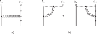
Figure 5: Diagrams for heavy quark anti-quark operator which are needed to show that the insertion of the operators (173) and (174) does not give a contribution.

In light cone gauge the only relevant diagram is always the exchange diagram and it vanishes for all two-particle operators, the only subtlety being, that since the operators are proportional to $\frac{1}{\xi}$ one has to take into account contractions of the gluon propagator with $n^{\mu}$ which are proportional to $\xi$:

$$n^{\mu}d_{\mu\nu}^{ab}(q,\xi) = -in^{\mu}\dfrac{\delta^{ab}}{q^{2}+i\epsilon}\left(g_{\mu\nu}-\dfrac{q_{\mu}n_{\nu}+q_{\nu}n_{\mu}}{n\cdot q}+q_{\mu}q_{\nu}\dfrac{n^{2}+\xi q^{2}}{(n\cdot q)^{2}}\right)$$ (175)

$$= -i\xi\dfrac{q_{\nu}}{n\cdot q}.$$

In covariant gauges the contributions from insertion of $\mathcal{O}_{v\cdot K}^{A}$ only vanish if one considers gauge invariant heavy-light light ray operators as in figure 5 b). This can be understood in the following way: Since in covariant gauges the $\log$- and integral-term in eq. (75) would have different colour structures the constraint (93) would be proportional to the difference of these. The insertion of $\mathcal{O}_{A}$ gives only a finite result as seen in (101) and therefore does not explain this result. Only the insertions of $\mathcal{O}_{v\cdot K}^{A}$ give the divergences with exactly the right colour structures to account for the changed commutator relation (93).

References

- (1) A. G. Grozin and M. Neubert, Phys. Rev. D 55 (1997) 272 [arXiv:hep-ph/9607366].
- (2) B. O. Lange and M. Neubert, Phys. Rev. Lett. 91 (2003) 102001 [arXiv:hep-ph/0303082].
- (3) V. M. Braun, D. Y. Ivanov and G. P. Korchemsky, Phys. Rev. D 69 (2004) 034014 [arXiv:hep-ph/0309330].
- (4) G. Bell and T. Feldmann, JHEP 0804 (2008) 061 [arXiv:0802.2221 [hep-ph]].
- (5) P. Ball, V. M. Braun and E. Gardi, Phys. Lett. B 665 (2008) 197 [arXiv:0804.2424 [hep-ph]].
- (6) S. Descotes-Genon and N. Offen, JHEP 0905 (2009) 091 [arXiv:0903.0790 [hep-ph]].
- (7) N. Offen and S. Descotes-Genon, PoS E FT09 (2009) 004 [arXiv:0904.4687 [hep-ph]].
- (8) H. Kawamura and K. Tanaka, Phys. Rev. D 81 (2010) 114009 [arXiv:1002.1177 [hep-ph]].
- (9) A. Khodjamirian, T. Mannel and N. Offen, Phys. Lett. B 620 (2005) 52 [arXiv:hep-ph/0504091].
- (10) A. Khodjamirian, T. Mannel and N. Offen, Phys. Rev. D 75 (2007) 054013 [arXiv:hep-ph/0611193].
- (11) S. J. Lee and M. Neubert, Phys. Rev. D 72 (2005) 094028 [arXiv:hep-ph/0509350].
- (12) H. Kawamura and K. Tanaka, Phys. Lett. B 673 (2009) 201 [arXiv:0810.5628 [hep-ph]].
- (13) A. G. Grozin and G. P. Korchemsky, Phys. Rev. D 53 (1996) 1378 [arXiv:hep-ph/9411323].
- (14) A. V. Efremov and A. V. Radyushkin, Phys. Lett. B 94 (1980) 245.
- (15) G. P. Lepage and S. J. Brodsky, Phys. Rev. D 22 (1980) 2157.
- (16) A. P. Bukhvostov, G. V. Frolov, L. N. Lipatov and E. A. Kuraev, Nucl. Phys. B 258 (1985) 601.
- (17) I. I. Balitsky and V. M. Braun, Nucl. Phys. B 311 (1989) 541.
- (18) V. M. Braun, A. N. Manashov and J. Rohrwild, Nucl. Phys. B 826 (2010) 235 [arXiv:0908.1684 [hep-ph]].
- (19) V. M. Braun, A. N. Manashov and J. Rohrwild, Nucl. Phys. B 807 (2009) 89 [arXiv:0806.2531 [hep-ph]].
- (20) V. M. Braun, G. P. Korchemsky and D. Mueller, Prog. Part. Nucl. Phys. 51 (2003) 311 [arXiv:hep-ph/0306057].
- (21) A. Bassetto, M. Dalbosco and R. Soldati, Phys. Rev. D 36 (1987) 3138.
- (22) S. L. Adler, J. C. Collins and A. Duncan, Phys. Rev. D 15 (1977) 1712.
- (23) J. C. Collins, A. Duncan and S. D. Joglekar, Phys. Rev. D 16 (1977) 438.
- (24) N. K. Nielsen, Nucl. Phys. B 120 (1977) 212.
- (25) P. Minkowski, “On The Anomalous Divergence Of The Dilatation Current In Gauge Theories,”
- (26) C. G. Callan, S. R. Coleman and R. Jackiw, Annals Phys. 59 (1970) 42.
- (27) A. V. Belitsky and D. Mueller, Nucl. Phys. B 527 (1998) 207 [arXiv:hep-ph/9802411].
- (28) A. V. Belitsky and D. Mueller, Nucl. Phys. B 537 (1999) 397 [arXiv:hep-ph/9804379].
- (29) S. E. Derkachov and A. N. Manashov, J. Math. Sci. 168 (2010) 837.
- (30) G. P. Korchemsky and A. V. Radyushkin, Nucl. Phys. B 283 (1987) 342.
- (31) S. Mandelstam, Nucl. Phys. B 213 (1983) 149.
- (32) G. Leibbrandt, Phys. Rev. D 29 (1984) 1699.
- (33) G. P. Korchemsky and A. V. Radyushkin, Phys. Lett. B 279 (1992) 359 [arXiv:hep-ph/9203222].
- (34) H. Kawamura, J. Kodaira, C. F. Qiao and K. Tanaka, Phys. Lett. B 523 (2001) 111 [Erratum-ibid. B 536 (2002) 344] [arXiv:hep-ph/0109181].
- (35) B. Geyer and O. Witzel, Phys. Rev. D 72 (2005) 034023 [arXiv:hep-ph/0502239].
- (36) B. Geyer and O. Witzel, Phys. Rev. D 76 (2007) 074022 [arXiv:0705.4357 [hep-ph]].