Fourier Transform Methods for Regime-Switching Jump-Diffusions and the Pricing of Forward Starting Options

Abstract

In this paper we consider a jump-diffusion dynamic whose parameters are driven by a continuous time and stationary Markov Chain on a finite state space as a model for the underlying of European contingent claims. For this class of processes we firstly outline the Fourier transform method both in log-price and log-strike to efficiently calculate the value of various types of options and as a concrete example of application, we present some numerical results within a two-state regime switching version of the Merton jump-diffusion model. Then we develop a closed-form solution to the problem of pricing a Forward Starting Option and use this result to approximate the value of such a derivative in a general stochastic volatility framework.

Key words: regime switching jump-diffusion models, option pricing, Fourier transform methods, Forward Starting Options, stochastic volatility models.

Mathematics Subject Classification (2010): 91G60, 91G20, 60J75.

1 Introduction

Since the paper by Naik (1993), the use of continuous time regime-switching processes to model asset price dynamics stimulated an increasing interest in the context of option pricing. The empirical evidence of a regime switching behavior of some economic time series was pointed out by Hamilton (1989, 1990), who suggested the use of an underlying Markov chain switching between regimes to account for some peculiarities in observed data. The ability of these econometric models to capture specific features such as volatility clustering and structural breaks is widely recognized (see e.g. Timmermann (2000)). Consequently, they can be considered as an appealing class of models also in the framework of derivative pricing. In the last decades there has been a considerable progress in the pricing exercise for plain vanilla European or American style options: see e.g. Di Masi et al. (1994), Bollen (1998), Guo (2001), Hardy (2001), Duan et al. (2002), Buffington and Elliott (2002), Konikov and Madan (2002), Guo and Zhang (2004), Chourdakis (2004,2007), Edwards (2005), Liu et al. (2006), Yao et al. (2006), Jobert and Rogers (2006), Elliott and Osakwe (2006), Jiang and Pistorius (2008), Boyarchenko and Levendorskii (2009), Khaliq and Liu (2009), Di Graziano and Rogers (2009), Ramponi (2009), Liu (2010). Comparatively few results are available for exotic options: see Boyle and Draviam (2007) and Elliott et al. (2007). Such results typically differ in the model considered (switching diffusions or more general Lévy processes), in the technique for solving the pricing problem (direct evaluation of expectations with respect to the probability density of the underlying, numerical solution of the associated PDE, recombining trees, Fourier transform methods) or in the type of financial product to price.

In this paper we consider a quite general underlying dynamic which can be seen as a switching L$\acute{\textrm{e}}$vy process of the I type, or finite activity L$\acute{\textrm{e}}$vy process (see e.g. Cont and Tankov (2004)). In particular, on a filtered probability space $(\Omega,\{\mathcal{F}_{t}\},\mathcal{F},\mathcal{P})$ the dynamic is of the form

$$S(t)=s_{0}\mathrm{e}^{X(t)}$$ (1)

where $X(t)$ is specified as a jump-diffusion whose parameters are driven by $\alpha(t)$, a continuous time and stationary Markov Chain on the state space $\mathcal{S}=\{1,2,\ldots,M\}$. This model provides an example of non-affine and non-Lévy process for which we are able to calculate the characteristic function (see Prop. 3.1) and therefore the pricing problem for European style options is efficiently faced through Fourier transform techniques. Such techniques, originated by the works of Heston (1993) and Carr and Madan (1999), are based on the representation of the value of the option in a proper Fourier space and have been successfully applied to a variety of pricing problems in the last years. Among the various contributions to this theory, see Bakshi and Madan (2000), Raible (2000), Lewis (2002), Lee (2004), Hubalek et al. (2006), Biagini et al. (2008), and more recently Cherubini et al. (2009), Dufresne et al. (2009), Hurd and Zhou (2010), Eberlein et al. (2010). Following this approach we can price various types of European options under the regime-switching dynamic by using the Fourier transform method both in the log-price space and in the log-strike space, consequently taking advantages from the powerful Fast Fourier Transform (FFT) computational tool. The case for a switching pure jump process has been considered in Elliott and Osakwe (2006).

As an application we consider the problem of valuing a Forward Starting option (FSO) for which an almost (i.e. up to numerical integration) closed-form solution is obtained in term of an integral transform. A similar technique was used in Kruse and Nögel (2005) to price a FSO in the Heston stochastic volatility model. These options are well-known exotic derivatives (see e.g. Hull (2009)) characterized by the payoff

$$\Pi_{T}(S(T),\kappa)=S(T)-\kappa S(t^{*})$$ (2)

where $t^{*}\in(0,T)$ is the determination time and $\kappa\in(0,1)$ is a given percentage. They are the building blocks of the so-called cliquet options. As it will be shown, our formula is very simple, being a finite mixture of call prices evaluated at the determination time under each regime, weighted by the stationary probability of the chain. Furthermore, in Chourdakis (2004) a procedure to approximate the value of an European option in a model with stochastic volatility and jumps was proposed by building a continuous-time Markov chain which ”mimics” the volatility process. The approximating dynamics turns out to be a regime-switching jump-diffusion model. By using such an approximation, a pricing algorithm for FSO in a general stochastic volatility model can be designed based on our mixture representation.

The paper is organized as follows. In Section 2 the dynamic model for the underlying is presented with a scheme for its numerical simulation and a useful representation through the sojourn times of the underlying Markov chain is introduced. In Section 3 the Fourier transform method both in log-price and log-strike is considered and formulas for the price of an European call option are explicitly derived. A numerical example of calibration on real data for a two-state regime switching jump diffusion model with gaussian jumps is reported. Finally, in Section 4 the price of a Forward starting option is obtained by using the Fourier transform representation and an algorithm to get approximate prices in a general stochastic volatility model is outlined.

2 The model

Let us consider on a filtered probability space $(\Omega,\{\mathcal{F}_{t}\},\mathcal{F},\mathcal{P})$, the asset price dynamic of the form

$$S(t)=s_{0}\mathrm{e}^{X(t)}$$ (3)

where $X(t)$ is specified as follows.

Let $\alpha(t)$ be a continuous time, homogeneous and stationary Markov Chain on the state space $\mathcal{S}=\{1,2,\ldots,M\}$ with a generator $Q\in\mathbb{R}^{M\times M}$; furthemore $\xi:\mathcal{S}\rightarrow\mathbb{R}$, $\sigma:\mathcal{S}\rightarrow\mathbb{R}$ and $\gamma:E\times\mathcal{S}\rightarrow\mathbb{R}$ are given functions, $(E,\mathcal{E})$ being a measurable mark space. In a given interval $0\leq t\leq T$, we consider the following dynamic

$$dX(t) = \xi(\alpha(t))dt+\sigma(\alpha(t))dW(t)+dJ(t),\ \ X(0)=0,$$

$$J(t) = \int_{0}^{t}\int_{E}\gamma(y,\alpha(s-))p^{\alpha}(dy,ds)$$

where $p^{\alpha}(dy,ds)$ is a marked point process (Runggaldier (2003)) characterized by the intensity

$$\lambda(\alpha,dy)=\lambda(\alpha)m(\alpha,dy).$$

Here $\lambda(\cdot)$ represents the (regime-switching) intensity of the Poisson process $N_{t}(E)$, while $m(\cdot,dy)$ are a set of probability measures on $(E,\mathcal{E})$, one for each state (regime) $i\in\mathcal{S}$ of the chain. The function $\gamma(y,\alpha)$ represents the jump amplitude relative to the mark $y$ in regime $\alpha$. Throughout the paper we assume that the processes $\alpha(\cdot)$ and $W(\cdot)$ are independent and that $W(\cdot)$ and $p^{\alpha}(dy,dt)$ are conditionally independent given $\alpha(t)$. We denote $\mathcal{F}^{\alpha}_{t}=\sigma\{\alpha(s):0\leq s\leq t\}$ the $\sigma$-algebra generated by the Markov chain. Furthermore, we assume that $\mathbf{E}[\mathrm{e}^{\gamma(Y(\alpha),\alpha)}]\equiv\int_{E}\mathrm{e}^{\gamma(y,\alpha)}m(\alpha,dy)$ is finite for each regime $\alpha$, where $Y(\alpha)$ is the random variable associated to the measure $m(\alpha,dy)$. We also define the compensated point process $q^{\alpha}(dy,dt)=p^{\alpha}(dy,dt)-\lambda(\alpha(t-))m(\alpha(t-),dy)dt$ in such a way

$$\int_{0}^{t}\int_{E}H(y,\alpha(s-))q^{\alpha}(dy,ds)$$

is a martingale in $t$ for each predictable process $H$ satisfying appropriate integrability conditions. In particular the jump process

$$J(t) = \int_{0}^{t}\int_{E}\gamma(y,\alpha(s-))q^{\alpha}(dy,ds)+\int_{0}^{t}\int_{E}\gamma(y,\alpha(s))\lambda(\alpha(s))m(\alpha(s),dy)ds$$

$$= \tilde{J}(t)+\int_{0}^{t}\lambda(\alpha(s))\mathbf{E}[\gamma(Y(\alpha(s)),\alpha(s))]ds,\ \ \ Y(\alpha(s))\sim m(\alpha(s),dy)$$

is the sum of a martingale and an absolutely continuous process, whenever $\gamma$ satisfies the proper conditions.

A sample path of this process is generated as follows (see Fig.1):

1. generate a path of the Markov chain, i.e. a set of switching times $\tau_{0}=0,\tau_{1},\ldots,\tau_{L},\tau_{L+1}=T$ and the corresponding states $\alpha(t)=\alpha_{k}\in\mathcal{S},\tau_{k}\leq t<\tau_{k+1},k=0,\ldots,L$;

2. generate the jump times $\upsilon_{k_{j}}$ of the Poisson process in each interval $[\tau_{k},\tau_{k+1})$ according to the intensity $\lambda(\alpha_{k})$ and let $N_{k}$ be the number of jumps;

3. for any $k=0,\ldots,L$ generate $N_{k}$ i.i.d. samples $Y(\alpha(\upsilon_{k_{j}})),j=1,\ldots,N_{k}$ distributed according to the probability $m(\alpha_{k},dy)$;

4. on a given time grid $t_{0},\ldots,t_{n}$ of $[0,T]$ built as the superposition of a deterministic grid and the jump times $\upsilon_{j}$, let $X(t_{0})=0$ and

   $$X(t_{i+1}-) = X(t_{i})+\xi(\alpha(t_{i}))(t_{i+1}-t_{i})+\sigma(\alpha(t_{i}))(W(t_{i+1}-W(t_{i})),$$ (4)

   $$X(t_{i+1}) = X(t_{i+1}-)+\int_{E}\gamma(y,\alpha(t_{i+1}))p(dy,t_{i+1}).$$ (5)

   If $t_{i+1}$ is actually a point of the Poisson random measure, the magnitude of the jump is sampled, that is

   $$\int_{E}\gamma(y,\alpha(t_{i+1})p(dy,t_{i+1})=\gamma(Y(\alpha(t_{i+1})),\alpha(t_{i+1})),$$

   otherwise the jump term is zero.

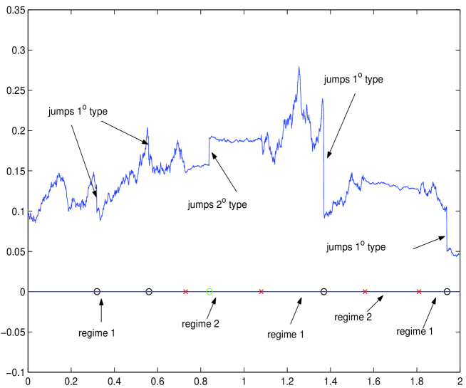
Figure 1: A sample path of the RSJD - Example 2.1. Red cross are the switching times, circles represent the jump times for the two regimes.

In view of our pricing application, from now on we assume to specify our model in a probability space where the ”discounted” asset price $\tilde{S}(t)=S(t)\mathrm{e}^{-\int_{0}^{t}\mu(\alpha(s))ds}$ is a martingale. In particular, we keep the function $\mu:\mathcal{S}\rightarrow\mathbb{R}$ unspecified in order to cope with slightly different types of contracts: for example, given the risk-free rate $r$, we can set $\mu(\alpha)=\mu$ with $\mu=r-q$, $q$ being the (continuous) dividend rate, $\mu=r-r_{f}$, $r_{f}$ being the foreign risk-free rate or more generally $\mu(\alpha)=r(\alpha)-q(\alpha)$ if rates and dividend are regime-switching too.

We therefore consider the following model

$$X(t) = \int_{0}^{t}\left(\mu(\alpha(s))-\frac{1}{2}\sigma^{2}(\alpha(s))-\lambda(\alpha(s))\kappa(\alpha(s))\right)ds+\int_{0}^{t}\sigma(\alpha(s))dW(s)$$ (6)

$$+ \int_{0}^{t}\int_{E}\gamma(y,\alpha(s^{-}))p^{\alpha}(dy,ds),$$

where

$$\kappa(\alpha)=\mathbf{E}[(\mathrm{e}^{\gamma(Y(\alpha),\alpha)}-1)],\ \ \alpha\in\mathcal{S}.$$

An application of the generalized Ito’s Formula gives

$$d\tilde{S}(t) = \tilde{S}(t-)\left(-\lambda(\alpha(t))\kappa(\alpha(t))dt+\sigma(\alpha(t))dW(t)+\int_{E}(\mathrm{e}^{\gamma(y,\alpha(t-))}-1)p^{\alpha}(dy,dt)\right)$$

$$= \tilde{S}(t-)\left(\sigma(\alpha(t))dW(t)+\int_{E}(\mathrm{e}^{\gamma(y,\alpha(t-))}-1)q^{\alpha}(dy,dt)\right),$$

where $q^{\alpha}(dy,dt)=p^{\alpha}(dy,dt)-\lambda(\alpha(t-))\kappa(\alpha(t-))dt$ is the compensated process. Hence, $\tilde{S}(t)$ is a martingale. The corresponding jump-diffusion SDE for the asset price is therefore

$$\frac{dS(t)}{S(t-)}=(\mu(\alpha(t))-\lambda(\alpha(t))\kappa(\alpha(t)))dt+\sigma(\alpha(t))dW(t)+\int_{E}(\mathrm{e}^{\gamma(y,\alpha(t-))}-1)p^{\alpha}(dy,dt),\ \ \ S(0)=s_{0}.$$ (7)

Example 2.1

As a working example we consider a two-state regime switching version of the Merton jump-diffusion model. This is defined by taking $\gamma(y,\alpha)=y$ and two kinds of normal jumps, i.e. $Y(i)\sim\mathcal{N}(a_{i},b_{i})$ from which $\kappa(i)=\mathbf{E}[(\mathrm{e}^{Y(i)}-1)]=\mathrm{e}^{a_{i}+b_{i}^{2}/2}-1$, $i=1,2$. The two state Markov chain $\alpha(t)\in\mathcal{S}=\{1,2\}$ has generator $Q=\left(\begin{array}[]{cc}-q_{1}&q_{1}\\ q_{2}&-q_{2}\\ \end{array}\right)$. Let $\sigma_{i},\lambda_{i}>0$ and $\mu_{i},i=1,2$ be given parameters: the regime switching jump-diffusion Merton model is defined as

$$dX(t) = [\mu(\alpha(t))-\frac{1}{2}\sigma^{2}(\alpha(t)-\lambda(\alpha(t))\kappa(\alpha(t))]dt+\sigma(\alpha(t))dW(t)+dJ(t)$$

$$J(t) = \int_{0}^{t}\int_{E}yp^{\alpha}(dy,ds),\ \ \ \lambda(t,\alpha(t),dy)=\lambda(\alpha(t))\phi_{\alpha(t)}(y)dy$$

where $\lambda(\alpha(t))\in\{\lambda_{1},\lambda_{2}\}$, $\sigma(\alpha(t))\in\{\sigma_{1},\sigma_{2}\}$, $\mu(\alpha(t))\in\{\mu_{1},\mu_{2}\}$ and $\lambda(t,\alpha(t),dy)$ is the intensity process of the Poisson jump component, $\phi_{i}(y)$ being the density of a normal distribution $\mathcal{N}(a_{i},b_{i})$, $i=1,2$. $\Box$

Next Proposition gives a useful representation for $X(T)$. A sketch of the proof is reported in the Appendix.

Proposition 2.1

Let $T_{i}=\int_{0}^{T}\mathbb{I}_{\alpha(s)=i}ds$, $i=1,\ldots,M$ be the occupation times of the Markov chain and let us define $\xi(\alpha)=\mu(\alpha)-\frac{1}{2}\sigma^{2}(\alpha)-\lambda(\alpha)\kappa(\alpha)$ and

$$\Xi_{T}(T_{1},\ldots,T_{M})=\int_{0}^{T}\xi(\alpha(s))ds=\sum_{i=1}^{M}\xi(i)T_{i}.$$

Then the process $X(T)$ admits the following representation:

$$X(T)=\Xi_{T}(T_{1},\ldots,T_{m})+\sum_{i=1}^{M}\sigma(i)Z(\Delta_{i})+\sum_{i=1}^{M}\sum_{k=1}^{N(\Delta_{i})}Y^{(i)}_{k},$$ (8)

where $N(\Delta_{i})$ and $Z(\Delta_{i})$ are distributed as Poisson variables $\mathrm{Poiss}(\lambda_{i}T_{i})$ and as Normal variables $\mathcal{N}(0,T_{i})$, respectively, $i=1,\ldots,M$.

It is readly seen that by defining $X_{t,T}=X(T)-X(t)$ we have

$$X_{t,T}=\Xi_{t,T}(T^{t,T}_{1},\ldots,T^{t,T}_{M})+\sum_{i=1}^{M}\sigma(i)Z(\Delta_{i})+\sum_{i=1}^{M}\sum_{k=1}^{N(\Delta_{i})}Y^{(i)}_{k},$$ (9)

where $T^{t,T}_{j}=\int_{t}^{T}\mathbb{I}_{\alpha(s)=j}ds$, $j=1,\ldots,M$, and the random variables $N(\Delta_{i})$ and $Z(\Delta_{i})$ have conditional distributions $\mathrm{Poiss}(\lambda_{i}(T_{i}-t))$ and $\mathcal{N}(0,T_{i}-t)$. Correspondingly we can write $S(T)=S(t)\exp(X_{t,T})$.

Remark 2.1

Notice that for a L$\acute{\textrm{e}}$vy process $X_{L}(t)$ having characteristic function

$$\mathbf{E}[\mathrm{e}^{\mathrm{i}uX_{L}(t)}]=\exp\left(t(\mathrm{i}\xi u-\frac{\sigma^{2}u^{2}}{2}+\int_{\mathbb{R}}(e^{\mathrm{i}ux}-1)\beta(dx))\right)$$

the expected value is $\mathbf{E}[X_{L}(T)]=T(\xi+\int_{\mathbb{R}}x\beta(dx))$. For our RS model, it follows from (2.1) that

$$\mathbf{E}[X(T)]=\sum_{i=1}^{m}(\xi(i)+\lambda(i)\mu_{Y^{(i)}})\mathbf{E}[T_{i}]=\sum_{i=1}^{m}(\xi(i)+\lambda(i)\mu_{Y^{(i)}})\int_{0}^{T}\mathcal{P}(\alpha(s)=i|\alpha(0))ds.$$

This quantity can be easily evaluated for a two-state MC, since we have $P_{s}=\mathrm{e}^{Qs}=\frac{1}{\mu+\nu}\left(\begin{array}[]{cc}\mu\mathrm{e}^{-s(\mu+\nu)}+\nu&\mu(1-\mathrm{e}^{-s(\mu+\nu)})\\ \nu(1-\mathrm{e}^{-s(\mu+\nu)})&\nu\mathrm{e}^{-s(\mu+\nu)}+\mu\\ \end{array}\right)$. This implies that, starting e.g. from $\alpha(0)=1$

$$\mathbf{E}[X(T)] = (\xi(1)+\lambda(1)\mu_{Y^{(1)}})(\frac{\mu}{\mu+\nu}\frac{1-\mathrm{e}^{-T(\mu+\nu)}}{\mu+\nu}+\frac{\nu}{\mu+\nu}T)$$

$$+ (\xi(2)+\lambda(2)\mu_{Y^{(2)}})(-\frac{\mu}{\mu+\nu}\frac{1-\mathrm{e}^{-T(\mu+\nu)}}{\mu+\nu}+\frac{\mu}{\mu+\nu}T).$$

3 The transform method

Our main interest is the efficient numerical evaluation of the price $\Pi_{0}$ of an European contingent claim specified by the payoff function $\Pi(s,K)$, exercised at the future time $T$, $K$ being a trigger parameter. By letting $r(t)$ be the interest rate process, $B(t)=\exp(\int_{0}^{t}r(u)du)$ the usual money market account and $P(t,T)$ the time-$t$ value of a discount bond maturing at $T$, arbitrage pricing theory and a change-of-numeraire technique give the well-known characterization of prices

$$\Pi_{0}=\mathbf{E}^{\mathcal{P}}[B(T)^{-1}\Pi(S(T),K)]=P(0,T)\mathbf{E}^{\mathcal{Q}}[\Pi(S(T),K)],\ \ \ P(0,T)=\mathbf{E}^{\mathcal{P}}[B(T)^{-1}],$$

where $\mathcal{P}$ is the risk-neutral measure and $\mathcal{Q}$ is known as $T$-forward measure. When interest rates are deterministic, the two measures are equal. In the following we assume that our dynamic model is given under the measure $\mathcal{Q}$. All the expected values will be considered with respect to this measure.

It is well known that Fourier transform methods can be efficiently used for the valuation of European style options. Two main variants have been developed depending on which variable of the payoff is transformed into the Fourier space. In view of the structure assumed for the dynamic of the underlying price $S(T)$ and our next applications, we consider instead $\log(S(T))=X(T)+\log(s_{0})$ as the state variable and $k=\log(K)$ for the trigger parameter, in such a way for any payoff $\Pi(s,K)=\Pi(e^{\log(s)},e^{\log(K)})\equiv\Pi(y,k)$. Correspondingly, we can consider the generalized Fourier transform with respect to the state variable $y$, $\hat{\Pi}_{k}(z)=\int_{\mathbb{R}}\mathrm{e}^{\mathrm{i}zy}\Pi(y,k)dy$ (log-price transform), or w.r.t. the trigger $k$, $\hat{\Pi}_{y}(z)=\int_{\mathbb{R}}\mathrm{e}^{\mathrm{i}zk}\Pi(y,k)dk$ (log-strike transform), $z\in\mathbb{C}$. In general we assume that these transforms exist in some strip $\mathcal{S}_{\Pi}=\{z\in\mathbb{C}:-\infty\leq a<\Im(z)<b\leq+\infty\}$ of the complex plane. Examples of payoffs are reported in Table (1). The first approach was proposed in this form in Raible (2000) (but the representation of option prices through inversion of characteristic function appeared for the first time in Heston (1993)), while the second was introduced in Carr and Madan (1999).

Formally, Fourier inversion gives

$$\Pi(y,k)=\left\{\begin{array}[]{cc}\frac{1}{2\pi}\int_{\mathrm{i}\nu-\infty}^{\mathrm{i}\nu+\infty}\mathrm{e}^{-\mathrm{i}zy}\hat{\Pi}_{k}(z)dz,&\mbox{log-price transform}\\ \\ \frac{1}{2\pi}\int_{\mathrm{i}\nu-\infty}^{\mathrm{i}\nu+\infty}\mathrm{e}^{-\mathrm{i}zk}\hat{\Pi}_{y}(z)dz,&\mbox{log-strike transform}\\ \end{array}\right.$$

where integrals are considered along the straight line $\Im(z)=\nu$ in the complex plane. By letting $\varphi_{T}(z)=\mathbf{E}[\mathrm{e}^{\mathrm{i}zX(T)}],\ z\in\mathbb{C}$ be the (generalized) Fourier transform (or characteristic function) of $X(T)$, we have

$$\Pi_{0}/P(0,T)=\mathbf{E}^{\mathcal{Q}}[\Pi(X(T)+\log(s_{0}),k)]=\int_{\mathbb{R}}\Pi(y,k)\mathcal{Q}_{T}(dy)$$

$$=\left\{\begin{array}[]{c}\int_{\mathbb{R}}\frac{1}{2\pi}\int_{\mathrm{i}\nu-\infty}^{\mathrm{i}\nu+\infty}\mathrm{e}^{-\mathrm{i}zy}\hat{\Pi}_{k}(z)dz\mathcal{Q}_{T}(dy)\\ \\ \int_{\mathbb{R}}\frac{1}{2\pi}\int_{\mathrm{i}\nu-\infty}^{\mathrm{i}\nu+\infty}\mathrm{e}^{-\mathrm{i}zk}\hat{\Pi}_{y}(z)dz\mathcal{Q}_{T}(dy)\\ \end{array}\right.=\left\{\begin{array}[]{c}\frac{1}{2\pi}\int_{\mathrm{i}\nu-\infty}^{\mathrm{i}\nu+\infty}\hat{\Pi}_{k}(z)\int_{\mathbb{R}}\mathrm{e}^{-\mathrm{i}zy}\mathcal{Q}_{T}(dy)dz\\ \\ \frac{1}{2\pi}\int_{\mathrm{i}\nu-\infty}^{\mathrm{i}\nu+\infty}\mathrm{e}^{-\mathrm{i}zk}\int_{\mathbb{R}}\hat{\Pi}_{y}(z)\mathcal{Q}_{T}(dy)dz\\ \end{array}\right.$$

$$=\left\{\begin{array}[]{ll}\frac{1}{2\pi}\int_{\mathrm{i}\nu-\infty}^{\mathrm{i}\nu+\infty}\mathrm{e}^{-\mathrm{i}z\log(s_{0})}\hat{\Pi}_{k}(z)\varphi_{T}(-z)dz,&\mbox{log-price transform}\\ \\ \frac{1}{2\pi}\int_{\mathrm{i}\nu-\infty}^{\mathrm{i}\nu+\infty}\mathrm{e}^{-\mathrm{i}zk}\mathbf{E}^{\mathcal{Q}}[\hat{\Pi}_{X(T)+\log(s_{0})}(z)]dz,&\mbox{log-strike transform}.\\ \end{array}\right.$$ (10)

In order to justify the previous equalities, some conditions are required: existence of the generalized Fourier transform $\hat{\Pi}$, integrability along the contour $\Im(z)=\nu$ in some strip $\mathcal{S}_{\Pi}$ in order to guarantee the Inversion Theorem and existence of the expectation $\mathbf{E}^{\mathcal{Q}}[e^{\nu X(T)}]$ (see Lee (2004) for log-strike transform, Lewis (2002) or the recent Eberlein et al. (2009) for log-price transform). Notice that the use of generalized Fourier transform permits to exploit contour variations by means of the residue theorem, as it will be seen in next paragraphs.

Due to the exponential structure of the GFT of typical payoffs (see Table (1)), also for the log-strike transform it is required the calculation of $\varphi_{T}(z)$ appearing through the expectation $\mathbf{E}^{\mathcal{Q}}[\hat{\Pi}_{X(T)+\log(s_{0})}(z)]$. Next Proposition gives the GFT of our process. Similar results are available (see Chourdakis (2004)) where a particular structure of the generator $Q$ is considered: for completeness, we report the proof in the Appendix.

Payoff	GFT in log-price	Strip of regularity	GFT in log-strike	Strip of regularity
$(\mathrm{e}^{y}-\mathrm{e}^{k})^{+}$	$\frac{\mathrm{e}^{k(\mathrm{i}z+1)}}{\mathrm{i}z-z^{2}}$	$\Im(z)>1$	$\frac{\mathrm{e}^{y(\mathrm{i}z+1)}}{\mathrm{i}z-z^{2}}$	$\Im(z)<0$
$(\mathrm{e}^{k}-\mathrm{e}^{y})^{+}$	$\frac{\mathrm{e}^{k(\mathrm{i}z+1)}}{\mathrm{i}z-z^{2}}$	$\Im(z)<0$	$\frac{\mathrm{e}^{y(\mathrm{i}z+1)}}{\mathrm{i}z-z^{2}}$	$\Im(z)>1$
$\mathrm{e}^{ay}\mathbb{I}_{by>\kappa}$	$-\frac{\mathrm{e}^{(a+\mathrm{i}z)\kappa/b}}{a+\mathrm{i}z}$	$\Im(z)>a$	$\frac{\mathrm{e}^{(a+\mathrm{i}zb)y}}{\mathrm{i}z}$	$\Im(z)>0$
$\min(\mathrm{e}^{y},\mathrm{e}^{k})$	$\frac{\mathrm{e}^{k(\mathrm{i}z+1)}}{z^{2}-\mathrm{i}z}$	$0<\Im(z)<1$	$\frac{\mathrm{e}^{y(\mathrm{i}z+1)}}{z^{2}-\mathrm{i}z}$	$0<\Im(z)<1$

Table 1: Generalized Fourier transforms of typical payoffs.

Proposition 3.1

Let $\phi_{j}(z)=\mathbf{E}[\mathrm{e}^{\mathrm{i}z\gamma(Y(j),j)}]$ be the generalized Fourier transform of the jump magnitude. Then, by letting

$$\vartheta_{j}(z)=z\xi(j)+\frac{1}{2}\mathrm{i}z^{2}\sigma^{2}(j)-\mathrm{i}\lambda(j)(\phi_{i}(z)-1)$$ (11)

and $\tilde{\vartheta}_{i}(z)=\vartheta_{j}(z)-\vartheta_{M}(z)$, we have

$$\begin{array}[]{lll}\varphi_{T}(z)&=&\mathrm{e}^{\mathrm{i}\vartheta_{M}(z)T}\left(\mathbf{1}^{\prime}\cdot\mathrm{e}^{(Q^{\prime}+\mathrm{i}\ \mathrm{diag}(\tilde{\vartheta}_{1}(z),\ldots,\tilde{\vartheta}_{M-1}(z),0))T}\cdot\mathbb{I}(0)\right)\\ \\ &=&\mathbf{1}^{\prime}\cdot\mathrm{e}^{(Q^{\prime}+\mathrm{i}\ \mathrm{diag}(\vartheta_{1}(z),\ldots,\vartheta_{M}(z)))T}\cdot\mathbb{I}(0),\end{array}$$ (12)

where $\mathbf{1}=(1,\ldots,1)^{\prime}\in\mathbb{R}^{M\times 1}$, $\mathbb{I}(0)=(\mathbb{I}_{\alpha(0)=1},\ldots,\mathbb{I}_{\alpha(0)=M})^{\prime}\in\mathbb{R}^{M\times 1}$ and $Q^{\prime}$ is the transpose of $Q$.

Remark 3.1

Notice that $\varphi_{T}(0)=1$ and $\varphi_{T}(-\mathrm{i})=\mathbf{E}\left[\mathrm{e}^{\sum_{j=1}^{M}\mu(j)T_{j}}\right]$. Furthermore, if $\mu(\alpha)\equiv\mu$, then $\varphi_{T}(-\mathrm{i})=\mathrm{e}^{\mu T}$ since $\sum_{i=1}^{m}T_{i}=T$.

More generally, we get from (9) and (12)

$$\begin{array}[]{lll}\varphi_{t,T}(z)&=&\mathbf{E}_{t}[\mathrm{e}^{\mathrm{i}zX_{t,T}}]=\left(\mathbf{1}^{\prime}\cdot\mathrm{e}^{(Q^{\prime}+\mathrm{i}\ \mathrm{diag}(\vartheta_{1}(z),\ldots,\vartheta_{M}(z)))(T-t)}\cdot\mathbb{I}(t)\right)\\ \\ &=&\sum_{j=1}^{M}\mathbb{I}_{\alpha(t)=j}\mathrm{q}_{j}^{t,T}(z),\ \ \ \ \ \mathrm{q}_{j}^{t,T}(z)=\sum_{k=1}^{M}\left(\mathrm{e}^{(Q^{\prime}+\mathrm{i}\ \mathrm{diag}(\vartheta_{1}(z),\ldots,\vartheta_{M}(z)))(T-t)}\right)_{kj},\end{array}$$ (13)

for any $t\in[0,T)$, $\mathbf{E}_{t}$ being the conditional expectation up to time $t$. Notice that the characteristic function of $X(T)$ and $X_{t,T}$ depends on the state of the Markov chain $\alpha(0)$ and $\alpha(t)$, respectively.

The conditions for applying the transform method both in log-price and log-strike depend on the properties of the GTF of $X(T)$, which in turn depend on that of $\phi_{j}(z)$ through Proposition 3.1. In general, these functions are well defined (and analytic) in some strips of the complex plane

$$\mathcal{S}_{j}=\{z\in\mathbb{C}:\mathbf{E}^{\mathcal{Q}}[e^{\Im(z)\gamma(Y(j),j)}]<\infty\},\ \ j=1,\ldots,M.$$

Let us define the matrix $A(z)=Q^{\prime}+\mathrm{i}\ \mathrm{diag}(\vartheta_{1}(z),\ldots,\vartheta_{M}(z))$: clearly the elements of $A(z)^{n},n=1,2,\ldots$ are polynomials in the $\vartheta_{j}(z)$’s and therefore these are well defined in the intersection of the $\mathcal{S}_{j}$, $j=1,\dots,M$. From the properties of the matrix exponential function $e^{A(z)}=\sum_{n=1}^{+\infty}\frac{A(z)^{n}}{n!}$ and since the GTF of $X(T)$ is a linear combination of its elements, it immediately follows that (12) and (13) are well defined in $\bigcap_{j=1}^{M}\mathcal{S}_{j}$ and consequently the transform methods can be applied, provided $\bigcap_{j=1}^{M}\mathcal{S}_{j}\neq\emptyset$ and the payoffs satisfy the proper conditions.

Remark 3.2

If we set $\mu(i)=\mu,\sigma(i)=\sigma$, $\lambda(i)=\lambda$ and $\phi_{i}(z)=\phi(z)$ we have that $\tilde{\vartheta}_{i}(z)=0$, $i=1,\ldots,m-1$, and the term $\exp(Q^{\prime}T)$ is the transpose of the transition semi-group of the Markov chain. Under these choices we are implicitly assuming a unique regime and eq. (13) becomes the well-known characteristic function of the (single-regime) jump-diffusion dynamic (6), $\varphi_{T}(z)=\exp(z\xi+\frac{1}{2}\mathrm{i}z^{2}\sigma^{2}-\mathrm{i}\lambda(\phi(z)-1))$. This is because $\mathbf{1}^{\prime}\cdot\mathrm{e}^{(Q^{\prime}+\mathrm{i}\ \mathrm{diag}(\tilde{\vartheta}_{1}(z),\ldots,\tilde{\vartheta}_{M-1}(z),0))(T-t)}\cdot\mathbb{I}(t)=\mathbf{1}^{\prime}\cdot\mathrm{e}^{Q^{\prime}(T-t)}\cdot\mathbb{I}(t)=\sum_{i=1}^{M}\mathbb{I}_{\alpha(t)=i}=1$. Hence, with simple linear constraints on the full parameter set of our dynamic (6) we can recover several models:

1. Black & Scholes model (BS): $\mu_{i}=r$, $\sigma_{i}=\sigma>0$, $\lambda_{i}=0$ (we consequently set to zero the jump variables $Y(i)$), $i=1,\ldots,M$;

2. Black & Scholes with regime switching model (RSBS): $\mu_{i}\in\mathbb{R}$, $\sigma_{i}>0$, $q_{ij}>0,i\neq j$, $\lambda_{i}=0$ ($Y(i)\equiv 0$), $i=1,\ldots,M$;

3. Merton jump-diffusion model (JDM): $\mu_{i}=r$, $\sigma_{i}=\sigma>0$, $\lambda_{i}=\lambda>0$ and the parameters of the jump variables $Y_{i}\equiv Y$, $i=1,\ldots,M$;

4. Merton jump-diffusion model with regime switching (RSJDM): $\mu_{i}\in\mathbb{R}$, $\sigma_{i}>0$, $q_{ij}>0,i\neq j$, $\lambda_{i}>0$ and the parameters of the jump variables $Y(i)$ for each regime, $i=1,\ldots,M$.

From a computational viewpoint, for a fixed complex $z$ the calculation of $\varphi_{T}(z)$ requires the following steps:

1. calculate $\vartheta_{j}(z),j=1,\ldots,M$ (eq. (11));

2. form the matrix $A(z)=Q^{\prime}+\mathrm{i}\ \mathrm{diag}(\vartheta_{1}(z),\ldots,\vartheta_{M}(z))$;

3. calculate the matrix exponential $\Phi(z)=\exp(A(z)\ T)$;

4. for each starting state of the chain $\alpha(0)=j,j=1,\ldots,M$, calculate $\mathrm{q}_{j}^{T}(z)=\sum_{k=1}^{M}\Phi_{kj}(z)$.

For $M>2$ the cumbersome task is the calculation of $\Phi$ for which efficient numerical techniques are available (see Higham (2009)).

The case M=2.

In this case it is possible to give a closed form solution to the matrix exponential, therefore obtaining an easy-to-implement formula for the characteristic function. The following result can be proved either by solving a couple of ODE, as in Buffington and Elliott (2002) - Appendix 1, or through a Laplace Transform - based technique, as in Liu et al. (2006).

Proposition 3.2

Let $y_{1,2}$ be the solutions of the quadratic equation $y^{2}+(q_{1}+q_{2}-\mathrm{i}\theta)y-\mathrm{i}\theta q_{2}=0$ and

$$\begin{array}[]{lll}\mathrm{q}_{1}^{t,T}(\theta)&=&\frac{1}{y_{1}-y_{2}}\left(\mathrm{e}^{y_{1}(T-t)}(y_{1}+q_{1}+q_{2})-\mathrm{e}^{y_{2}(T-t)}(y_{2}+q_{1}+q_{2})\right)\\ \\ \mathrm{q}_{2}^{t,T}(\theta)&=&\frac{1}{y_{1}-y_{2}}\left(\mathrm{e}^{y_{1}(T-t)}(y_{1}+q_{1}+q_{2}-\mathrm{i}\theta)-\mathrm{e}^{y_{2}(T-t)}(y_{2}+q_{1}+q_{2}-\mathrm{i}\theta)\right).\end{array}$$

Then

$$\mathbf{E}_{t}[\mathrm{e}^{\mathrm{i}\theta T_{1}}]=\mathbb{I}_{\alpha(t)=1}\mathrm{q}_{1}^{t,T}(\theta)+\mathbb{I}_{\alpha(t)=2}\mathrm{q}_{2}^{t,T}(\theta).$$

$\Box$

It is easy to prove that the functions $\mathrm{q}_{1}^{t,T}$ and $\mathrm{q}_{2}^{t,T}$ are invariant by changing the order of the roots $y_{1}$ and $y_{2}$. The characteristic function follows from the proof of Prop. 3.1 (see (32)):

$$\varphi_{t,T}(z)=\mathrm{e}^{\mathrm{i}\vartheta_{2}(z)(T-t)}\left(\mathbb{I}_{\alpha(t)=1}\mathrm{q}_{1}^{t,T}(\theta(z))+\mathbb{I}_{\alpha(t)=2}\mathrm{q}_{2}^{t,T}(\theta(z))\right).$$ (14)

Example 3.1

In our regime switching version of the Merton model we have $\phi_{i}(z)=\mathrm{e}^{\mathrm{i}za_{i}-\frac{1}{2}z^{2}b^{2}_{i}}$, $i=1,\ldots,M.$ Then, from (11)

$$\vartheta_{i}(z)=z\xi_{i}+\frac{1}{2}\mathrm{i}z^{2}\sigma^{2}_{i}-\mathrm{i}\lambda_{i}(\mathrm{e}^{\mathrm{i}za_{i}-\frac{1}{2}z^{2}b^{2}_{i}}-1),\ \ i=1,\ldots,M.$$ (15)

It follows that in such a case the characteristic function $\varphi_{T}(z)$ is well defined for all $z\in\mathbb{C}$. In the two state model the GFT is easily obtained from (14).

Some examples of payoff transforms for the typical claims are recalled in Table 1. In view of our next applications, we show in some details how to get the price of call and put options both in log-price and in log-strike transform. Pricing formulas for the other payoffs are reported in Table 2.

Call/Put value in $\log$-price transform.

From formula (10) and Table 1 we get for the call option

$$C_{0}=\frac{P(0,T)}{2\pi}\int_{\mathrm{i}\nu-\infty}^{\mathrm{i}\nu+\infty}\mathrm{e}^{-\mathrm{i}z\log(s_{0})}\varphi_{T}(-z)\frac{\mathrm{e}^{k(\mathrm{i}z+1)}}{\mathrm{i}z-z^{2}}dz,\ \ \nu>1,$$ (16)

$$=\frac{P(0,T)}{2\pi}\ \mathrm{e}^{\nu\log(s_{0})+k(1-\nu)}\int_{-\infty}^{+\infty}\mathrm{e}^{-\mathrm{i}u(\log(s_{0})-k)}\frac{\varphi_{T}(-u-\mathrm{i}\nu)}{\nu^{2}-\nu-u^{2}+\mathrm{i}u(1-2\nu)}du$$

$$=\frac{P(0,T)}{2\pi}\ s_{0}^{\nu}K^{1-\nu}\int_{-\infty}^{+\infty}\mathrm{e}^{-\mathrm{i}u\log(s_{0}/K)}\frac{\varphi_{T}(-u-\mathrm{i}\nu)}{\nu^{2}-\nu-u^{2}+\mathrm{i}u(1-2\nu)}du,$$

provided the characteristic function evaluated in the integral (16) is well defined for $z\in\mathbb{C}$ such that $\Im(z)>1$. By switching from $\Im(z)>1$ to $\Im(z)<0$ we get the value for the put option: notice that the put-call parity relation is recovered by moving the integration contour. As a matter of fact, alternative formulas can be derived by using residue calculus (see e.g. Lewis(2002)), under the proper conditions for $\varphi_{T}(z)$. The GFT of this payoff has two simple poles at $z=0$ and $z=\mathrm{i}$ with residue $-\frac{K\mathrm{i}}{2\pi}$ and $\frac{s_{0}\varphi_{T}(-\mathrm{i})\mathrm{i}}{2\pi}$, respectively: by moving the integration contour and since the integral must be real, we obtain the following general formula in which we stress the dependence on $s_{0}$, $\alpha_{0}$ and $K$:

$$C_{0}(s_{0},\alpha_{0},K)=P(0,T)\left(R_{\nu}+\frac{1}{2\pi}\int_{\mathrm{i}\nu-\infty}^{\mathrm{i}\nu+\infty}\mathrm{e}^{-\mathrm{i}z\log(s_{0})}\varphi_{T}(-z)\frac{\mathrm{e}^{k(\mathrm{i}z+1)}}{\mathrm{i}z-z^{2}}dz\right)$$ (17)

$$=P(0,T)\left(R_{\nu}+\frac{1}{\pi}s_{0}^{\nu}K^{1-\nu}\int_{0}^{+\infty}\Re\left[\mathrm{e}^{-\mathrm{i}u\log(s_{0}/K)}\frac{\varphi_{T}(-u-\mathrm{i}\nu)}{\nu^{2}-\nu-u^{2}+\mathrm{i}u(1-2\nu)}\right]du\right)$$

$$=P(0,T)\left(R_{\nu}+\frac{1}{\pi}s_{0}^{\nu}K^{1-\nu}\sum_{j=1}^{M}\mathbb{I}_{\alpha(0)=j}\int_{0}^{+\infty}\Re\left[\frac{\mathrm{e}^{-\mathrm{i}u\log(s_{0}/K)}\mathrm{q}_{j}^{0,T}(-u-\mathrm{i}\nu)}{\nu^{2}-\nu-u^{2}+\mathrm{i}u(1-2\nu)}\right]du\right),$$ (18)

$$R_{\nu}=\left\{\begin{array}[]{ll}0&\nu>1\\ s_{0}\frac{\varphi_{T}(-\mathrm{i})}{2}&\nu=1\\ s_{0}\varphi_{T}(-\mathrm{i})&0<\nu<1\\ s_{0}\varphi_{T}(-\mathrm{i})-\frac{\mathrm{e}^{k}}{2}&\nu=0\\ s_{0}\varphi_{T}(-\mathrm{i})-\mathrm{e}^{k}&\nu<0\\ \end{array}\right.$$

where $\varphi_{T}(-\mathrm{i})=\mathbf{E}[\mathrm{e}^{\sum_{i=1}^{m}\mu_{i}T_{i}}]$ according to Remark (3.1) and the functions $\mathrm{q}_{i}^{0,T}(\cdot)$ are defined in (13).

Call/Put value in $\log$-strike transform.

As before, if the GFT $\phi_{j}(\cdot)$ are well defined functions in a properly defined strip of $\mathbb{C}$, from formula (10) and Table 1, we get for the call option

$$\mathbf{E}^{\mathcal{Q}}[\hat{\Pi}_{X(T)+\log(s_{0})}(z)]=\frac{\mathbf{E}[\mathrm{e}^{(X(T)+\log(s_{0}))(\mathrm{i}z+1)}]}{\mathrm{i}z-z^{2}}=\frac{\mathrm{e}^{\log(s_{0})(1+\mathrm{i}z)}\varphi_{T}(z-\mathrm{i})}{\mathrm{i}z-z^{2}}\ \ \ \Im(z)<0$$

from which

$$C_{0}=\frac{P(0,T)}{2\pi}\int_{\mathrm{i}\nu-\infty}^{\mathrm{i}\nu+\infty}\mathrm{e}^{-\mathrm{i}zk}\frac{\mathrm{e}^{\log(s_{0})(1+\mathrm{i}z)}\varphi_{T}(z-\mathrm{i})}{\mathrm{i}z-z^{2}}dz\ \ \ \nu<0.$$ (19)

$$=\frac{P(0,T)}{2\pi}\mathrm{e}^{(1-\nu)\log(s_{0})+\nu k}\int_{-\infty}^{+\infty}\mathrm{e}^{\mathrm{i}u(k-\log(s_{0}))}\frac{\varphi_{T}(u+\mathrm{i}(\nu-1))}{\nu^{2}-\nu-u^{2}+\mathrm{i}u(1-2\nu)}du$$

$$=\frac{P(0,T)}{2\pi}s_{0}^{1-\nu}K^{\nu}\int_{-\infty}^{+\infty}\mathrm{e}^{-\mathrm{i}u\log(K/s_{0}))}\frac{\varphi_{T}(u+\mathrm{i}(\nu-1))}{\nu^{2}-\nu-u^{2}+\mathrm{i}u(1-2\nu)}du.$$

The value for the put option and the related put-call parity are obtained again by moving the integration contour. Since the residues at the poles $z=0$ and $z=\mathrm{i}$ of the integrand are $\frac{s_{0}\varphi_{T}(-\mathrm{i})}{\mathrm{i}}$ and $\mathrm{i}\mathrm{e}^{k}$ respectively, the application of the residue Theorem gives the following general formula for the call price in our RSJD model:

$$C_{0}(s_{0},\alpha_{0},K)=P(0,T)\left(R_{\nu}+\frac{1}{2\pi}\int_{\mathrm{i}\nu-\infty}^{\mathrm{i}\nu+\infty}\mathrm{e}^{-\mathrm{i}zk}\frac{\mathrm{e}^{\log(s_{0})(1+\mathrm{i}z)}\varphi_{T}(z-\mathrm{i})}{\mathrm{i}z-z^{2}}dz\right)$$ (20)

$$=P(0,T)\left(R_{\nu}+\frac{1}{\pi}s_{0}^{1-\nu}K^{\nu}\int_{0}^{+\infty}\Re\left[\mathrm{e}^{-\mathrm{i}u\log(K/s_{0}))}\frac{\varphi_{T}(u+\mathrm{i}(\nu-1))}{\nu^{2}-\nu-u^{2}+\mathrm{i}u(1-2\nu)}\right]du\right)$$

$$=P(0,T)\left(R_{\nu}+\frac{1}{\pi}s_{0}^{1-\nu}K^{\nu}\sum_{j=1}^{M}\mathbb{I}_{\alpha(0)=j}\int_{0}^{+\infty}\Re\left[\frac{\mathrm{e}^{-\mathrm{i}u\log(K/s_{0})}\mathrm{q}_{j}^{0,T}(u+\mathrm{i}(\nu-1))}{\nu^{2}-\nu-u^{2}+\mathrm{i}u(1-2\nu)}\right]du\right)$$ (21)

$$R_{\nu}=\left\{\begin{array}[]{ll}0&\nu<0\\ s_{0}\frac{\varphi_{T}(-\mathrm{i})}{2}&\nu=0\\ s_{0}\varphi_{T}(-\mathrm{i})&0<\nu<1\\ s_{0}\varphi_{T}(-\mathrm{i})-\frac{\mathrm{e}^{k}}{2}&\nu=1\\ s_{0}\varphi_{T}(-\mathrm{i})-\mathrm{e}^{k}&\nu>1\end{array}\right.$$

Remark 3.3

Let us notice that due to the symmetry of the call payoff, the two approaches give in general very similar pricing formulas: in particular from (16) and (19) it follows that by changing $z$ with $\mathrm{i}-z$ we can switch from one representation to the other.

Payoff	Option value in log-price transform
$(\mathrm{e}^{k}-\mathrm{e}^{y})^{+}$	$P(0,T)\frac{1}{\pi}s_{0}^{\nu}\mathrm{e}^{k(1-\nu)}\sum_{j=1}^{M}\mathbb{I}_{\alpha(0)=j}\int_{0}^{+\infty}\Re\left[\frac{\mathrm{e}^{-\mathrm{i}u(\log(s_{0})-k)}\mathrm{q}_{j}^{0,T}(-u-\mathrm{i}\nu)}{\nu^{2}-\nu-u^{2}+\mathrm{i}u(1-2\nu)}\right]du,\ \ \nu<0$
$\mathrm{e}^{ay}\mathbb{I}_{by>\kappa}$	$P(0,T)\frac{1}{\pi}s_{0}^{\nu}\mathrm{e}^{(a-\nu)k/b}\sum_{j=1}^{M}\mathbb{I}_{\alpha(0)=j}\int_{0}^{+\infty}\Re\left[\frac{\mathrm{e}^{-\mathrm{i}u(\log(s_{0})-k/b)}\mathrm{q}^{0,T}_{j}(-u-\mathrm{i}\nu)}{\nu-a-\mathrm{i}u}\right]du,\ \ \nu>a$
$\min(\mathrm{e}^{y},\mathrm{e}^{k})$	$P(0,T)\frac{1}{\pi}s_{0}^{\nu}\mathrm{e}^{k(1-\nu)}\sum_{j=1}^{M}\mathbb{I}_{\alpha(0)=j}\int_{0}^{+\infty}\Re\left[\frac{\mathrm{e}^{-\mathrm{i}u(\log(s_{0})-k)}\mathrm{q}^{0,T}_{j}(-u-\mathrm{i}\nu)}{u^{2}-\nu^{2}+\nu+\mathrm{i}u(2\nu-1)}\right]du,\ \ 0<\nu<1$
	Option value in log-strike transform
$(\mathrm{e}^{k}-\mathrm{e}^{y})^{+}$	$P(0,T)\frac{1}{\pi}s_{0}^{1-\nu}\mathrm{e}^{k\nu}\sum_{j=1}^{M}\mathbb{I}_{\alpha(0)=j}\int_{0}^{+\infty}\Re\left[\frac{\mathrm{e}^{-\mathrm{i}u(k-\log(s_{0}))}\mathrm{q}_{j}^{0,T}(u+\mathrm{i}(\nu-1))}{\nu^{2}-\nu-u^{2}+\mathrm{i}u(1-2\nu)}\right]du,\ \ \nu>1$
$\mathrm{e}^{ay}\mathbb{I}_{by>k}$	$P(0,T)\frac{1}{\pi}s_{0}^{a-b\nu}\mathrm{e}^{\nu k}\sum_{j=1}^{M}\mathbb{I}_{\alpha(0)=j}\int_{0}^{+\infty}\Re\left[\frac{\mathrm{e}^{-\mathrm{i}u(k-b\log(s_{0}))}\mathrm{q}^{0,T}_{j}(a-\nu b+\mathrm{i}ub)}{\mathrm{i}u-\nu}\right]du,\ \ \nu>0$
$\min(\mathrm{e}^{y},\mathrm{e}^{k})$	$P(0,T)\frac{1}{\pi}s_{0}^{1-\nu}\mathrm{e}^{k\nu}\sum_{j=1}^{M}\mathbb{I}_{\alpha(0)=j}\int_{0}^{+\infty}\Re\left[\frac{\mathrm{e}^{-\mathrm{i}u(k-\log(s_{0}))}\mathrm{q}^{0,T}_{j}(u+\mathrm{i}(\nu-1))}{u^{2}-\nu^{2}+\nu+\mathrm{i}u(2\nu-1)}\right]du,\ \ 0<\nu<1$

Table 2: Option values for some typical payoffs under the RSJD model. See the Appendix for a sketch of their derivation.

Application of the FFT algorithm.

As it is widely known, the transform method deserves for an efficient evaluation of derivative prices by means of the FFT algorithm for a proper range of the trigger parameter. Actually, if only one option price has to be evaluated for a fixed $k$, there is no need to use FFT. This technique involves two steps:

1. a numerical quadrature scheme to approximate the integral appearing in the pricing formula, that we write as

   $$I(k)=\frac{1}{\pi}\int_{0}^{+\infty}\Re\left[\mathrm{e}^{-\mathrm{i}uk}F(u)\right]du,$$

   through a $N$-point sum. By using an equispaced grid $\{u_{n}\}_{n=1,\ldots,N}$ of the line $\{z=u+\mathrm{i}v\in\mathbb{C}:u\in\mathbb{R}^{+},v=\nu\}$ with spacing $\Delta$, we have

   $$I(k)\approx\Sigma_{N}(k)=\frac{\Delta}{\pi}\sum_{n=1}^{N}\Re\left[\mathrm{e}^{-\mathrm{i}u_{n}k}F(u_{n})w_{n}\right],$$

   where $w_{n}$ are the integration weights;

2. given a properly spaced grid of triggers $k_{m}=k_{1}+\gamma(m-1)$, $m=1,\ldots N$, the sum $\Sigma_{N}(k)$ is written as a discrete Fourier transform (DFT), so that the FFT algorithm can be used.

A numerical example.

In order to asses the performances of the pricing formulas we consider the basic models in Remark (3.2), Example (2.1), in which the regime switching behavior is driven by a two-state Markov chain. We fit these models on a set of observed call prices on the S&P 500 index as quoted on March 31, 2009 to get realistic values for the parameters. In the data set used for calibrating the models there are $128$ call option prices with maturities and strike prices ranging from $31$ to $272$ days and from $525$ to $1200$, respectively. The value of the index is $s_{0}=753.89$ and the moneyness $s_{0}/K$ ranges from $0.6282$ to $1.4360$. The average of the bid and ask Treasury bill discounts, as available from the Wall Street Journal, were used and converted to annualized risk-free rates. The dividend rate $q$ was estimated from the data: in particular we used a non linear least squares algorithm which minimize the difference between observed call prices and the corresponding Black & Scholes prices evaluated through the available implied volatility, constrained to satisfy the put-call parity relations. This procedure was repeated for each maturity giving a mean value $q=0.0157$ with standard deviation $0.003$.

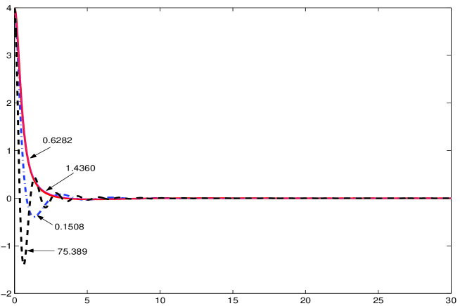
Figure 2: Real part of the integrand for a call option for different values of the moneyness. The plots related to our data ($0.6282$ and $1.4360$) are very similar.

The numerical implementation was developed in the MatLab^© environment. Quadrature algorithms are needed to evaluate the option prices from (18): adaptive Simpson and Gauss-Lobatto quadrature rules, as available in MatLab, performed equally well, for typical values of the parameters. As a matter of fact the integrands are not rapidly oscillating and decrease sufficiently fast (e.g. see Fig. (2)). The FFT algorithm was implemented following Lee (2004), i.e. by sampling $F$ at the midpoints of intervals of length $\Delta$, $u_{n}=(n-\frac{1}{2})\Delta$, $n=1,\ldots,N$ and taking $\gamma\Delta=2\pi/N$. We get

$$\Sigma_{N}(k_{m})=\frac{\Delta}{\pi}\Re\left[\sum_{n=1}^{N}\mathrm{e}^{-\mathrm{i}(n-\frac{1}{2})\Delta(k_{1}+\gamma(m-1))}F((n-\frac{1}{2})\Delta)\right]$$

$$=\frac{\Delta}{\pi}\Re\left[\mathrm{e}^{-\mathrm{i}\frac{\pi}{N}(m-1)}\sum_{n=1}^{N}\mathrm{e}^{-\mathrm{i}\frac{2\pi}{N}(n-1)(m-1)}f(n)\right]$$

where $f(n)=F((n-\frac{1}{2})\Delta)\mathrm{e}^{-\mathrm{i}(n-\frac{1}{2})\Delta k_{1}}$. In this case we used $\gamma=0.01$ and $\nu=0.5$.

For the calibration we minimized the sum of squared errors by using the constrained minimization routine in MatLab. In fact, for the regime switching models we have to add the constraint $\sigma_{1}>\sigma_{2}$. The results obtained are reported in Table (3): RMSE and relative errors $\frac{\hat{C}-C_{0}(s_{0},K)}{\hat{C}}$ were calculated in the four cases. In Table (4) we report out-of-sample performances of each fitted model: these were obtained by calculating the deviation from five call option prices having a much longer maturity, i.e. $631$ days and moneyness ranging from $0.7539$ to $1.0052$.

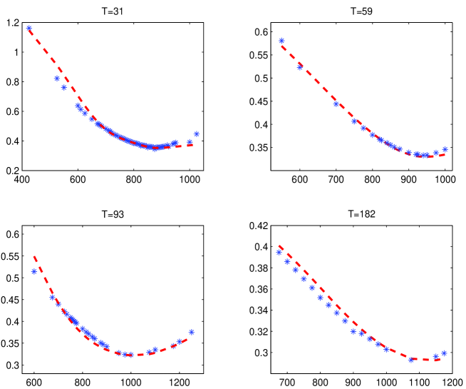
Figure 3: Implied volatility calibration.

	BS	RSBS	JDM	RSJDM
$\sigma_{1}$	0.3645	0.4462	0.1341	0.2725
$\sigma_{2}$		0.3296		0.1350
$\lambda_{1}$			7.9958	6.8393
$\lambda_{2}$				0.8590
$a_{1}$			-0.1280	-0.1398
$a_{2}$				-0.3423
$b_{1}$			0.0011	0.0877
$b_{2}$				0.1593
$q_{1}$		9.6199		6.5075
$q_{2}$		0.0002		0.0020
RMSE	4.6947	3.9177 ($i_{0}=1$)	3.8715	0.6126 ($i_{0}=1$)
Rel. err.	(-0.0242,0.1398) 0.0888	(-0.0141, 0.0631) 0.0353	(-0.0508, 0.1547) 0.0675	(-0.0080, 0.0191) 0.0041

Table 3: Implied parameters and in-sample calibration performances of the models. The moneyness of these options ranges from $0.6282$ to $1.4360$. In the last rows we report the range and the mean of the relative pricing error $\frac{\hat{C}-C_{M}}{\hat{C}}$.

	BS	RSBS	JDM	RSJDM
RMSE	14.8555	6.4732	17.1020	5.1116
Mean Rel Err.	-0.1852	-0.0631	-0.2142	-0.0634

Table 4: Out-of-sample performance of the models. The moneyness of these options ranges from $0.7539$ to $1.0052$.

4 On the pricing of forward starting options

Forward starting options are well-known exotic derivatives, depending on an underlying asset characterized by the payoff

$$\Pi_{T}(S(T),\kappa)=S(T)-\kappa S(t^{*}),$$ (22)

where $t^{*}\in(0,T)$ is the determination time and $\kappa\in(0,1)$ is a given percentage. They are the building blocks of the so-called cliquet options and are used in many different context.

In this Section we provide a simple valuation formula for the price at time $t=0$ of this claim where the underlying $S(t)$ follows the regime-switching jump diffusion dynamic introduced in Sect. 2. Furthermore, we assume that $\mu(\alpha)=r$, the risk-free rate, in such a way $\mathcal{P}\equiv\mathcal{Q}$. The risk-neutral price is therefore given by

$$\Pi_{0}(s_{0},\alpha_{0},\kappa)=\mathbf{E}[\mathrm{e}^{-rT}(S(T)-\kappa S(t^{*}))^{+}]=\mathbf{E}[\mathrm{e}^{-rT}(s_{0}\mathrm{e}^{X(T)}-\kappa S(t^{*}))^{+}].$$

Notice that in general from the determination time $t^{*}$ on, the price is equal to that of a standard call option, being the strike a known constant. By denoting with $\mathbf{E}_{t}[\cdot]$ the conditional expectation w.r.t. information up to time $t$, $\mathcal{F}_{t}$, we have

$$C_{t}(S(t),\alpha(t),K)=\mathbf{E}_{t}[\mathrm{e}^{-r(T-t)}(S(T)-K)^{+}]=\mathrm{e}^{-r(T-t)}\mathbf{E}_{t}[(S(t)\mathrm{e}^{X_{t,T}}-K)^{+}].$$

Therefore, if $K=\kappa S(t)$ we get that

$$C_{t}(S(t),\alpha(t),\kappa S(t))=S(t)C_{t}(1,\alpha(t),\kappa).$$

Hence, by the law of iterated conditional expectations,

$$\Pi_{0}(s_{0},\alpha_{0},\kappa)=\mathbf{E}[\mathrm{e}^{-rT}(S(t^{*})\mathrm{e}^{X_{t^{*},T}}-\kappa S(t^{*}))^{+}]=\mathbf{E}[\mathrm{e}^{-rt^{*}}C_{t^{*}}(S({t^{*}}),\alpha({t^{*}}),\kappa S({t^{*}}))]=$$

$$=\mathbf{E}[S(t^{*})\mathrm{e}^{-rt^{*}}C_{t^{*}}(1,\alpha(t^{*}),\kappa)].$$

Since $S(t)\mathrm{e}^{-rt}=S(t)/B(t)$ is a $\mathcal{Q}$-martingale we can introduce an equivalent measure $Q^{S}$ as

$$L(t)=\frac{dQ^{S}}{dQ}|_{t}=\frac{S(t)}{B(t)}\frac{B(0)}{s_{0}},\ \ \mathbf{E}[L(T)]=1,$$

from which we get

$$\mathbf{E}[S(t^{*})\mathrm{e}^{-rt^{*}}C_{t^{*}}(1,\alpha(t^{*}),\kappa)]=s_{0}\mathbf{E}^{Q^{S}}[C_{t^{*}}(1,\alpha(t^{*}),\kappa)].$$

Notice that this property is fairly general: in fact $\alpha(t)$ is not restricted to be a Markov chain. On the other hand, in our model we don’t need to further specify the $Q^{S}$ dynamic of the price process, since the Markov chain is not affected by this change of measure. Hence, since the chain is assumed to be stationary, by denoting with $\mathbf{\pi}=(\pi_{1},\ldots,\pi_{M})^{\prime}$ its invariant probability, we get

$$\Pi_{0}(s_{0},\kappa)=s_{0}\mathbf{E}^{Q^{S}}[C_{t^{*}}(1,\alpha(t^{*}),\kappa)]=s_{0}\sum_{j=1}^{M}\pi_{j}C_{t^{*}}(1,j,\kappa).$$

The price of the forward starting option is therefore the mixture of call option prices evaluated at the determination time $t^{*}$ under each regime weighted by the corresponding probability. By using transform representation for the call option value, e.g. (18), we get the following proposition.

Proposition 4.1

Let the underlying be characterized by the SDE (7). Then the price at time $t=0$ of the Forward Starting Option (22) with determination time $t^{*}$ and percentage $\kappa\in(0,1)$ is given by

$$\Pi_{0}(s_{0},\kappa)=s_{0}\mathrm{e}^{-r(T-t^{*})}\sum_{j=1}^{M}\pi_{j}\left(R_{\nu}+\frac{\kappa^{1-\nu}}{\pi}\int_{0}^{+\infty}\Re\left[\frac{\mathrm{e}^{-\mathrm{i}u\log(\kappa)}\mathrm{q}_{j}^{t^{*},T}(u-\mathrm{i}\nu)}{\nu^{2}-\nu-u^{2}-\mathrm{i}u(1-2\nu)}\right]du\right),$$

where $\{\pi_{j}\}_{j=1,\ldots,m}$ is the stationary probability of the Markov chain, $\nu$ and $R_{\nu}$ following from (18). $\Box$

As a byproduct of the last proposition, by restricting our model to a unique regime (see Remark (3.2)), we get a simple formula for pricing a FSO in a Lévy model with finite activity.

The impact of model choice on the prices of the Forward Starting options is shown in figures (4), (5) and (6) as a function of the determination time for three different values of the percentage $\kappa$. The parameters of each model are those estimated in our numerical example (Table (3)).

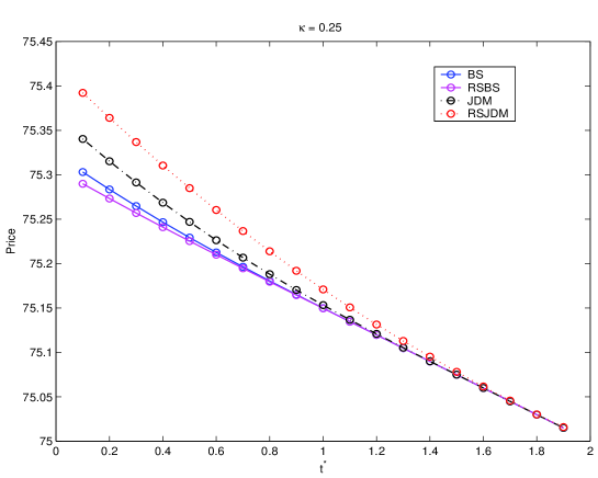
Figure 4: Forward starting option prices.

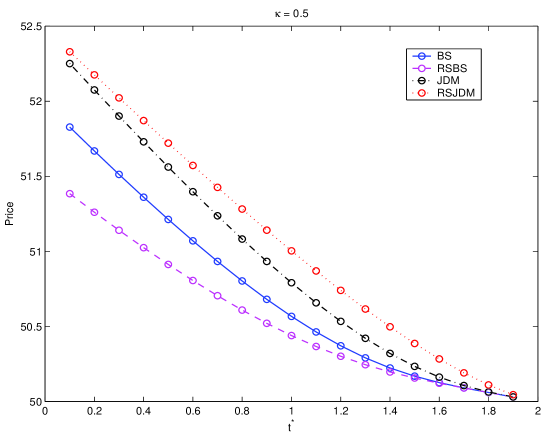
Figure 5: Forward starting option prices.

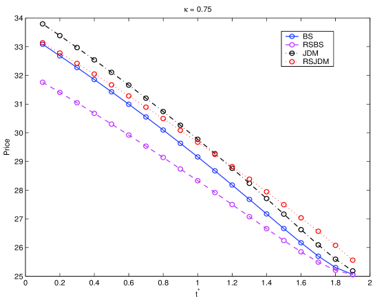
Figure 6: Forward starting option prices.

Pricing FSO in a general stochastic volatility model.

In Chourdakis (2004) a regime-switching diffusion was considered to approximate a general stochastic volatility model

$$dX(t) = \mu(v(t))dt+\sigma(v(t))dW(t)+\int_{\mathbb{R}}yp^{\alpha}(dy,dt),$$ (23)

$$dv(t) = a(v(t))dt+b(v(t))dZ(t),$$ (24)

where $X(t)=\log(S(t))$ and $p^{\alpha}(dy,dt)$ has intensity $\lambda(t,v,dy)=\lambda(v)m_{v}(y)dy$, $m_{v}$ being the probability measure which characterizes the jump component. Then, under some conditions on the coefficients $a(\cdot)$ and $b(\cdot)$, the diffusion process (24) can be approximated by a finite state Markov chain defined on a grid $G^{\epsilon}$ which is the discretization of the domain of $v$. The approximating scheme defines a generator $Q^{\epsilon}$ for the Markov chain depending on $\epsilon$ and on the functions $a(\cdot)$ and $b(\cdot)$ evaluated at the points of the grid $G^{\epsilon}=\{v^{\epsilon}_{1},\ldots,v^{\epsilon}_{M}\}$. As reported in Chourdakis (2004) the generator $Q^{\epsilon}=\{q^{\epsilon}_{ij}\}_{i,j=1,\ldots,M}$ where

$$q^{\epsilon}_{ij}=\left\{\begin{array}[]{ll}\frac{1}{2\epsilon^{2}}b^{2}(v^{\epsilon}_{j})-\frac{1}{2\epsilon}a(v^{\epsilon}_{j}),&i=j-1\\ \\ \frac{1}{\epsilon^{2}}b^{2}(v^{\epsilon}_{j}),&i=j\\ \\ \frac{1}{2\epsilon^{2}}b^{2}(v^{\epsilon}_{j})+\frac{1}{2\epsilon}a(v^{\epsilon}_{j}),&i=j+1\\ \\ 0&i\neq j-1,j,j+1\\ \end{array}\right.$$ (25)

produces accurate results for coarse volatility grids. The resulting approximated process $X^{\epsilon}(t)$ follows therefore a RSJD dynamic and its characteristic function is obtained from Prop. (3.1). Correspondingly, option prices can be calculated by means of the Fourier transform techniques presented in Sect. 3. Convergence properties as well as computational considerations as $\epsilon\rightarrow 0$ are discussed in Chourdakis (2004) where a number of cases are studied.

This technique combined with our Proposition (4.1) suggests the following scheme for pricing FSO under a general SV model:

1. approximate the model with a regime-switching diffusion $X^{\epsilon}(t)$: this amounts to build the generator $Q^{\epsilon}$ of the Markov chain, defined by (25);

2. evaluate call option prices $C^{\epsilon}_{j}$ at time $t^{*}$ under each regime $j=1,\ldots,M$ through formula (18) or (21) with $S(t^{*})=1$ and $K=\kappa$;

3. calculate the price $\Pi_{0}(s_{0},\kappa)=s_{0}\sum_{j=1}^{M}\pi_{j}C^{\epsilon}_{j}$ where the coefficients $\pi_{j}$’s are the solution of $\pi Q^{\epsilon}=0$.

5 Conclusion

In this paper we considered the problem of valuing the price of a European contingent claim when the underlying dynamic follows a Lèvy process of I type whose parameters are modulated by a continuous time and finite state Markov chain. These kind of processes are known to capture specific features of financial time series, such as volatility clustering and structural breaks. On the other hand, they can equally be used to approximate very general stochastic volatility processes. Following the well established relationship between option prices and Fourier transforms, we obtained almost closed-form solutions (up to a numerical integration) for European style options, both in log-price and in log-strike space. An example of calibration for the regime-switching version of the Merton jump-diffusion model is also presented for a daily set of call option data on the S&P 500.

Furthermore, as a practical application of the Fourier transform methodology we obtained an almost closed-form solution to the problem of valuing a Forward Starting option in our general regime-switching jump-diffusion dynamic. This result can be jointly used with the approximation scheme of stochastic volatility models to get a feasible algorithm for FSO pricing under a very general dynamic.

6 Appendix

Proof of 2.1

Let us define the occupation times for the Markov chain $\alpha(t)$ in $[0,T]$, $T_{i}=\int_{0}^{T}\mathbb{I}_{\alpha(s)=i}ds$, $i=1,\ldots,M$. We immediately have that $\sum_{i=1}^{m}T_{i}=T$. Now, given a sample path of the chain $\alpha(t),0\leq t\leq T$, we can define

$$\Delta_{i} = \bigcup_{\ell:\ \alpha(t)=i,\tau_{\ell}\leq t<\tau_{\ell+1}}[\tau_{\ell},\tau_{\ell+1})$$ (26)

$$N(\Delta_{i}) = \sum_{\ell:\ \alpha(t)=i,\tau_{\ell}\leq t<\tau_{\ell+1}}\left(N_{\tau_{\ell+1}}-N_{\tau_{\ell}}\right)$$ (27)

$$Z(\Delta_{i}) = \sum_{\ell:\ \alpha(t)=i,\tau_{\ell}\leq t<\tau_{\ell+1}}\left(W(\tau_{\ell+1})-W(\tau_{\ell})\right).$$ (28)

Since each $\Delta_{i}$ is the union of non overlapping intervals, the corresponding random variables $N(\Delta_{i})$ and $Z(\Delta_{i})$ are distributed as a Poisson variable $\mathrm{Poiss}(\lambda_{i}T_{i})$ and as a Normal variable $\mathcal{N}(0,T_{i})$, respectively. Furthermore, $N(\Delta_{i})\perp N(\Delta_{j})$ and $Z(\Delta_{i})\perp Z(\Delta_{i})$, for $i\neq j$. By denoting with $Y^{(i)}_{k}$ the $k$-th jump magnitude relative to regime $i$, we have

$$J(t)=\sum_{i=1}^{M}\sum_{k=1}^{N(\Delta_{i})}Y^{(i)}_{k}\ \ \ \mbox{and}\ \ \int_{0}^{T}\sigma(\alpha(s))dW(s)=\sum_{i=1}^{m}\sigma(i)Z(\Delta_{i})\sim\mathcal{N}(0,\sum_{i=1}^{m}\sigma_{i}^{2}T_{i})$$ (29)

By defining $\xi(\alpha)=\mu(\alpha)-\frac{1}{2}\sigma^{2}(\alpha)-\lambda(\alpha)\kappa(\alpha)$ and

$$\Xi_{T}(T_{1},\ldots,T_{m})=\int_{0}^{T}\xi(\alpha(s))ds=\sum_{i=1}^{m}\xi(i)T_{i}$$

then $X(T)$ admits the following representation:

$$X(T)=\Xi_{T}(T_{1},\ldots,T_{m})+\sum_{i=1}^{m}\sigma(i)Z(\Delta_{i})+\sum_{i=1}^{M}\sum_{k=1}^{N(\Delta_{i})}Y^{(i)}_{k}.$$ (30)

Proof of 3.1

Let $\phi_{j}(z)=\mathbf{E}[\mathrm{e}^{\mathrm{i}z\gamma(Y(j),j)}]$ be the generalized Fourier transform of the jump magnitude. From the representation (30) we can easily calculate the characteristic function of $X(T)$, conditional to $\mathcal{F}^{\alpha}_{T}$:

$$\mathbf{E}[\mathrm{e}^{\mathrm{i}zX(T)}|\mathcal{F}^{\alpha}_{T}]=\mathrm{e}^{\mathrm{i}z\Xi_{T}(T_{1},\ldots,T_{m})}\ \mathbf{E}[\mathrm{e}^{\mathrm{i}z\sum_{j=1}^{m}\sigma(j)Z(\Delta_{j})}|\mathcal{F}^{\alpha}_{T}]\ \mathbf{E}[\mathrm{e}^{\mathrm{i}z\sum_{j=1}^{M}\sum_{k=1}^{N(\Delta_{j})}\gamma(Y^{(j)}_{k},j)}|\mathcal{F}^{\alpha}_{T}].$$

The first expected value is simply obtained as

$$\mathbf{E}[\mathrm{e}^{\mathrm{i}z\sum_{j=1}^{m}\sigma(i)Z(\Delta_{j})}|\mathcal{F}^{\alpha}_{T}]=\mathrm{e}^{-\frac{1}{2}z^{2}\sum_{j=1}^{m}\sigma_{j}^{2}T_{j}},$$

while the second, since $N(\Delta_{i})\perp N(\Delta_{j})$ for $i\neq j$, is

$$\mathbf{E}[\mathrm{e}^{\mathrm{i}z\sum_{j=1}^{M}\sum_{k=1}^{N(\Delta_{j})}\gamma(Y^{(j)}_{k},j)}|\mathcal{F}^{\alpha}_{T}]=\mathrm{e}^{\sum_{j=1}^{m}\lambda_{j}T_{j}(\phi_{j}(z)-1)}.$$

Finally, we have

$$\varphi_{T}(z)=\mathbf{E}\left[\mathrm{e}^{\mathrm{i}z\Xi_{T}(T_{1},\ldots,T_{m})-\frac{1}{2}z^{2}\sum_{j=1}^{m}\sigma_{j}^{2}T_{j}+\sum_{j=1}^{m}\lambda_{j}T_{j}(\phi_{j}(z)-1)}\right].$$ (31)

Actually, the exponent in (31) is a linear function of the sojourn times $T_{1},\ldots,T_{m}$, the characteristic function of which are well-known. As a matter of fact, we have

$$\varphi_{T}(z)=\mathbf{E}\left[\mathrm{e}^{\mathrm{i}\sum_{j=1}^{m}\vartheta_{j}(z)T_{j}}\right]=\mathrm{e}^{\mathrm{i}\vartheta_{m}(z)T}\mathbf{E}\left[\mathrm{e}^{\mathrm{i}\sum_{j=1}^{m-1}\tilde{\vartheta}_{j}(z)T_{j}}\right]$$ (32)

where $\tilde{\vartheta}_{i}(z)=\vartheta_{i}(z)-\vartheta_{m}(z)$, being $T_{m}=T-(T_{1}+\ldots+T_{m-1})$. Since it can be proved (see e.g. Buffington and Elliott (2002)), that

$$\mathbf{E}\left[\mathrm{e}^{\mathrm{i}\sum_{j=1}^{m-1}\tilde{\vartheta}_{j}T_{j}}\right]=\mathbf{1}^{\prime}\cdot\mathrm{e}^{Q^{\prime}+\mathrm{i}\mathrm{diag}(\tilde{\vartheta}_{1},\ldots,\tilde{\vartheta}_{m-1},0)T}\cdot\mathbb{I}(0),$$

formula (12) follows, the second equality being a consequence of the property of matrix exponential $\exp(\theta)\exp(A)=\exp(\theta I+A)$.

Derivation of Tables 2.

Payoff $\mathrm{e}^{ax}\mathbb{I}_{bx>\kappa}$. From the third row of Table 1 and formula (10) we get for log-price transform

$$\Pi_{0}/P(0,T)=\frac{1}{2\pi}\int_{\mathrm{i}\nu-\infty}^{\mathrm{i}\nu+\infty}\mathrm{e}^{-\mathrm{i}z\log(s_{0})}\frac{\mathrm{e}^{(a+\mathrm{i}z)k/b}}{a+\mathrm{i}z}\varphi_{T}(-z)dz=$$

$$\frac{1}{2\pi}s_{0}^{\nu}\mathrm{e}^{(a-\nu)k/b}\int_{-\infty}^{+\infty}\frac{\mathrm{e}^{-\mathrm{i}u(\log(s_{0})-k/b)}\varphi_{T}(-u-\mathrm{i}\nu)}{\nu-a-\mathrm{i}u}du=$$

$$\frac{1}{\pi}s_{0}^{\nu}\mathrm{e}^{(a-\nu)k/b}\int_{0}^{+\infty}\Re\left[\frac{\mathrm{e}^{-\mathrm{i}u(\log(s_{0})-k/b)}\varphi_{T}(-u-\mathrm{i}\nu)}{\nu-a-\mathrm{i}u}\right]du,\ \ \ \nu>a;$$

for log-strike transform

$$\mathbf{E}[\hat{\Pi}_{X(T)+\log(s_{0})}(k)]=\mathbf{E}[\frac{\mathrm{e}^{(a+\mathrm{i}zb)(\log(s_{0})+X(T))}}{\mathrm{i}z}]=\frac{\mathrm{e}^{(a+\mathrm{i}zb)\log(s_{0})}}{\mathrm{i}z}\varphi_{T}(a+\mathrm{i}zb)$$

from which

$$\Pi_{0}/P(0,T)=\frac{1}{2\pi}\int_{\mathrm{i}\nu-\infty}^{\mathrm{i}\nu+\infty}\mathrm{e}^{-\mathrm{i}zk}\frac{\mathrm{e}^{(a+\mathrm{i}zk)\log(s_{0})}}{\mathrm{i}z}\varphi_{T}(a+\mathrm{i}bz)dz=$$

$$\frac{1}{2\pi}s_{0}^{a-b\nu}\mathrm{e}^{\nu k}\int_{-\infty}^{+\infty}\frac{\mathrm{e}^{-\mathrm{i}u(k-b\log(s_{0}))}}{\mathrm{i}u-\nu}\varphi_{T}(a-\nu b+\mathrm{i}bu)du=$$

$$\frac{1}{\pi}s_{0}^{a-b\nu}\mathrm{e}^{\nu k}\int_{0}^{+\infty}\Re\left[\frac{\mathrm{e}^{-\mathrm{i}u(k-b\log(s_{0}))}}{\mathrm{i}u-\nu}\varphi_{T}(a-\nu b+\mathrm{i}bu)\right]du,\ \ \ \nu>0.$$

Payoff $\min(\mathrm{e}^{x},\mathrm{e}^{k})$. From the fourth row of Table 1 and formula (10) we get for log-price transform

$$\Pi_{0}/P(0,T)=\frac{1}{2\pi}\int_{\mathrm{i}\nu-\infty}^{\mathrm{i}\nu+\infty}\mathrm{e}^{-\mathrm{i}z\log(s_{0})}\frac{\mathrm{e}^{k(\mathrm{i}z+1)}}{z^{2}-\mathrm{i}z}\varphi_{T}(-z)dz=$$

$$\frac{1}{2\pi}s_{0}^{\nu}\mathrm{e}^{k(1-\nu)}\int_{-\infty}^{+\infty}\frac{\mathrm{e}^{-\mathrm{i}u(\log(s_{0})-k)}}{u^{2}-\nu^{2}+\nu+\mathrm{i}u(2\nu-1)}\varphi_{T}(-u-\mathrm{i}\nu)du=$$

$$\frac{1}{\pi}s_{0}^{\nu}\mathrm{e}^{k(1-\nu)}\int_{-\infty}^{+\infty}\Re\left[\frac{\mathrm{e}^{-\mathrm{i}u(\log(s_{0})-k)}}{u^{2}-\nu^{2}+\nu+\mathrm{i}u(2\nu-1)}\varphi_{T}(-u-\mathrm{i}\nu)\right]du,\ \ \ 0<\nu<1;$$

for log-strike transform

$$\mathbf{E}[\hat{\Pi}_{X(T)+\log(s_{0})}(k)]=\mathbf{E}[\frac{\mathrm{e}^{(1+\mathrm{i}z)(\log(s_{0})+X(T))}}{z^{2}-\mathrm{i}z}]=\frac{\mathrm{e}^{(1+\mathrm{i}z)\log(s_{0})}}{z^{2}-\mathrm{i}z}\varphi_{T}(z-\mathrm{i})$$

from which

$$\Pi_{0}/P(0,T)=\frac{1}{2\pi}\int_{\mathrm{i}\nu-\infty}^{\mathrm{i}\nu+\infty}\mathrm{e}^{-\mathrm{i}zk}\mathrm{e}^{-\mathrm{i}zk}\frac{\mathrm{e}^{(1+\mathrm{i}z)\log(s_{0})}}{z^{2}-\mathrm{i}z}\varphi_{T}(z-\mathrm{i})dz=$$

$$\frac{1}{2\pi}\mathrm{e}^{\nu k}s_{0}^{1-\nu}\int_{-\infty}^{+\infty}\frac{\mathrm{e}^{-\mathrm{i}u(k-\log(s_{0}))}}{u^{2}-\nu^{2}+\nu+\mathrm{i}u(2\nu-1)}\varphi_{T}(u+\mathrm{i}(\nu-1))du=$$

$$\frac{1}{\pi}\mathrm{e}^{\nu k}s_{0}^{1-\nu}\int_{0}^{+\infty}\Re\left[\frac{\mathrm{e}^{-\mathrm{i}u(k-\log(s_{0}))}}{u^{2}-\nu^{2}+\nu+\mathrm{i}u(2\nu-1)}\varphi_{T}(u+\mathrm{i}(\nu-1))\right]du,\ \ \ 0<\nu<1.$$

By substituting in the previous formulas the GFT (13) of the RSJD model, we immediately get the entries of Table 2.

References

Bakshi G. and Madan D. (2000), Spanning and derivative-securities valuation, Journal of Financial Economics, 55, pp. 205-238.

F. Biagini, Y. Bregman, and T.Meyer-Brandis, Pricing of catastrophe insurance options written on a loss index with reestimation, Insurance Math. Econom., 43 (2008), pp. 214-222.

Bollen N. P. B. (1998), Valuing options in regime-switching models. Journal of Derivatives, 6, pp. 38-49.

K. Borovkov and A. Novikov, On a new approach to calculating expectations for option pricing, J. Appl. Probab., 39 (2002), pp. 889-895.

Boyarchenko S., Levendorskii S., American options in regime-switching models. SIAM J. Control Optim. 48 (2009), no. 3, pp. 1353-1376.

Boyle P. and Draviam T. (2007), Pricing exotic options under regime switching, Insurance: Mathematics and Economics, 40 , pp. 267-282.

Buffington J. and Elliott R. J. (2002), American options with regime switching, International Journal of Theoretical and Applied Finance, 5 , pp. 497-514.

Carr P. and Madan D.B. (1999), Option valuation using the Fast Fourier Transform, Journal of Computational Finance, 2, pp. 61-73.

Cherubini U., Della Lunga G., Mulinacci S., Rossi P., Fourier Transform Methods in Finance, Wiley, 2009.

Chourdakis K. (2004), Non-Affine option pricing, The Journal of derivatives, 2004, pp. 10-25.

Chourdakis K. (2007), Lévy process driven by stochastic volatility, Asia-Pacific Financial Markets, Vol. 12, No. 4, pp. 333-352.

Cont R. and Tankov P. (2004), Financial Modelling with Jump Processes, Chapman & Hall/CRC Financial Mathematics Series.

Di Graziano G. and Rogers L. C. G. (2009), Equity with Markov-modulated dividends, Quantitative Finance, Vol. 9, No. 1, pp. 19-26.

Di Masi, G.B., Kabanov, Y.M., Runggaldier,W.J. (1994), Mean-variance hedging of options on stocks with Markov volatility, Theory of Probability and Its Applications, 39, pp. 173-181.

Duan, J.C., Popova, I., Ritchken, P. (2002), Option pricing under regime switching, Quantitative Finance, 2, pp. 1-17.

D. Dufresne, J. Garrido, and M. Morales, Fourier inversion formulas in option pricing and insurance, Methodol. Comput. Appl. Probab., 11 (2009), pp. 359-383.

E. Eberlein, K. Glau, and A. Papapantoleon, Analysis of Fourier transform valuation formulas and applications, Appl. Math. Finance, 17 (2010), pp. 211-240.

Edwards C. (2005), Derivative Pricing Models with Regime Switching. A General Approach, The Journal of Derivatives, Vol. 13, No. 1, pp. 41-47.

Elliott R. J. and Osakwe C. J. U. (2006), Option pricing for pure jump processes with Markov switching compensators, Finance and Stochastics, 10, pp. 250-275.

Elliott R. J. , Siu T. K. and Chan L. (2007), Pricing volatility swaps under Heston’s stochastic volatility model with regime switching, Applied Mathematical Finance, Vol 14, 1, pp. 41-62.

Guo X., (2001), Information and option pricing Quantitative Finance, 1, pp. 38-44.

Guo X. and Zhang Q. Z (2004), Closed-form solutions for perpetual American put options with regime switching, SIAM Journal of Applied Mathematics, 64 , pp. 2034-2049.

Hamilton, J.D., (1989), A new approach to the economic analysis of non-stationary time series, Econometrica, 57, pp. 357-384.

Hamilton, J.D., (1990), Analysis of time series subject to changes in regime, Journal of Econometrics, 45, pp. 39-70.

Hardy, M.R., (2001), A regime switching model of a long term stock-returns. North American Actuarial Journal, 3, pp. 185-211.

Heston, S. L. A. (1993), Closed-Form Solution for Options with Stochastic Volatility with Applications to Bond and Currency Options, Rev. Fin. Studies, vol. 6, 327-343.

Higham N. J., (2009), The scaling and Squaring Method for the Matrix Exponential Revisited, SIAM Review, Vol. 51, No. 4, pp. 747-764.

F. Hubalek, J. Kallsen, and L. Krawczyk, Variance-optimal hedging for processes with stationary independent increments, Ann. Appl. Probab., 16 (2006), pp. 853-885.

T. R. Hurd and Z. Zhou, A Fourier transform method for spread option pricing, SIAM J. Financial Math., 1 (2010), pp. 142-157.

Jiang Z., Pistorius M. R. On perpetual American put valuation and first-passage in a regime-switching model with jumps. Finance Stoch. 12 (2008), no. 3, 331-355.

Jobert A. and Rogers L. C. G. (2006), Option pricing with Markov-Modulated dynamics, SIAM Journal of Control and Optimization, Vol. 44, No. 6, pp. 2063-2078.

Khaliq, A. Q. M.; Liu, R. H. New numerical scheme for pricing American option with regime-switching. Int. J. Theor. Appl. Finance 12 (2009), no. 3, 319-340.

Konikov M. and Madan D. B. (2002), Option Pricing Using Variance Gamma Markov Chains, Review of Derivatives Research, Vol. 5, No. 1, pp. 81-115

Kruse S. and Nögel U. (2005), On the pricing of forward starting options in Heston’s model on stochastic volatility, Finance and Stochastics, 9, pp. 233-250.

Lee R. W. (2004), Option pricing by transform methods: extensions, unifications and error control, Journal of Computational Finance, 7, pp. 51-86.

Lewis A.L. (2002), A simple option formula for general jump-diffusion and other exponential Lévy processes, Working Paper, Optioncitynet.net.

Liu, R. H. Regime-switching recombining tree for option pricing. Int. J. Theor. Appl. Finance 13 (2010), no. 3, 479-499.

Liu R. H. , Zhang Q. , and Yin G. (2006), Option pricing in a regime-switching model using the fast Fourier transform. J. Appl. Math. Stoch. Anal., Vol. 22, pp.1-22.

R. Lord (2008), Efficient pricing algorithms for exotic derivatives, PhD thesis, Univ. Rotterdam.

Naik, V. (1993), Option valuation and hedging strategies with jumps in the volatility of asset returns. Journal of Finance, 48, pp. 1969-1984.

S. Raible (2000), L evy processes in finance: Theory, numerics, and empirical facts., PhD thesis, Univ. Freiburg.

Ramponi A. (2009), Mixture Dynamics and Regime Switching Diffusions with Application to Option Pricing. Methodol. Comput. Appl. Probab., DOI 10.1007/s11009-009-9155-1

Runggaldier W.J. (2003) . Jump-Diffusion models, in ”Handbook of Heavy Tailed Distributions in Finance” (S.T. Rachev, ed.), Handbooks in Finance, Book 1 (W.Ziemba Series Ed.), Elesevier/North-Holland 2003, pp. 169-209.

Timmermann A. (2000), Moments of Markov switching models, Journal of Econometrics, 96, pp. 75-111.

Yao D. D., Zhang Q. and Zhou X. Y. (2006), A regime-switching model for European options, Stochastic Processes, Optimization, and Control Theory Applications in Financial Engineering, Queueing Networks, and Manufacturing Systems (H. M. Yan, G. Yin, and Q. Zhang, eds.), Springer, New York, pp. 281-300.